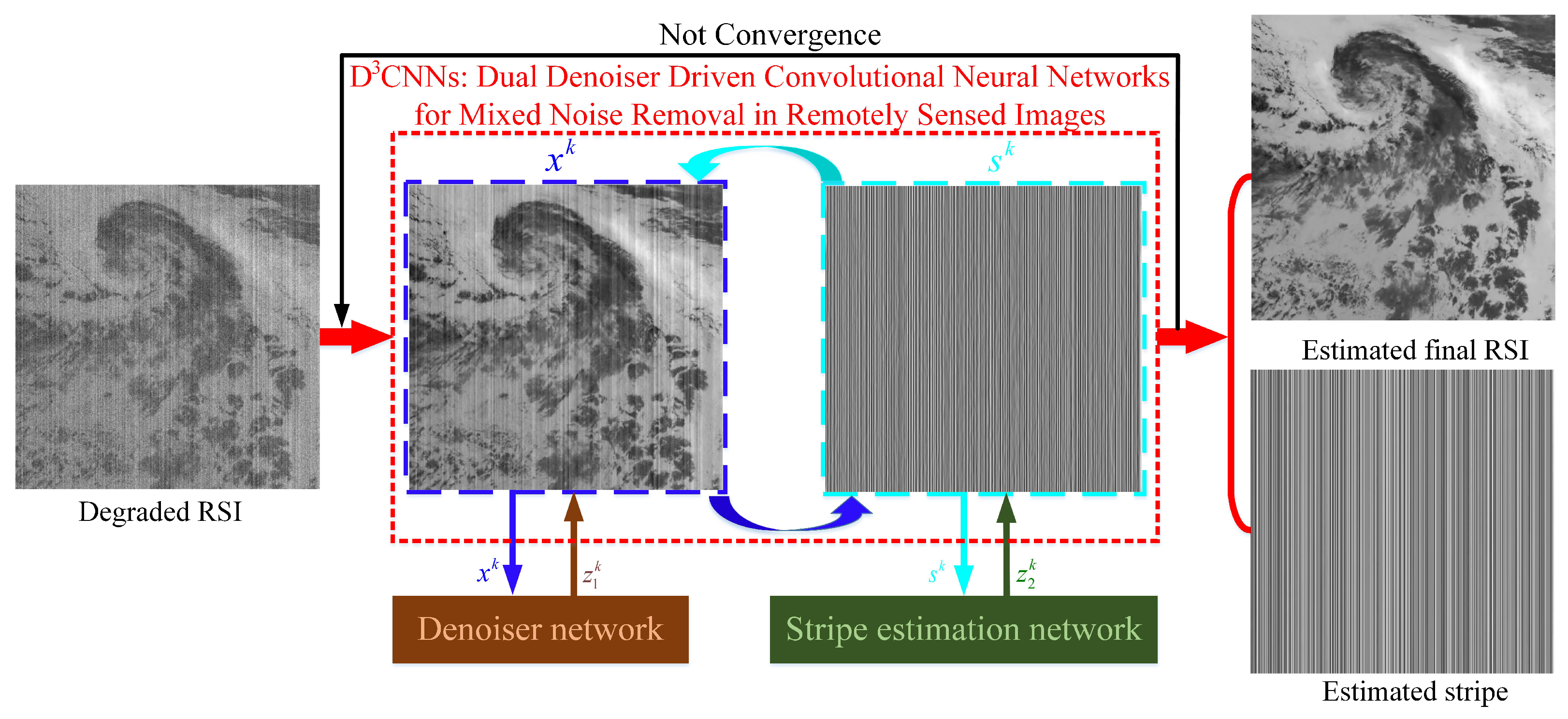
D³CNNs: Dual Denoiser Driven Convolutional Neural Networks for Mixed Noise Removal in Remotely Sensed Images

Abstract

Mixed (random and stripe) noise will cause serious degradation of optical remotely sensed image quality, making it hard to analyze their contents. In order to remove such noise, various inverse problems are usually constructed with different priors, which can be solved by either model-based optimization methods or discriminative learning methods. However, they have their own drawbacks, such as the former methods are flexible but are time-consuming for the pursuit of good performance; while the later methods are fast but are limited for extensive applications due to their specialized tasks. To fast obtain pleasing results with combination of their merits, in this paper, we propose a novel denoising strategy, namely, Dual Denoiser Driven Convolutional Neural Networks (D³CNNs), to remove both random and stripe noise. The D³CNNs includes the following two key parts: one is that two auxiliary variables respective for the denoised image and the stripe noise are introduced to reformulate the inverse problem as a constrained optimization problem, which can be iteratively solved by employing the alternating direction method of multipliers (ADMM). The other is that the U-shape network is used for the denoised auxiliary variable while the residual CNN (RCNN) for the stripe auxiliary variable. The subjectively and objectively comparable results of experiments on both synthetic and real-world remotely sensed images verify that the proposed method is effective and is even better than the state-of-the-arts.

1. Introduction

Remotely sensed images (RSIs) are “photographs” of the Earth’s surface, which can truly and vividly reflect the current situation of the distribution, the relationship, and the changes in the interaction of surface features, from which rich information including vegetation, soil moisture, water quality parameters, and surface and sea temperature can be obtained [1]. This Earth resource information can play an important role in the fields of agriculture, forestry [2], water conservancy, oceans, and ecological environment [3], which is beneficial for us to remotely investigate resources [4], monitor the environment [5], and analyze and predict disasters [6]. However, due to the impact of detector and photon effects, the obtained remotely sensed images may be degraded by both stripe noise (caused by the different responses of each detector) and random noise (which is mainly additive Gaussian white noise (AGWN) produced by photon effects) [7], which can be formulated as

$$y=x+s+n,$$

(1)

where y is the observed image, x is the latent clean image, s is the stripe noise, and n is the AGWN. It is an impossible task to simultaneously obtain s and x using Equation (1). To solve the problem, the common idea is the usage of a two-step method, such as first denoising [8,9,10,11,12,13,14,15,16,17,18,19,20,21,22,23,24,25,26,27,28,29,30,31,32,33,34,35,36,37,38] then destriping [39,40,41,42,43,44,45,46,47,48,49,50,51,52,53,54,55]. Such strategy may smooth many useful structures of image x. An example is shown in Figure 1, from which we can observe that many rich structures are smoothed. It is absolutely independent to reduce the two typical noise using the two-step method that may impair the structures of stripe or images and further smooth rich details. Therefore, one typical noise should be considered when the other is processed. To address this issue and preserve as many fine structures as possible, different regularizations on x and s are both considered to build a unified restoration model [56], which can be solved by the optimization methods (such as alternating direction method of multipliers (ADMM) and split Bregman). The procedures of these methods can be briefly presented as follows:

• According to the Bayes’ theorem, the estimation of x and s with the posterior distribution $P\left(x,s|y\right)$ can be converted into the following equation

  $$P\left(x,s|y\right)\propto P\left(y|x,s\right)P\left(x\right)P\left(s\right),$$

  (2)

  where $P\left(y|x,s\right)$ is a likelihood prior which can be presented as

  $$P\left(y|x,s\right)\propto exp\left\{-\frac{1}{2}{∥y-x-s∥}_2^2\right\},$$

  (3)

  where ${∥·∥}_2^2$ is the $l_2$-norm function. $P\left(x\right)$ and $P\left(s\right)$ are respectively the prior probabilities of x and s, which are used to obtain optimization solutions being closed to the actual values. With proper parameters ${\lambda }_1$ and ${\lambda }_2$, the prior probability $P\left(x\right)$ is written as

  $$P\left(x\right)\propto exp\left\{-{\lambda }_1\mathsf{\Phi }\left(x\right)\right\},$$

  (4)

  while $P\left(s\right)$ is defined as

  $$P\left(s\right)\propto exp\left\{-{\lambda }_2\mathsf{\Psi }\left(s\right)\right\},$$

  (5)

  where $\mathsf{\Phi }\left(·\right)$ and $\mathsf{\Psi }\left(·\right)$ are different regularizations on x and s, respectively. By inserting Equations (3) to (5) into Equation (2), the posterior distribution $P\left(x,s|y\right)$ is equivalent to

  $$P\left(x,s|y\right)\propto P\left(y|x,s\right)P\left(x\right)P\left(s\right)\propto exp\left\{-\left(\frac{1}{2}{∥y-x-s∥}_2^2+{\lambda }_1\mathsf{\Phi }\left(x\right)+{\lambda }_2\mathsf{\Psi }\left(s\right)\right)\right\}.$$

  (6)
• With the usage of the logarithmic transformation, the optimization solution of Equation (6) is transferred from maximizing the posterior distribution to minimizing the energy function $\mathcal{L}\left(x,s\right)=-log\left\{P\left(x,s|y\right)\right\}$ which is

  $$\mathcal{L}\left(x,s\right)=\frac{1}{2}{∥y-x-s∥}_2^2+{\lambda }_1\mathsf{\Phi }\left(x\right)+{\lambda }_2\mathsf{\Psi }\left(s\right).$$

  (7)
• The optimization solution of model (7) is solved with the employment of ADMM or split Bregman by introducing auxiliary variables.

2. Related Works

The stripe noise coexisting with the random noise makes it difficult to formulate the mixed noise with an explicit expression due to the nonindependent as well as nonidentical property. Usually, a unified energy model $\mathcal{L}$ is constructed by different penalty priors $\mathsf{\Phi }$ and $\mathsf{\Psi }$ respectively on image x and stripe s to separate them from image decomposition perspective [43], in which the stripe is equal to the image. According to the categories of priors, they are divided into the following three categories:

• Sparsity-based priors: These methods viewed that the image especially the stripe is sparse, so different priors, such as gradient-based variation, dictionary-based learning, and low-rank recovery, are combined to constrain the models for pursuing the optimal approximate solution. For instance, Huang et al. [56] proposed a uniform mixed noise removal model by the employment of joint analysis and weighted synthesis sparsity priors (JAWS). Chang et al. [57] employed unidirectional total variation and sparse representation (UTVSR) to simultaneously destripe and denoise remote sensing images. Xiong et al. [58] proposed a spectral-spatial $L_0$ gradient regularized low-rank tensor factorization method for hyperspectral denoising. Zheng et al. [59] removed mixed noise in hyperspectral images via low-fibered-rank regularization. Liu et al. [60] used the global and local sparsity constraints for a unified model construction to simultaneously estimation intensity bias and remove stripe noise in noisy infrared images. Zeng et al. [61] proposed a hyperspectral image restoration model with global L${}_{1–2}$ spatial-spectral total variation regularized local low-rank tensor recovery. Xie et al. [62] denoised hyperspectral images via non-convex regularized low-rank and sparse matrix decomposition. Hu et al. [63] proposed a restoration method that can simultaneously remove Gaussian noise and stripes using adaptive anisotropy total variation and nuclear norms. Wang et al. [64] presented a $l_0-l_1$ Hybrid total variation model for hyperspectral image mixed noise removal and compressed sensing. Wang et al. [65] exploited nonconvex logarithmic penalty for hyperspectral image denoising. These methods pursued their exciting denoising performance at the cost of expensively computational complexity.
• Sparsity-based priors with joint of deep CNN denoiser prior: Recently, deep convolutional neural network (CNN) as a prior for a specialized task has been popular applied in various fileds, especially in image restoration, due to its fast speed and large modeling capacity. Such property had been induced as an image prior to solve the inverse problem of image restoration [66,67,68], and had a considerable advantage. Inspired by its encouraging performance, Huang et al. [69] exploited deep CNN prior with the combination of unidirectional variation prior (UV-DCNN) to simultaneously destriping and denoising optical remotely sensed images. Zeng et al. [70] used CNN denoiser prior regularized low-rank tensor recovery for hyperspectral image restoration. These unfolding image denoising methods interpreted a truncated unfolding optimization as an end-to-end trainable deep network and thus usually produced pleasing results with fewer iterations using additional training for each task [68].
• Discriminative learning prior: As the Gaussian white noise and the stripe noise are both additive, so there are also various CNN-based denoising methods proposed to obtain both the image and the stripe. For example, He et al. [71] proposed a deep-learning approach to correct single-image-based nonuniformity in uncooled long-wave infrared detectors. Chang et al. [72] introduced a deep convolutional neural network (DCNN), named as HSI-DeNet, for HSIs’ noise removal. Zhang et al. [73] employed a spatial-spectral gradient network to remove hybrid noise in hyperspectral image. Luo et al. [74] suggested a spatial–spectral constrained deep image prior (S2DIP), which simultaneously capitalize the high model representation ability brought by the CNN in an unsupervised manner and does not need any extra training data. Despite the effectiveness of these methods, the CNN models are pretrained and cannot be jointly optimized with other parameters.

Inspired by the ideas in Refs. [66,67,68,69], in this paper, we proposed a unified mixed noise removal framework, named as Dual Denoiser Driven Convolutional Neural Networks (D³CNNs), to take advantages of both the optimization- and discriminative-learning-based methods. The flowchart of the proposed D³CNNs approach is shown in Figure 2. The main contributions of this paper are as follows:

• A unified mixed noise removal (MNR) framework, named as Dual Denoiser Driven Convolutional Neural Networks (D³CNNs), is proposed by using the CNN based denoiser and striper priors.
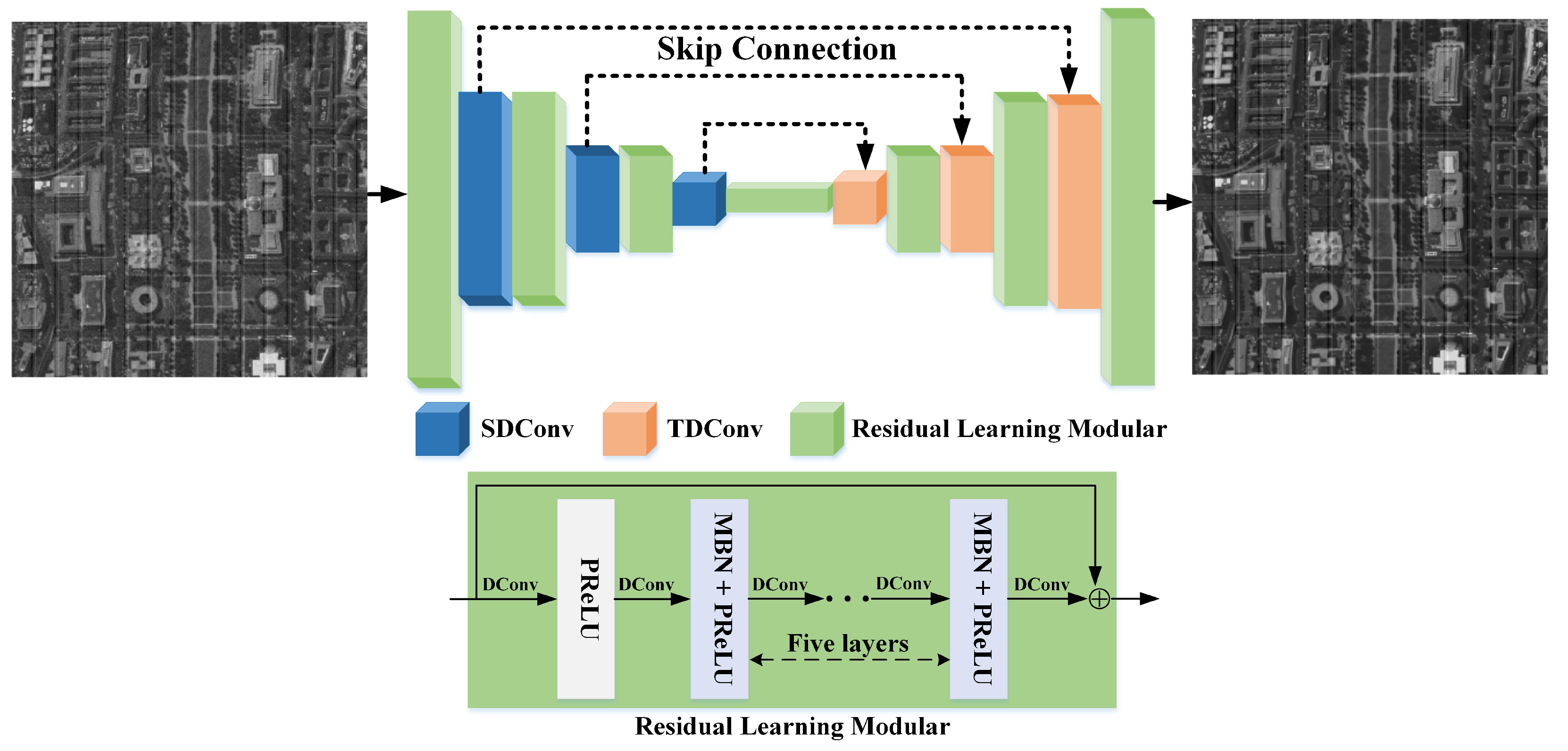
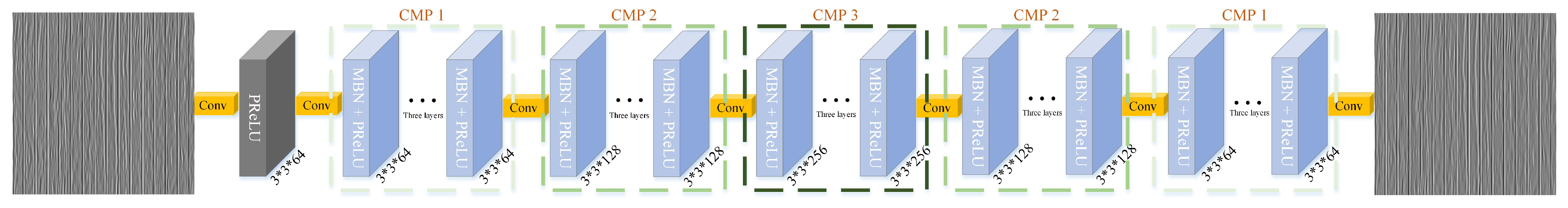
• Two deep denoiser/striper priors, respectively trained by a highly flexible U-shape denoiser and an effective residual learning strategy, are plugged as two modular parts into a half quadratic splitting based iterative algorithm to solve the inverse problem.
• Quantitative and qualitative results of experiments on both synthetic and real-world images validate the effectiveness of the proposed mixed noise removal scheme and even outperforms other advanced denoising approaches.

3. Dual Denoiser Driven Convolutional Neural Networks

Although various variable splitting algorithms can be employed to solve model (7), in this paper, we adopt half quadratic splitting (HQS) method due to its simplicity and fast convergence [68].

3.1. Half Quadratic Splitting (HQS) Algorithm

In order to plug the denoiser prior as well as the striper prior into the optimization procedure of Equation (7), two auxiliary variables $z_1$ and $z_2$ are introduced in HQS to decouple the data term and prior terms of Equation (7) and to reformulate it as a constrained optimization problem given by

$$\mathcal{L}\left(x,s\right)=\frac{1}{2}{∥y-x-s∥}^2+{\lambda }_1\mathsf{\Phi }\left(z_1\right)+{\lambda }_2\mathsf{\Psi }\left(z_2\right),s.t.z_1=x,z_2=s.$$

(8)

Then, Equation (8) is solved by minimizing the following cost function

$${\mathcal{L}}_{{\mu }_1,{\mu }_2}\left(x,s\right)=\frac{1}{2}{∥y-x-s∥}^2+{\lambda }_1\mathsf{\Phi }\left(z_1\right)+\frac{{\mu }_1}{2}{∥x-z_1∥}^2+{\lambda }_2\mathsf{\Psi }\left(z_2\right)+\frac{{\mu }_2}{2}{∥s-z_2∥}^2,$$

(9)

where ${\mu }_1$ and ${\mu }_2$ are penalty parameters that vary iteratively in a non-descending order. The problem (9) can be addressed by the usage of the alternating direction method of multipliers (ADMM), which iteratively solves the following subproblems for each variable while keeping the rest variables fixed:

$$\underset{x,s}{min}\frac{1}{2}{∥y-x-s∥}^2+\frac{{\mu }_1}{2}{∥z_1-x∥}^2+\frac{{\mu }_2}{2}{∥z_2-s∥}^2,$$

(10)

$$\underset{z_1}{min}{\lambda }_1\mathsf{\Phi }\left(z_1\right)+\frac{{\mu }_1}{2}{∥z_1-x∥}^2,$$

(11)

$$\underset{z_2}{min}{\lambda }_2\mathsf{\Psi }\left(z_2\right)+\frac{{\mu }_2}{2}{∥z_2-s∥}^2.$$

(12)

The subproblem (10) can be further separated into two subproblems, and then Equation (9) can be iteratively solved by the following subproblems:

$$x^{k+1}=\underset{x}{argmin}\frac{1}{2}{∥y-x-s^k∥}^2+\frac{{\mu }_1}{2}{∥z_1^k-x∥}^2,$$

(13)

$$s^{k+1}=\underset{s}{argmin}\frac{1}{2}{∥y-x^{k+1}-s∥}^2+\frac{{\mu }_2}{2}{∥z_2^k-s∥}_2^2,$$

(14)

$$z_1^{k+1}=\underset{z_1}{argmin}\frac{1}{2{\left(\sqrt{{\lambda }_1/\phantom{{\lambda }_1{\mu }_1}{\mu }_1}\right)}^2}{∥z_1-x^{k+1}∥}^2+\mathsf{\Phi }\left(z_1\right),$$

(15)

$$z_2^{k+1}=\underset{z_1}{argmin}\frac{1}{2{\left(\sqrt{{\lambda }_2/\phantom{{\lambda }_2{\mu }_2}{\mu }_2}\right)}^2}{∥z_2-s^{k+1}∥}^2+\mathsf{\Psi }\left(z_2\right).$$

(16)

As we can see, the data term and regularization term are separated into four individual subproblems. To be specific, Equations (13) and (14) are both quadratic regularized least-squares problems which have fast closed-form solutions:

$$x^{k+1}=\frac{y+{\mu }_1{z}_1^k-s^k}{1+{\mu }_1},$$

(17)

$$s^{k+1}=\frac{y+{\mu }_2{z}_2^k-x^{k+1}}{1+{\mu }_2}.$$

(18)

According to Bayesian perspective [75], the subproblem (15) corresponds to Gaussian denoising on the image $x^{k+1}$ by a Gaussian denoiser with noise level $\sqrt{{\lambda }_1/{\mu }_1}$ and the subproblem (16) corresponds to denoising the stripe image $s^{k+1}$ by a stripe restorer with noise level $\sqrt{{\lambda }_2/{\mu }_2}$. Consequently, the denoiser and the stripe restorer acted as two modular parts are plugged into the alternating iterations to solve Equation (8). To address this, Equations (15) and (16) can be rewritten as follows:

$$z_1^{k+1}=Denoiser(x^{k+1},\sqrt{{\lambda }_1/{\mu }_1}),$$

(19)

$$z_2^{k+1}=striper(s^{k+1},\sqrt{{\lambda }_2/{\mu }_2}).$$

(20)

From Equations (19) and (20), two benefits can be observed. First, the priors $\mathsf{\Phi }\left(·\right)$ and $\mathsf{\Psi }\left(·\right)$ can be implicitly replaced by a denoiser and a stripe restorer, respectively. Such a promising property can be jointly employed to solve many inverse problems, for instance, denoising and stripe restoration subproblems. Second, it is interesting to learn a DCNN denoiser and a DCNN stripe restorer to replace Equations (19) and (20), respectively, so as to utilize the advantages (such as high flexibility and efficiency as well as powerful modeling capacity) of DCNN.

3.2. U-Shape Denoiser Network

U-Net, known as an effective and efficient tool for image-to-image translation, fused multiscale features by concatenating the feature maps of the downsampling layers and the corresponding upsampling layers [68,76,77]. However, it may have two drawbacks. One is that the information may be lost when using stride convolution operation. The other is that its modeling capacity is limited. To capture as much information for constructing the corrupted pixel as possible, the receptive field usually needs to be successively enlarged by the employment of convolution in CNN, which can be solved by increasing the filter size or the depth. At present, the existing popular way is to use $3\times 3$ filter with a large depth. However, this method may cause a highly computational burden. Therefore, we replace traditional convolution (Conv) with dilate convolution (DConv) such that DConv can enlarge the receptive field while inheriting the superiorities of $3\times 3$ Conv. For addressing the second issue, the residual network is employed due to its superior modeling capacity by stacking multiple residual blocks [68]. By introducing DConv and integrating residual learning modular (RLM) into U-Net, the proposed denoiser prior network, named as U-shape denoiser network (USD-Net), is modeled, the flowchart of which is shown in Figure 3.

Note that: (1) In RLM, the batch normalization (BN) and rectified linear unit (ReLU) are respectively replaced by the momentum batch normalization (MBN) [78] and parametric rectified linear unit (PReLU), as MBN can solve the underfitting problem caused by a small batch size of BN while PReLU is utilized for the nonlinearity to generate high quality estimation with less filters. The dilation factors from the first layer to the last layer are respectively set to 1, 2, 3, 4, 3, 2, and 1, which aggregates multiscale contextual information without losing resolution or increasing the depth of the network. The equivalent receptive field of each layer is 3, 5, 7, 9, 7, 5, and 3. In RLM of each scale layer, five successive “MBN + PReLU” blocks are adopted. (2) The USD-Net has four-scale layers, $2\times 2$ strided dilated convolution (SDConv) is employed between each downscaling layer while $2\times 2$ transposed dilated convolution (TDConv) is exploited between each upscaling layer. (3) The same scale between SDConv and TDConv has an identity skip connection. (4) The channels in each scale layer are gradually increased from 64 to 128 to 256 to 512.

3.3. Stripe Estimation Network

For stripe estimation, a deep residual convolutional network (SE-Net), which had been proved efficiently and effectively in various fileds [33,34,79], is employed. Similar to USD-Net, the components BN and ReLU of the traditional blocks are respectively replaced by the MBN and PReLU. The architecture of SE-Net is shown in Figure 4, and its depth is 16; such deeper layers can enlarge receptive field to obtain more contextual information for constructing the stripe image precisely. According to the differences of the components and the channels in the blocks, the whole layer of the SE-Net is decomposed into six sublayers, for instance: (1) the first sublayer is the “Conv + PReLU” block including 64 filters with the size of $3\times 3\times 64$, each sublayer from the second to the six sublayers contains three blocks; (2) The sublayers from the second to the six layers, respectively named as CMP 1, CMP 2, CMP3, CMP 2, and CMP 1, are symmetrical according to the channels, each of which contains three components: Conv, MBN, and PReLU; (3) The channels from the first to the six sublayers are respectively 64, 64, 128, 256, 128, and 64 with dilation 1.

3.4. Loss Function

As there are two networks respectively for different tasks, so they are pretrained with the usage of loss functions to guarantee a stable convergence for favorable results. For accurately estimating the clean image and the stripe image, the global and local information are both important. To this point, the most widely used loss function (mean squared error, MSE)

$${\mathcal{LF}}_{MSE}=\frac{1}{N}\sum _{i=1}^N{∥\mathsf{\Phi }\left(x_i\right)-g_i∥}_2^2$$

(21)

is exploited as a global loss to perform global constraints, where $\mathsf{\Phi }\left(·\right)$ denotes USD-Net, N represents the total number of training image pairs ${\left\{x_i,g_i\right\}}_{i=1}^N$, $x_i$ and $g_i$ respectively denote the ith latent clean image in the training database and its corresponding ground-truth image. Meanwhile, a local loss ${\mathcal{LF}}_G$ is formed by the $l_1$-norm on the gradient information for artifacts prevention and image structure preservation in the estimated result, which is formulated as

$${\mathcal{LF}}_G=\frac{1}{N}\sum _{i=1}^N{∥\nabla \mathsf{\Phi }\left(x_i\right)-\nabla g_i∥}_1,$$

(22)

where ∇ denotes the difference in the horizontal and vertical directions. Finally, the whole loss function of USD-Net is defined as

$${\mathcal{LF}}_{USD-Net}={\mathcal{LF}}_{MSE}+\beta {\mathcal{LF}}_G$$

(23)

to be minimized for training the USD-Net $\mathsf{\Phi }\left(·\right)$, where $\beta$ is the weighting parameter to balance the effects of the two losses. Such loss function (23) is also used to train the SE-Net $\mathsf{\Psi }\left(·\right)$, where the USD-Net mapping function $\mathsf{\Phi }$, the latent clean image x, and the ground-truth image g in the global and local losses are respectively replaced by the SE-Net mapping function $\mathsf{\Psi }$, the contaminated stripe s, and the ground-truth stripe T.

Taking all above procedures into account, we can conclude the optimization of the proposed dual denoiser driven convolutional neural networks for remotely sensed image restoration as shown in Algorithm 1.

Algorithm 1 The Optimization of Dual Denoiser Driven Convolutional Neural Networks for Remotely Sensed Image Restoration

Initial Setting: Observed degraded image y, parameters ${\lambda }_1$ and ${\lambda }_2$, iteration number K,  initial noise level ${\sigma }_1^0$ and ${\sigma }_2^0$, $z_1^0=z_2^0=0$, and two pretrained networks (denoiser in  Equation (19) and striper in Equation (20).  while Convergence criterion Equations (24) and (25) or $k\le K$ is not satisfied do   1: Computing $x^k$ using Equation (17);   2: Computing $s^k$ using Equation (18);   3: Calculating $z_1^k$ using Equation (19);   4: Calculating $z_2^k$ using Equation (20);   5: Updating k: $k=k+1$.  end while Output: Latent clean image $x^k$ and stripe $s^k$.

4. Experimental Results and Discussion

4.1. Experimental Preparation

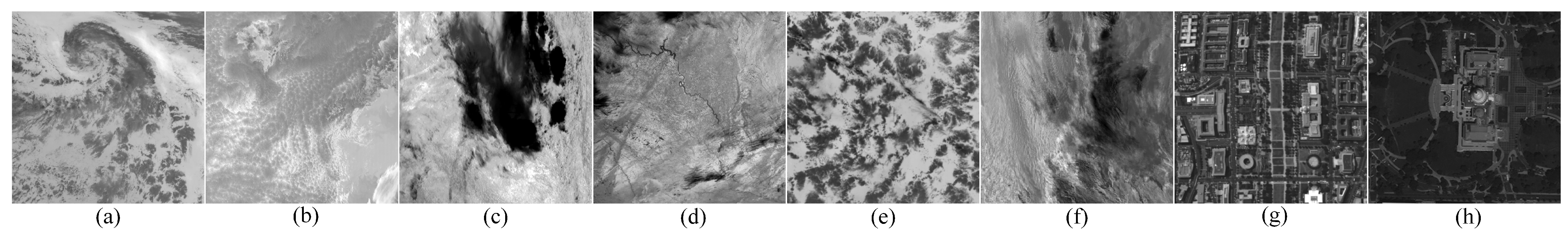
4.1.1. Experimental Environment and Data

The denoiser as well as stripe estimation models are trained in MATLAB (R2015b) environment with MatConvNet package [80] on a PC with Intel Core i7-5960X CPU 3.0 GHz 16.0 GB memory associated with a Nvidia GTX 1080Ti GPU. The test data are downloaded from [81,82,83]. In [81], the MODIS aboard Terra and Aqua level 1B data contain 36 spectral bands, in which the data of the 36th band are degraded by both stripe and AGWN noise. Hyperspectral data in [82] and multispectral data in [83] are selected to test the structure preservation ability. The selected test images are cropped to 162,752 patches of size $35\times 35$ and are separated randomly into training and test images with a ratio of 8:2.

4.1.2. Experimental Parameters Setting

The denoiser learning network is trained by using stochastic gradient descent (SGD) [84] with a learning rate of ${10}^{-4}$ and is finished after 60 epochs while the stripe estimation network is trained by employing ADAM solver [85] with a learning rate of ${10}^{-5}$ and is finished after 300 epochs. The parameter $\beta$ in Equation (23) is empirically set to 0.5. From Equation (13) to Equation (16), we can find that there are five involved parameters including two regularization parameters ${\lambda }_1$ and ${\lambda }_2$, two penalty parameters ${\mu }_1$ and ${\mu }_2$, and iteration number K to be set. Generally, the regularization parameters ${\lambda }_1$ and ${\lambda }_2$ come from the prior terms and keep fixed during iterations, and they are usually set as an empirical range for favorable performance, such as ${\lambda }_1\in \left[0.21,0.53\right]$ and ${\lambda }_2\in \left[0.19,0.57\right]$. In our experiments, we fix them to 0.25 and 0.21, respectively. Theoretically, the noise level (${\sigma }_1=\sqrt{{\lambda }_1/{\mu }_1}$ or ${\sigma }_2=\sqrt{{\lambda }_2/{\mu }_2}$) is gradually decreasing during iterations, resulting in the continuous increment of the penalty parameters ${\mu }_1$ or ${\mu }_2$. In this paper, the initial ${\sigma }_1^0$ is fixed to 29 and the final ${\sigma }_1^K$ is determined by the image noise level (which is usually less than 29) while the initial ${\sigma }_2^0$ is set to 49 and the final ${\sigma }_2^K$ is determined by the stripe’s intensity. Both ${\sigma }_1$ and ${\sigma }_2$ are uniformly sampled from the initial noise level to the final one in log space. The convergence criterion is as follows:

$$\frac{{∥x^{k+1}-x^k∥}_2^2}{{∥x^k∥}_2^2}<{\eta }_1$$

(24)

and

$$\frac{{∥s^{k+1}-s^k∥}_2^2}{{∥s^k∥}_2^2}<{\eta }_2,$$

(25)

where ${\eta }_1=3\times {10}^{-4}$ and ${\eta }_2=2\times {10}^{-4}$ in the following experiments. When the convergence criterion is not satisfied, the total iteration number K is set to 29, which is large enough to get a excited performance.

4.1.3. Compared Methods and Evaluation Indexes Selection

To verify the efficiency of the proposed D³CNNs, several state-of-the-arts derived from different categories are selected to be compared, including two-stage mixed noise removal (first denoising (Weighted Nuclear Norm Minimization, WNNM [26]), then destriping (Weighted Double-Sparsity Unidirectional Variation, WDSUV [49]) (WNNM-WDSUV), model-based methods (UTVSR [57] and JAWS [56]), semi-discrimination learning method (UV-DCNN [69]), and full-discrimination learning method (HSI-DeNet [72]). In the synthetic experiments, the synthesized RSIs are noised by AGWN ranged from 15 to 30 with a step size of 5 and stripe with three intensities (10, 30, and 50) as well as three proportions (0.1, 0.4, and 0.6), which are similar to those in Ref. [43]. Except for the visual comparisons, the objective indexes are also selected to quantitatively assess their ability of AGWN and stripe noise removal. For instance, two referenced indices, peak signal-to-noise ratio (PSNR) and structural similarity index (SSIM) [34], are employed to respectively assess the capability of noise reduction and structure preservation in synthetic experiments. While four reference-free metrics, mean of the mean relative deviation (MMRD) to evaluate the performance in retaining fine details of noise-free sharp regions [49], Q-Metric (QM) to evaluate the denoising performance [59], mean of the inverse coefficient of variation (MICV) to reflect the level of the remaining stripe noise in homogeneous regions [86], and natural image quality evaluator (NIQE) to evaluate the quality of the improved results [87], are employed for quantitative evaluation in the real-world experiments. In these indices, small MMRD and NIQE values depict that the estimated image quality is quite encouraged while large values of other metrics indicate that the results are pleasing.

In the following test experiments, eight synthetic RSIs (as shown in Figure 5) and seven real-life degraded RSIs (as shown in Figure 6) are selected to be experimented for the verification of the efficiency of the proposed D³CNNs strategy.

4.2. Discussion of Intermediate Results

Figure 7c–e and Figure 8h–j respectively provide the visual results of $x^k$ and $s^k$ at different iterations on the testing images from Figure 5, while both Figure 7f and Figure 8f show the PSNR convergence curves for $x^k$ and $s^k$. From the figures, several observations can be concluded as follows: First, the deep denoiser and the deep striper priors play the important roles of noise removal and stripe estimation, leading to a noise-free image x and a clean stripe s. Second, compared with intermediate results, the final results including x and s contain more fine details while they are more visually similar to the ground-truths, meaning that Equations (13) and (14) can iteratively recover the details with the help of two deep priors. Third, according to Figure 7f and Figure 8f, $x^k$ and $s^k$ enjoy a fast convergence to a fixed point.

4.3. Experiments on Synthetic Rsis

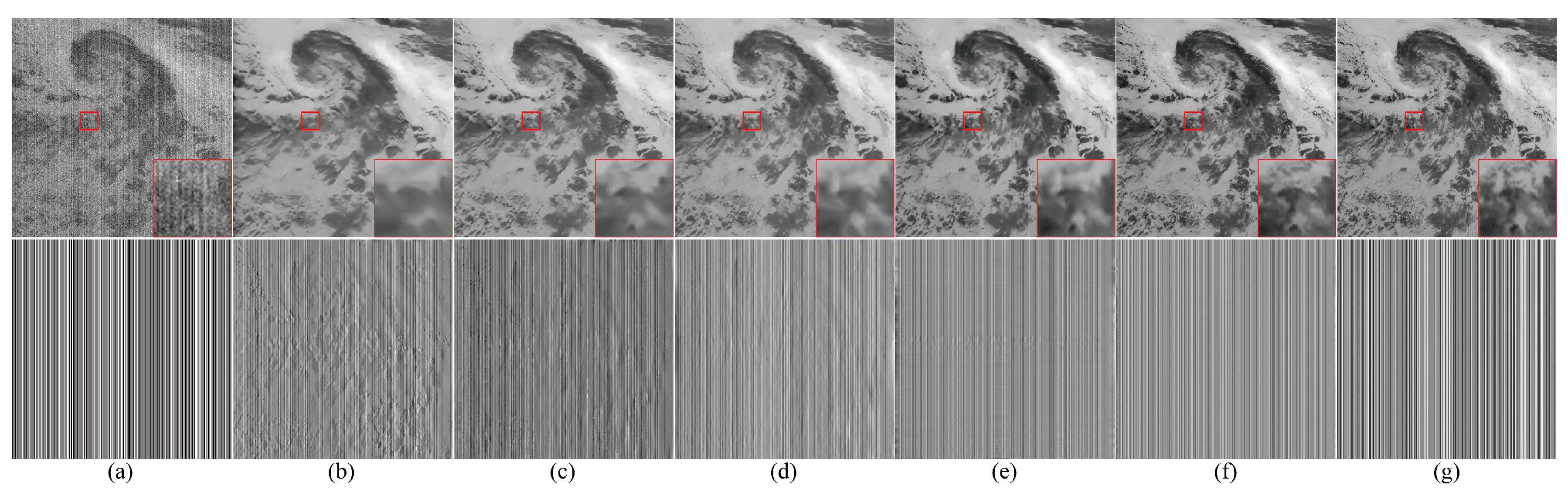
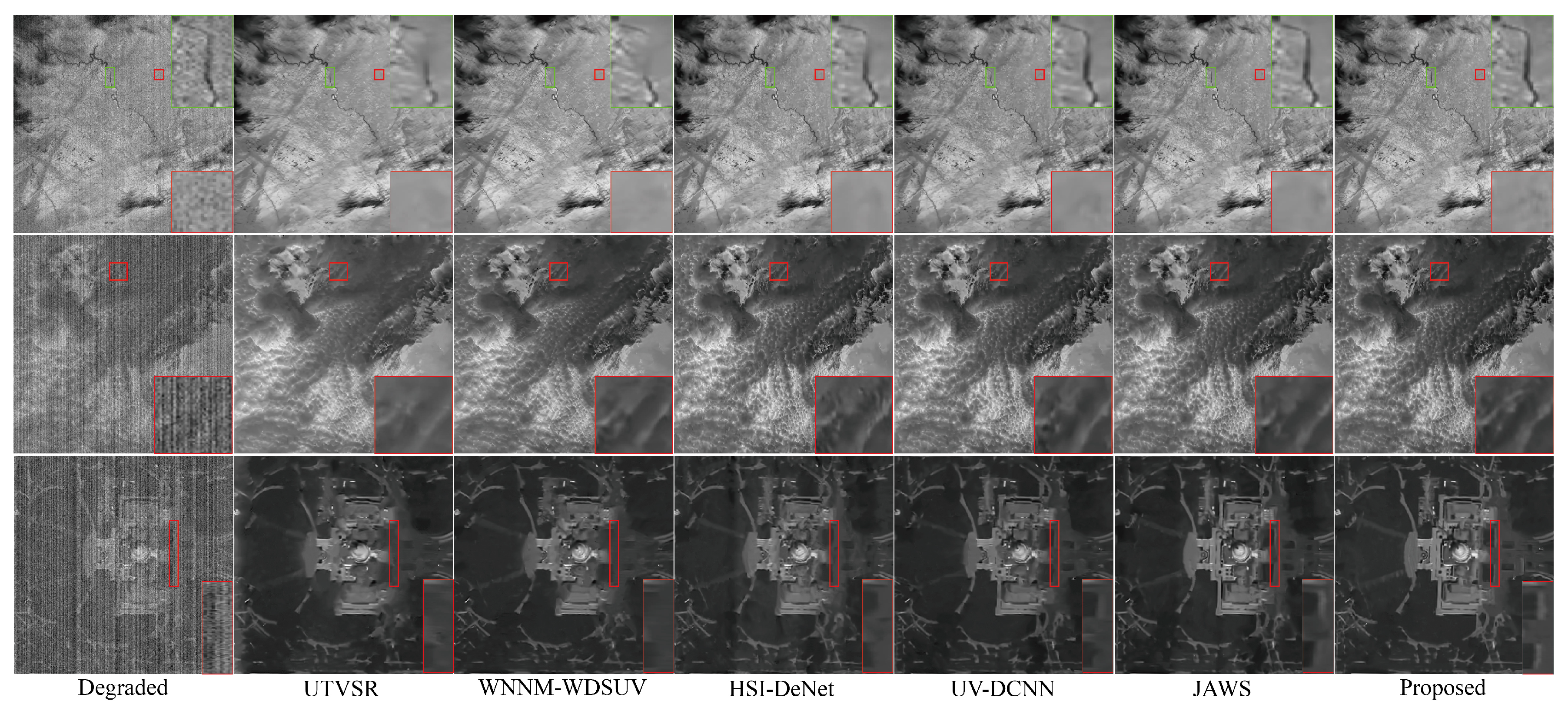
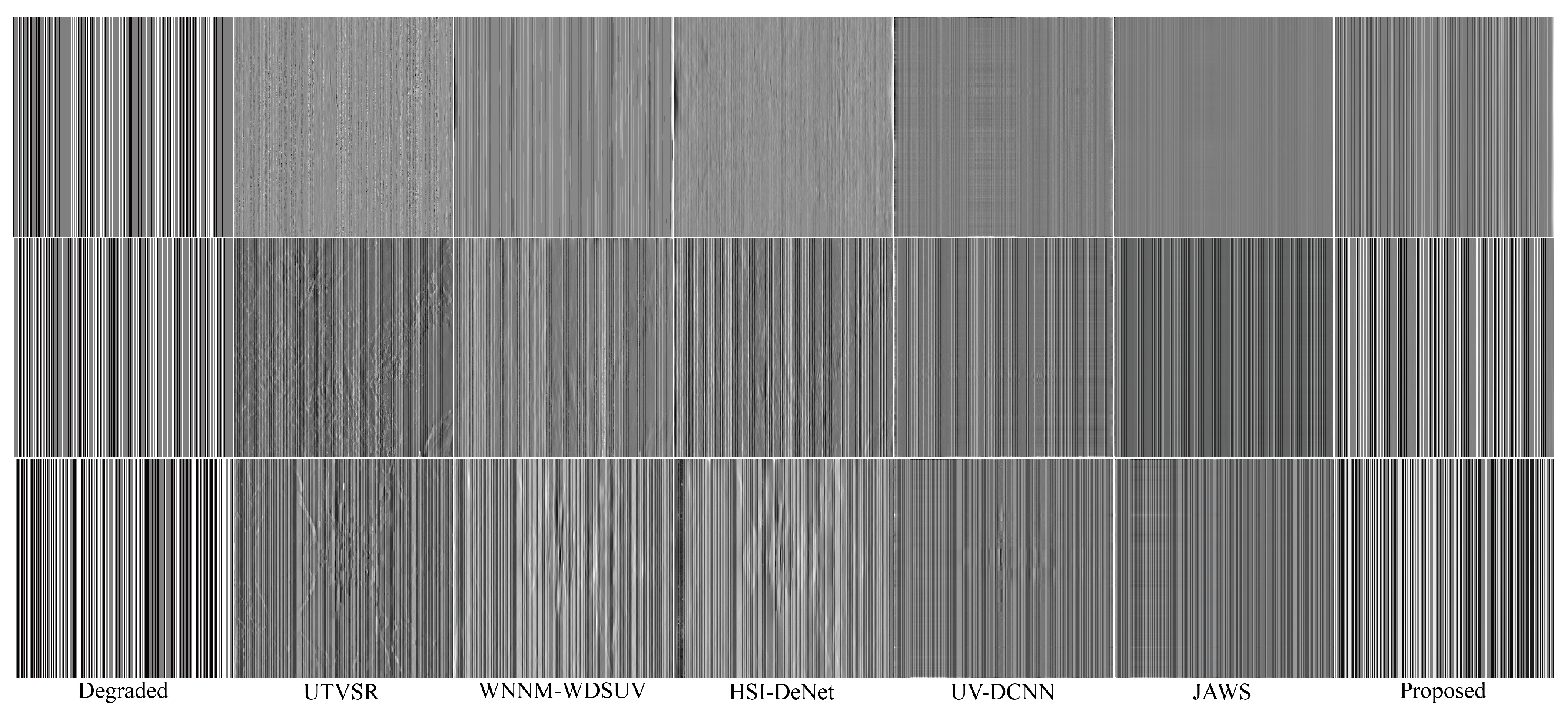
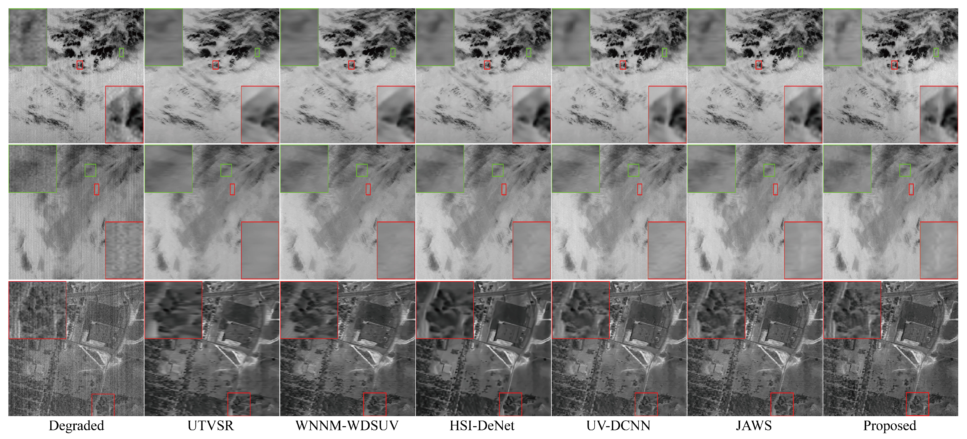
4.3.1. Qualitative Evaluation

To subjectively assess the efficiency of the D³CNNs approach, we select the visual comparisons of five synthetic RSIs degraded by AGWN with different noise level and the stripe with different types (including period, proportion, and intensity), as shown in Figure 9, Figure 10, Figure 11 and Figure 12. From the figures, we can see that all of state-of-the-arts have great ability in denoising and removing stripe. However, their performance can be discriminated from the enlarged visual areas, of which the observations can be concluded as follows: First, many fine details, especially the structures along the stripe, of the image results yielded by the UTVSR (Figure 9a, Figure 10a and Figure 11) and WNNM-WDSUV (Figure 9b, Figure 10b and Figure 11) methods are over-smoothed. Second, the HSI-DeNet method estimates latent clean images from the view of image decomposition and preserves more details than the prior two approaches but is still subject to losing image details in stripe maps, resulting in the lost of many rich details, as shown in Figure 9c, Figure 10c, Figure 11 and Figure 12. Third, the UV-DCNN method plugs the DCNN denoiser prior into the UV model, which reduces the interference of AGWN on the recovery of the stripe to a great extent. As shown in Figure 9e, Figure 10e, Figure 11 and Figure 12, the image details in stripe maps become less while the details in estimated images are richer. Fourth, with deep feature analysis of image and stripe, the JAWS method uses the characteristics of both image and stripe as constrained priors for the construction of a unified model to restore image and stripe. Compared with the forward four method, the JAWS method produces the suitable visual results with more abundant details and more comfortable stripes, as shown in Figure 9f, Figure 10f, Figure 11 and Figure 12. Finally, the proposed D³CNNs method yields better promising image and stripe results (as shown in Figure 9g, Figure 10g, Figure 11 and Figure 12) on details preservation in image and stripe regularity, illustrating that our method is better than others in image restoration.

4.3.2. Quantitative Assessment

As noise levels especially the stripe’s types are different, we employ mean PSNR (MPSNR) and mean SSIM (MSSIM) to objectively evaluate each method. Such indices are defined as follows:

$$MPSNR=\frac{1}{N}\sum _{i_1=1}^2\sum _{i_2=1}^3\sum _{i_3=1}^{3}PSNR\left(i_1,i_2,i_3\right),$$

(26)

and

$$MSSIM=\frac{1}{N}\sum _{i_1=1}^2\sum _{i_2=1}^3\sum _{i_3=1}^{3}SSIM\left(i_1,i_2,i_3\right),$$

(27)

for each image at one noise level, where $N=2\times 3\times 3=18$, $i_1=1$ represents the periodical stripe while $i_1=2$ is the non-periodical stripe. $i_2=1$, 2, and 3 respectively denote the stripe’s intensity as 10, 30, and 50 while $i_3=1$, 2, and 3 respectively represent the stripe’s proportion as 0.1, 0.4, and 0.6. Quantitative MPSNR and MSSIM results are respectively compared in

Table 1. Quantitative MPSNR comparisons of the state-of-the-arts on the synthetic optical RSIs shown in Figure 5.

Methods	STM1				STM2				STM3
	$\sigma =15$	$\sigma =20$	$\sigma =25$	$\sigma =30$	$\sigma =15$	$\sigma =20$	$\sigma =25$	$\sigma =30$	$\sigma =15$	$\sigma =20$	$\sigma =25$	$\sigma =30$
UTVSR	28.14	26.86	25.9	25.22	29.96	28.83	27.58	27.1	33.12	32.04	31.05	30.25
WNNM-WDSUV	28.82	27.52	26.62	25.94	30.91	29.63	28.75	28.09	34.55	33.42	32.61	31.98
HSI-DeNet	29.02	27.71	26.77	26.04	31.02	29.72	28.78	28.1	34.71	33.56	32.72	32.08
UV-DCNN	29.05	27.77	26.89	26.24	31.13	29.87	29	28.34	34.78	33.6	32.84	32.11
JAWS	29.24	27.86	26.93	26.25	31.21	29.93	29.03	28.36	34.86	33.71	32.93	32.28
Proposed	29.68	28.15	27.46	26.76	31.59	30.47	29.73	28.69	35.18	34.06	33.38	32.79
Methods	SAM1				SAM2				SAM3
	$\sigma =15$	$\sigma =20$	$\sigma =25$	$\sigma =30$	$\sigma =15$	$\sigma =20$	$\sigma =25$	$\sigma =30$	$\sigma =15$	$\sigma =20$	$\sigma =25$	$\sigma =30$
UTVSR	28.67	27.14	25.98	25.21	28.46	27.13	26.02	25.29	28.12	26.92	26.11	25.27
WNNM-WDSUV	29.31	27.75	26.62	25.74	29.25	27.81	26.84	26.09	29.01	27.74	26.88	26.25
HSI-DeNet	29.24	27.77	26.68	25.82	29.36	27.98	26.95	26.14	29.17	27.88	26.98	26.29
UV-DCNN	29.47	28.01	26.89	26	29.45	28.11	27.14	26.4	29.31	27.97	27.13	26.5
JAWS	29.52	27.99	26.82	25.97	29.58	28.18	27.2	26.44	29.32	28.05	27.17	26.52
Proposed	29.75	28.64	27.33	26.47	30.02	28.83	27.91	27.08	29.84	28.68	27.79	27.01
Methods	SWDCM				SWDCM
	$\sigma =15$	$\sigma =20$	$\sigma =25$	$\sigma =30$	$\sigma =15$		$\sigma =20$		$\sigma =25$		$\sigma =30$
UTVSR	28.53	27	25.68	24.8	31.03		29.71		28.85		28.33
WNNM-WDSUV	29.44	27.76	26.51	25.53	32.41		30.96		29.87		29.03
HSI-DeNet	29.5	27.91	26.72	25.75	32.61		31.2		30.06		29.16
UV-DCNN	29.52	27.87	26.57	25.69	32.69		31.27		30.26		29.27
JAWS	29.62	28.02	26.77	25.84	32.83		31.41		30.33		29.48
Proposed	29.84	28.33	27.06	26.37	33.17		31.76		30.8		29.97

and

Table 2. Quantitative MSSIM comparisons of the state-of-the-arts on the synthetic optical RSIs shown in Figure 5.

Methods	STM1				STM2				STM3
	$\sigma =15$	$\sigma =20$	$\sigma =25$	$\sigma =30$	$\sigma =15$	$\sigma =20$	$\sigma =25$	$\sigma =30$	$\sigma =15$	$\sigma =20$	$\sigma =25$	$\sigma =30$
UTVSR	0.7872	0.7251	0.6626	0.6205	0.815	0.7592	0.7118	0.6825	0.8766	0.8587	0.8482	0.8342
WNNM-WDSUV	0.8196	0.7748	0.7209	0.6842	0.8237	0.7734	0.7476	0.7149	0.8821	0.872	0.8567	0.8413
HSI-DeNet	0.8216	0.7843	0.7257	0.6861	0.832	0.7771	0.7471	0.7157	0.8826	0.8715	0.8559	0.8424
UV-DCNN	0.8466	0.7944	0.7318	0.6898	0.8433	0.782	0.7482	0.7179	0.8895	0.8728	0.8577	0.8426
JAWS	0.8472	0.8003	0.7356	0.6917	0.8482	0.7867	0.7488	0.7187	0.8919	0.8724	0.8585	0.8462
Proposed	0.8518	0.8126	0.7415	0.7172	0.8527	0.8037	0.7524	0.7318	0.9011	0.8829	0.8617	0.8534
Methods	SAM1				SAM2				SAM3
	$\sigma =15$	$\sigma =20$	$\sigma =25$	$\sigma =30$	$\sigma =15$	$\sigma =20$	$\sigma =25$	$\sigma =30$	$\sigma =15$	$\sigma =20$	$\sigma =25$	$\sigma =30$
UTVSR	0.8908	0.8524	0.8216	0.7913	0.805	0.7249	0.6452	0.5886	0.748	0.6772	0.5981	0.5562
WNNM-WDSUV	0.8998	0.8662	0.8312	0.806	0.8127	0.7615	0.7094	0.6753	0.7846	0.7179	0.6661	0.6229
HSI-DeNet	0.905	0.8646	0.8335	0.8054	0.8225	0.7648	0.7137	0.6783	0.7763	0.7178	0.6673	0.6243
UV-DCNN	0.8996	0.8676	0.8309	0.8096	0.8266	0.7737	0.7168	0.6802	0.794	0.7196	0.6718	0.6277
JAWS	0.9064	0.8698	0.8334	0.8073	0.8272	0.7755	0.7155	0.6793	0.7992	0.7192	0.6728	0.6283
Proposed	0.9172	0.8813	0.8594	0.8216	0.8353	0.7962	0.7367	0.7015	0.8127	0.7533	0.7119	0.6527
Methods	SWDCM				SWDCM
	$\sigma =15$	$\sigma =20$	$\sigma =25$	$\sigma =30$	$\sigma =15$		$\sigma =20$		$\sigma =25$		$\sigma =30$
UTVSR	0.8912	0.8241	0.7802	0.7384	0.861		0.8287		0.7807		0.7477
WNNM-WDSUV	0.8937	0.8486	0.8094	0.7808	0.8645		0.83		0.7971		0.7725
HSI-DeNet	0.9003	0.8525	0.8123	0.7832	0.8619		0.8319		0.7976		0.7743
UV-DCNN	0.8978	0.8539	0.8139	0.7858	0.8651		0.8468		0.8066		0.7805
JAWS	0.9014	0.8549	0.8145	0.7833	0.8647		0.8476		0.8079		0.7817
Proposed	0.9153	0.8792	0.8386	0.8124	0.8878		0.8629		0.8237		0.8019

, from which the following two conclusions are involved: (1) for each image, both MPSNR and MSSIM are decreasing along with the increment of noise level, the larger noise level will seriously contaminate the images, making it more difficulty in the estimated results being closer to ground-truth. (2) The proposed D³CNNs approach generates the highest MPSNR and MSSIM values on each image at the same noise level, illustrating that it is effective and even better than the state-of-the-arts, which is consistent with visual comparisons.

Run time, an important index to assess the efficiency of algorithms, is tested on images with different sizes, the results of which are shown in

Table 3. Average computation time (Unit: Seconds) comparison on different image size. For learning-based methods, the computation times on CPU/GPU are both presented.

Image Size	Methods
	UTVSR	WNNM-WDSUV	HSI-DeNet	UV-DCNN	JAWS	Proposed
$256\times 256$	653.923	108.714	1.048/0.016	1.077/0.035	874.675	1.068/0.024
$512\times 512$	2674.641	440.283	5.869/0.027	7.953/0.142	2937.424	6.667/0.073

. From the table, we can find several observations: First, the run time of the discriminative learning methods (the results are marked with color font), even in the CPU version, is faster than that of the model-based optimization approaches. Second, the pure discriminative learning (HSI-DeNet, its results are marked with red font) gets the fastest speed on either CPU or GPU version under the same image size, which is reasonable and is used to learn a specialized prior (such as denoiser prior in UV-DCNN, the results are marked with green font) to be plugged into the model-based optimization methods for improving the computation time and boosting the modeling ability. Third, with the help of two deep priors, the proposed D³CNNs generates the second fastest runtime, which is a little slower than that of HSI-DeNet, but it has much better MPSNR (as shown in Table 1) and MSSIM (as shown in Table 2) than HSI-DeNet.

According to the comprehensive consideration of the comparable results, we can get that D³CNNs is a flexible and faithful method for image restoration.

4.4. Applications to the Real-World Degraded Rsis

To further verify the efficiency of the proposed D³CNNs scheme, we apply it to the real-world degraded RSIs shown in Figure 6 and compare it to state-of-the-arts qualitatively and quantitatively. The visual comparisons of the estimated images and the calculated stripe maps are respectively shown in Figure 13 and Figure 14, from which we can find that the details of images produced by our method are richer while the stripes are cleaner and more regular than those produced by others. Such conclusions denote that the results decomposed by our method are more faithful and are closer to original clean maps including images and stripes.

Table 4. Quantitative comparisons of the state-of-the-arts on the real-life optical RSIs shown in Figure 6.

Indexes	Methods	RAM1	RAM2	RAM3	RTM1	RTM2	RTM3	Urban
QM	UTVSR	25.18	32.37	11.82	12.57	12.83	23.78	27.58.
	WNNM-WDSUV	25.47	32.69	12.24	13.08	13.26	24.33	28.81
	HSI-DeNet	26.39	33.97	12.89	13.67	13.81	24.85	30.49
	UV-DCNN	26.62	34.57	13.48	14.13	14.37	25.61	31.14
	JAWS	26.79	34.78	14.17	14.52	14.88	25.94	31.63
	Proposed	27.11	35.27	14.72	15.18	15.49	26.37	32.16
MICV	UTVSR	35.72	33.26	38.19	37.54	36.47	36.79	29.46
	WNNM-WDSUV	35.91	33.67	38.42	37.76	36.65	36.92	29.58
	HSI-DeNet	36.15	33.83	38.79	37.93	36.89	37.27	29.84
	UV-DCNN	36.29	34.08	38.94	38.17	37.09	37.55	30.09
	JAWS	36.67	34.41	39.18	38.54	37.51	37.86	30.57
	Proposed	36.86	34.74	39.49	38.82	37.74	38.28	31.07
MMRD	UTVSR	0.45	0.67	0.051	0.058	0.062	0.36	0.57
	WNNM-WDSUV	0.39	0.52	0.046	0.051	0.055	0.32	0.53
	HSI-DeNet	0.37	0.049	0.041	0.047	0.048	0.29	0.48
	UV-DCNN	0.33	0.041	0.037	0.042	0.043	0.27	0.44
	JAWS	0.29	0.036	0.031	0.036	0.038	0.22	0.35
	Proposed	0.21	0.026	0.022	0.027	0.029	0.19	0.27
NIQE	UTVSR	7.03	7.37	4.18	4.22	4.26	6.73	7.19
	WNNM-WDSUV	6.94	7.18	4.05	4.11	4.17	6.67	7.07
	HSI-DeNet	6.81	7.06	3.94	4.08	4.09	6.51	6.91
	UV-DCNN	6.67	6.84	3.78	3.83	3.85	6.17	6.39
	JAWS	6.46	6.61	3.62	3.67	3.71	5.95	6.08
	Proposed	6.23	6.33	3.28	3.36	3.39	5.28	5.62

For each image, the best result is marked with bold font.

shows the comparisons of quantitative results generated by the state-of-the-arts, from which several observations can be concluded: First, all of them yield considerable QM values, illustrating that they perform well on denoising. Our method produces the highest QM value for each RSI, showing the strongest ability of rich detail preservation. Then, the small difference of MICV values on the same RSI represents that they are all well in stripe removal in homogeneous regions. Meanwhile, for the same RSI, our method produces the smallest MMRD value, reflecting that it can generate pleasing results with more fine details in noise-free sharp regions. Finally, the smallest NIQE value obtained by our method on the same RSI demonstrates that it can better improve the image quality than others.

In sum, the comparisons of quantitative associated with qualitative results contribute to validate the effectiveness of the proposed D³CNNs method.

5. Conclusions

Random noise (additive Gaussian white noise, AGWN) as well as stripe noise always coexists in remotely sensed images, increasing the difficulty in constructing the inverse problems. To cope with this problem and preserve as more details as possible in estimated remotely sensed image, this paper had proposed a novel dual denoiser driven convolutional neural networks (D³CNNs) which has the following key points: (1) two deep learning networks are trained for different specialized tasks, specially denoising and stripe estimation. (2) The prelearned modules are respectively employed as denoiser and striper priors plugged into the model-based optimization method of HQS to solve the image restoration problem. Experimental results had validated that the two deep powerful priors can improve the effective of model-based methods, with which the proposed D³CNNs strategy yields quite competitive visual and quantitative results compared to the state-of-the-arts. The satisfactory run time is suitable for further applications. Although the proposed method performs well on mixed noise removal (main for two additive noise), it is still to be further extended to reduce other noise, such as impulse noise and Poisson noise.

References

- Li, Y.; Chen, W.; Zhang, Y.; Tao, C.; Xiao, R.; Tan, Y. Accurate cloud detection in high-resolution remote sensing imagery by weakly supervised deep learning. Remote Sens. Environ. 2020, 250, 112045. [Google Scholar] [CrossRef]
- Li, Y.; Zhang, Y.; Huang, X.; Zhu, H.; Ma, J. Large-scale remote sensing image retrieval by deep hashing neural networks. IEEE Trans. Geosci. Remote Sens. 2018, 56, 950–965. [Google Scholar] [CrossRef]
- Li, Y.; Kong, D.; Zhang, Y.; Tan, Y.; Chen, L. Robust deep alignment network with remote sensing knowledge graph for zero-shot and generalized zero-shot remote sensing image scene classification. ISPRS JPRS 2021, 179, 145–158. [Google Scholar] [CrossRef]
- Li, Y.; Zhou, Y.; Zhang, Y.; Zhong, L.; Wang, J.; Chen, J. DKDFN: Domain knowledge-guided deep collaborative fusion network for multimodal unitemporal remote sensing land cover classification. ISPRS JPRS 2022, 186, 170–189. [Google Scholar] [CrossRef]
- Li, Y.; Chen, W.; Huang, X.; Gao, Z.; Li, S.; He, T.; Zhang, Y. Mfvnet: Deep adaptive fusion network with multiple field-of-views for remote sensing image semantic segmentation. Sci. China Inf. Sci. 2022. [Google Scholar] [CrossRef]
- Huang, Z.; Zhang, Y.; Li, Q.; Zhang, T.; Sang, N.; Hong, H. Progressive dual-domain filter for enhancing and denoising optical remote sensing images. IEEE Geosci. Remote Sens. Lett. 2018, 15, 759–763. [Google Scholar] [CrossRef]
- Chang, Y.; Chen, M.; Yan, L.; Zhao, X.; Li, Y.; Zhong, S. Toward universal stripe removal via wavelet-based deep convolutional neural network. IEEE Trans. Geosci. Remote Sens. 2020, 58, 2880–2897. [Google Scholar] [CrossRef]
- Rudin, L.I.; Osher, S.; Fatemi, E. Nonlinear total variation based noise removal algorithms. Physica D 1992, 60, 259–268. [Google Scholar] [CrossRef]
- Han, L.; Zhao, Y.; Lv, H.; Zhang, Y.; Liu, H.; Bi, G. Remote Sensing Image Denoising Based on Deep and Shallow Feature Fusion and Attention Mechanism. Remote Sens. 2022, 14, 1243. [Google Scholar] [CrossRef]
- Zhang, B.; Aziz, Y.; Wang, Z.; Zhuang, L.; Michael, K.N.; Gao, L. Hyperspectral Image Stripe Detection and Correction Using Gabor Filters and Subspace Representation. IEEE Geosci. Remote Sens. Lett. 2022, 19, 1–5. [Google Scholar] [CrossRef]
- Sun, L.; He, C.; Zheng, Y.; Wu, Z.; Jeon, B. Tensor Cascaded-Rank Minimization in Subspace: A Unified Regime for Hyperspectral Image Low-Level Vision. IEEE Trans. Image Process. 2023, 32, 100–115. [Google Scholar] [CrossRef]
- Yu, Y.; Samaki, B.; Rashidi, M.; Mohammadi, M.; Nguyen, T.; Zhang, G. Vision-based concrete crack detection using a hybrid framework considering noise effect. J. Build. Eng. 2022, 61, 105246. [Google Scholar] [CrossRef]
- Syam, T.; Muthalif, A. Magnetorheological Elastomer based torsional vibration isolator for application in a prototype drilling shaft. J. Low Freq. Noise Vib. Act. Control 2022, 41, 676–700. [Google Scholar] [CrossRef]
- Chambolle, A. An algorithm for total variation minimization and applications. J. Math. Imag. Vis. 2004, 20, 89–97. [Google Scholar]
- Chan, T.F.; Esedoglu, S. Aspects of total variation regularized li function approximation. SIAM J. Appl. Math. 2005, 65, 1817–1837. [Google Scholar] [CrossRef]
- Osher, S.; Burger, M.; Goldfarb, D.; Xu, J.; Yin, W. An iterative regularization method for total variation-based image restoration. Multiscale Model. Simul. 2005, 4, 460–489. [Google Scholar] [CrossRef]
- Peyre, G.; Bougleux, S.; Cohen, L.D. Non-local regularization of inverse problems. Inverse Probl. Imaging 2011, 5, 511–530. [Google Scholar] [CrossRef]
- Condat, L. Semi-local total variation for regularization of inverse problems. In Proceedings of the 2014 22nd European Signal Processing Conference (EUSIPCO), Lisbon, Portugal, 1–5 September 2014; pp. 1806–1810. [Google Scholar]
- Jidesh, P.; Shivarama, H.K. Non-local total variation regularization models for image restoration. Comput. Electr. Eng. 2018, 67, 114–133. [Google Scholar] [CrossRef]
- Elad, M.; Aharon, M. Image denoising via sparse and redundant representations over learned dictionaries. IEEE Trans. Image Process. 2006, 15, 3736–3745. [Google Scholar] [CrossRef]
- Mairal, J.; Elad, M.; Sapiro, G. Sparse representation for color image restoration. IEEE Trans. Image Process. 2008, 17, 53–69. [Google Scholar] [CrossRef]
- Mairal, J.; Bach, F.; Ponce, J.; Sapiro, G.; Zisserman, A. Non-local sparse models for image restoration. In Proceedings of the IEEE 12th International Conference on Computer Vision, ICCV 2021, Montreal, QC, Canada, 10–17 October 2021; pp. 2272–2279. [Google Scholar]
- Dong, W.; Zhang, L.; Shi, G.; Li, X. Nonlocally centralized sparse representation for image restoration. IEEE Trans. Image Process. 2013, 22, 1620–1630. [Google Scholar] [CrossRef] [PubMed]
- Dong, W.; Shi, G.; Ma, Y.; Li, X. Image restoration via simultaneous sparse coding: Where structured sparsity meets Gaussian scale mixture. Int. J. Comput. Vis. (IJCV) 2015, 114, 217–232. [Google Scholar] [CrossRef]
- Huang, Z.; Li, Q.; Zhang, T.; Sang, N.; Hong, H. Iterative weighted sparse representation for X-ray cardiovascular angiogram image denoising over learned dictionary. IET Image Process. 2018, 12, 254–261. [Google Scholar] [CrossRef]
- Gu, S.; Zhang, L.; Zuo, W.; Feng, X. Weighted nuclear norm minimization with application to image denoising. In Proceedings of the 2014 IEEE Conference on Computer Vision and Pattern Recognition, Columbus, OH, USA, 23–28 June 2014; pp. 2862–2869. [Google Scholar]
- Xie, Y.; Gu, S.; Liu, Y.; Zuo, W.; Zhang, W.; Zhang, L. Weighted schatten p-norm minimization for image denoising and background subtraction. IEEE Trans. Image Process. 2016, 25, 4842–4857. [Google Scholar] [CrossRef]
- Wu, Z.; Wang, Q.; Jin, J.; Shen, Y. Structure tensor total variation-regularized weighted nuclear norm minimization for hyperspectral image mixed denoising. Signal Process. 2017, 131, 202–219. [Google Scholar] [CrossRef]
- Huang, Z.; Li, Q.; Fang, H.; Zhang, T.; Sang, N. Iterative weighted nuclear norm for X-ray cardiovascular angiogram image denoising. Signal Image Video Process. 2017, 11, 1445–1452. [Google Scholar] [CrossRef]
- Huang, T.; Dong, W.; Xie, X.; Shi, G.; Bai, X. Mixed Noise Removal via Laplacian Scale Mixture Modeling and Nonlocal Low-Rank Approximation. IEEE Trans. Image Process. 2017, 26, 3171–3186. [Google Scholar] [CrossRef] [PubMed]
- Yao, S.; Chang, Y.; Qin, X.; Zhang, Y.; Zhang, T. Principal component dictionary-based patch grouping for image denoising. J. Vis. Commun. Image Represent. 2018, 50, 111–122. [Google Scholar] [CrossRef]
- Chen, Y.; Pock, T. Trainable nonlinear reaction diffusion: A flexible framework for fast and effective image restoration. IEEE Trans. Pattern Anal. Mach. Intell. 2017, 39, 1256–1272. [Google Scholar] [CrossRef]
- Zhang, K.; Zuo, W.; Chen, Y.; Meng, D.; Zhang, L. Beyond a Gaussian denoiser: Residual learning of deep CNN for image denoising. IEEE Trans. Image Process. 2017, 26, 3142–3155. [Google Scholar] [CrossRef]
- Zhang, K.; Zuo, W.; Gu, S.; Zhang, L. Learning deep CNN denoiser prior for image restoration. In Proceedings of the IEEE Conference on Computer Vision and Pattern Recognition (CVPR), Honolulu, HI, USA, 21–26 July 2017; pp. 2808–2817. [Google Scholar]
- Zhang, K.; Zuo, W.; Zhang, L. FFDNet: Toward a fast and flexible solution for CNN-based image denoising. IEEE Trans. Image Process. 2018, 27, 4608–4622. [Google Scholar] [CrossRef] [PubMed]
- Tai, Y.; Yang, J.; Liu, X.; Xu, C. MemNet: A persistent memory network for image restoration. In Proceedings of the IEEE International Conference on Computer Vision, Venice, Italy, 22–29 October 2017; pp. 4549–4557. [Google Scholar]
- Scetbon, M.; Elad, M.; Milanfar, P. Deep K-SVD Denoising. IEEE Trans. Image Process. 2021, 30, 5944–5955. [Google Scholar] [CrossRef] [PubMed]
- Zhang, H.; Yong, H.; Zhang, L. Deep convolutional dictionary learning for image denoising. In Proceedings of the Computer Vision and Pattern Recognition (CVPR), Nashville, TN, USA, 20–25 June 2021; pp. 630–641. [Google Scholar]
- Carfantan, H.; Idier, J. Statistical linear destriping of satellite-based pushbroom-type images. IEEE Trans. Geosci. Remote Sens. 2010, 48, 1860–1872. [Google Scholar] [CrossRef]
- Fehrenbach, J.; Weiss, P.; Lorenzo, C. Variational algorithms to remove stationary noise: Applications to microscopy imaging. IEEE Trans. Image Process. 2012, 21, 860–1871. [Google Scholar] [CrossRef]
- Liu, X.; Lu, X.; Shen, H.; Yuan, Q.; Jiao, Y.; Zhang, L. Stripe noise separation and removal in remote sensing images by consideration of the global sparsity and local variational properties. IEEE Trans. Image Process. 2016, 54, 3049–3060. [Google Scholar] [CrossRef]
- Liu, X.; Lu, X.; Shen, H.; Yuan, Q.; Zhang, L. Oblique stripe removal in remote sensing images via oriented variation. arXiv 2018, arXiv:1809.02043. [Google Scholar]
- Chang, Y.; Yan, L.; Wu, T.; Zhong, S. Remote sensing image stripe noise removal: From image decomposition perspective. IEEE Trans. Geosci. Remote Sens. 2016, 54, 7018–7031. [Google Scholar] [CrossRef]
- Chang, Y.; Yan, L.; Zhong, S. Transformed low-rank model for line pattern noise removal. In Proceedings of the IEEE International Conference on Computer Vision (ICCV), Venice, Italy, 22–29 October 2017; pp. 1726–1734. [Google Scholar]
- Chang, Y.; Yan, L.; Chen, B.; Zhong, S.; Tian, Y. Hyperspectral image restoration: Where does the low-rank property exist. IEEE Trans. Geosci. Remote Sens. 2021, 59, 6869–6884. [Google Scholar] [CrossRef]
- Chen, Y.; Huang, T.-Z.; Zhao, X.L.; Deng, L.J.; Huang, J. Stripe noise removal of remote sensing images by total variation regularization and group sparsity constraint. Remote Sens. 2017, 9, 559. [Google Scholar] [CrossRef]
- Chen, Y.; Huang, T.-Z.; Deng, L.J.; Zhao, X.-L.; Wang, M. Group sparsity based regularization model for remote sensing image stripe noise removal. Neurocomputing 2017, 267, 95–106. [Google Scholar] [CrossRef]
- Cao, W.; Chang, Y.; Han, G.; Li, J. Destriping remote sensing image via low-rank approximation and nonlocal total variation. IEEE Geosci. Remote Sens. Lett. 2018, 15, 848–852. [Google Scholar] [CrossRef]
- Song, Q.; Wang, Y.; Yan, X.; Gu, H. Remote sensing images stripe noise removal by double sparse regulation and region separation. Remote Sens. 2018, 10, 998. [Google Scholar] [CrossRef]
- Dhivya, R.; Prakash, R. Stripe noise separation and removal in remote sensing images. J. Comput. Theor. Nanosci. 2018, 15, 2724–2728. [Google Scholar] [CrossRef]
- Cui, H.; Jia, P.; Zhang, G.; Jiang, Y.; Li, L.; Wang, J.; Hao, X. Multiscale intensity propagation to remove multiplicative stripe noise from remote sensing images. IEEE Trans. Geosci. Remote Sens. 2020, 58, 2308–2323. [Google Scholar] [CrossRef]
- Kuang, X.; Sui, X.; Chen, Q.; Gu, G. Single infrared image stripe noise removal using deep convolutional networks. IEEE Photonics J. 2017, 9, 1–13. [Google Scholar] [CrossRef]
- Xiao, P.; Guo, Y.; Zhuang, P. Removing stripe noise from infrared cloud images via deep convolutional networks. IEEE Photonics J. 2018, 10, 1–14. [Google Scholar] [CrossRef]
- Zhong, Y.; Li, W.; Wang, X.; Jin, S.; Zhang, L. Satellite-ground intergraded destriping network: A new perspective for eo-1 hyperion and chinese hyperspectral satellite datasets. Remote Sens. Environ. 2020, 237, 111416. [Google Scholar] [CrossRef]
- Song, J.; Jeong, H.-H.; Park, D.-S.; Kim, H.-H.; Seo, D.-C.; Ye, J.C. Unsupervised denoising for satellite imagery using wavelet directional cyclegan. IEEE Trans. Geosci. Remote Sens. 2020, 59, 6823–6839. [Google Scholar] [CrossRef]
- Huang, Z.; Zhang, Y.; Li, Q.; Li, X.; Zhang, T.; Sang, N.; Hong, H. Joint analysis and weighted synthesis sparsity priors for simultaneous denoising and destriping optical remote sensing images. IEEE Trans. Geosci. Remote Sens. 2020, 58, 6958–6982. [Google Scholar] [CrossRef]
- Chang, Y.; Yan, L.; Fang, H.; Liu, H. Simultaneous destriping and denoising for remote sensing images with unidirectional total variation and sparse representation. IEEE Geosci. Remote Sens. Lett. 2014, 11, 1051–1055. [Google Scholar] [CrossRef]
- Xiong, F.; Zhou, J.; Qian, Y. Hyperspectral restoration via L0 gradient regularized low-rank tensor factorization. IEEE Geosci. Remote Sens. Lett. 2019, 57, 10410–10425. [Google Scholar] [CrossRef]
- Zheng, Y.; Huang, T.; Zhao, X.; Jiang, T.; Ma, T.; Ji, T. Mixed noise removal in hyperspectral image via low-fibered-rank regularization. IEEE Trans. Geosci. Remote Sens. 2020, 58, 734–749. [Google Scholar] [CrossRef]
- Liu, L.; Xu, L.; Fang, H. Simultaneous intensity bias estimation and stripe noise removal in infrared images using the global and local sparsity constraints. IEEE Trans. Geosci. Remote Sens. 2020, 58, 1777–1789. [Google Scholar] [CrossRef]
- Zeng, H.; Xie, X.; Cui, H.; Yin, H.; Ning, J. Hyperspectral image restoration via global L1−2 spatial-spectral total variation regularized local low-rank tensor recovery. IEEE Trans. Geosci. Remote Sens. 2020, 59, 3309–3325. [Google Scholar] [CrossRef]
- Xie, T.; Li, S.; Sun, B. Hyperspectral images denoising via nonconvex regularized low-rank and sparse matrix decomposition. IEEE Trans. Image Process. 2020, 29, 44–56. [Google Scholar] [CrossRef]
- Hu, T.; Li, W.; Liu, N.; Tao, R.; Zhang, F.; Scheunders, P. Hyperspectral image restoration using adaptive anisotropy total variation and nuclear norms. IEEE Trans. Geosci. Remote Sens. 2021, 59, 1516–1533. [Google Scholar] [CrossRef]
- Wang, M.; Wang, Q.; Chanussot, J.; Hong, D. l0 − l1 Hybrid total variation regularization and its applications on hyperspectral image mixed noise removal and compressed sensing. IEEE Trans. Geosci. Remote Sens. 2021, 59, 7695–7710. [Google Scholar] [CrossRef]
- Wang, S.; Zhu, Z.; Zhao, R.; Zhang, B. Hyperspectral image denoising via nonconvex logarithmic penalty. Math. Probl. Eng. 2021, 2021, 5535169. [Google Scholar] [CrossRef]
- Dong, W.; Zuo, W.; Zhang, D.; Zhang, L.; Yang, M.H. Simultaneous fidelity and regularization learning for image restoration. arXiv 2019, arXiv:1804.04522v4. [Google Scholar]
- Dong, W.; Wang, P.; Yin, W.; Shi, G.; Wu, F.; Lu, X. Denoising prior driven deep neural network for image restoration. IEEE Trans. Pattern Anal. Mach. Intell. (TPAMI) 2019, 41, 2305–2318. [Google Scholar] [CrossRef]
- Zhang, K.; Li, Y.; Zuo, W.; Zhang, L.; Timofte, R. Plug-and-play image restoration with deep denoiser prior. IEEE Trans. Pattern Anal. Mach. Intell. (TPAMI) 2021, 44, 6360–6376. [Google Scholar] [CrossRef] [PubMed]
- Huang, Z.; Zhang, Y.; Li, Q.; Li, Z.; Zhang, T.; Sang, N.; Xiong, S. Unidirectional variation and deep CNN denoiser priors for simultaneously destriping and denoising optical remote sensing images. Int. J. Remote Sens. 2019, 40, 5737–5748. [Google Scholar] [CrossRef]
- Zeng, H.; Xie, X.; Cui, H.; Yin, H.; Zhao, Y.; Ning, J. Hyperspectral image restoration via CNN denoiser prior regularized low-rank tensor recovery. Comput. Vis. Image Unders. 2020, 197–198, 103004. [Google Scholar] [CrossRef]
- He, Z.; Cao, Y.; Dong, Y.; Yang, J.; Cao, Y.; Tisse, C.-L. Single-image-based non-uniformity correction of uncooled long-wave infrared detectors: A deep-learning approach. Appl. Opt. 2018, 57, D155–D164. [Google Scholar] [CrossRef] [PubMed]
- Chang, Y.; Yan, L.; Fang, H.; Zhong, S.; Liao, W. HSI-DeNet: Hyperspectral image restoration via convolutional neural network. IEEE Trans. Geosci. Remote Sens. 2018, 57, 667–682. [Google Scholar] [CrossRef]
- Zhang, Q.; Yuan, Q.; Li, J.; Liu, X.; Shen, H.; Zhang, L. Hybrid noise removal in hyperspectral imagery with a spatial-spectral gradient network. IEEE Trans. Geos. Remote Sens. 2019, 57, 7317–7329. [Google Scholar] [CrossRef]
- Luo, Y.; Zhao, X.; Jiang, T.; Zheng, Y.; Chang, Y. Unsupervised hyperspectral mixed noise removal via spatial-spectral constrained deep image prior. arXiv 2021, arXiv:2008.09753. [Google Scholar] [CrossRef]
- Liu, H.; Fang, S.; Zhang, Z.; Li, D.; Lin, K.; Wang, J. MFDNet: Collaborative poses perception and matrix fisher distribution for head pose estimation. IEEE Trans. Multimed. 2021, 24, 2449–2460. [Google Scholar] [CrossRef]
- Ronneberger, O.; Fischer, P.; Brox, T. U-net: Convolutional networks for biomedical image segmentation. In Proceedings of the International Conference on Medical Image Computing and Computer-Assisted Intervention, Munich, Germany, 5–9 October 2015; pp. 234–241. [Google Scholar]
- Zhang, Y.; Yuan, L.; Wang, Y.; Zhang, J. SAU-Net: Efficient 3D spine MRI segmentation using inter-slice attention. Proc. Mach. Learn. Res. 2020, 121, 903–913. [Google Scholar]
- Yong, H.; Huang, J.; Meng, D.; Hua, X.; Zhang, L. Momentum batch normalization for deep learning with small batch size. In Proceedings of the European Conference on Computer Vision, Glasgow, UK, 23–28 August 2020; pp. 224–240. [Google Scholar]
- He, K.; Zhang, X.; Ren, S.; Sun, J. Deep residual learning for image recognition. In Proceedings of the IEEE Conference on Computer Vision and Pattern Recognition, Las Vegas, NV, USA, 27–30 June 2016; pp. 770–778. [Google Scholar]
- Vedaldi, A.; Lenc, K. MatConvNet: Convolutional neural networks for matlab. In Proceedings of the 23rd ACM Conference on Multimedia Conference, Brisbane, Australia, 26–30 October 2015; pp. 689–692. [Google Scholar]
- MODIS Data. Available online: https://modis.gsfc.nasa.gov/data/ (accessed on 30 January 2018).
- A Freeware Multispectral Image Data Analysis System. Available online: https://engineering.purdue.edu/~biehl/MultiSpec/hyperspectral.html (accessed on 30 January 2018).
- Gloabal Digital Product Sample. Available online: http://www.digitalglobe.com/product-samples (accessed on 30 January 2018).
- Tsuruoka, Y.; Tsujii, J.; Ananiadou, S. Stochastic gradient descent training for L1-regularized log-linear models with cumulative penalty. In Proceedings of the ACL 2009 the 47th Annual Meeting of the Association for Computational Linguistics and the 4th International Joint Conference on Natural Language Processing of the AFNLP, Singapore, 2–7 August 2009; pp. 477–485. [Google Scholar]
- Kingma, D.P.; Ba, J. Adam: A method for stochastic optimization. arXiv 2015, arXiv:1412.6980. [Google Scholar]
- Nichol, J.E.; Vohora, V. Noise over water surfaces in Landsat TM images. Int. J. Remote Sens. 2010, 25, 2087–2093. [Google Scholar] [CrossRef]
- Mittal, A.; Soundararajan, R.; Bovik, A.C. Making a ‘completely blind’ image quality analyzer. IEEE Signal Process. Lett. 2013, 20, 209–212. [Google Scholar] [CrossRef]