

A Google Earth Engine-Based Framework to Identify Patterns and Drivers of Mariculture Dynamics in an Intensive Aquaculture Bay in China


Abstract
1. Introduction
2. Materials and Methodology
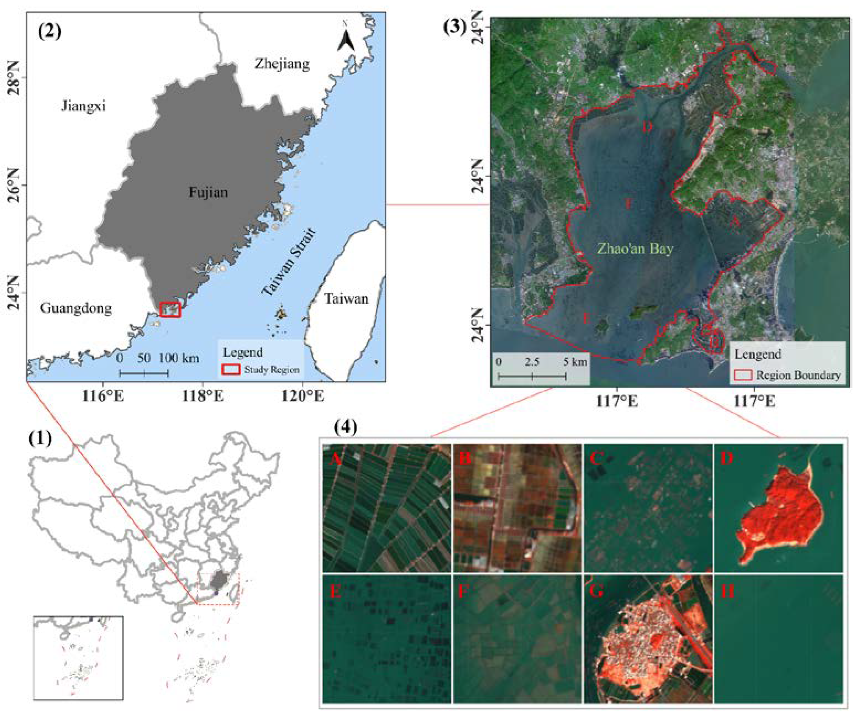
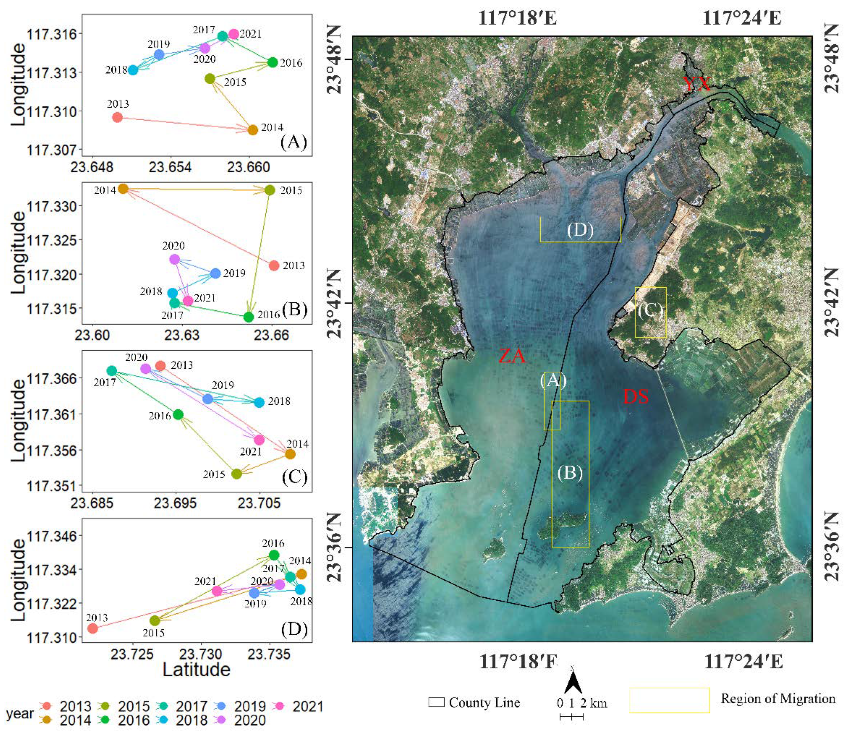
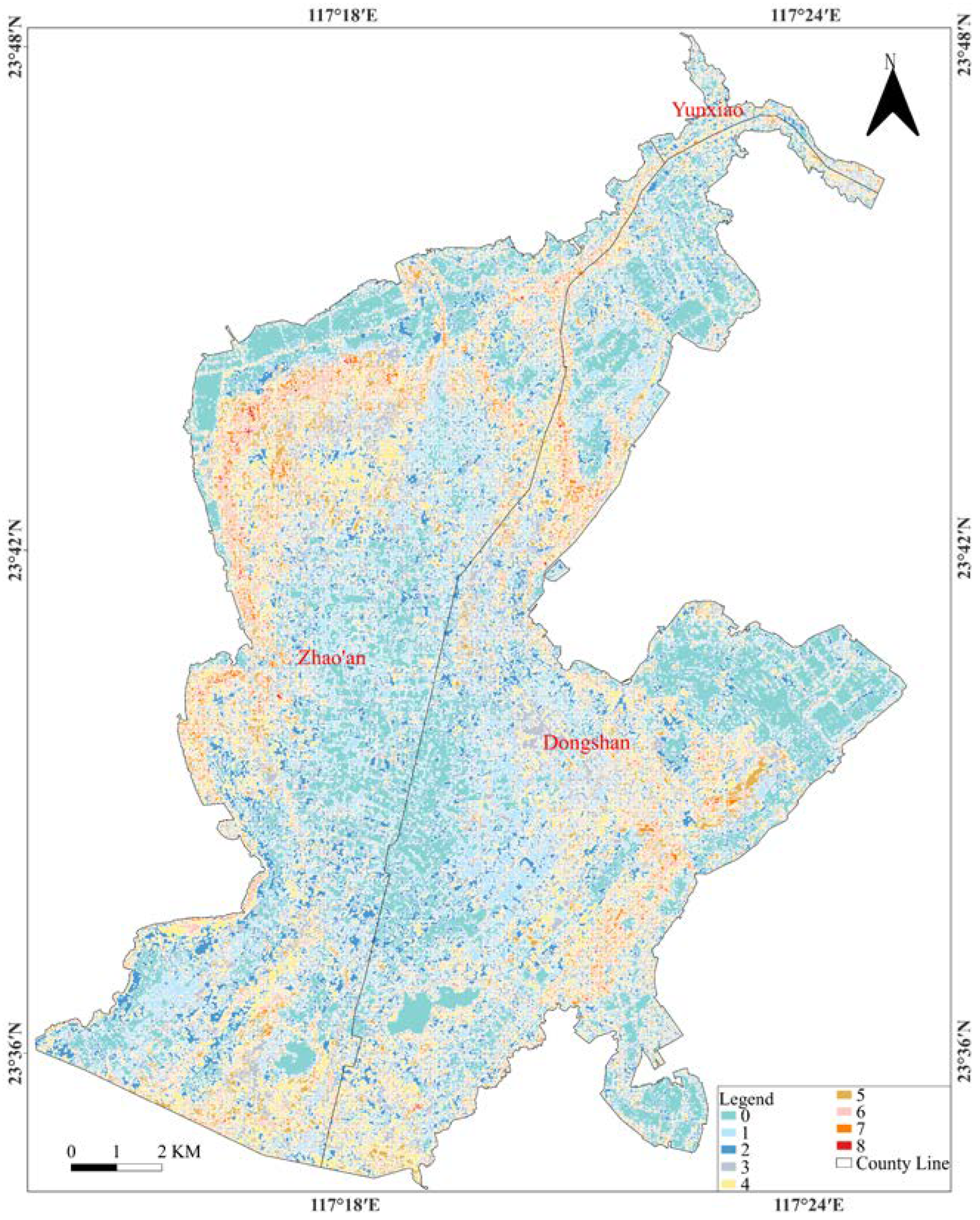
2.1. Study Area
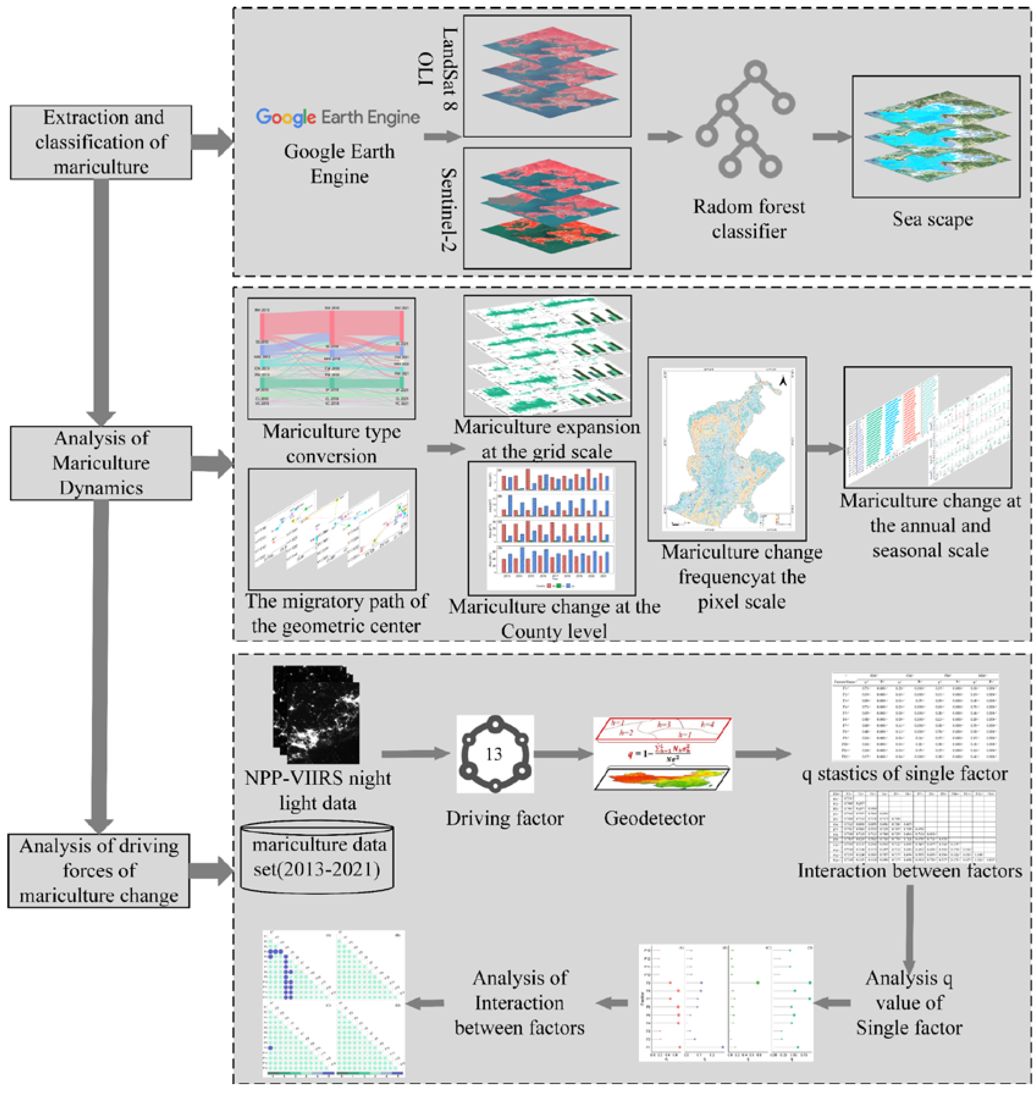
2.2. Methods
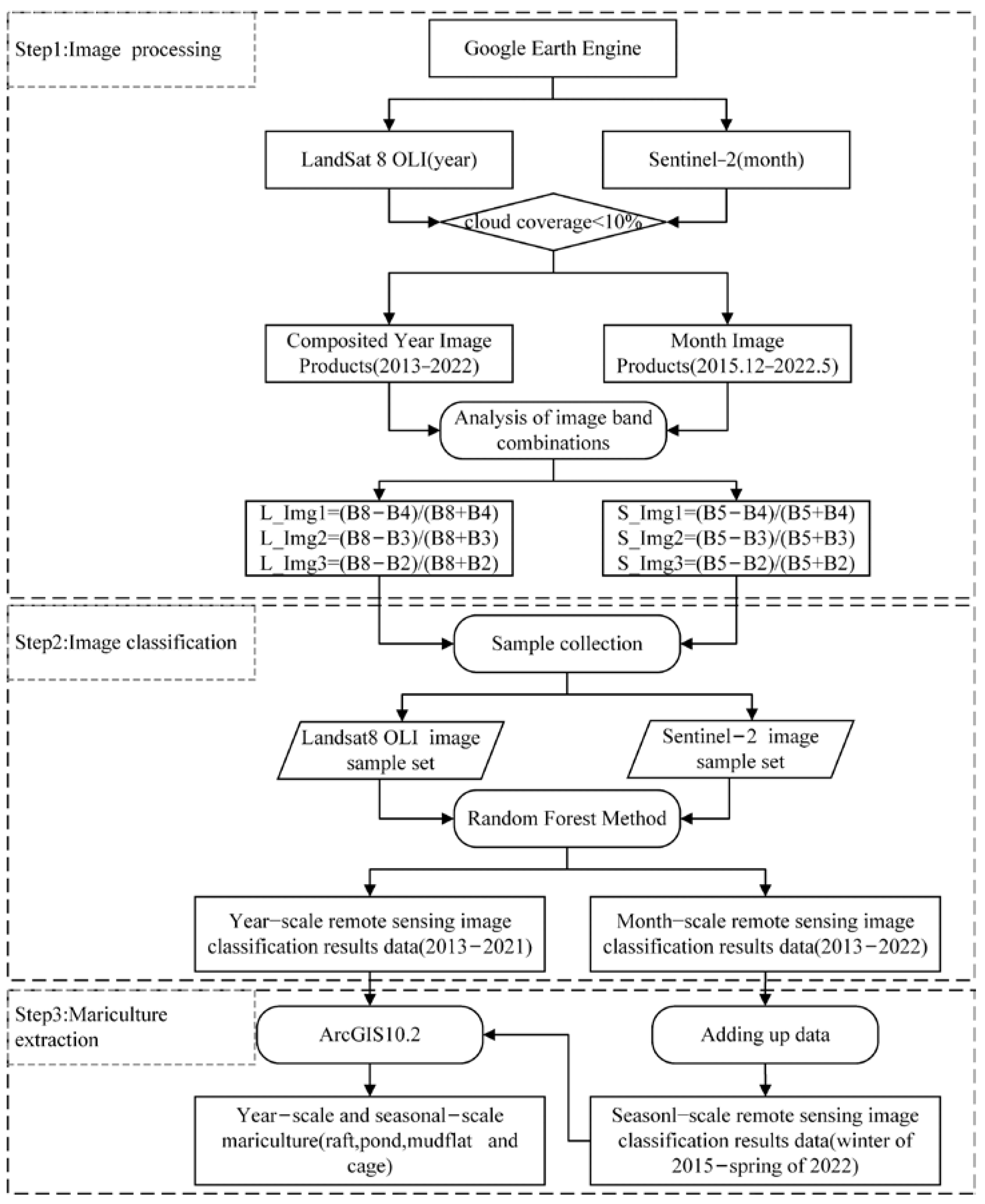
2.2.1. Extraction and Classification of Mariculture
2.2.2. Analysis of Mariculture Dynamics
2.2.3. Analysis of Driving Forces of Mariculture Change
2.3. Data Sources
3. Results
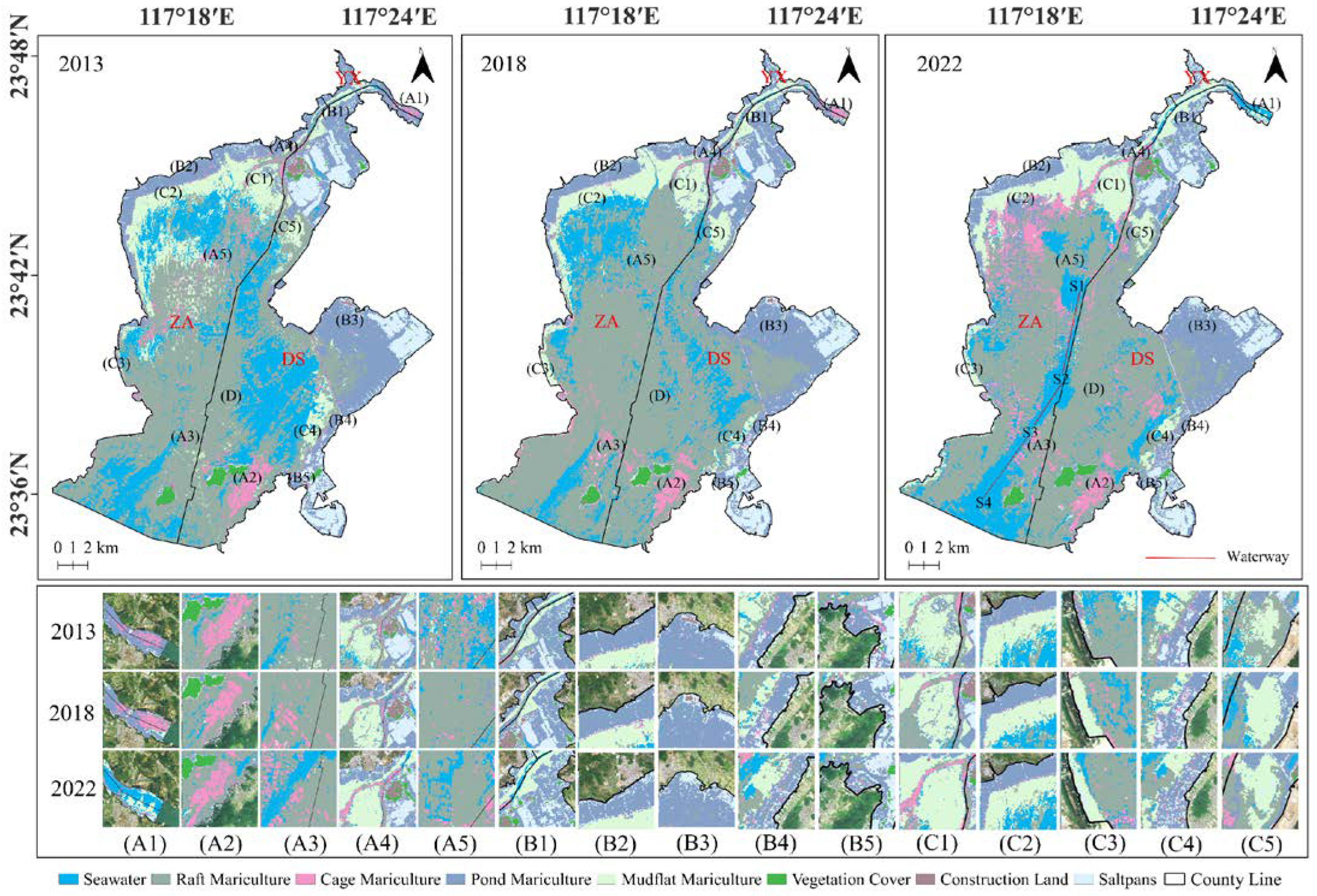
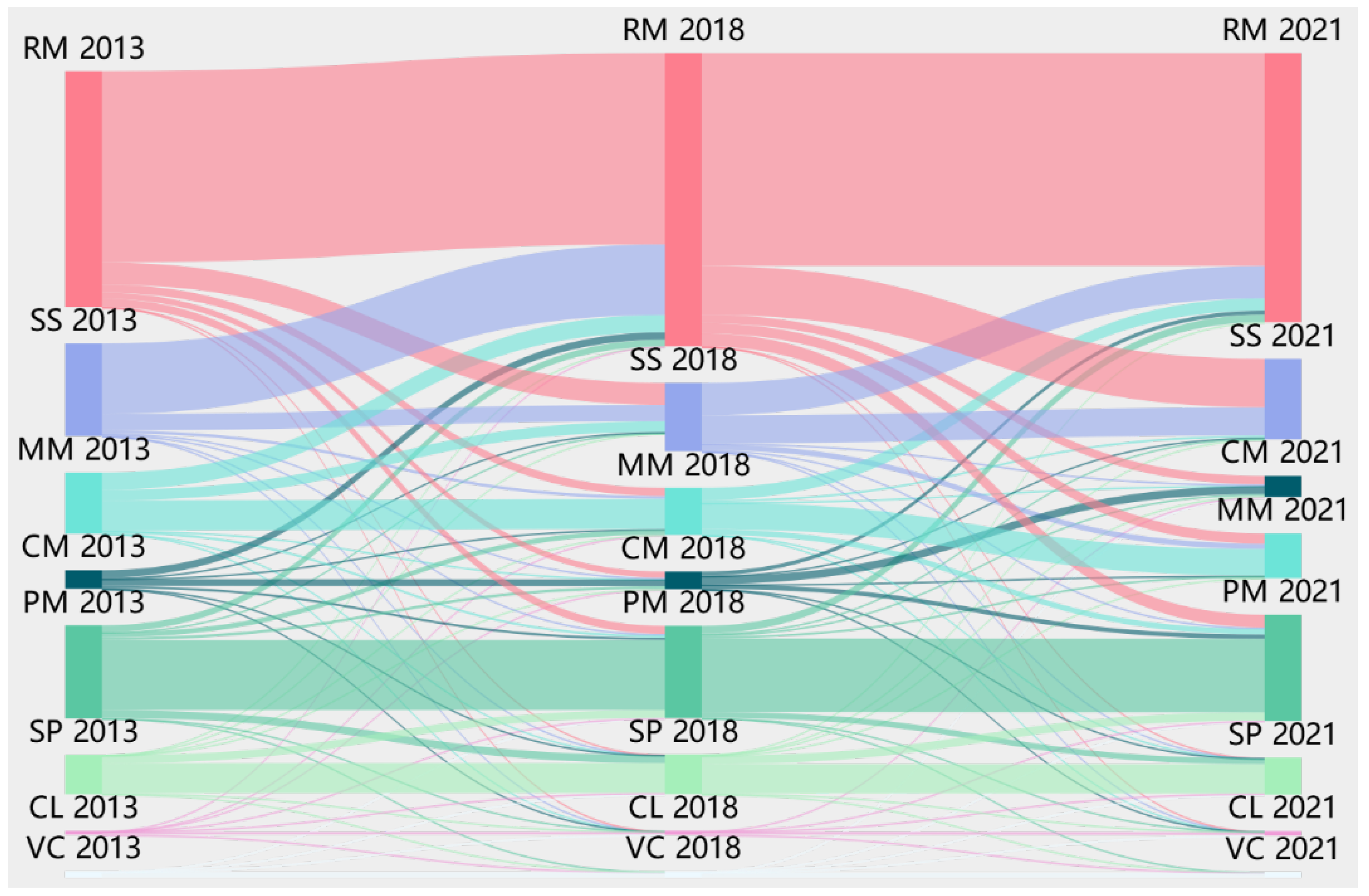
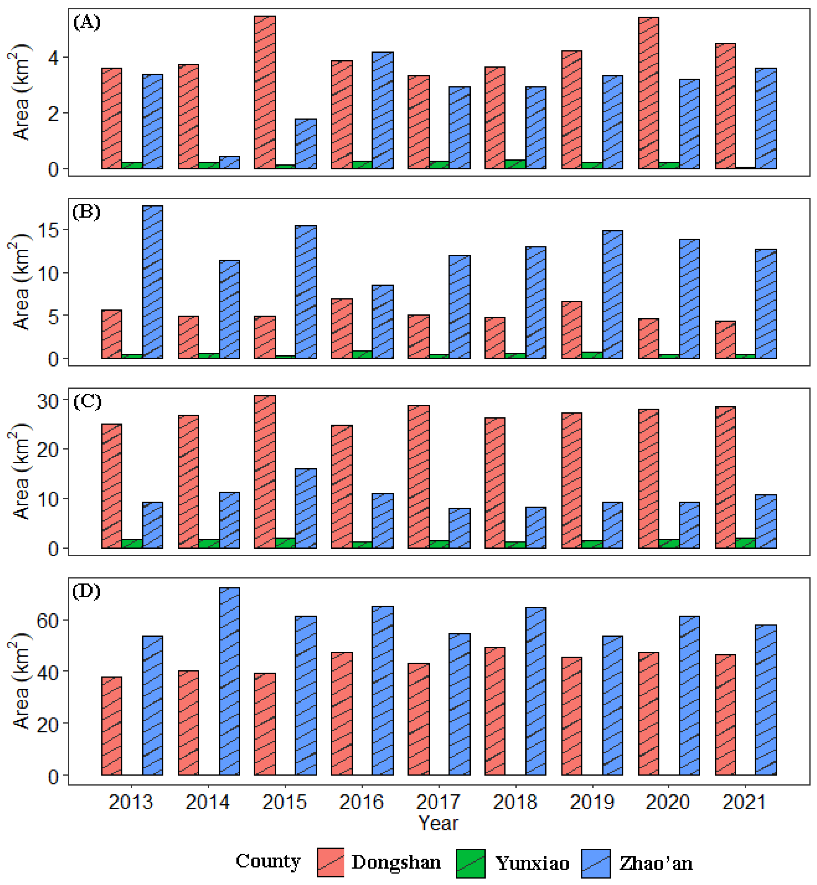
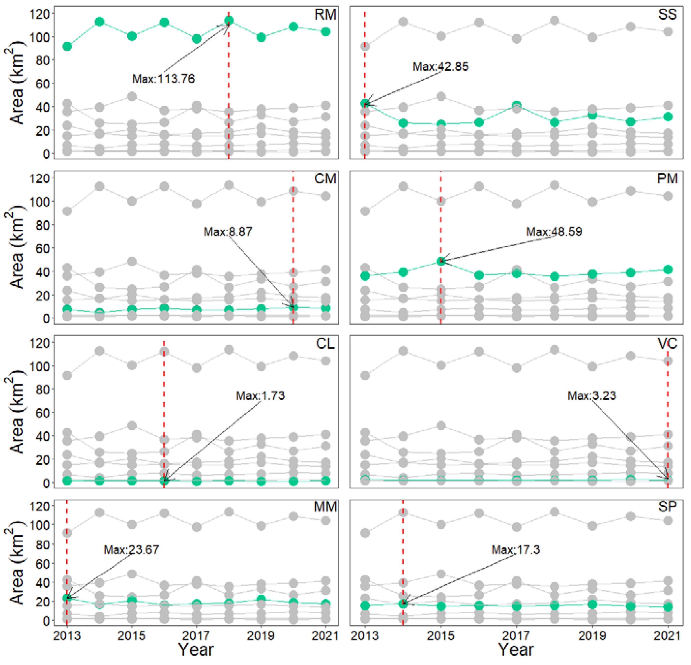
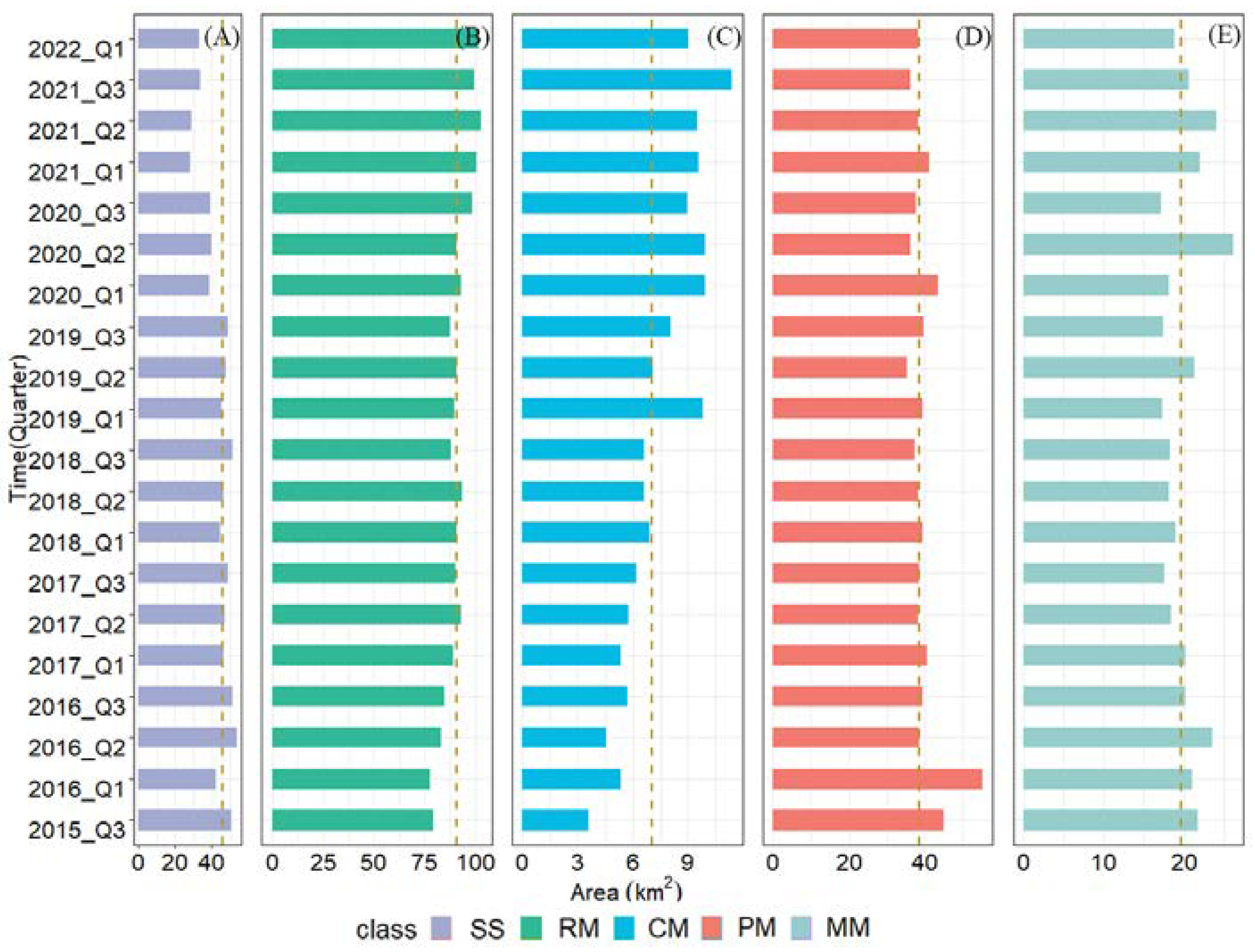
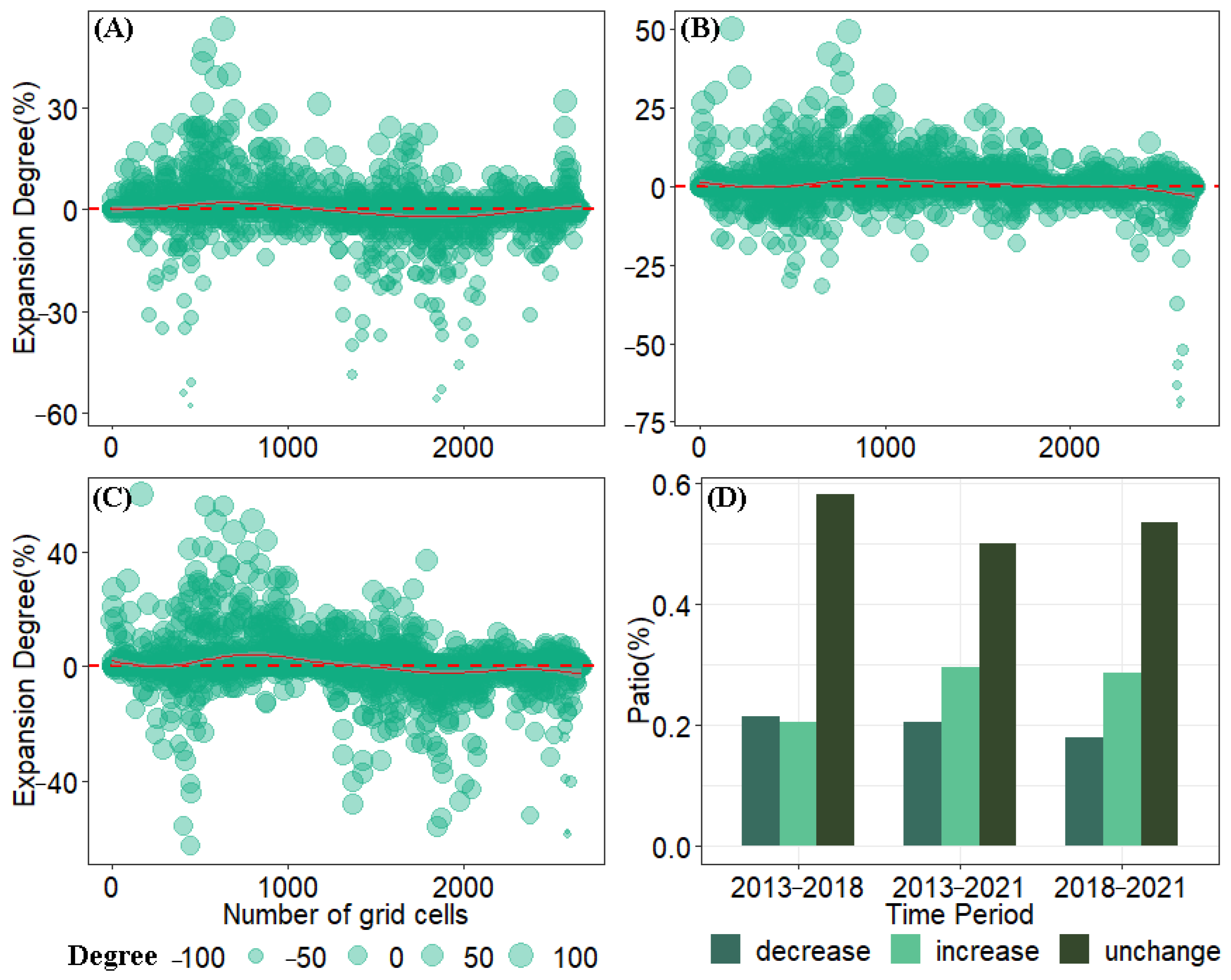
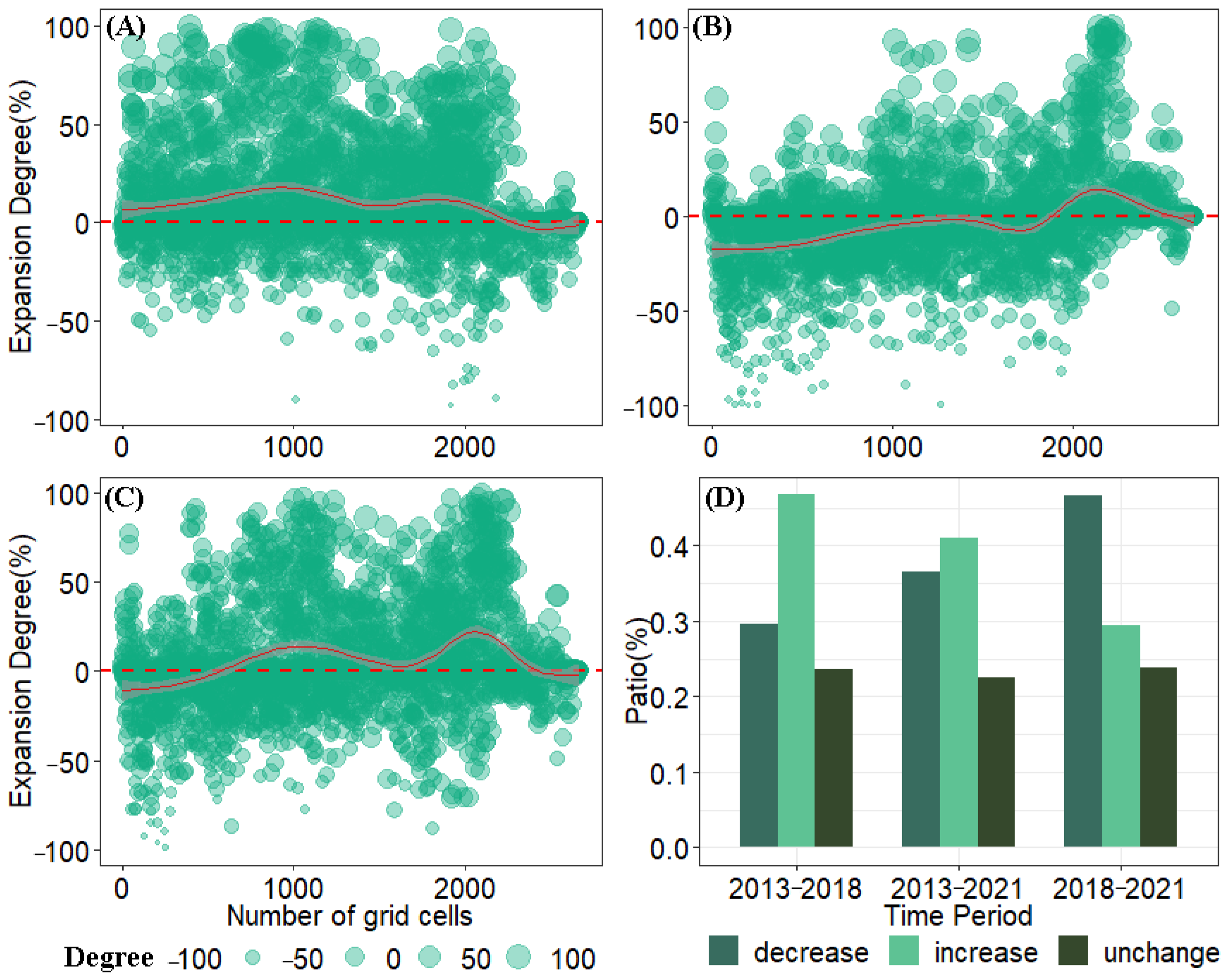
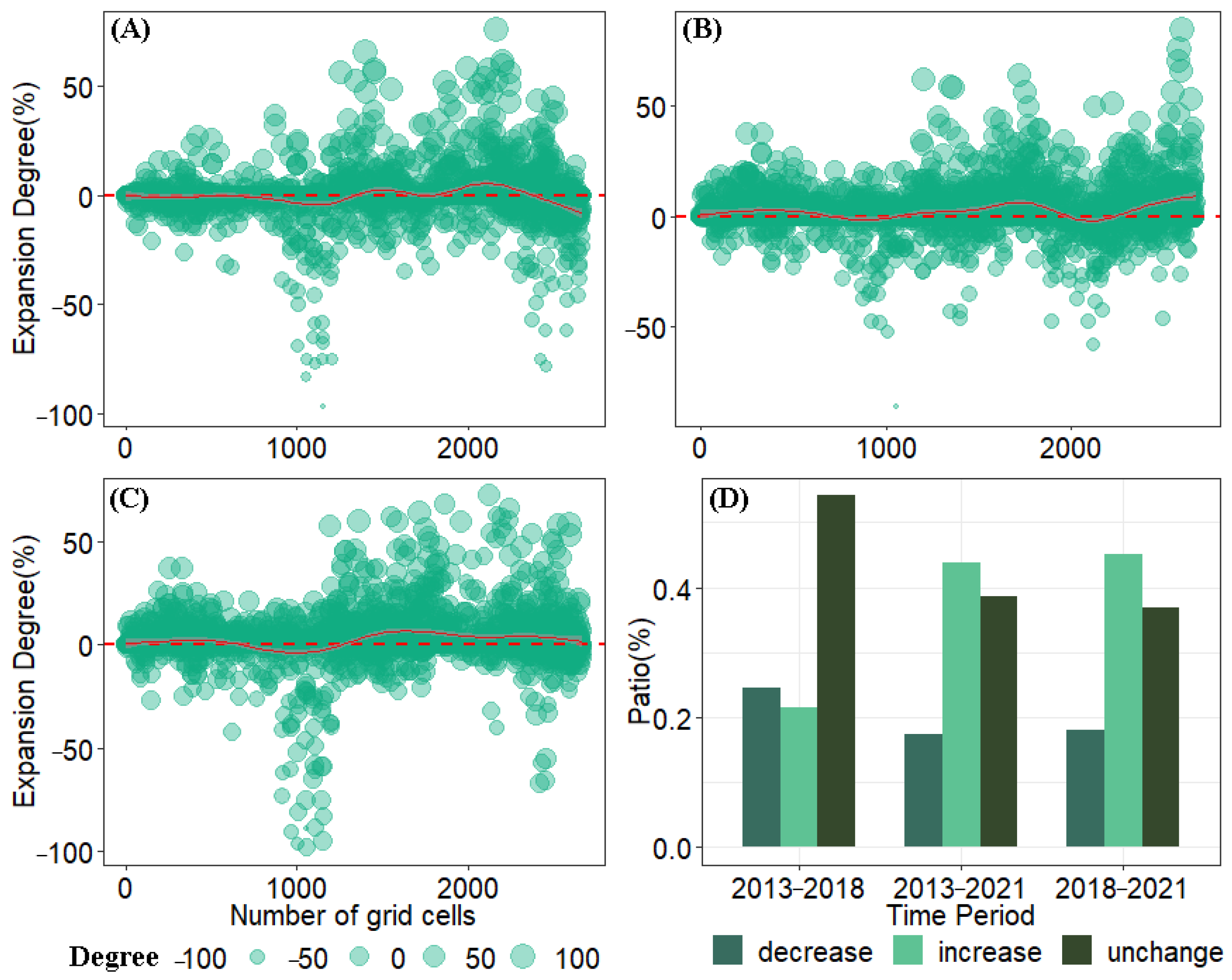
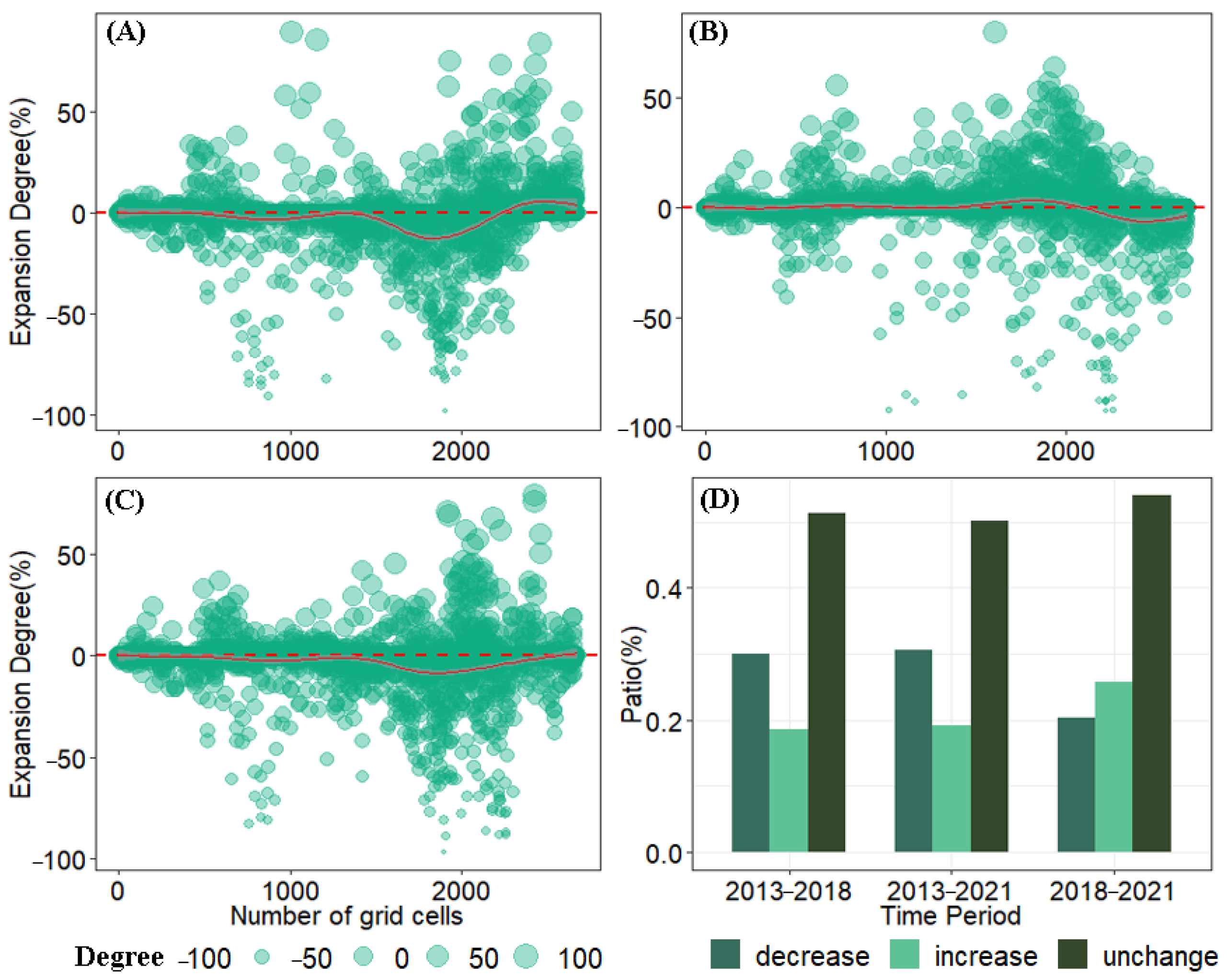
3.1. Spatiotemporal Dynamics in Mariculture
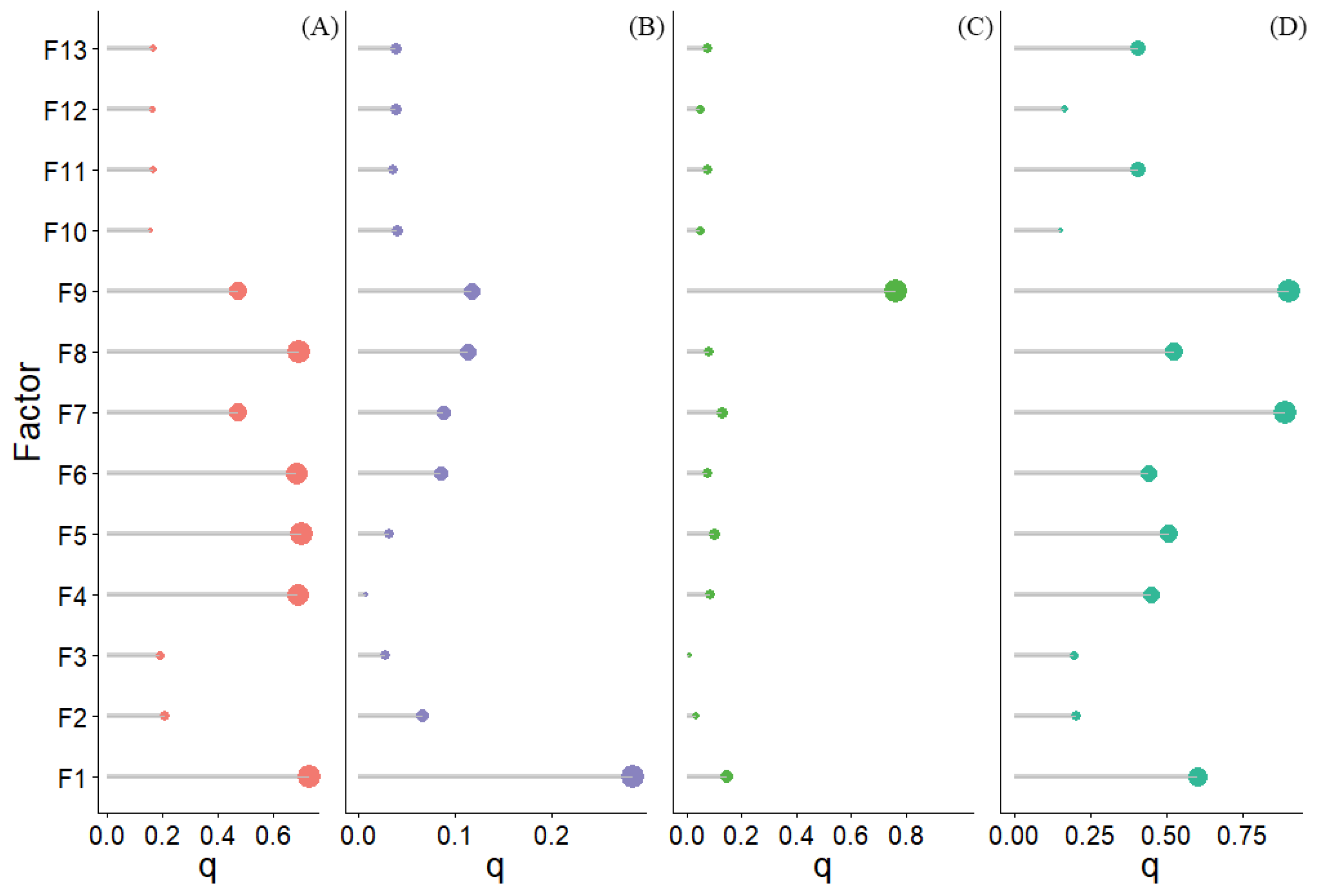
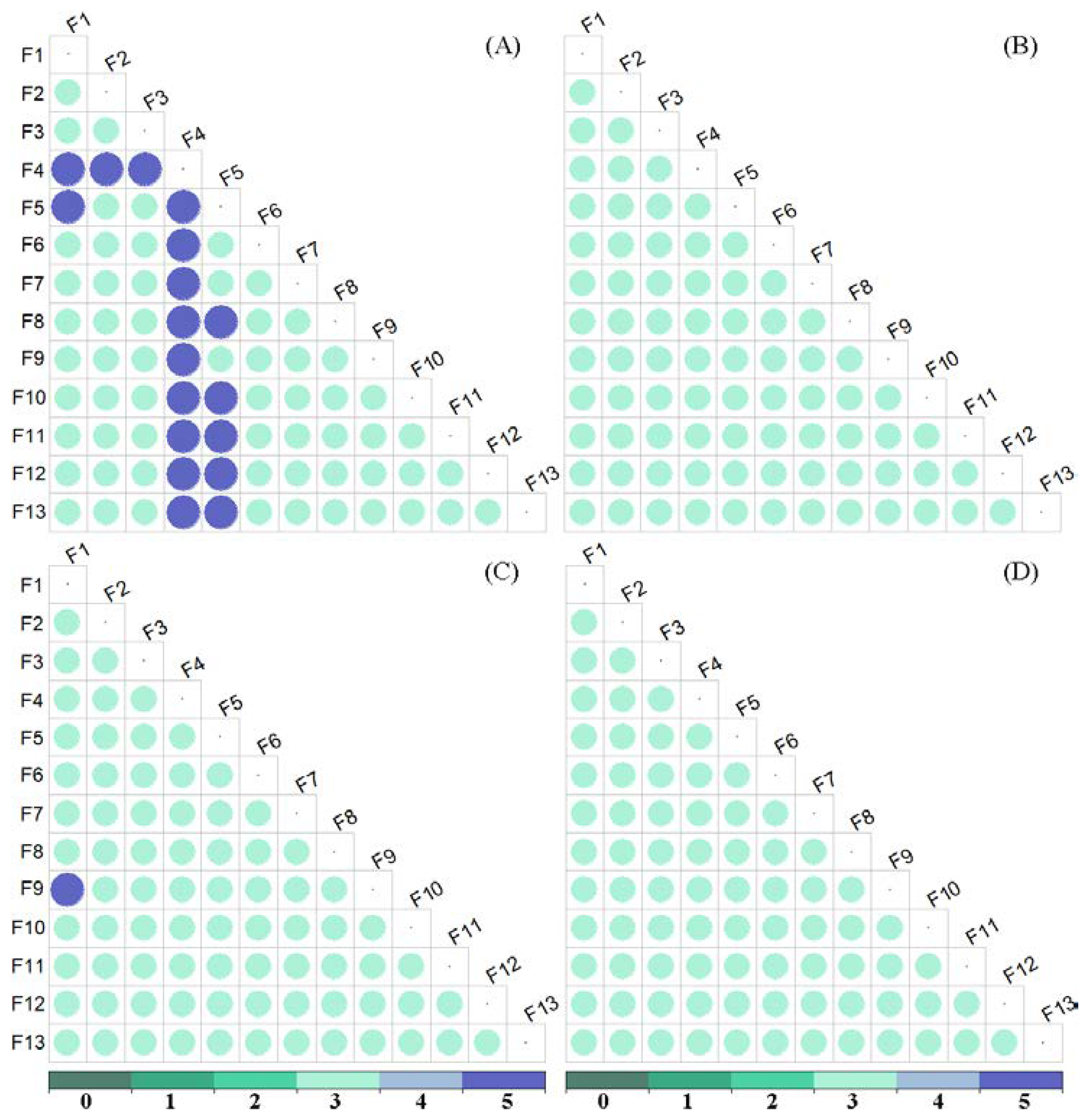
3.2. Potential Driving Factors of Mariculture Expansion
4. Discussion
4.1. Effectiveness of the Proposed Method
4.2. Pattern of Mariculture Dynamics
4.3. Main Drivers of Mariculture Dynamics
4.4. Management Implications and Limitations
5. Conclusions
Author Contributions
Funding
Institutional Review Board Statement
Informed Consent Statement
Data Availability Statement
Acknowledgments
Conflicts of Interest
Appendix A


Appendix B

| Land Cover Type | Distribution Area | Image Interpretation Key and Remote Sensing Image Feature | |||
|---|---|---|---|---|---|
| Landsat 8 OLI | Sentinel-2 | ||||
| Pond | Distributed in the gulf coastal zone |  | Regular shape, blue or blue-black colour |  | Regular shape, green or dark green |
| Mudflat | Distributed in tidal flats along the coast extending into the sea |  | With linear borders and is blue-white in colour |  | With linear borders, the colour is earthen yellow |
| Raft | It’s found all over the bay |  | Regular shape, dark blue colour |  | Regular shape, black colour |
| Cage | It’s found all over the bay |  | Rectangular shape, reddish in colour. |  | Rectangular shape, dark red in colour |
| Seawater | It’s found all over the bay |  | The colour is blue |  | The Colour is green |
| Vegetation cover | Distributed in islands and estuaries |  | The colour is red |  | The colour is bright red |
| Salt pan | Mainly adjacent to the pond |  | Rectangular shape and dark red in colour |  | Rectangular shape and dark red in colour |
| Construction land | Distributed in terrestrial parts of estuaries |  | No obvious texture, colour mixed grey and reddish |  | No obvious texture, colour mixed grey and red |
| Senor | Band Number and Name | Central Wavelength (μm) | Resolution (m) |
|---|---|---|---|
| Landsat8 OLI | Band1 Coastal | 0.443 | 30 |
| Band2 Blue | 0.483 | 30 | |
| Band3 Green | 0.563 | 30 | |
| Band4 Red | 0.655 | 30 | |
| Band5 NIR | 0.865 | 30 | |
| Band7 SWIR 2 | 2.200 | 30 | |
| Sentinel-2 MSI | Band2 Blue | 0.490 | 10 |
| Band3 Green | 0.560 | 10 | |
| Band4 Red | 0.665 | 10 | |
| Band8 NIR | 0.842 | 10 |
| Year | Overall Accuracy | Producer’s Accuracy | User’s Accuracy | Kappa Accuracy |
|---|---|---|---|---|
| 2013 | 0.924 | 0.904 | 0.932 | 0.901 |
| 2014 | 0.951 | 0.934 | 0.967 | 0.934 |
| 2015 | 0.871 | 0.850 | 0.901 | 0.832 |
| 2016 | 0.926 | 0.914 | 0.930 | 0.902 |
| 2017 | 0.923 | 0.912 | 0.910 | 0.9 |
| 2018 | 0.945 | 0.926 | 0.941 | 0.928 |
| 2019 | 0.926 | 0.858 | 0.939 | 0.903 |
| 2020 | 0.940 | 0.923 | 0.918 | 0.922 |
| 2021 | 0.929 | 0.927 | 0.899 | 0.907 |
| Land Cover Type | 2013 | 2018 | 2021 | |||
|---|---|---|---|---|---|---|
| Producer’s Accuracy | User’s Accuracy | Producer’s Accuracy | User’s Accuracy | Producer’s Accuracy | User’s Accuracy | |
| Sea Water | 0.817 | 0.915 | 0.696 | 0.946 | 0.845 | 0.863 |
| Raft | 0.906 | 0.886 | 0.974 | 0.886 | 0.949 | 0.886 |
| Cage | 0.793 | 0.913 | 0.793 | 0.982 | 0.793 | 0.895 |
| Pond | 0.967 | 0.958 | 0.974 | 0.959 | 0.945 | 0.939 |
| Mudflat | 0.923 | 0.860 | 0.986 | 0.956 | 0.918 | 0.981 |
| Vegetation Cover | 1 | 0.977 | 1 | 1 | 1 | 1 |
| Construction Land | 0.875 | 1 | 1 | 0.833 | 1 | 0.667 |
| Salt Pans | 0.951 | 0.947 | 0.983 | 0.963 | 0.963 | 0.959 |
| Land Cover Type | The Number of Ground Truth Points | Accuracy | |
|---|---|---|---|
| Landsat 8 OLI | Sentinel-2 | ||
| Pond | 150 | 0.853 | 0.866 |
| Mudflat | 80 | 0.801 | 0.838 |
| Raft | 260 | 0.835 | 0.840 |
| Cage | 100 | 0.813 | 0.833 |
| Seawater | 80 | 0.805 | 0.812 |
| Vegetation cover | 20 | 0.871 | 0.885 |
| Salt pan | 60 | 0.822 | 0.850 |
| Construction land | 50 | 0.862 | 0.878 |
| Factors\Name | RM | CM | PM | MM | ||||
|---|---|---|---|---|---|---|---|---|
| q | p | q | p | q | p | q | p | |
| F1 | 0.731 | 0.000 | 0.28 | 0.000 | 0.146 | 0.000 | 0.601 | 0.000 |
| F2 | 0.207 | 0.000 | 0.284 | 0.000 | 0.035 | 0.000 | 0.205 | 0.000 |
| F3 | 0.188 | 0.000 | 0.066 | 0.000 | 0.013 | 0.000 | 0.195 | 0.000 |
| F4 | 0.690 | 0.000 | 0.027 | 0.000 | 0.087 | 0.000 | 0.447 | 0.000 |
| F5 | 0.705 | 0.000 | 0.007 | 0.048 | 0.098 | 0.000 | 0.509 | 0.000 |
| F6 | 0.687 | 0.000 | 0.032 | 0.000 | 0.076 | 0.000 | 0.442 | 0.000 |
| F7 | 0.476 | 0.000 | 0.085 | 0.000 | 0.127 | 0.000 | 0.890 | 0.000 |
| F8 | 0.693 | 0.000 | 0.087 | 0.000 | 0.081 | 0.000 | 0.526 | 0.000 |
| F9 | 0.476 | 0.000 | 0.113 | 0.000 | 0.764 | 0.000 | 0.901 | 0.000 |
| F10 | 0.155 | 0.000 | 0.116 | 0.000 | 0.047 | 0.000 | 0.151 | 0.000 |
| F11 | 0.164 | 0.000 | 0.039 | 0.038 | 0.076 | 0.000 | 0.407 | 0.000 |
| F12 | 0.160 | 0.000 | 0.036 | 0.111 | 0.048 | 0.000 | 0.164 | 0.000 |
| F13 | 0.165 | 0.000 | 0.038 | 0.050 | 0.077 | 0.000 | 0.407 | 0.000 |
References
- United Nations General Assembly. Transforming Our World: The 2030 Agenda for Sustainable Development; United Nations General Assembly: New York, NY, USA, 2015. [Google Scholar]
- FAO. World Food and Agriculture—Statistical Yearbook 2021; FAO: Rome, Italy, 2021. [Google Scholar] [CrossRef]
- Zhang, R.; Pei, J.; Zhang, R.; Wang, S.; Zeng, W.; Huang, D.; Wang, Y.; Zhang, Y.; Wang, Y.; Yu, K. Occurrence and distribution of antibiotics in mariculture farms, estuaries and the coast of the Beibu Gulf, China. Bioconcentration and diet safety of seafood. Ecotoxicol. Environ. Saf. 2018, 154, 27–35. [Google Scholar] [CrossRef] [PubMed]
- FAO. The State of World Fisheries and Aquaculture 2020 (SOFIA); FAO: Rome, Italy, 2020. [Google Scholar]
- Alexander, R.B.; Smith, R.A.; Schwarz, G.E. Effect of stream channel size on the delivery of nitrogen to the Gulf of Mexico. Nature 2000, 403, 758–761. [Google Scholar] [CrossRef]
- Ps, P.; Aithal, B.H. Building footprint extraction from very high-resolution satellite images using deep learning. J. Spat. Sci. 2022, 10, 1–17. [Google Scholar] [CrossRef]
- Voutsinou-Taliadouri, F. Metal pollution in the Saronikos Gulf. Mar. Pollut. Bull. 1981, 12, 163–168. [Google Scholar] [CrossRef]
- Ameen, F.; Al-Homaidan, A.A.; Almahasheer, H.; Dawoud, T.; Alwakeel, S.; AlMaarofi, S. Biomonitoring coastal pollution on the Arabian Gulf and the Gulf of Aden using macroalgae. A review. Mar. Pollut. Bull. 2022, 175, 113156. [Google Scholar] [CrossRef] [PubMed]
- DeLaune, R.D.; Wright, A.L. Projected Impact of Deepwater Horizon Oil Spill on U.S. Gulf Coast Wetlands. Soil Sci. Soc. Am. J. 2011, 75, 1602–1612. [Google Scholar] [CrossRef]
- Wang, X.; Zhang, Z.; Dai, H. Detection of remote sensing targets with angles via modified CenterNet. Comput. Electr. Eng. 2022, 100, 107979. [Google Scholar] [CrossRef]
- Sahour, H.; Kemink, K.M.; O’Connell, J. Integrating SAR and Optical Remote Sensing for Conservation-Targeted Wetlands Mapping. Remote Sens. 2022, 14, 159. [Google Scholar] [CrossRef]
- Cui, B.; Fei, D.; Shao, G.; Lu, Y.; Chu, J. Extracting Raft Aquaculture Areas from Remote Sensing Images via an Improved U-Net with a PSE Structure. Remote Sens. 2019, 11, 2053. [Google Scholar] [CrossRef]
- Wang, Z.; Yang, X.; Liu, Y.; Lu, C. Extraction of coastal raft cultivation area with heterogeneous water background by thresholding object-based visually salient NDVI from high spatial resolution imagery. Remote Sens. Lett. 2018, 9, 839–846. [Google Scholar] [CrossRef]
- Hu, Y.; Fan, J.; Wang, J. Target recognition of floating raft aquaculture in SAR image based on statistical region merging. In Proceedings of the 2017 Seventh International Conference on Information Science and Technology (ICIST), Da Nang, Vietnam, 16–19 April 2017; pp. 429–432. [Google Scholar]
- Duan, Y.; Li, X.; Zhang, L.; Chen, D.; Liu, S.; Ji, H. Mapping national-scale aquaculture ponds based on the Google Earth Engine in the Chinese coastal zone. Aquaculture 2020, 520, 734666. [Google Scholar] [CrossRef]
- Sun, Z.; Luo, J.; Yang, J.; Yu, Q.; Zhang, L.; Xue, K.; Lu, L. Nation-Scale Mapping of Coastal Aquaculture Ponds with Sentinel-1 SAR Data Using Google Earth Engine. Remote Sens. 2020, 12, 3086. [Google Scholar] [CrossRef]
- Wu, J.; Del Valle, T.M.; Ruckelshaus, M.; He, G.; Fu, Y.; Deng, J.; Liu, J.; Yang, W. Dramatic mariculture expansion and associated driving factors in Southeastern China. Landsc. Urban Plan. 2021, 214, 104190. [Google Scholar] [CrossRef]
- Jia, M.; Wang, Z.; Mao, D.; Ren, C.; Wang, C.; Wang, Y. Rapid, robust, and automated mapping of tidal flats in China using time series Sentinel-2 images and Google Earth Engine. Remote Sens. Environ. 2021, 255, 112285. [Google Scholar] [CrossRef]
- Zhang, K.; Dong, X.; Liu, Z.; Gao, W.; Hu, Z.; Wu, G. Mapping Tidal Flats with Landsat 8 Images and Google Earth Engine. A Case Study of the China’s Eastern Coastal Zone circa 2015. Remote Sens. 2019, 11, 924. [Google Scholar] [CrossRef]
- Li, Q.; Jin, R.; Ye, Z.; Gu, J.; Dan, L.; He, J.; Christakos, G.; Agusti, S.; Duarte, C.M.; Wu, J. Mapping seagrass meadows in coastal China using GEE. Geocarto Int. 2022, 37, 1–16. [Google Scholar] [CrossRef]
- Akhoondzadeh, M. Advances in Seismo-LAI anomalies detection within Google Earth Engine (GEE) cloud platform. Adv. Space Res. 2022, 69, 4351–4357. [Google Scholar] [CrossRef]
- Yu, Z.; Chang, R.; Chen, Z. Automatic Detection Method for Loess Landslides Based on GEE and an Improved YOLOX Algorithm. Remote Sens. 2022, 14, 4599. [Google Scholar] [CrossRef]
- Gumma, M.K.; Thenkabail, P.S.; Panjala, P.; Teluguntla, P.; Yamano, T.; Mohammed, I. Multiple agricultural cropland products of South Asia developed using Landsat-8 30 m and MODIS 250 m data using machine learning on the Google Earth Engine (GEE) cloud and spectral matching techniques (SMTs) in support of food and water security. GIScience Remote Sens. 2022, 59, 1048–1077. [Google Scholar] [CrossRef]
- Tamiminia, H.; Salehi, B.; Mahdianpari, M.; Quackenbush, L.; Adeli, S.; Brisco, B. Google Earth Engine for geo-big data applications. A meta-analysis and systematic review. ISPRS J. Photogramm. Remote Sens. 2020, 164, 152–170. [Google Scholar] [CrossRef]
- Waleed, M.; Mubeen, M.; Ahmad, A.; Habib-ur-Rahman, M.; Amin, A.; Farid, H.U.; Hussain, S.; Ali, M.; Qaisrani, S.A.; Nasim, W.; et al. Evaluating the efficiency of coarser to finer resolution multispectral satellites in mapping paddy rice fields using GEE implementation. Sci. Rep. 2022, 12, 13210. [Google Scholar] [CrossRef] [PubMed]
- Sha, T.; Yao, X.; Wang, Y.; Tian, Z. A Quick Detection of Lake Area Changes and Hazard Assessment in the Qinghai–Tibet Plateau Based on GEE. A Case Study of Tuosu Lake. Front. Earth Sci. 2022, 10, 103. [Google Scholar] [CrossRef]
- Cheng, B.; Liang, C.; Liu, X.; Liu, Y.; Ma, X.; Wang, G. Research on a novel extraction method using Deep Learning based on GF-2 images for aquaculture areas. Int. J. Remote Sens. 2020, 41, 3575–3591. [Google Scholar] [CrossRef]
- Kang, J.; Sui, L.; Yang, X.; Liu, Y.; Wang, Z.; Wang, J.; Yang, F.; Liu, B.; Ma, Y. Sea Surface-Visible Aquaculture Spatial-Temporal Distribution Remote Sensing. A Case Study in Liaoning Province, China from 2000 to 2018. Sustainability 2019, 11, 7186. [Google Scholar] [CrossRef]
- Zhang, Y.; Wang, C.; Chen, J.; Wang, F. Shape-Constrained Method of Remote Sensing Monitoring of Marine Raft Aquaculture Areas on Multitemporal Synthetic Sentinel-1 Imagery. Remote Sens. 2022, 14, 1249. [Google Scholar] [CrossRef]
- Duan, Y.; Li, X.; Zhang, L.; Liu, W.; Liu, S.; Chen, D.; Ji, H. Detecting spatiotemporal changes of large-scale aquaculture ponds regions over 1988–2018 in Jiangsu Province, China using Google Earth Engine. Ocean Coast. Manag. 2020, 188, 105144. [Google Scholar] [CrossRef]
- Xu, Y.; Hu, Z.; Zhang, Y.; Wang, J.; Yin, Y.; Wu, G. Mapping Aquaculture Areas with Multi-Source Spectral and Texture Features. A Case Study in the Pearl River Basin (Guangdong), China. Remote Sens. 2021, 13, 4320. [Google Scholar] [CrossRef]
- Cheng, M.; Jiao, X.; Shi, L.; Penuelas, J.; Kumar, L.; Nie, C.; Wu, T.; Liu, K.; Wu, W.; Jin, X. High-resolution crop yield and water productivity dataset generated using random forest and remote sensing. Sci. Data 2022, 9, 641. [Google Scholar] [CrossRef]
- Loozen, Y.; Rebel, K.T.; de Jong, S.M.; Lu, M.; Ollinger, S.V.; Wassen, M.J.; Karssenberg, D. Mapping canopy nitrogen in European forests using remote sensing and environmental variables with the random forests method. Remote Sens. Environ. 2020, 247, 111933. [Google Scholar] [CrossRef]
- Wang, Q.; Zhao, L.; Wang, M.; Wu, J.; Zhou, W.; Zhang, Q.; Deng, M. A Random Forest Model for Drought. Monitoring and Validation for Grassland Drought Based on Multi-Source Remote Sensing Data. Remote Sens. 2022, 14, 4981. [Google Scholar] [CrossRef]
- Ghorbanian, A.; Zaghian, S.; Asiyabi, R.M.; Amani, M.; Mohammadzadeh, A.; Jamali, S. Mangrove Ecosystem Mapping Using Sentinel-1 and Sentinel-2 Satellite Images and Random Forest Algorithm in Google Earth Engine. Remote Sens. 2021, 13, 2565. [Google Scholar] [CrossRef]
- Matarira, D.; Mutanga, O.; Naidu, M. Google Earth Engine for Informal Settlement Mapping. A Random Forest Classification Using Spectral and Textural Information. Remote Sens. 2022, 14, 5130. [Google Scholar] [CrossRef]
- Phan, T.N.; Kuch, V.; Lehnert, L.W. Land Cover Classification using Google Earth Engine and Random Forest Classifier—The Role of Image Composition. Remote Sens. 2020, 12, 2411. [Google Scholar] [CrossRef]
- Ying, Z.; Wu, J.; Del Valle, T.M.; Yang, W. Spatiotemporal dynamics of coastal aquaculture and driving force analysis in Southeastern China. Ecosyst. Health Sustain. 2020, 6, 1851145. [Google Scholar] [CrossRef]
- Giri, S.; Daw, T.M.; Hazra, S.; Troell, M.; Samanta, S.; Basu, O.; Marcinko, C.L.J.; Chanda, A. Economic incentives drive the conversion of agriculture to aquaculture in the Indian Sundarbans: Livelihood and environmental implications of different aquaculture types. AMBIO 2022, 51, 1963–1977. [Google Scholar] [CrossRef]
- Wang, J.-F.; Zhang, T.-L.; Fu, B.-J. A measure of spatial stratified heterogeneity. Ecol. Indic. 2016, 67, 250–256. [Google Scholar] [CrossRef]
- Wang, J.-F.; Li, X.-H.; Christakos, G.; Liao, Y.-L.; Zhang, T.; Gu, X.; Zheng, X.-Y. Geographical Detectors-Based Health Risk Assessment and its Application in the Neural Tube Defects Study of the Heshun Region, China. Int. J. Geogr. Inf. Sci. 2010, 24, 107–127. [Google Scholar] [CrossRef]
- Qiao, Y.; Wang, X.; Han, Z.; Tian, M.; Wang, Q.; Wu, H.; Liu, F. Geodetector based identification of influencing factors on spatial distribution patterns of heavy metals in soil. A case in the upper reaches of the Yangtze River, China. Appl. Geochem. 2022, 146, 105459. [Google Scholar] [CrossRef]
- Zhao, R.; Zhan, L.; Yao, M.; Yang, L. A geographically weighted regression model augmented by Geodetector analysis and principal component analysis for the spatial distribution of PM2.5. Sustain. Cities Soc. 2020, 56, 102106. [Google Scholar] [CrossRef]
- Yang, Y.; Yang, X.; He, M.; Christakos, G. Beyond mere pollution source identification. Determination of land covers emitting soil heavy metals by combining PCA/APCS, GeoDetector and GIS analysis. CATENA 2020, 185, 104297. [Google Scholar] [CrossRef]
- Zhou, X.; Wen, H.; Zhang, Y.; Xu, J.; Zhang, W. Landslide susceptibility mapping using hybrid random forest with GeoDetector and RFE for factor optimization. Geosci. Front. 2021, 12, 101211. [Google Scholar] [CrossRef]
- Gu, J.; Liang, L.; Song, H.; Kong, Y.; Ma, R.; Hou, Y.; Zhao, J.; Liu, J.; He, N.; Zhang, Y. A method for hand-foot-mouth disease prediction using GeoDetector and LSTM model in Guangxi, China. Sci. Rep. 2019, 9, 17928. [Google Scholar] [CrossRef] [PubMed]
- Su, Y.; Li, T.; Cheng, S.; Wang, X. Spatial distribution exploration and driving factor identification for soil salinisation based on geodetector models in coastal area. Ecol. Eng. 2020, 156, 105961. [Google Scholar] [CrossRef]
- Yuanxin, Y. Lethal effects of suspended sediment on juvenile and young Acanthopagrus latus in Bachimen waters of Dongshan. J. Fish. Res. 2021, 43, 571–577. [Google Scholar]
- Xiang, L. Principal Component Linear Regression Analysis on Chlorophyll-a and Environmental Factors in Aquiculture Area, Zhao’an Bay. Environ. Impact Assess. 2018, 40, 88–96. [Google Scholar]
- Yingyu, X.; Jiao, L.; Yongqing, L.; Miaofeng, Y. Distributional and risk assessment of Hg and As in the culture-shellish from southern coastal areas of Fujian Province. Environ. Chem. 2017, 36, 1009–1016. [Google Scholar]
- Shuoliang, Z.; Jingshan, R.; Yingyu, X.; Lifeng, W.; Shenghua, Z.; Miaofeng, Y.; Ying, Y.; Yufeng, C. Study on assessment and categorization for the eco—Environmental quality of shellfish—Culture regions in Zhao’an Bay, Fujian province. J. Fujian Fish. 2012, 34, 268–276. [Google Scholar]
- Ministry of Natural Resources (PRC). Bulletin on China’s Marine Ecological Environment in 2021. 2022. Available online: http://news.mnr.gov.cn/dt/hy/202206/t20220606_2738442.html (accessed on 6 June 2022).
- Arcgis Pro. 2019. Available online: https://www.esri.com/zh-cn/arcgis/products/arcgis-pro/overview (accessed on 3 May 2019).
- Ruff, E.O.; Gentry, R.R.; Clavelle, T.; Thomas, L.R.; Lester, S.E. Governance and mariculture in the Caribbean. Mar. Policy 2019, 107, 103565. [Google Scholar] [CrossRef]
- Sarker, S.; Akter, M.; Rahman, M.S.; Islam, M.M.; Hasan, O.; Kabir, M.A.; Rahman, M.M. Spatial prediction of seaweed habitat for mariculture in the coastal area of Bangladesh using a Generalized Additive Model. Algal Res. 2021, 60, 102490. [Google Scholar] [CrossRef]
- Sánchez-Jerez, P.; Babarro, J.M.; Padin, X.A.; Portabales, A.L.; Martinez-Llorens, S.; Ballester-Berman, J.D.; Sara, G.; Mangano, M.C. Cumulative climatic stressors strangles marine aquaculture. Ancillary effects of COVID 19 on Spanish mariculture. Aquaculture 2022, 549, 737749. [Google Scholar] [CrossRef]
- Hillger, D.; Seaman, C.; Liang, C.; Miller, S.; Lindsey, D.; Kopp, T. Suomi NPP VIIRS Imagery evaluation. J. Geophys. Res. Atmos. 2014, 119, 6440–6455. [Google Scholar] [CrossRef]
- Gashaw, T.; Tulu, T.; Argaw, M.; Worqlul, A.W.; Tolessa, T.; Kindu, M. Estimating the impacts of land use/land cover changes on Ecosystem Service Values. The case of the Andassa watershed in the Upper Blue Nile basin of Ethiopia. Ecosyst. Serv. 2018, 31, 219–228. [Google Scholar] [CrossRef]
- Van Asselen, S.; Verburg, P.H.; Vermaat, J.E.; Janse, J.H. Drivers of wetland conversion. A global meta-analysis. PLoS ONE 2013, 8, e81292. [Google Scholar] [CrossRef] [PubMed]
- Wang, L.; Yue, X.; Wang, H.; Ling, K.; Liu, Y.; Wang, J.; Hong, J.; Pen, W.; Song, H. Dynamic Inversion of Inland Aquaculture Water Quality Based on UAVs-WSN Spectral Analysis. Remote Sens. 2020, 12, 402. [Google Scholar] [CrossRef]
- Song, C.; Becagli, S.; Beddows, D.C.S.; Brean, J.; Browse, J.; Dai, Q.; Dall’Osto, M.; Ferracci, V.; Harrison, R.M.; Harris, N.; et al. Understanding Sources and Drivers of Size-Resolved Aerosol in the High Arctic Islands of Svalbard Using a Receptor Model Coupled with Machine Learning. Environ. Sci. Technol. 2022, 56, 11189–11198. [Google Scholar] [CrossRef]
- Chopin, T.; Cooper, J.A.; Reid, G.; Cross, S.; Moore, C. Open-water integrated multi-trophic aquaculture. Environmental biomitigation and economic diversification of fed aquaculture by extractive aquaculture. Rev. Aquac. 2012, 4, 209–220. [Google Scholar] [CrossRef]
- Ren, C.; Wang, Z.; Zhang, Y.; Zhang, B.; Chen, L.; Xi, Y.; Xiao, X.; Doughty, R.B.; Liu, M.; Jia, M.; et al. Rapid expansion of coastal aquaculture ponds in China from Landsat observations during 1984–2016. Int. J. Appl. Earth Obs. Geoinf. 2019, 82, 101902. [Google Scholar] [CrossRef]
- Liu, S. Effect of reclamation activities on wetlands in Estuarine Delta in China. Wetl. Sci. 2013, 11, 297–304. [Google Scholar]
- Chen, H.; Zhao, Y.; Fu, X.; Tang, M.; Guo, M.; Zhang, S.; Zhu, Y.; Qu, L.; Wu, G. Impacts of regional land-use patterns on ecosystem services in the typical agro-pastoral ecotone of northern China. Ecosyst. Health Sustain. 2022, 8, 2110521. [Google Scholar] [CrossRef]
- Foley, J.A.; DeFries, R.; Asner, G.P.; Barford, C.; Bonan, G.; Carpenter, S.R.; Chapin, F.S.; Coe, M.T.; Daily, G.C.; Gibbs, H.K.; et al. Global Consequences of Land Use. Science 2005, 309, 570–574. [Google Scholar] [CrossRef]
- Ministry of Natural Resources (PRC). Bulletin on China’s Marine Ecological Environment in 2019. 2020. Available online: https://www.mee.gov.cn/hjzl/sthjzk/jagb/202006/P020200603371117871012.pdf (accessed on 1 June 2020).
- Zhao’an County People’s Government Office. Notice of Zhao‘an County People’s Government Office on Printing and Distributing the Work Plan of Zhao‘an County on the Control of Fishery Pollution Sources. 2019. Available online: http://www.zhaoan.gov.cn/cms/html/zaxnzz/2019-11-08/1359531076.html (accessed on 8 November 2019).
- Zhao‘an County Bureau of Ocean and Fisheries. A Reply Letter on the Handling of the 4th Session of the 17th County People’s Congress No. 39 Representative’s Proposal. 2020. Available online: http://search.zhangzhou.gov.cn/cms/infopublic/publicInfo.shtml?id=60502325480150004 (accessed on 6 July 2020).
- Sun, X.; Zhang, L.; Lu, S.-Y.; Tan, X.-Y.; Chen, K.-L.; Zhao, S.-Q.; Huang, R.-H. A new model for evaluating sustainable utilization of coastline integrating economic output and ecological impact. A case study of coastal areas in Beibu Gulf, China. J. Clean. Prod. 2020, 271, 122423. [Google Scholar] [CrossRef]
- Zhou, Y.; Li, X.; Liu, Y. Land use change and driving factors in rural China during the period 1995–2015. Land Use Policy 2020, 99, 105048. [Google Scholar] [CrossRef]
- Liu, L. Current situation and countermeasures of sea reclamation in China. Guangzhou Environ. Sci. 2008, 2, 26–30. [Google Scholar]
- Wang, W.; Liu, H.; Li, Y.; Su, J. Development and management of land reclamation in China. Ocean Coast. Manag. 2014, 102, 415–425. [Google Scholar] [CrossRef]
- Wang, X.; Zhou, T.; Ying, Z.; Jing, W.U.; Yang, W. Analyses of water quality and driving forces in Ningde aquaculture area. Acta Ecol. Sin. 2020, 40, 1766–1778. [Google Scholar]
- Ren, C.; Wang, Z.; Zhang, B.; Li, L.; Chen, L.; Song, K.; Jia, M. Remote Monitoring of Expansion of Aquaculture Ponds Along Coastal Region of the Yellow River Delta from 1983 to 2015. Chin. Geogr. Sci. 2018, 28, 430–442. [Google Scholar] [CrossRef]
- MacKinnon, J.; Verkuil, Y.; Murray, N. IUCN Situation Analysis on East and Southeast Asian Intertidal Habitats, with Particular Reference to the Yellow Sea (Including the Bohai Sea); IUCN: Gland, Switzerland, 2012; p. 47. Available online: https://portals.iucn.org/library/efiles/documents/SSC-OP-047.pdf (accessed on 1 January 2012).
- Morgera, E.; Vrancken, P. The ocean, sustainable development and human rights. RECIEL 2022, 31, 333–335. [Google Scholar] [CrossRef]
- Nash, K.L.; van Putten, I.; Alexander, K.A.; Bettiol, S.; Cvitanovic, C.; Farmery, A.K.; Flies, E.J.; Ison, S.; Kelly, R.; Mackay, M.; et al. Oceans and society. Feedbacks between ocean and human health. Rev. Fish Biol. Fish. 2022, 32, 161–187. [Google Scholar] [CrossRef] [PubMed]
- Grant, S.M.; Waller, C.L.; Morley, S.A.; Barnes, D.K.A.; Brasier, M.J.; Double, M.C.; Griffiths, H.J.; Hughes, K.A.; Jackson, J.A.; Waluda, C.M.; et al. Local Drivers of Change in Southern Ocean Ecosystems. Human Activities and Policy Implications. Front. Ecol. Evol. 2021, 9, 624518. [Google Scholar] [CrossRef]
- Pellens, N.; Boelee, E.; Veiga, J.M.; Fleming, L.E.; Blauw, A. Innovative actions in oceans and human health for Europe. Health Promot. Int. 2021, 2021, daab203. [Google Scholar] [CrossRef] [PubMed]
- Hair, C.; Foale, S.; Daniels, N.; Minimulu, P.; Aini, J.; Southgate, P.C. Social and economic challenges to community-based sea cucumber mariculture development in New Ireland Province, Papua New Guinea. Mar. Policy 2020, 117, 103940. [Google Scholar] [CrossRef]
- La Aslan, O.M.; Iba, W.; La Bolu, O.R.; Ingram, B.A.; Gooley, G.J.; de Silva, S.S. Mariculture in SE Sulawesi, Indonesia. Culture practices and the socio economic aspects of the major commodities. Ocean Coast. Manag. 2015, 116, 44–57. [Google Scholar] [CrossRef]
- Rodrigues, J.M.F.; Cardoso, P.J.S.; Monteiro, J.; Lam, R.; Krzhizhanovskaya, V.V.; Lees, M.H.; Dongarra, J.J.; Sloot, P.M.; Lou, Y.; Chen, L.; et al. (Eds.) Research and Implementation of an Aquaculture Monitoring System Based on Flink, MongoDB and Kafka. Computational Science—ICCS 2019; Springer International Publishing: Berlin/Heidelberg, Germany, 2019. [Google Scholar]
- Ubina, N.A.; Cheng, S.-C. A Review of Unmanned System Technologies with Its Application to Aquaculture Farm Monitoring and Management. Drones 2022, 6, 12. [Google Scholar] [CrossRef]
- Alwis, S.D.; Hou, Z.; Zhang, Y.; Na, M.H.; Ofoghi, B.; Sajjanhar, A. A survey on smart farming data, applications and techniques. Comput. Ind. 2022, 138, 103624. [Google Scholar] [CrossRef]
- Kirankumar, P.; Keertana, G.; Sivarao, S.U.A.; Vijaykumar, B.; Shah, S.C. Smart Monitoring and Water Quality Management in Aquaculture using IOT and ML. In Proceedings of the 2021 IEEE International Conference on Intelligent Systems, Smart and Green Technologies (ICISSGT), Visakhapatnam, India, 13–14 November 2021. [Google Scholar] [CrossRef]
- Zhao, S.; Zhang, S.; Liu, J.; Wang, H.; Zhu, J.; Li, D.; Zhao, R. Application of machine learning in intelligent fish aquaculture. A review. Aquaculture 2021, 540, 736724. [Google Scholar] [CrossRef]
- Craig, R.K. Fostering Adaptive Marine Aquaculture through Procedural Innovation in Marine Spatial Planning. Marine Policy 2019, 110, 103555. [Google Scholar] [CrossRef]
- Douvere, F.; Ehler, C.N. New perspectives on sea use management. Initial findings from European experience with marine spatial planning. J. Environ. Manag. 2009, 90, 77–88. [Google Scholar] [CrossRef]
- Yu, J.-K.; Li, Y.-H. Evolution of marine spatial planning policies for mariculture in China. Overview, experience and prospects. Ocean Coast. Manag. 2020, 196, 105293. [Google Scholar] [CrossRef]
- Filgueira, R.; Grant, J.; Strand, Ø. Implementation of marine spatial planning in shellfish aquaculture management. Modeling studies in a Norwegian fjord. Ecol. Appl. 2014, 24, 832–843. [Google Scholar] [CrossRef]
- Roth, E.; Burbridge, P.; Hendrick, V.; Rosenthal, H. Social and economic policy issues relevant to marine aquaculture. J. Appl. Ichthyol. 2001, 17, 194–206. [Google Scholar] [CrossRef]


| Categories | Code | Name | Unit | Detail |
|---|---|---|---|---|
| Mariculture | F1 | area_init | m2 | the initial area of the mariculture, which reflects the potential for the further expansion of a grid |
| F2 | num_type | pcs | the initial number of mariculture types per grid cell | |
| F3 | num_c_type | pcs | the change in the number of mariculture types per grid cell | |
| Geographical factors | F4 | dis_land | m | the centre of the geometric grid closest to the land at the beginning |
| F5 | dis_island | m | the distance from the nearest island | |
| F6 | dis_scell | m | the distance between each grid and its closest neighbours involving the same type of mariculture | |
| F7 | dis_c_scell | m | the change in the distance between each grid and its closest neighbours involving the same type of mariculture | |
| F8 | dis_dcell | m | the distance between each grid cell and its closest neighbours involving a different type of mariculture | |
| F9 | dis_c_dcell | m | the change in distance between each grid cell and its closest neighbours involving a different type of mariculture | |
| Human Factors | F10 | sum_init_light | Nano Watts /cm2/sr | the sum of the night light data for an area > 5 km2 |
| F11 | sum_c_light | the change in the sum of the night-time lighting data | ||
| F12 | ave_init_light | the average of the night light data for an area >5 km2 | ||
| F13 | ave_c_light | the change in the average of night-time lighting data |
| Criteria | Interaction |
|---|---|
| q(×1 ∩ ×2) < min(q(×1), q(×2)) | Weaken—nonlinear |
| min(q(×1),q(×2)) < q(×1 ∩ ×2) < Max(q(×1), q(×2)) | weaken—univariate |
| q(×1 ∩ ×2) > Max(q(×1), q(×2)) | enhance—bivariate |
| q(×1 ∩ ×2) = q(×1) + q(×2) | independent |
| q(×1 ∩ ×2) > q(×1) + q(×2) | enhance—nonlinear |
Disclaimer/Publisher’s Note: The statements, opinions and data contained in all publications are solely those of the individual author(s) and contributor(s) and not of MDPI and/or the editor(s). MDPI and/or the editor(s) disclaim responsibility for any injury to people or property resulting from any ideas, methods, instructions or products referred to in the content. |
© 2023 by the authors. Licensee MDPI, Basel, Switzerland. This article is an open access article distributed under the terms and conditions of the Creative Commons Attribution (CC BY) license (https://creativecommons.org/licenses/by/4.0/).
Share and Cite
Wang, P.; Wang, J.; Liu, X.; Huang, J. A Google Earth Engine-Based Framework to Identify Patterns and Drivers of Mariculture Dynamics in an Intensive Aquaculture Bay in China. Remote Sens. 2023, 15, 763. https://doi.org/10.3390/rs15030763
Wang P, Wang J, Liu X, Huang J. A Google Earth Engine-Based Framework to Identify Patterns and Drivers of Mariculture Dynamics in an Intensive Aquaculture Bay in China. Remote Sensing. 2023; 15(3):763. https://doi.org/10.3390/rs15030763
Chicago/Turabian StyleWang, Peng, Jian Wang, Xiaoxiang Liu, and Jinliang Huang. 2023. "A Google Earth Engine-Based Framework to Identify Patterns and Drivers of Mariculture Dynamics in an Intensive Aquaculture Bay in China" Remote Sensing 15, no. 3: 763. https://doi.org/10.3390/rs15030763
APA StyleWang, P., Wang, J., Liu, X., & Huang, J. (2023). A Google Earth Engine-Based Framework to Identify Patterns and Drivers of Mariculture Dynamics in an Intensive Aquaculture Bay in China. Remote Sensing, 15(3), 763. https://doi.org/10.3390/rs15030763