Article

Assessing Temporal Trade-Offs of Ecosystem Services by Production Possibility Frontiers

State Key Laboratory of Urban and Regional Ecology, Research Center for Eco-Environmental Sciences, Chinese Academy of Sciences, Beijing 100085, China
*
Author to whom correspondence should be addressed.
Remote Sens. 2023, 15(3), 749; https://doi.org/10.3390/rs15030749
Submission received: 15 December 2022 / Revised: 16 January 2023 / Accepted: 25 January 2023 / Published: 28 January 2023
(This article belongs to the Section Ecological Remote Sensing)

Abstract

:
Ecosystems provide multiple valuable services that play an essential role in preventing meteorological risks, combating sandy land expansion, and ensuring sustainable development in the West Liao River Basin. The trade-off among ecosystem services (ES) is inevitable because of biophysical constraints and societal preferences. The production possibility frontier (PPF) is increasingly deemed an appropriate tool for representing trade-off relationships among ES. In this study, we developed a feasible approach for estimating PPF, which includes three steps. First, the annual water yield model, the sediment delivery ratio model, the carbon storage and sequestration model, and the habitat quality model of InVEST models were used to quantify temporal changes in four key ES, including water retention, soil conservation, carbon sequestration, and habitat improvement, in five-year periods from 1990 to 2020. Second, after the standardization of ES quantities, the functional forms of PPF curves for six pairs of ES trade-offs were derived by adopting a two-term exponential function of the curve fitting tool in MATLAB. Third, the trade-off intensity for each ES pair was defined and calculated based on the distance from the mean point to the PPF curve. Compared to the existing approaches, our approach has the advantage of fitting functional forms of PPF curves, handling both positive and negative values of ES, and calculating trade-off intensities. This study has three implications. First, showing the trade-offs between ES by PPF is helpful for providing knowledge on the existence of turning points and a complex relationship between certain ES pairs, thus avoiding unintended and large-scale shifts in the provision of ES. Second, PPF curves are a useful tool for visualizing the nature of ES relationships and the changes in trade-off intensity, thus supporting decision-makers to identify optimal solutions and make land use planning that can increase the overall efficiency over multiple ES. Third, socioeconomic components should be integrated into the assessment of ES trade-offs in order to understand the influences of societal choices on and examine stakeholders’ preferences regarding efficient ES combinations.

1. Introduction

Ecosystem services (ES) are the direct or indirect benefits that people derive from the ecological components, processes, and functions of functioning ecosystems [1,2]. The concept of ES has been popularly used in recent decades to enable the understanding of ecosystem potentials for the sustainable supply of various services, such as provisioning, regulating, cultural, and supporting ES, and the incorporating of ES into concerned key themes, such as biodiversity conservation, economic valuation of natural capital, and landscape planning, etc. [3,4].
The simultaneous supply of multiple ES is usually restricted by biophysical constraints to a certain extent, making trade-offs inevitable [5]. The ES trade-offs refer to the situation that the increase in one ES leads to a decrease in the other ES and vice versa, which is prominent among different ES types and occurs at both a spatial and temporal scale [6,7,8]. Trade-offs between ES can be attracted to two types of mechanisms: direct interactions between ES [9] or indirect interactions via the effects of common drivers influencing ES [10], such as the ecological processes underlying ES [11]. Since humankind nowadays is confronted with severe challenges, including climate change, population growth, and resource exhaustion [12], “trade-off thinking” contributes to examining the existing shortcomings, improving management approaches, and making the most reasonable choices under limited conditions [13]. It is challenging to analyze ES trade-offs because of the potential non-linearity of their temporal and spatial variations [14]. The research trend indicates that current studies deal more with static spatial correlations among ES but consider temporal dynamics of ES trade-offs less; therefore, insufficient studies were carried out to capture the comprehensive understanding of ES interactions at the river basin scale [4].
Various methodological approaches exist to assess ES trade-offs, including statistical analysis [15], spatial mapping [16], model simulation [17], and economic valuation [18]. In the recent literature, the application of production possibility frontiers (PPF) to characterize ES trade-offs has drawn increasing attention [19,20,21]. PPF, also known as efficiency frontiers, is a basic concept in welfare economics and production theory that represents the combination of the largest amount of various commodities produced in an economy with given resources and technology conditions [22]. In analogy, PPF has been developed to describe combinations of multiple ES supplies and can be accommodated within a landscape given its ecological characteristics and human inputs, indicating the optimal balance between two conflicting ES [23,24]. PPF is determined by biophysical and socio-economic constraints and thus varies with geographical locations, climatic characteristics, physical disturbance (e.g., fire, extreme events), and human interference (e.g., land use change, management practices) [8,25,26]. However, a general operational approach for estimating PPFs, as well as their functional forms, is still missing [19,24,27,28]. Furthermore, an appropriate index that represents the intensity of trade-offs should be explored [29].
The West Liao River Basin (WLRB) is a sub-watershed of the Liao River Basin that is one of seven large river basins in China. The WLRB is a typical agro-pastoral transitional zone located in the semi-arid region, where the long-term tendency of drought and intensive crop production and grazing has resulted in the drying up of the West Liao River, along with water decline in the major lakes and reservoirs, and groundwater depletion [30,31]. The issues of water scarcity, soil erosion, and climate change exacerbated grassland degradation and desertification, making ecosystems in the WLRB vulnerable [32,33]. The ES and their relationships play an important role in preventing meteorological risk, maintaining stable agricultural production, combating sandy land expansion, and ensuring sustainable development in this region. However, studies that investigate ES and its trade-offs have still not been found in this important region.
Therefore, the main purpose of this paper was to develop an operational approach for estimating functional forms of PPFs and calculating trade-off intensities. Taking the WLRB as a case study, we apply this approach to the temporal variations of ES interactions at the river basin scale. Because of the great significance of water, soil, air, and biodiversity in adapting to water scarcity, soil erosion, climate change, and habitat degradation in the WLRB region, respectively, we focused on four fundamental ES, including water retention (WR), soil conservation (SC), carbon sequestration (CS), and habitat improvement (HI). Thus, the interactions of six pairs of ES have been considered for trade-off analysis, WR-SC, WR-CS, WR-HI, SC-CS, SC-HI, and CS-HI.

2. Materials and Methods

2.1. Study Area

The WLRB is located in the southeastern corner of Inner Mongolia in Northeast China, adjacent to Hebei, Liaoning, and Jilin (Figure 1a). Its geographic position ranges between 116°–125°E and 41°–46°N, covering an area of 126,528 km2. The climate is characterized by the temperate continental monsoon type with an annual mean air temperature of 5.0℃ to 6.5℃ and an annual average precipitation of about 376 mm, which is concentrated in July and August [34]. The overall topography decreases from west to east and relates to the main land cover types (Figure 1b). Forests are fragmentarily distributed on the western mountains, grasslands and sparse vegetation are distributed in the mountain-plain transitional region, the eastern plain is mainly covered by dry farmlands and paddy fields, the central bare area is the Horqin Sandy Land, and the major built-up areas are Tongliao City and Chifeng City (Figure 1c).

2.2. Data Sources and Pre-Processing

Multi-source spatial data were collected, among which data on land use/land cover, precipitation, and evapotranspiration included temporal variations for the years 1990, 1995, 2000, 2005, 2010, 2015, and 2020 (Table 1). In order to run InVEST models, the usually different original projections and resolutions of these spatial data were standardized by re-projecting and resampling using ArcGIS Desktop 10.6 [35]. The resampling was performed using the built-in CUBIC technique of ArcGIS software, which calculates the value of each pixel by fitting a smooth curve based on the surrounding 16 pixels, thus producing the smoothest image. Since InVEST models are based on land use/land cover data, they are resampled to the spatial resolution of 30m × 30m in order to maintain the original data quality.

2.3. Quantifying ES and Temporal Changes

Considering the most important ecological indicators of water, soil, air, and biology, four ES were selected for analysis, namely water retention (WR), soil conservation (SC), carbon sequestration (CS), and habitat improvement (HI). Correspondingly, we used the annual water yield model, the sediment delivery ratio model, the carbon storage and sequestration model, and the habitat quality model of InVEST 3.12 to quantify these four ES [46].
The annual water yield model estimates the relative contributions of water from different parts of a landscape, offering insight into how changes in land use/land cover patterns affect the annual surface of water yield. The sediment delivery ratio model spatially and explicitly computes the amount of annual soil loss from each pixel at the spatial resolution of the input digital elevation model raster, then computes the sediment delivery ratio, which is the proportion of soil loss that actually reaches the stream. The carbon storage and sequestration model aggregates the amount of carbon stored in four carbon pools according to land use/land cover maps and classifications: aboveground biomass, belowground biomass, soil, and dead organic matter. The habitat quality model combines information on land use/land cover and threats to biodiversity in order to produce habitat quality maps, which represent the relative extent and degradation of different habitat types in a region (Table 2) [47].
The model performances generated 28 datasets (four ES, i.e., water yield, soil deposition, carbon storage, habitat quality, in seven years, i.e., 1990, 1995, 2000, 2005, 2010, 2015, and 2020) for each pixel out of a total of 140,723,294 pixels in the WLRB. The positive and negative changes in ES between the years can be interpreted as ecological processes (Table 3). Thus, 28 datasets are calculated into 24 new datasets that represent the changes in the four ES (WR, SC, CS, and HI) in six periods (1990–1995, 1995–2000, 2000–2005, 2005–2010, 2010–2015, and 2015–2020) by using the Raster Calculator tool in the ArcGIS Desktop 10.6 [35].

2.4. Estimating PPF Curves

In order to make multiple ES comparable, the value of ES should be nondimensionalized and standardized. The arc-tangent function was selected for standardization because it is a monotone-increasing function that converts the original values into values between −1 and 1 regardless of negative or positive values. The standardization was processed by the Raster Calculator tool in ArcGIS Desktop 10.6 [35]. Owing to the limits of both hardware and software, not all 140,723,294 pixels in the WLRB could be taken into account; a sampling of 50,000 pixels was needed for the use of the Create Random Points tool in ArcGIS Desktop 10.6 [35]. Thus, we obtained 50,000 pixels for further analysis, each of which included 24 values (4 ES × 6 periods).
The pairwise comparison between ES was conducted, generating six pairs, including WR-SC, WR-CS, WR-HI, SC-CS, SC-HI, and CS-HI, in six periods, respectively. Taking the pair of WR-SC in the period 1990–1995 as an example, the values of WR and SC in 50,000 pixels were used to build two-dimension scatter points with the value of WR as the x-axis and the value of SC as the y-axis. We used the boundary function in MATLAB R2021b [48] to identify the boundary points, which were distributed in four quadrants. We then selected the boundary points in the first quadrant to estimate PPF because the other points were assumed to be enveloped by the frontier emerging from these boundary points. We adopted the two-term exponential function of the Curve Fitting tool in MATLAB R2021b [48] to fit the PPF curves:
y = k 1 + k 2 × e x k 0 k 4 + k 3 × e x k 0 k 5 ,
where k0, k1, k2, k3, k4, and k5 are coefficients to be fitted, and x and y are variables that denote the value of two ES.

2.5. Calculating Trade-Off Intensity

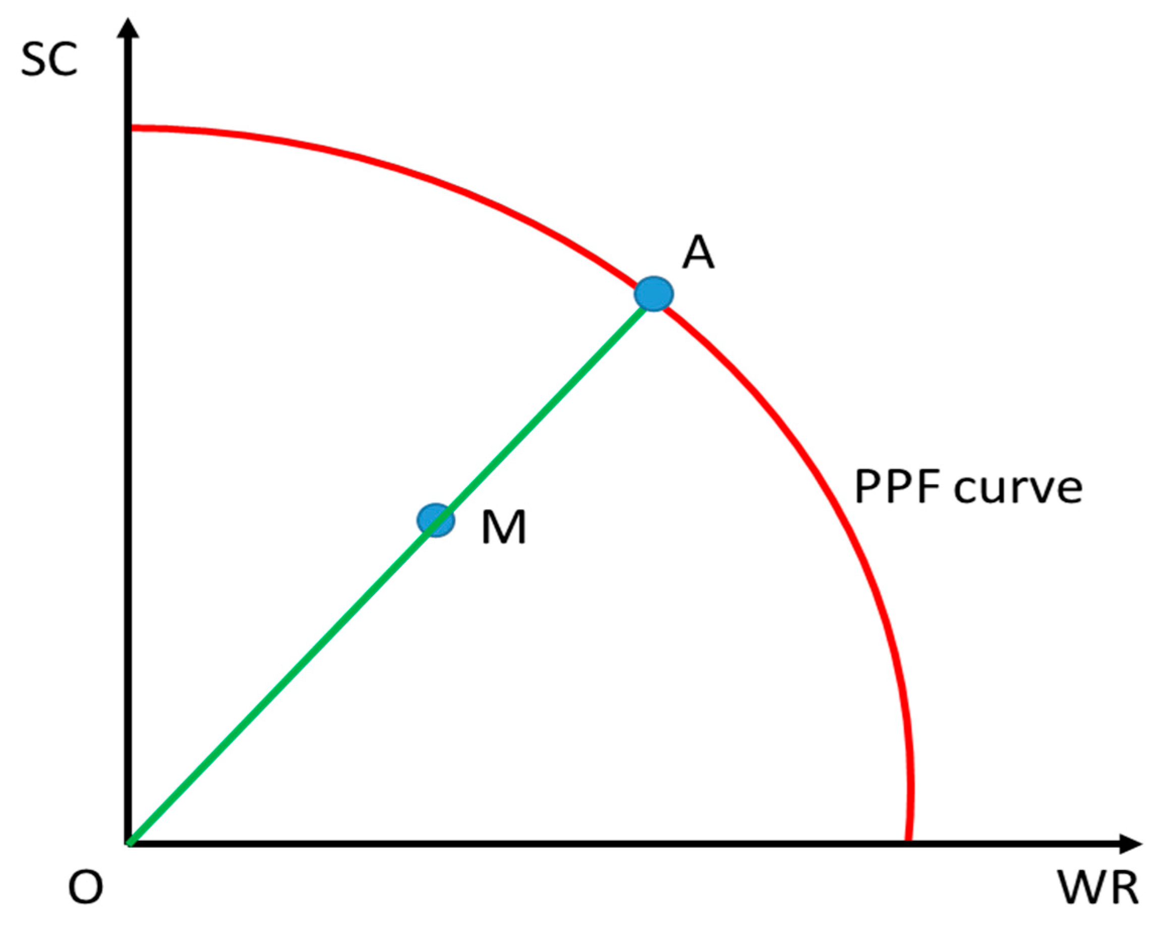
We also took the pair of WR-SC in the period 1990–1995 as an example. After the functional form of the PPF curve was identified, a point with the average value of WR and SC in this period could be found from 50,000 points and was noted as the mean point M. The line that connects the origin O and point M intersects the PPF curve at a point noted as A. The trade-off intensity is defined as the ratio of segment lengths MA and OA (Figure 2). This calculation was performed in GeoGebra Classic [49]. The larger the ratio, the stronger the trade-off relationship between two ES that are compared, implying that the mean point is farther from the PPF curve. The whole approach is illustrated in Figure 3.

3. Results

3.1. Quantity of ES and Temporal Changes

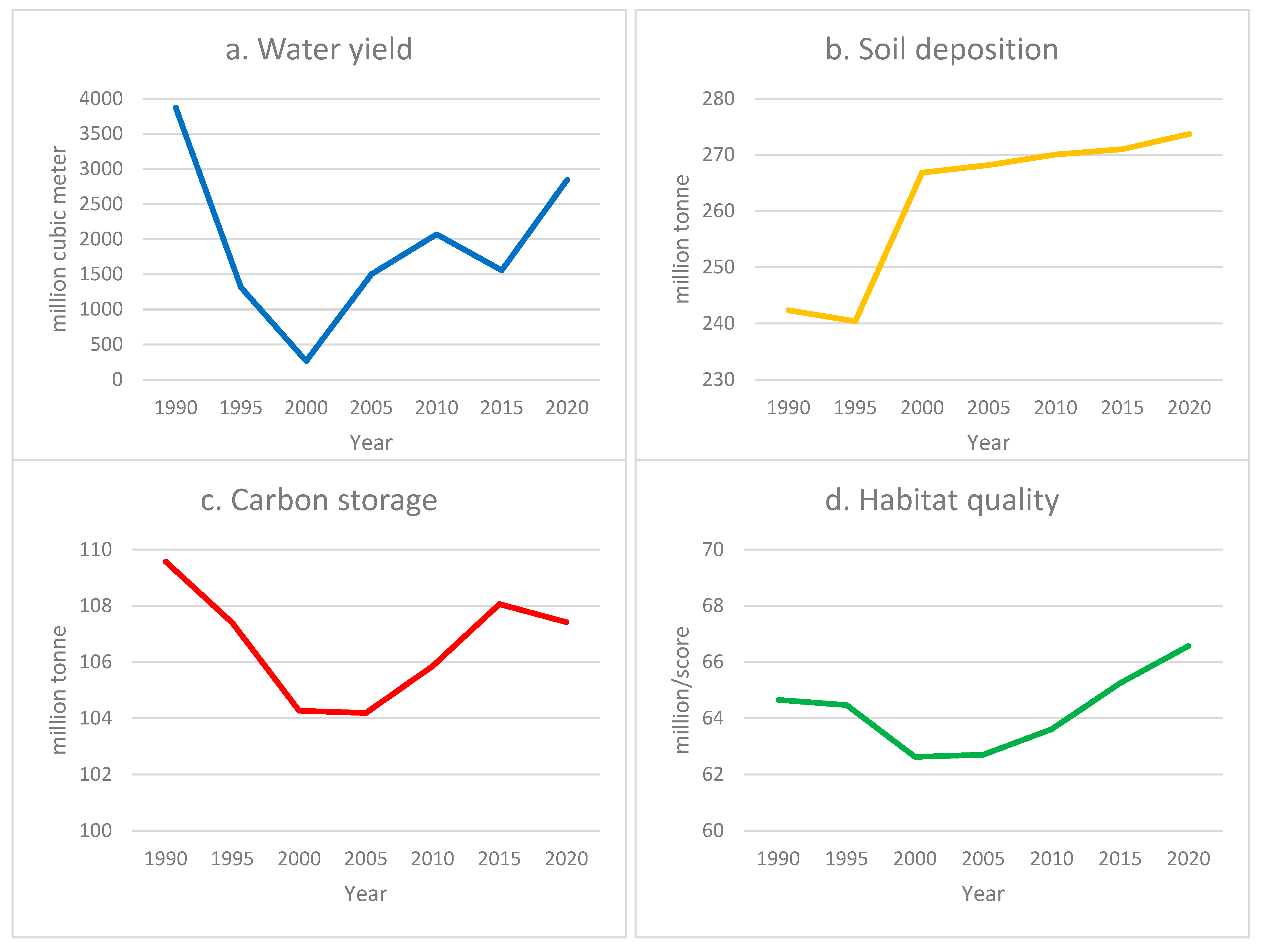
Figure 4 shows the results of InVEST models for four ES over seven years in the WLRB. The water yield service experienced a large fluctuation. There was a sharp decline in 1990–2000, from about 3800 million cubic meters to about 1300 million cubic meters. From 2000 to 2010, it slowly recovered to about 2100 million cubic meters and finally recovered to about 2800 million cubic meters after the turning point in 2015. Overall, the water yield service decreased by about 1000 million cubic meters (Figure 4a). The soil deposition service continually increased year by year after a slight decline in 1995, from about 240 million tons to about 270 million tons, with a total increase of about 30 million tons (Figure 4b). The carbon storage service exhibited a generally stable, slightly fluctuating, and slightly decreasing trend, from about 110 million tons in 1990 to 107 million tons in 2020 (Figure 4c), while the habitat quality service presented an overall stable, slightly fluctuating, and slightly increasing trend, from a score of about 65 million in 1990 to a score of about 67 million in 2020 (Figure 4d). The spatial variations of the four ES at the pixel level can be found in Supplementary Materials Figures S1–S4.
Based on the modeling results, the temporal changes in these four ES are calculated for six periods in the WLRB. The amount of WR varied significantly with periods ranging from −2559 in 1990–1995 to 1287 million m3 in 2015–2020, while the amount of SC, CS, and HI remained relatively stable within the range of ±3 million, except for 26 million tons of SC in 1995–2000 (Table 4). Detailed spatial distributions of the temporal changes at the pixel level can be found in Supplementary Materials Figures S5–S8.

3.2. PPF Curves for Pairwise ES Trade-Offs

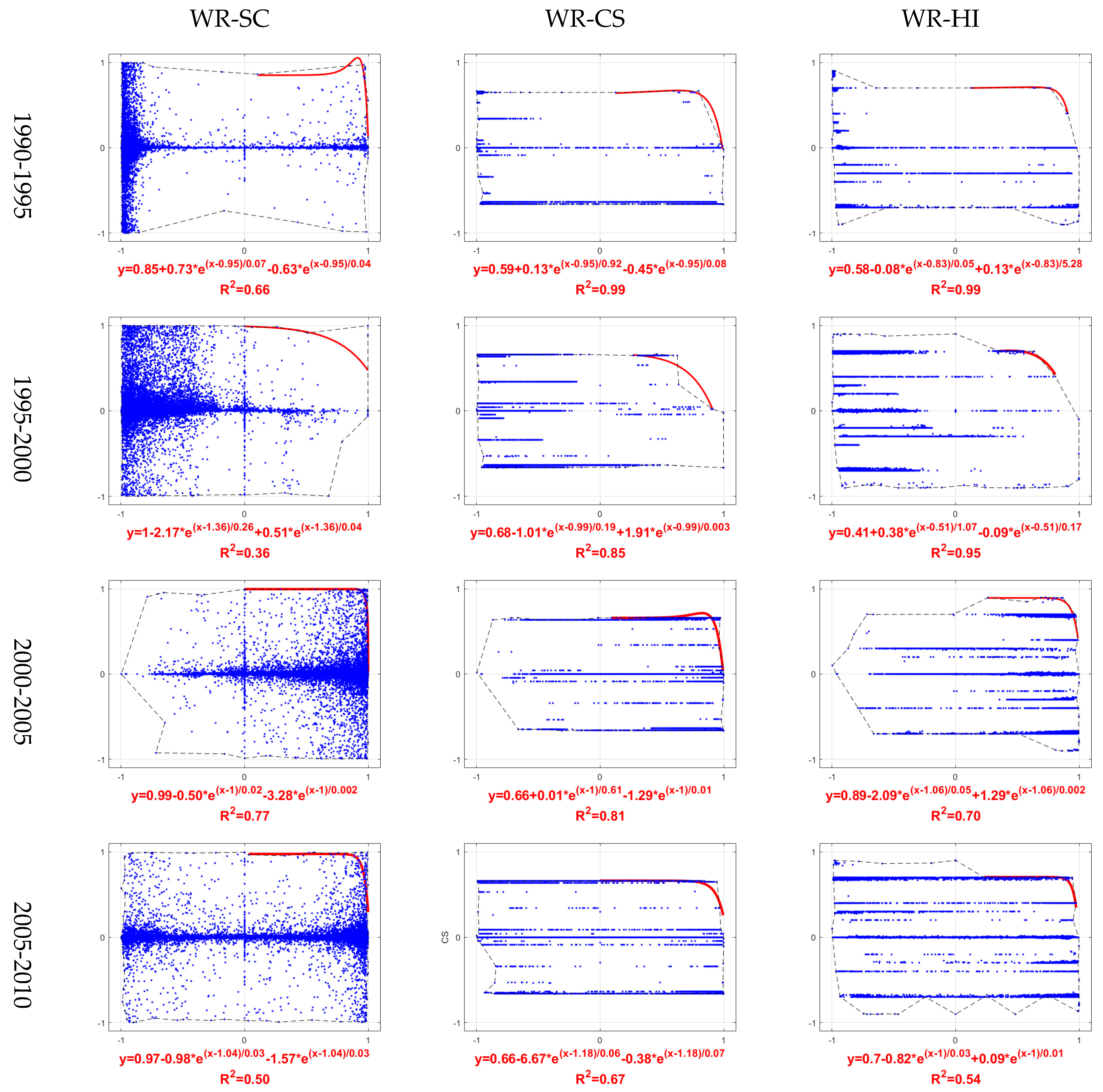
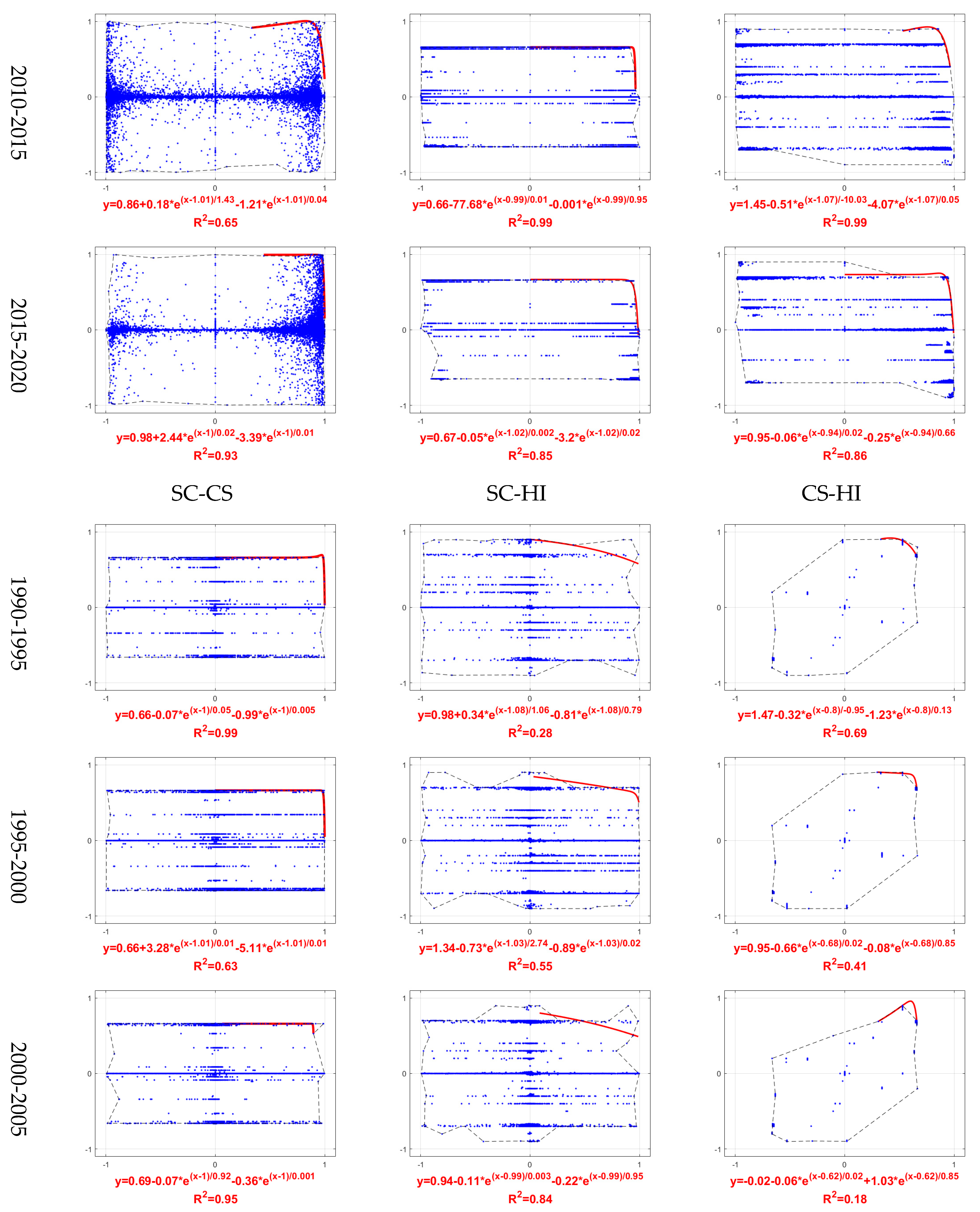
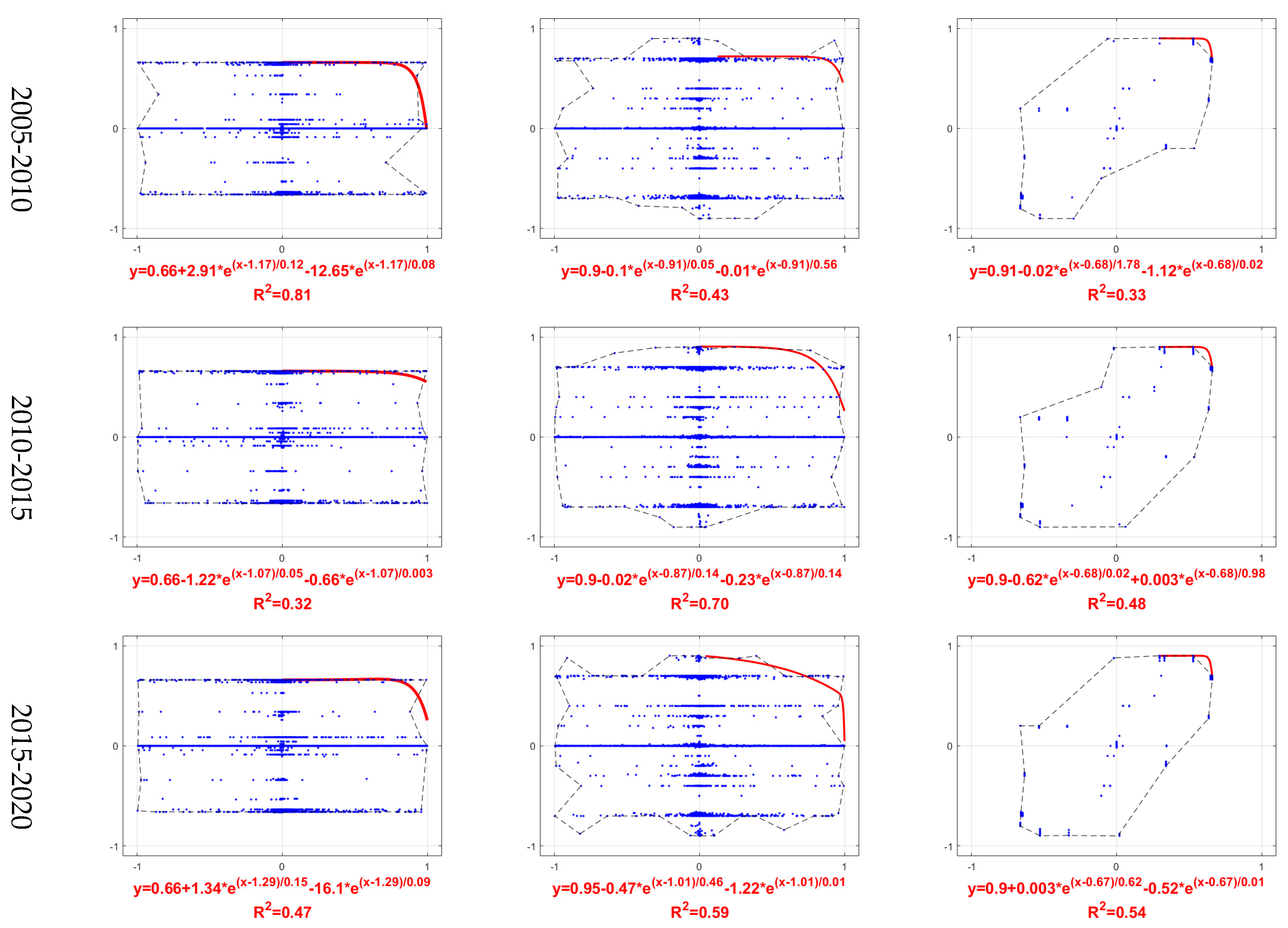
Figure 5 illustrates the PPF curves for six pairs of ES in the WLRB for six periods. The shapes of PPF curves vary with the periods, implying that the biophysical constraints in different years lead to changes in multiple ES, which changes the relationships between ES. In general, a monotonic convex form represents a clear trade-off between two ES, e.g., the relationships between SC and CS in 1990–1995 (column 5 row 1 in Figure 5), meaning that the increase in SC results in a decrease in CS. However, a non-monotonic convex form indicates a more complex relationship between two ES, e.g., the relationship between WR and HI in 2010–2015 (column 3 row 5 in Figure 5), meaning that the synergy and trade-off may simultaneously exist. The increase in WR leads to an increase in HI before a given turning point, and the continuing increase in WR leads to a decrease in HI after that point.

3.3. Changes in Trade-Off Intensity

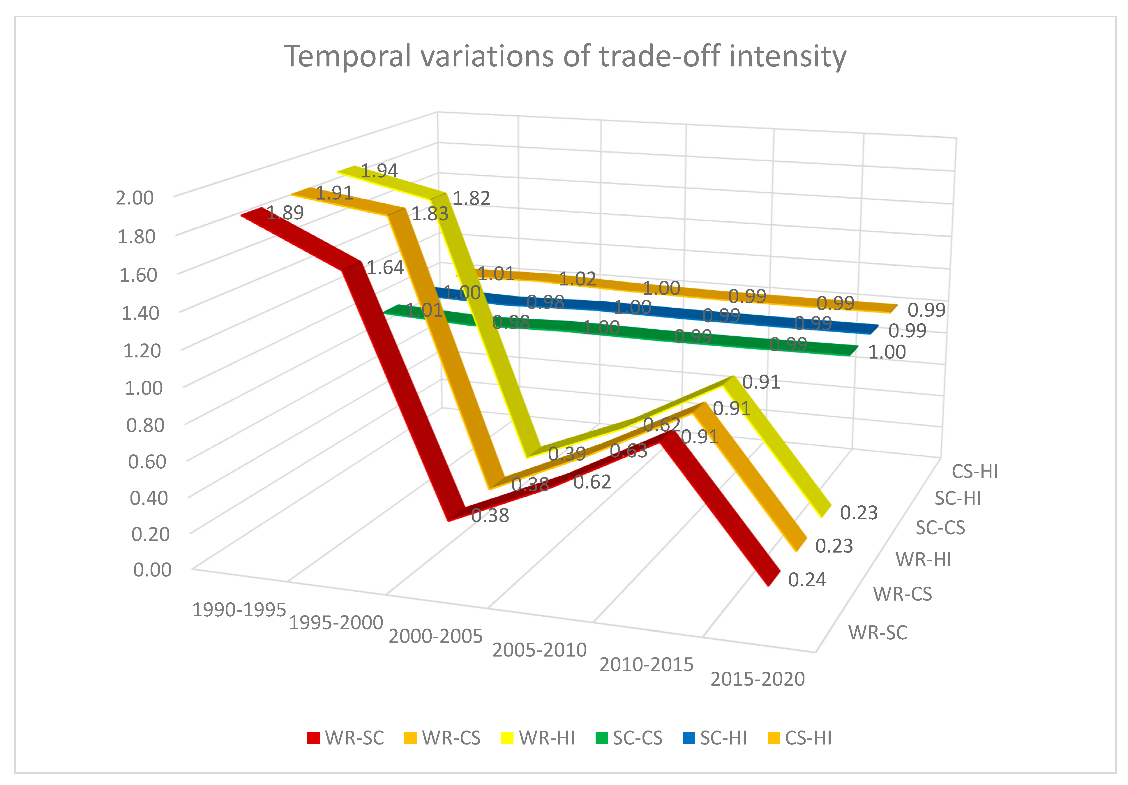
Based on the estimated PPF curves and the mean points of two ES, the trade-off intensity for six pairs of ES during six periods was calculated. Six sequences of trade-off intensity can be grouped into two patterns; the intensities of WR-SC, WR-CS, and WR-HI saw significant fluctuations with an obviously decreasing trend, while the intensities of SC-CS, SC-HI, and CS-HI stabilized at around one (Figure 6). Noticing the quantity of the water yield (Figure 4a) and the temporal changes in water retention (Table 4), this result could possibly be attributed to the drastic changes in WR and the slight fluctuations in SC, CS, and HI. The trade-off intensities related to WR, such as WR-SC, WR-CS, and WR-HI, also exhibit significant variations, while the intensities between SC-CS, SC-HI, and CS-HI remain stable.

4. Discussion

4.1. Approaches for Estimating PPF

The PPF has been increasingly deemed an appropriate tool for representing trade-offs between ES. There mainly exist four approaches for depicting the PPF. Ruijs et al. developed a two-stage semi-parametric estimation approach by non-parametrically estimating the PPF and the distance of each observation to the PPF using the output-oriented robust conditional free disposal hull method in the first stage and parametrically approximating the non-parametric PPF with a flexible translog function in the second stage [24]. This approach was limited to the positive datasets and performance capabilities of soft- and hardware and thus could not deal with negative ES changes with large data amounts. Bryan et al. provided an approach to calculate PPF by the maximizing the land use allocation of the joint production weights of two ES. This approach was dependent on maximum economic potential of land use [27]. Vallet et al. suggested an approach to detect the production possibility set of each pair of ES by plotting ES values against one another where scenario simulations of ES combinations were necessary [8]. Yang et al. adopted an approach to creating PPF by identifying combinations of ES that had the maximum summed total value, thus ignoring a large number of combinations that might have belonged to the production possibility set [29]. Furthermore, the latter two approaches failed to deliver the functional forms of PPF curves.
The approach developed in this paper is easily operational for estimating the PPF curves of ES pairs and calculating the intensities of ES trade-offs, which has the following advantages. First, it is able to derive functional forms of PPF curves, which allow the graphical illustrations of the shape of ES relationships and the quantitative calculations of trade-off intensities. Second, it can deal with the positive or negative values of the ES-derived from modeling results without the need for performing scenario simulations. Third, the calculation of the trade-off intensity is potentially useful for the comparison of ES trade-offs in different time periods or in different geographical regions. The results are mainly limited by the precision of the spatial data adopted and the models for quantifying ES. This approach could further be improved by using more appropriate functional forms for fitting the PPF curves, by developing new methods for calculating the trade-off intensity, or by increasing the number of the sampled value.

4.2. Implications

The approach developed in this paper makes contributions to quantitatively revealing the interactions between ES and to understanding the inherent linkages within ecosystems. Interpreting PPF leads to new insights on ES relationships, but at the price of complexity because much evidences of relationships must be simultaneously considered. For example, some ES pairs show a simple relationship of trade-off (e.g., WR-SC in 1995–2000), but some ES pairs include a turning point where the relationships of synergy and trade-off successively exist (e.g., WR-CS in 2000–2005). Showing the trade-offs between ES by PPF is helpful for providing knowledge on the existence of turning points and complex relationships between certain ES pairs and thus avoiding unintended and large-scale shifts in the provision of ES.
Points inside the PPF in economics represent economically inefficient situations due to the insufficient use of resources or technical constraints etc., while points outside the PPF represent situations that cannot be achieved under current resources or technology [22]. In this study, all of the mean points are inside the PPF curves, suggesting that the current ES combinations are far from efficient and that landscape optimization rarely exists in the river basin. Therefore, the joint improvement of multiple ES can be reached if the targeted ES are corrected and selected. For example, the changes in WR are relevant to the fluctuations of trade-off intensities for ES pairs, including WR, and increasing or stabilizing the provision of WR may lead to the joint improvement of SC, CS, and HI. Combined with simulations of plausible hypothetical scenarios for targeted ES, PPF curves are a useful tool for visualizing the nature of ES relationships and the changes in trade-off intensity, thus supporting decision-makers to identify optimal solutions, which correspond to the shortest path from a point to the PPF curve, and to make land use planning that increase the overall efficiency over multiple ES.
The movement of PPF curves in economics generally results from the increase in resource supply and the progress of production technology etc., in a dynamic economy [22]. Similarly, changing patterns of natural constraints and human activities may move the PPF curves between ES. Therefore, the driving factors that are responsible for the movement of PPF should be identified, involving not only the biophysical drivers of the landscape but, more importantly, the socio-economic drivers in the region [50]. ES relationships provide insightful information about the trade-offs that must be considered when one ES combination is preferred over another, which is supposed to be reflected in societal preferences regarding what is efficient and desirable [51]. Hence, it is needed to integrate socio-economic components into the assessment of ES trade-offs in order to understand the influences of societal choices on and examine stakeholders’ preferences for efficient ES combinations [52].

5. Conclusions

Taking the WLRB in the semi-arid region of China as an example, this study develops an operational approach to estimate the PPF that represents the temporal trade-offs among four key ES, including WR, SC, CS, and HI. Based on the InVEST models, we visualized the spatial patterns of four ES in 1990, 1995, 2000, 2005, 2010, 2015, and 2020, respectively, and calculated their temporal changes over six periods. We then derived the functional forms of PPF curves for six pairs of ES trade-offs and illustrated the temporal variations of the PPF curves in six periods. According to the PPF functions and the mean points of each ES pair in each period, we calculated the trade-off intensities and showed their changing trends over the past 30 years. Compared to the existing approaches for estimating PPF, our approach has the advantages of fitting functional forms of PPF curves, handling both positive and negative values of ES, and calculating trade-off intensities. This study has three implications. First, showing the trade-offs between ES by PPF is helpful for providing knowledge on the existence of turning points and the complex relationships between certain ES pairs, thus avoiding unintended and large-scale shifts in the provision of ES. Second, PPF curves are a useful tool for visualizing the nature of ES relationships and the changes in trade-off intensity, thus supporting decision-makers to identify optimal solutions and make land use planning that can increase the overall efficiency of multiple ES. Third, socioeconomic components should be integrated into the assessment of ES trade-offs in order to understand the influences of societal choices on and examine stakeholders’ preferences for efficient ES combinations.

Supplementary Materials

The following supporting information can be downloaded at: https://www.mdpi.com/article/10.3390/rs15030749/s1, Figure S1: Spatial distributions of water yield from 1990 to 2020, Figure S2: Spatial distributions of soil deposition from 1990 to 2020, Figure S3: Spatial distributions of carbon storage from 1990 to 2020, Figure S4: Spatial distributions of habitat quality from 1990 to 2020, Figure S5: Spatial distributions of WR in six periods, Figure S6: Spatial distributions of SC in six periods, Figure S7: Spatial distributions of CS in six periods, Figure S8: Spatial distributions of HI in six periods.

Author Contributions

Conceptualization, W.J.; methodology, W.J.; software, W.J.; formal analysis, W.J.; data curation, W.J.; writing—original draft preparation, W.J.; writing—review and editing, X.W.; visualization, W.J.; supervision, Y.L.; project administration, G.G.; funding acquisition, G.G. All authors have read and agreed to the published version of the manuscript.

Funding

This research was funded by Inner Mongolia Agricultural University grant number 2021ZD0015 and by National Natural Science Foundation of China grant number 41991233.

Data Availability Statement

Not applicable.

Acknowledgments

This study is supported by the project “Research and technology demonstration on the systematic governance mechanism of mountains, rivers, forests, croplands, lakes, grasslands and sandy lands in the West Liao River Basin” (2021ZD0015) and the project “Interaction mechanism between water cycle process and ecosystem in arid and semi-arid area” (41991233).

Conflicts of Interest

The authors declare no conflict of interest.

References

  1. Millennium Ecosystem Assessment. Ecosystems and Human Well-Being: Synthesis; Island Press: Washington, DC, USA, 2005. [Google Scholar]
  2. Costanza, R.; De Groot, R.; Braat, L.; Kubiszewski, I.; Fioramonti, L.; Sutton, P.; Farber, S.; Grasso, M. Twenty years of ecosystem services: How far have we come and how far do we still need to go? Ecosyst. Serv. 2017, 28, 1–16. [Google Scholar] [CrossRef]
  3. Torres, A.V.; Tiwari, C.; Atkinson, S.F. Progress in ecosystem services research: A guide for scholars and practitioners. Ecosyst. Serv. 2021, 49, 101267. [Google Scholar] [CrossRef]
  4. Aryal, K.; Maraseni, T.; Apan, A. How much do we know about trade-offs in ecosystem services? A systematic review of empirical research observations. Sci. Total. Environ. 2022, 806, 151229. [Google Scholar] [CrossRef]
  5. Cavender-Bares, J.; Polasky, S.; King, E.; Balvanera, P. A sustainability framework for assessing trade-offs in ecosystem services. Ecol. Soc. 2015, 20, 17. [Google Scholar] [CrossRef] [Green Version]
  6. Howe, C.; Suich, H.; Vira, B.; Mace, G.M. Creating win-wins from trade-offs? Ecosystem services for human well-being: A meta-analysis of ecosystem service trade-offs and synergies in the real world. Glob. Environ. Chang. 2014, 28, 263–275. [Google Scholar] [CrossRef] [Green Version]
  7. Cavender-Bares, J.; Balvanera, P.; King, E.; Polasky, S. Ecosystem service trade-offs across global contexts and scales. Ecol. Soc. 2015, 20, 22. [Google Scholar] [CrossRef] [Green Version]
  8. Vallet, A.; Locatelli, B.; Levrel, H.; Wunder, S.; Seppelt, R.; Scholes, R.J.; Oszwald, J. Relationships Between Ecosystem Services: Comparing Methods for Assessing Tradeoffs and Synergies. Ecol. Econ. 2018, 150, 96–106. [Google Scholar] [CrossRef]
  9. Bennett, E.M.; Peterson, G.D.; Gordon, L.J. Understanding relationships among multiple ecosystem services. Ecol. Lett. 2009, 12, 1394–1404. [Google Scholar] [CrossRef]
  10. Birkhofer, K.; Diehl, E.; Andersson, J.; Ekroos, J.; Früh-Müller, A.; Machnikowski, F.; Mader, V.L.; Nilsson, L.; Sasaki, K.; Rundlöf, M.; et al. Ecosystem services—Current challenges and opportunities for ecological research. Front. Ecol. Evol. 2015, 2, 413. [Google Scholar] [CrossRef] [Green Version]
  11. Seppelt, R.; Dormann, C.F.; Eppink, F.V.; Lautenbach, S.; Schmidt, S. A quantitative review of ecosystem service studies: Approaches, shortcomings and the road ahead. J. Appl. Ecol. 2011, 48, 630–636. [Google Scholar] [CrossRef]
  12. Cardinale, B.J.; Duffy, J.E.; Gonzalez, A.; Hooper, D.U.; Perrings, C.; Venail, P.; Narwani, A.; Mace, G.M.; Tilman, D.; Wardle, D.A.; et al. Biodiversity loss and its impact on humanity. Nature 2012, 486, 59–67. [Google Scholar] [CrossRef] [Green Version]
  13. Lu, N.; Liu, L.; Yu, D.; Fu, B. Navigating trade-offs in the social-ecological systems. Curr. Opin. Environ. Sustain. 2021, 48, 77–84. [Google Scholar] [CrossRef]
  14. Koch, E.W.; Barbier, E.B.; Silliman, B.R.; Reed, D.J.; Perillo, G.M.; Hacker, S.D.; Granek, E.F.; Primavera, J.H.; Muthiga, N.; Polasky, S.; et al. Non-linearity in ecosystem services: Temporal and spatial variability in coastal protection. Front. Ecol. Environ. 2009, 7, 29–37. [Google Scholar] [CrossRef]
  15. Liu, L.; Wang, Z.; Wang, Y.; Zhang, Y.; Shen, J.; Qin, D.; Li, S. Trade-off analyses of multiple mountain ecosystem services along elevation, vegetation cover and precipitation gradients: A case study in the Taihang Mountains. Ecol. Indic. 2019, 103, 94–104. [Google Scholar] [CrossRef]
  16. Jaligot, R.; Chenal, J.; Bosch, M. Assessing spatial temporal patterns of ecosystem services in Switzerland. Landsc. Ecol. 2019, 34, 1379–1394. [Google Scholar] [CrossRef]
  17. Zhou, Z.; Robinson, G.M.; Song, B. Experimental research on trade-offs in ecosystem services: The agro-ecosystem functional spectrum. Ecol. Indic. 2019, 106, 105536. [Google Scholar] [CrossRef]
  18. Capriolo, A.; Boschetto, R.; Mascolo, R.; Balbi, S.; Villa, F. Biophysical and economic assessment of four ecosystem services for natural capital accounting in Italy. Ecosyst. Serv. 2020, 46, 101207. [Google Scholar] [CrossRef]
  19. Roy, S.G.; Uchida, E.; de Souza, S.P.; Blachly, B.; Fox, E.; Gardner, K.; Gold, A.J.; Jansujwicz, J.; Klein, S.; McGreavy, B.; et al. A multiscale approach to balance trade-offs among dam infrastructure, river restoration, and cost. Proc. Natl. Acad. Sci. USA 2018, 115, 12069–12074. [Google Scholar] [CrossRef] [PubMed] [Green Version]
  20. O’Connell, C.S.; Carlson, K.M.; Cuadra, S.; Feeley, K.J.; Gerber, J.S.; West, P.C.; Polasky, S. Balancing tradeoffs: Reconciling multiple environmental goals when ecosystem services vary regionally. Environ. Res. Lett. 2018, 13, 064008. [Google Scholar] [CrossRef]
  21. Ager, A.A.; Houtman, R.M.; Day, M.A.; Ringo, C.; Palaiologou, P. Tradeoffs between US national forest harvest targets and fuel management to reduce wildfire transmission to the wildland urban interface. For. Ecol. Manag. 2019, 434, 99–109. [Google Scholar] [CrossRef]
  22. Varian, H.R. Intermediate Microeconomics: A Modern Approach, 8th ed.; W.W. Norton & Co: New York, NY, USA, 2010. [Google Scholar]
  23. Bekele, E.G.; Lant, C.L.; Soman, S.; Misgna, G. The evolution and empirical estimation of ecological-economic production possibilities frontiers. Ecol. Econ. 2013, 90, 1–9. [Google Scholar] [CrossRef]
  24. Ruijs, A.; Wossink, A.; Kortelainen, M.; Alkemade, R.; Schulp, C. Trade-off analysis of ecosystem services in Eastern Europe. Ecosyst. Serv. 2013, 4, 82–94. [Google Scholar] [CrossRef]
  25. Bagdon, B.A.; Huang, C.-H.; Dewhurst, S.; Meador, A.S. Climate Change Constrains the Efficiency Frontier When Managing Forests to Reduce Fire Severity and Maximize Carbon Storage. Ecol. Econ. 2017, 140, 201–214. [Google Scholar] [CrossRef]
  26. Pohjanmies, T.; Eyvindson, K.; Triviño, M.; Mönkkönen, M. More is more? Forest management allocation at different spatial scales to mitigate conflicts between ecosystem services. Landsc. Ecol. 2017, 32, 2337–2349. [Google Scholar] [CrossRef]
  27. Bryan, B.A.; Crossman, N.D.; Nolan, M.; Li, J.; Navarro, J.; Connor, J.D. Land use efficiency: Anticipating future demand for land-sector greenhouse gas emissions abatement and managing trade-offs with agriculture, water, and biodiversity. Glob. Chang. Biol. 2015, 21, 4098–4114. [Google Scholar] [CrossRef]
  28. Li, R.; Li, R.; Zheng, H.; Yang, Y.; Ouyang, Z. Quantifying Ecosystem Service Trade-Offs to Inform Spatial Identification of Forest Restoration. Forests 2020, 11, 563. [Google Scholar] [CrossRef]
  29. Yang, W.; Jin, Y.; Sun, T.; Yang, Z.; Cai, Y.; Yi, Y. Trade-offs among ecosystem services in coastal wetlands under the effects of reclamation activities. Ecol. Indic. 2018, 92, 354–366. [Google Scholar] [CrossRef]
  30. Liu, X.; Xu, Z.; Yu, R. Spatiotemporal variability of drought and the potential climatological driving factors in the Liao River basin. Hydrol. Process. 2012, 26, 1–14. [Google Scholar] [CrossRef]
  31. Zhong, Y.; Zhong, M.; Feng, W.; Zhang, Z.; Shen, Y.; Wu, D. Groundwater Depletion in the West Liaohe River Basin, China and Its Implications Revealed by GRACE and In Situ Measurements. Remote Sens. 2018, 10, 493. [Google Scholar] [CrossRef] [Green Version]
  32. Zhu, Y.-H.; Zhang, S.; Sun, B.; Xi, X.-K.; Liu, Y.; Shi, X.-H. Spatial variability of soil organic carbon in the West Liao River Basin. Isr. J. Ecol. Evol. 2018, 64, 25–34. [Google Scholar] [CrossRef]
  33. Zhao, H.; Wang, Z.; Li, X.; Chu, Z.; Zhao, C.; Zhao, F. Research on the evolution characteristics of future climate change in West Liao River Basin. Environ. Sci. Pollut. Res. 2022, 29, 509–517. [Google Scholar] [CrossRef] [PubMed]
  34. Gao, Z.; He, J.; Dong, K.; Li, X. Trends in reference evapotranspiration and their causative factors in the West Liao River basin, China. Agric. For. Meteorol. 2017, 232, 106–117. [Google Scholar] [CrossRef]
  35. ArcGIS Desktop, version 10.6; ESRI: Redlands, CA, USA, 2018.
  36. NASA: Digital Elevation Model. Available online: https://asterweb.jpl.nasa.gov/GDEM.asp (accessed on 27 January 2023).
  37. Zhang, X.; Liu, L.; Chen, X.; Gao, Y.; Xie, S.; Mi, J. GLC_FCS30: Global land-cover product with fine classification system at 30 m using time-series Landsat imagery. Earth Syst. Sci. Data 2021, 13, 2753–2776. [Google Scholar] [CrossRef]
  38. Yue, T.; Yin, S.; Xie, Y.; Yu, B.; Liu, B. Rainfall erosivity mapping over mainland China based on high density hourly rainfall records. Earth Syst. Sci. Data 2022, 14, 665–682. [Google Scholar] [CrossRef]
  39. Yang, Q. Soil Erodibility Dataset of Pan-Third Pole 20 Countries; National Tibetan Plateau Data Center: Beijing, China, 2021. [Google Scholar]
  40. Peng, S. 1-km Monthly Precipitation Dataset for China (1901–2020); National Tibetan Plateau Data Center: Beijing, China, 2020. [Google Scholar]
  41. Peng, S. (1 km Monthly Potential Evapotranspiration Dataset in China (1990–2020); National Tibetan Plateau Data Center: Beijing, China, 2022. [Google Scholar]
  42. Hengl, T.; De Jesus, J.M.; Heuvelink, G.B.M.; Gonzalez, M.R.; Kilibarda, M.; Blagotić, A.; Shangguan, W.; Wright, M.N.; Geng, X.; Bauer-Marschallinger, B.; et al. SoilGrids250m: Global gridded soil information based on machine learning. PLoS ONE 2017, 12, e0169748. [Google Scholar] [CrossRef] [PubMed] [Green Version]
  43. Poggio, L.; de Sousa, L.M.; Batjes, N.H.; Heuvelink, G.B.M.; Kempen, B.; Ribeiro, E.; Rossiter, D. SoilGrids 2.0: Producing soil information for the globe with quantified spatial uncertainty. Soil 2021, 7, 217–240. [Google Scholar] [CrossRef]
  44. National Catalogue Service for Geographic Information: Railroad. Available online: https://www.webmap.cn (accessed on 27 January 2023).
  45. National Catalogue Service For Geographic Information: Road. Available online: https://www.webmap.cn, (accessed on 27 January 2023).
  46. InVEST, version 3.12; Natural Capital Project: Stanford, CA, USA, 2022.
  47. Stanford University; University of Minnesota; Chinese Academy of Sciences; The Nature Conservancy; World Wildlife Fund; Stockholm Resilience Centre. User’s Guide; 2022. Available online: https://storage.googleapis.com/releases.naturalcapitalproject.org/invest-userguide/latest/index.html, (accessed on 12 May 2022).
  48. Matlab, version R2021b; MathWorks: Galway, Ireland, 2021.
  49. GeoGebra Classic; GeoGebra: Linz, Austria, 2022.
  50. Turkelboom, F.; Leone, M.; Jacobs, S.; Kelemen, E.; García-Llorente, M.; Baró, F.; Termansen, M.; Barton, D.N.; Berry, P.; Stange, E.; et al. When we cannot have it all: Ecosystem services trade-offs in the context of spatial planning. Ecosyst. Serv. 2018, 29, 566–578. [Google Scholar] [CrossRef]
  51. Goldstein, J.H.; Caldarone, G.; Duarte, T.K.; Ennaanay, D.; Hannahs, N.; Mendoza, G.; Polasky, S.; Wolny, S.; Daily, G.C. Integrating ecosystem-service tradeoffs into land-use decisions. Proc. Natl. Acad. Sci. USA 2012, 109, 7565–7570. [Google Scholar] [CrossRef] [Green Version]
  52. King, E.; Cavender-Bares, J.; Balvanera, P.; Mwampamba, T.H.; Polasky, S. Trade-offs in ecosystem services and varying stakeholder preferences: Evaluating conflicts, obstacles, and opportunities. Ecol. Soc. 2015, 20, 25. [Google Scholar] [CrossRef]
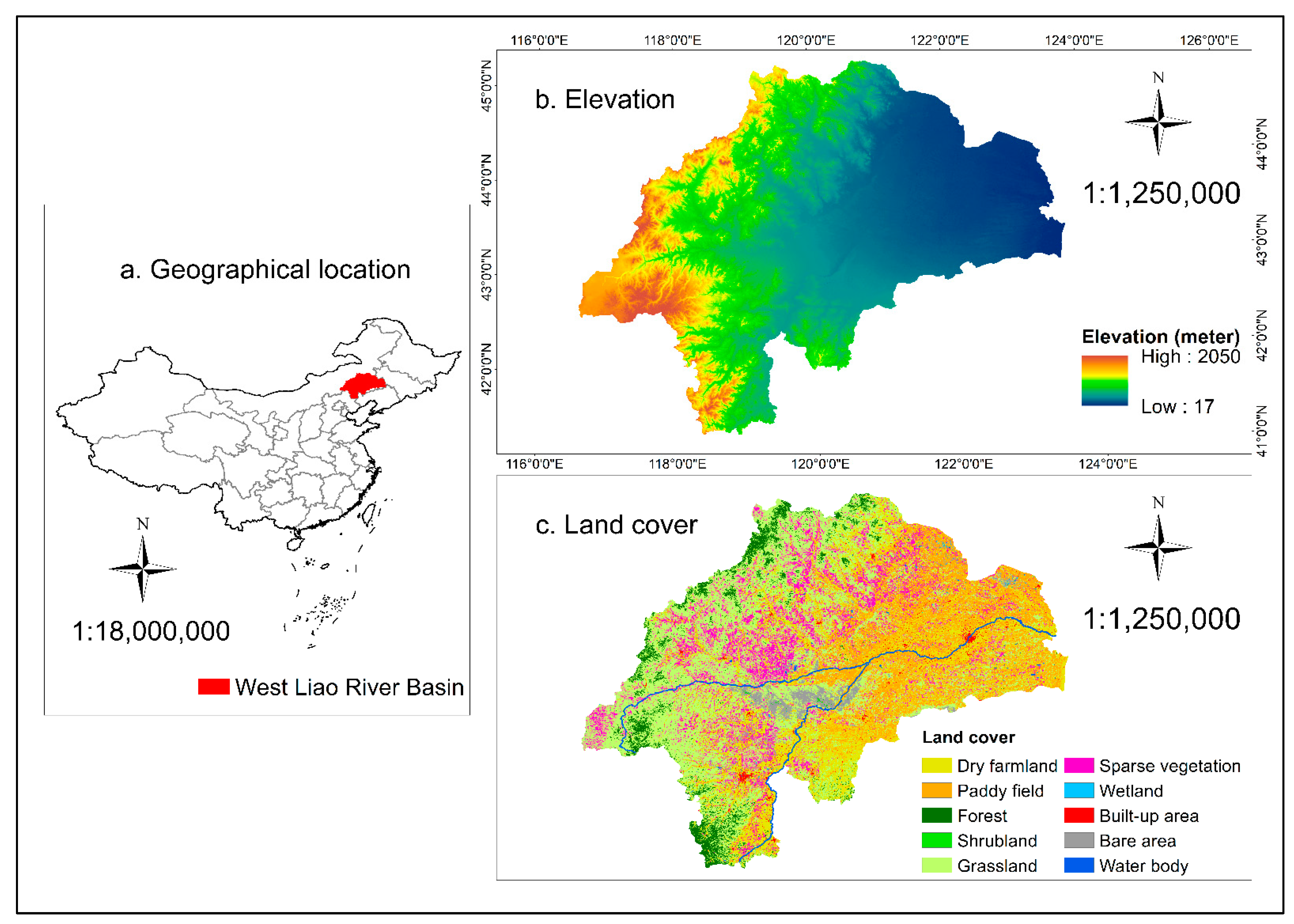
Figure 1. (a) Geographical location, (b) Elevation, and (c) Land cover of the West Liao River Basin.
Remotesensing 15 00749 g001
Figure 2. The schematic diagram for the calculation of trade-off intensity.
Remotesensing 15 00749 g002
Figure 3. The approach for fitting PPF curves and calculating trade-off intensity.
Remotesensing 15 00749 g003
Figure 4. Temporal changes in (a) Water yield, (b) Soil deposition, (c) Carbon storage, and (d) Habitat quality from 1990 to 2020.
Remotesensing 15 00749 g004
Figure 5. Production possibility frontier curves for six pairs of ecosystem services in six periods.
Remotesensing 15 00749 g005aRemotesensing 15 00749 g005bRemotesensing 15 00749 g005c
Figure 6. Trade-off intensity for six pairs of ecosystem services in six periods.
Remotesensing 15 00749 g006
Table 1. Multi-source spatial data.
DataTypeResolutionSourceReference
Digital Elevation ModelRaster30 m × 30 mhttps://asterweb.jpl.nasa.gov/GDEM.asp
(accessed on 27 January 2023)
[36]
Land Use/Land CoverRaster30 m × 30 mhttps://data.casearth.cn
(accessed on 27 January 2023)
[37]
Rainfall ErosivityRaster1 km × 1 kmhttp://clicia.bnu.edu.cn/data
(accessed on 27 January 2023)
[38]
Soil ErodibilityRaster250 m × 250 mhttp://data.tpdc.ac.cn
(accessed on 27 January 2023)
[39]
PrecipitationRaster1 km × 1 kmhttp://data.tpdc.ac.cn
(accessed on 27 January 2023)
[40]
EvapotranspirationRaster1 km × 1 kmhttp://data.tpdc.ac.cn
(accessed on 27 January 2023)
[41]
Soil DepthRaster250 m × 250 mhttps://data.isric.org
(accessed on 27 January 2023)
[42]
Volumetric Water ContentRaster250 m × 250 mhttps://data.isric.org
(accessed on 27 January 2023)
[43]
RailroadVector1:250000https://www.webmap.cn
(accessed on 27 January 2023)
[44]
RoadVector1:250000https://www.webmap.cn
(accessed on 27 January 2023)
[45]
Table 2. Quantifying methods of InVEST models.
ESModelAlgorithmDescription
Water yieldAnnual Water Yield W i = ( 1 A E T i P i ) × P i Pi refers to the annual precipitation (mm/yr) on pixel i, AETi refers to the annual actual evapotranspiration (mm/yr) on pixel i, and AETi/Pi refers to the approximation of the Budyko curve.
Soil depositionSediment Delivery Ratio S i = A i × ( 1 S D R i )   A i = R i × K i × L S i × C i × S P i   S D R i = S D R m a x 1 + e ( I C 0 I C i / k ) Ai refers to the amount of annual soil loss (ton/ha/yr) on pixel i, given by the revised universal soil loss equation, where Ri is the rainfall erosivity factor (MJ•mm/ha/hr/yr), Ki is the soil erodibility factor (ton•ha•hr/MJ/ha/mm), LSi (unitless) is the slope length-gradient factor, Ci (unitless) is the cover management factor; and SPi (unitless) is the support practice factor.
SDRi refers to the sediment deliver ratio for pixel i derived from the conductivity index, where SDRmax is the maximum theoretical SDR; IC0 and k define the shape of the SDR-IC relationship.
Carbon storageCarbon Storage and Sequestration C i = C a + C b + C s + C d Ca is aboveground biomass (ton/ha), Cb is belowground biomass (ton/ha), Cs is soil carbon storage (ton/ha), Cd is dead organic matter (ton/ha).
Habitat qualityHabitat Quality Q i j = H j × ( 1 D i j z D i j z + m z ) Hj refers to the habitat suitability of land use type j, Dij is the total threat level for land use type j on pixel i, and m is half of the maximum value of Dij.
Table 3. The interpretation of temporal ES changes.
ChangePositiveNegative
Water yield (m3)Water retentionWater loss
Soil deposition (tons)Soil conservationSoil loss
Carbon storage (tons)Carbon sequestrationCarbon emission
Habitat quality (score)Habitat improvementHabitat degradation
Table 4. Temporal changes of water retention, soil conservation, carbon sequestration, and habitat improvement in six periods.
ES change1990–19951995–20002000–20052005–20102010–20152015–2020
WR (million m3)−2559.42−1049.111234.51568.58−512.021287.38
SC (million tons)−1.9426.421.371.860.972.70
CS (million tons)−2.18−3.12−0.081.662.21−0.64
HI (million/score)−0.18−1.840.070.911.641.33
Disclaimer/Publisher’s Note: The statements, opinions and data contained in all publications are solely those of the individual author(s) and contributor(s) and not of MDPI and/or the editor(s). MDPI and/or the editor(s) disclaim responsibility for any injury to people or property resulting from any ideas, methods, instructions or products referred to in the content.