Abstract
Soil moisture is a key parameter in hydrological research and drought management. The inversion of soil moisture based on land surface temperature (LST) and NDVI triangular feature spaces has been widely used in various studies. Remote sensing provides regional LST data with coarse spatial resolutions which are insufficient for field scale (tens of meters). In this study, we bridged the data gap by adopting a Data Mining Sharpener algorithm to downscale MODIS thermal data with Vis-NIR imagery from Sentinel-2. To evaluate the downscaling algorithm, an unmanned aerial system (UAS) equipped with a thermal sensor was used to capture the ultra-fine resolution LST at three sites in the Tang River Basin in China. The obtained fine-resolution LST data were then used to calculate the Temperature Vegetation Dryness Index (TVDI) for soil moisture monitoring. Results indicated that downscaled LST data from satellites showed spatial patterns similar to UAS-measured LST, although discrepancies still existed. Based on the fine-resolution LST data, a 10-m resolution TVDI map was generated. Significant negative correlations were observed between the TVDI and in-situ soil moisture measurements (Pearson’s r of and ). Overall, the fine-resolution TVDI derived from the downscaled LST has a high potential for capturing spatial soil moisture variation.
1. Introduction
As a key variable of the climate system, soil moisture (SM) affects the water, energy, and biogeochemical cycles [1]. Mapping large-scale soil moisture with a fine temporal and spatial resolution is, therefore, critical to many scientific studies and applications, such as climate prediction, crop growth modeling, and droughts forecasting [2,3,4]. Particularly in the agricultural field, soil moisture is considered one potential resource for agricultural drought monitoring, which is vital for food security [5].
In general, SM can be estimated in two ways: through in-situ measurements or via remote sensing data [6,7]. The conventional in-situ measurement is the most accurate; however, this is laborious, time-consuming, and lacks representativeness, making it unsuitable at the regional scale [8,9]. On the other hand, remote sensing methods are promising since they can provide an effective way to monitor large-scale SM at a low cost. Nevertheless, the estimation of SM by remote sensing involves a number of parameters (e.g., land cover and surface roughness), whose uncertainty reduces retrieval accuracy. Thus, it is crucial to calibrate and validate SM remote sensing products using in-situ measurements. The emergence of new remote sensing methods, such as the GNSS—reflectometry in field scale [10], as well as radiometry [11] show high potential to improve the accuracy.
Remote sensing techniques enable monitoring SM through microwave methods or optical (visible and infrared)/TIR methods [12]. Microwave-based remote sensing is recognized as one of the best ways for global monitoring of SM because it is sensitive to SM and unaffected by atmospheric conditions [13]. The existing products derived from active and passive microwave satellites can provide large-scale SM estimates, e.g., Advanced Scatterometer (ASCAT) [14], the Soil Moisture Active and Passive (SMAP) [15], and the European Space Agency’s Climate Change Initiative (ESA CCI) [16]. It should be noted, however, that these microwave products are limited by vegetation and surface roughness [17], as well as their coarse resolution, which limits their applicability in many studies.
Optical-based remote sensing uses the spectral reflectance properties of soil and vegetation [18], which has great potential to indirectly estimate soil moisture with finer spatial resolutions. A number of studies have been conducted to establish the empirical relationships between SM and the soil reflectivity/vegetation indexes extracted from the optical bands [19,20,21,22]. Most of these studies have failed to address the apparent time lag between vegetation indexes and the actual moisture state, and other factors like temperature and soil properties are not taken into account. TIR-based remote sensing, on the other hand, can effectively generate land surface temperature (LST) to monitor changes in soil thermal properties under bare soil and sparsely vegetated surfaces, which can be used to derive SM [23,24]. However, in dense vegetation area, the LST is more representative of vegetation temperature and it is difficult to obtain soil temperature to invert SM. Synergistic use of optical and TIR bands is an important direction, which could provide vegetation water stress conditions and SM information. One of the most well-known approaches is the “trapezoid” or “triangle” method [25,26]. The temperature vegetation dryness index (TVDI), proposed by Sandholt et al. [27], is based on a triangle feature space established using a scatterplot of LST and a normalized difference vegetation index (NDVI). TVDI can represent the relative soil moisture [28] and is widely used as a soil moisture indicator [2,29,30].
So far, the optical and TIR data have been available from multiple sources. For instance, the Moderate Resolution Imaging Spectroradiometer (MODIS) provides the NDVI at a 250-m resolution and LST at a 1-km resolution, and Landsat 8 satellite provides NDVI at a 30-m resolution and LST at a 100-m resolution. Due to the resolution trade-off and the lower number of thermal sensors, current satellite missions cannot provide as detailed TIR images as visible and NIR images do [31,32]. The most commonly used method to enhance the spatial resolution of the satellite LST is statistical downscaling (also called thermal sharpening), which enhances the resolution of the LST by using spatially distributed auxiliary data that are statistically correlated to the LST [32]. A number of sharpening methods have been applied for sharpening coarse spatial resolution TIR data with higher spatial resolution Vis-NIR observations, such as DisTrad [33], STARFM [34], TsHARP [35], Artificial Neural Networks [36], the Data Mining Sharpener (DMS) [37], and NL-DisTrad [38]. The sharpening method can also take advantage of multiple satellite data. For example, MODIS/COPERNICUS Sentinel-3 TIR images with Sentinel-2 Vis-NIR images together could provide LST at fine spatial and temporal resolutions [39,40].
Despite the growth in studies of downscaling methods, the evaluation of thermal sharpening techniques has traditionally been performed with cross-validation on the original Landsat or ASTER TIR-derived LST products, which have spatial resolutions of 60–100 m and 90 m, respectively [39], making it difficult to meet the needs of evaluating sharpening to 30 m or even 10 m. To verify the effect of downscaling methods, the finer resolution thermal image is required as a reference. Unmanned aerial systems (UAS) equipped with compact sensors can potentially bridge the scale gap between satellite and ground-based observations. The unique advantages, such as economy, flexibility, high accessibility, and high spatial resolution, make UAS remote sensing an increasingly popular technique [41].
Relying on fine-resolution LST data based on downscaling algorithms, soil moisture products with a finer spatial resolution (e.g., 10–30 m) can be obtained. Bai et al. [39] acquired the 30-m resolution LST product by blending Landsat and MODIS data and then used a downscaled LST successfully to estimate the SM of two fields in north China based on the temperature vegetation index method. Ahmed et al. [35] introduced both data fusion and random forest models by integrating multi-source data (including the fused data with MODIS LST and the Landsat LST) to generate daily SM at 30 m × 30 m in the Haihe basin in north China. In order to capture detailed (extremely fine resolution) SM spatial variability within two pro-glacial valleys in the Cordillera Blanca, Peru, Oliver et al. [42] used a UAS with sub-meter resolution multi-spectral sensors to measure the SM based on the TVDI method. The principal limitation of the experimental approach is that the TVDI method requires a study region with large variations in the NDVI and SM [12], a requisite not always met by UAS images. On the other hand, satellite data, with its large-scale and long-term measurements, will become an ideal source for TVDI-based SM monitoring. Taken together, detailed large-scale soil moisture monitoring could be performed by using finer-resolution TVDI data derived from downscaled LST.
In this context, the objectives of this study were to (1) produce a fine-resolution LST by downscaling MODIS TIR data using the DMS algorithm; (2) compare the downscaled result with UAS TIR imagery; (3) estimate TVDI values based on the NDVI and downscaled LST; (4) evaluate the performance of the downscaled TVDI to monitor SM using in-situ measurements.
2. Study Area and Data Preparation
2.1. Study Area
The Tang River Basin in China is a 4200 square kilometers watershed, which is located in the mid-temperate zone and features a continental monsoon climate. Annual precipitation is about 530–660 mm, with the majority of precipitation falling as rain during the summer. The main cropping pattern in the basin comprises winter wheat and summer maize. The proposed LST downscaling method was applied over an experimental area in the middle of the Tang River basin (between longitudes 11440E and 11510E and latitudes 3850N and 3910N, covering 780 km). Figure 1a,b show the location of the study area within the Tang River basin in Hebei Province in north China. From the digital elevation model (DEM) map and geomorphological map [43] in Figure 1c,d, the study area is characterized by mountains, hills, and plains, with elevations ranging from 85 to 1100 m. According to the China Meteorological Data Service Centre, the temperature of August 2021 for the whole region varied between 17 °C and 32 °C. In addition, the mean precipitation was 133 mm in August.
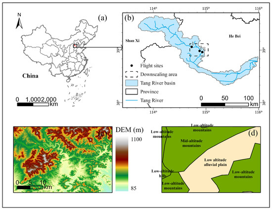
Figure 1.
(a) Location map of Tang River basin in China; (b) Location map of the downscaling area in the Tang river basin; (c) The elevation map of the downscaling area; (d) Geomorphological map of the downscaling area.
In the downscaling area, three flight sites with cropland and grassland land cover were selected for thermal validation. The flight sites used for validation lie along the Tang River (dark blue line). The first site (3859N, 11452E) is a relatively dense corn farmland close to the Gu Daokou village. The second site (393N, 11443E) is a mixed farmland with variable vegetation covers, including bare land, corn, and grass, close to the Xi Shenggou village. The third site (3857N, 11455E) belongs to a hillside covered with uniform grass, and it is located near the Xi Dabei village.
2.2. Satellite Data
In this study, both fine-resolution optical data and coarse-resolution thermal data were used. The fine-resolution optical data were obtained from the COPERNICUS/Sentinel-2 mission. This Sentinel-2 product provides 14 spectral bands with multiple spatial resolutions of 10 m, 20 m, and 60 m. In the downscaling workflow, only the 10-m resolution bands 2, 3, 4 (490–665 nm), and 8 (842 nm) were adopted. Additionally, Bands 4 and 8 were used to calculate the NDVI. To carry on the analysis, the Level-2A atmospherically-corrected image taken on 5 August 2021 was used. Cloud masking was performed to exclude bad-quality data in the image using the s2cloudless dataset, which provides the cloud probability for each pixel based on a machine learning algorithm. The coarse-resolution thermal data were taken from the MODIS MOD11A1 product (Collection 6) on 7 August 2021, near the Sentinel-2 overpassing date. The SRTM 30-m DEM products were adopted for the LST correction. All these satellite data were preprocessed and downloaded using the Google Earth Engine platform (https://developers.google.com/earth-engine, accessed on 25 November 2022).
2.3. UAS Data
We used a DJI Phantom 4 Pro UAS to collect RGB optical data and a DJI Matrice 600 Pro UAS equipped with a thermal camera to collect TIR imagery. DJI Matrice 600 Pro is a six-rotor UAS equipped with a FLIR Tau 2 640 thermal camera from FLIR Systems, USA (focal length 13 mm; F/1.25; Thermal Sensitivity: 50 mK) characterized by an image dimension of 640 × 512 pixels and an FOV of 45× 37. With a 50-m height above ground level, the TIR flights provided approximately a 10-cm resolution. Visible and thermal ground control points (GCPs) were established prior to UAS flights at the two study sites. In the later orthomosaic generation process, GCPs were used to improve image alignment. Following Oliver et al. [42], thermal GCPs were 30-cm foam boards with white squares on a black background and insulating coats on the downward sides. The UAS survey campaigns were performed on 5 August 2021, 6 August 2021, and 7 August 2021 in three flight sites, respectively. In clear sky conditions, the duration of the DJI Matrice 600 Pro campaign was approximately 1 h. The total flight lasted approximately 2–3 h for each site, between 10:00 and 15:00. The overlap between the RGB and TIR images was 85% when flying at 3 m/s. Before constructing the orthomosaic TIR imagery, we conducted a non-uniformity drift compensation caused by an uncooled thermal camera. The processing was completed using the general workflow implemented in Agisoft PhotoScan software.
2.4. In-Situ SM Measurements
During flights, in-situ soil moisture was measured at two sites (34 points at Site 2, and 29 points at Site 3) within the survey area. The position of each sampling point was recorded with a GPS. Each soil moisture measurement is an average of three SM samples taken within a 10 cm radius of each survey point location at a depth of 0–10 cm with an MP406 Moisture Probe. Using the standing wave principle, the MP406 sensor (ICT International Pty Ltd., Armidale, Australia) can measure moisture content by detecting changes in the soil’s dielectric constant as water content changes. The MP406 sensor measurements were positively tested in comparison with gravimetric measurements and calibrated to the volumetric soil moisture using soil samples under different moisture conditions at the sites. As the ground measurement points were shadowed by cornfields and there were many irrigated areas with saturated SM, Site 1 was not suitable for SM sampling. Therefore, in-situ SM measurements were only conducted at the mixed farmland of Site 2 and the uniform grassland of Site 3.
3. Methods
3.1. Experimental Procedure
The flowchart in Figure 2 illustrates the process of evaluating the downscaled TVDI to monitor SM with in-situ data in detail. The following steps were carried out to achieve the main objectives of this study.
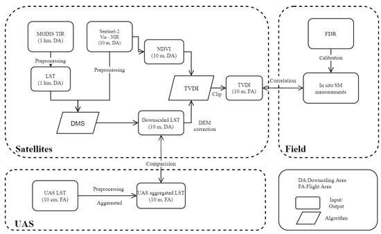
Figure 2.
Flowchart of this study.
Step 1: First, the 1-km resolution TIR data from MODIS and the 10-m resolution Vis-NIR data from Sentinel-2 after preprocessing were input into the DMS model to obtain downscaled 10-m LST (Section 3.2). The preprocessing included cloud masking, band calculation, and re-projection.
Step 2: The UAS TIR images were obtained to construct the orthomosaic UAS LST images at three flight sites. For comparison, 10-cm orthomosaic LST images of UAS were aggregated to the 10-m resolution as downscaled LST data based on the Stefan-Boltzmann law, following Gao et al. [37].
Step 3: The NDVI was calculated using the NIR and red bands of Sentinel-2 images. The fine-resolution TVDI distribution map of the downscaling area is obtained by calculating the triangle feature space with the NDVI and downscaled LST. There is one thing that needs to be noted when calculating the TVDI: Under the same NDVI conditions, where the elevation is higher, the lower-temperature air will take away more surface heat, which leads to a decrease in the LST value, and the distribution of points is biased to the wet edge. Therefore, it is necessary to correct the original LST with DEM before the TVDI calculation so that the TVDI of high elevation is closer to the actual soil moisture. The DEM correction formula is shown as follows [44]:
where: is the corrected LST; is the original LST before correction; H is the elevation; m is the degree to which LST is affected by elevation, m is set as 0.006, which is consistent with the influence coefficient of elevation on air temperature.
Step 4: Finally, ground SM samples were used to further verify the relationship between the TVDI derived from downscaled LST and soil moisture in two flight areas.
3.2. Data Mining Sharpener (DMS)
The Data Mining Sharpener (DMS) algorithm proposed by Gao et al. [37] was adopted to generate fine-resolution LST images in this study. The DMS is implemented by relating a suite of Vis-NIR reflectance to the TIR data using regression trees. First, fine-resolution Vis-NIR images are aggregated to match the coarse resolution of the TIR bands. The coefficient of variation threshold determines whether the Vis-NIR data are homogeneous. Then, the homogeneous Vis-NIR data and corresponding TIR data at the same coarse resolution are used to build the LST and Vis-NIR relationship using the regression tree method, which is performed both locally and globally. Local regression trees are built using samples close to the sharpened pixels in a moving window manner. Global regression trees are trained with samples selected from the whole scene. In the next step, this regression tree is applied to the Vis-NIR images at fine pixel resolution to estimate the downscaled LST. Sentinel-2 includes spectral bands of variant resolutions at 10 m, 30 m, and 60 m. To avoid the difference between variant resolution spectral and LST regression relationships, we only selected the spectral band with 10-m resolution as the training data. Finally, the gaussian filtering residuals between the original training LST and regression outputs are added to the fine-resolution LST maps, ensuring energy conservation during the downscaling process.
3.3. The Temperature Vegetation Dryness Index (TVDI)
The TVDI has been widely applied as a water stress indicator to estimate soil moisture. Based on a simplified triangular feature space (shown in Figure 3) constructed from the LST and NDVI, the TVDI represents isolines in the LST/NDVI space. The triangle is enclosed by two meaningful edges—dry edge and a wet edge. The dry upper edge represents pixels with maximum water-stressed conditions for a range of the NDVI, and the lower wet edge represents a fully wet area or a place with unlimited water. The slopes of triangles are related to evapotranspiration rates.
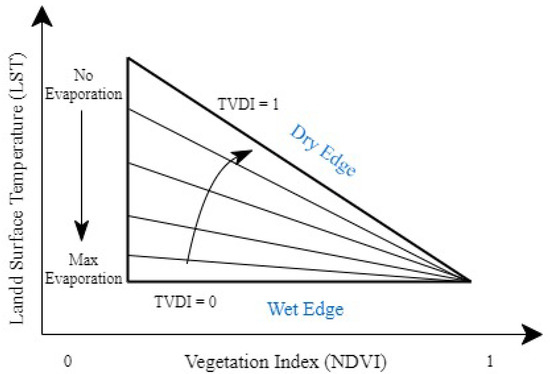
Figure 3.
Simplified triangular feature space.
Both the maximum surface temperature and the minimum surface temperature are analyzed by linear fitting equations to improve the inversion accuracy. The calculation formula is as follows:
where NDVI is the NDVI value in a given pixel, LST is the DEM corrected temperature after downscaling process in the corresponding pixel, refers to the minimum LST, and is the maximum LST in the triangle space at a given NDVI. Among the equation, is called the dry edge; is called the wet edge; , and , represent the fitting coefficient of the dry edge and wet edge equation respectively. The common NDVI range of green vegetation area is 0.2–0.8 [45]. Only the NDVI value within the range was selected. Then the corresponding TVDI value could be calculated according to the position in the LST-NDVI feature space. The TVDI value ranges from 0 to 1 and was negatively related to soil moisture.
4. Results
To investigate the performance of the DMS sharpening algorithm, the downscaled results were compared with the thermal infrared data captured by the UAS at three flight sites. TVDI calculations were then carried out using downscaled LST data, and soil moisture sampling at two flight sites was used to confirm the results.
4.1. Performance of Downscaled LST
The 10-m Sentinel-2 Vis-NIR data (Figure 4a only exhibits the RGB bands compositing image, not including NIR band) were used to sharpen the original 1-km MODIS TIR image (Figure 4b). The relationship between the Vis-NIR and LST data of coarse resolution was applied to the fine resolution Vis-NIR data with residuals to obtain the downscaled 10-m resolution LST image (Figure 4c). As shown in Figure 4, while persisting the pattern of the original MODIS LST map, the downscaled LST data also enhances the spatial features in detail based on the Sentinel-2 image. The bias is −0.075 K, and Root Mean Square Difference (RMSD) is 1.257 K between the original MODIS TIR image and the downscaled LST aggregated to 1-km resolution. Analyzing the data from a coarse resolution perspective, it is evident that DMS can build a good relationship between Vis-NIR and TIR bands across multiple satellites. Sentinel-2 provides fine-resolution Vis-NIR data with 4–5 days of revisiting time, while MODIS provides coarse-resolution LST data on a daily basis. By combining these two readily accessible satellite data, LST data with fine spatial-temporal frequencies can be generated using the downscaling method.
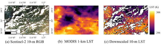
Figure 4.
Input data ((a) 10-m Sentinel-2 RGB, (b) 1-km MODIS TIR) and output data ((c) 10-m downscaling TIR) in downscaling area.
4.2. Evaluation of Downscaled LST Data with LST from UAS
To evaluate the performance of the DMS method in the study area, the downscaled LST data of each scene was compared with the thermal data from the UAS flights at three different sites (Gu Daokou, Xi Shenggou, Xi Dabei). The results were evaluated visually and quantitatively against the aggregated LST data from the UAS.
The orthophotos (Figure 5, row 1) show the surface conditions of the three flight sites. To facilitate the validation, the ultra-fine-resolution TIR images acquired by the UAS (Figure 5, row 2) were aggregated to 10-m resolution (Figure 5, row 3), which follows the pixel size of the Sentinel-2 imagery. As shown in row 4 and row 5 of Figure 5, the downscaled LST data and the original MODIS 1-km LST data were clipped to the sites’ area. Clearly, under 1 km resolution, one pixel of the MODIS LST data is much larger than the site area, making it impossible to provide adequate LST information at the field scale. By implementing the downscaling algorithm, a more detailed LST distribution was recovered, which further shows a similar pattern as the one aggregated from the UAS LST data. Compared with the maps of the original MODIS LST data, although deviation still exists between the two data sets, the downscaled data show good differentiation between high-temperature bare land and low-temperature vegetation coverage areas.
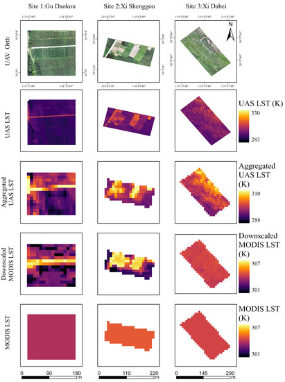
Figure 5.
Comparisons among UAS orthophotos (first row), spatial distributions of UAS LST (second row, 0.1 m), UAS aggregated LST (third row, 10 m × 10 m), downscaled LST from MODIS (fourth row 10 m × 10 m), MODIS LST (last row, 1 km × 1 km) in three flight sites (Gu Daokou, Xi Shenggou, Xi Dabei at three columns respectively).
Further analysis of the differences between the downscaled data and UAS data was done with a quantitative approach. The boxplots in Figure 6 display the range of UAS aggregated LST and DMS downscaled LST at three flight sites. Boxplots show the quartiles (the black box), median (straight red line in the box), whiskers (straight line out the box), and outliers (black dots). It is intuitively displayed that the DMS method predicts a higher median LST value than the UAS observation value in all three sites. Several factors, including atmosphere, emissivity, and the instrument’s height, can affect the performance of UAS and satellite sensors [46], which may result in the bias shown above. However, since in the following procedures, the TVDI will be calculated based on the normalized LST data, only minor influence will be introduced by the bias between the absolute value of the downscaled and UAS LST data. Moreover, the downscaled LST data is relatively concentrated (mostly in upper and lower quartiles), whereas aggregated LST data from UAS has a higher degree of dispersion. Due to the original MODIS LST data representing the average temperature over 1 area, the downscaled LST variations tend to be small, even with fine-resolution NDVI data. From the first column of Figure 5, it can be seen that the outliers in Figure 6a are mainly the LST of the road. These outliers are not the wrong value; they just represent a much higher road LST than the farmland LST that dominated the image. The UAS LST data show a wider variation and have more outlier points, suggesting that the UAS still has advantages in capturing more detailed ground information.
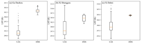
Figure 6.
Boxpltos of UAS aggregated LST and DMS downscaled LST at three flight sites.
Figure 7 shows the scatter plots comparing the aggregated LST data measured by the UAS with the downscaled LST data collected by the satellite at three flight sites. (Coefficient of Determination), RMSE (Root Mean Squared Error), and MAE (Mean Absolute Error) were computed to observe the consistency and uncertainty between downscaled LST and UAS LST. Due to the uniform and dense vegetation covering Site 1, the temperature distribution was highly concentrated, which introduced difficulties in establishing a proper correlation. The other two sites (Xi Shenggou and Xi Dabei), however, showed a relatively reliable linear relationship between the downscaled LST data and the actual UAS LST data based on the (0.74, 0.51 in two sites). The RMSE and MAE are 6.44 K, 5.94 K, and 5.72 K, 5.32 K for two sites.
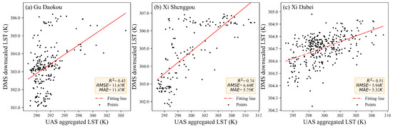
Figure 7.
Scatterplots of the UAS aggregated LST and DMS downscaled LST at three flight sites.
Compared with the UAS LST data, the DMS downscaled LST data reconstructed the spatial distribution of the LST quite well. There were still discrepancies in the obtained median values and data distributions. Due to the lack of LST validation methods for heterogeneous and across different scales, the harmonization of LST data was difficult, so the comparison was only used as a reference for downscaling LST. Nevertheless, medium correlations were still observed between the two data sets. Overall, considering the very large ratio between the original resolution and the target resolution (1 km to 10 m), the results indicate a good performance of the DMS algorithm in generating fine-resolution LST images. Even though the downscaling method cannot fully restore the LST distribution captured by the UAS, it has improved greatly compared to the satellite data. Since these satellite data are readily available, this method has high practical potential.
4.3. Calculation and Spatial Distribution of the TVDI
The DEM corrected LST is shown in Figure 8a. As introduced in Section 3, the TVDI is based on the scatterplot of the NDVI and downscaled, DEM-corrected LST of corresponding pixels. The maximum and minimum LSTs vary along with the NDVIs and can be linearly regressed to dry edge and wet edge, respectively. Figure 9 shows dry/wet edges and their fitting equations derived from density scatterplots. For this study, the fitted dry and wet edge functions are as follows:
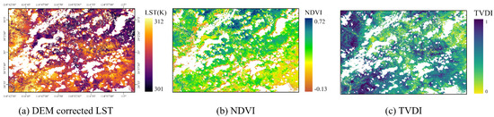
Figure 8.
Input data ((a) 10-m DEM Corrected LST, (b) 10-m NDVI) and output data ((c) 10-m TVDI) of TVDI method in downscaling area.
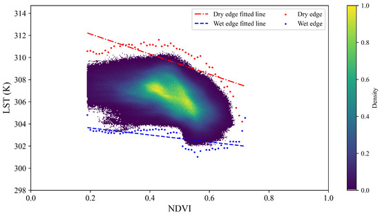
Figure 9.
Dry/wet edges and their fitting equations derived from density scatterplots of NDVI and downscaled LST.
The coefficient of determination of the corresponding dry edge is high ( > 0.55), and the of most wet edges is above 0.36.
As shown in Figure 8a–c, the downscaled, DEM-corrected LST data, the NDVI data, and the calculated TVDI data at a resolution of 10 m display similar spatial distributions across the study area. Figure 1 and Figure 8 show that in the western area of low-altitude mountains, the LST is extremely high, and the TVDI is close to 1, indicating that these regions are dry primarily due to high LST. It is likely that the sparse vegetation (low NDVI values) in the southeastern low-altitude mountainous areas mainly contributes to the low TVDI values. The low-altitude alluvial plains in the central and northeastern regions are also relatively wet, with relatively low LST, moderate NDVI, and low TVDI values. Combining the elevation map, geomorphological map, and TVDI distribution map, we found that wet areas are mainly in low-elevation alluvial plains near rivers, which often have underground aquifers and are rich in sand and gravel that can keep water.
4.4. Validation TVDI with In-Situ SM
To quantitatively validate the TVDI as an index for assessing soil moisture, in-situ soil moisture measurements were conducted at two different sites (Site 2 and Site 3). Site 1, where dense cornfields were watered, was not suitable for soil moisture sampling. Figure 10 shows the distribution of soil moisture sampling points on the UAS orthophotos and TVDI maps. Thirty-four and twenty-nine soil moisture sampling points were taken in Site 2 and Site 3, respectively. In Site 2, soil moisture varied greatly due to the heterogeneity of land cover types. The heterogeneous land cover regions can be visually observed from the UAS orthophoto. To reduce the errors and recover the overall soil moisture level for different land cover types, it was reasonable to take the mean value of the measured volumetric soil moisture under the same land cover at the 10-m Sentinel-2 grid. Thirty-four SM samples at Site 2 were divided into 12 verifying groups based on land cover boundaries (blue line). In the homogeneous land-covered Site 3, TVDI was validated against the in-situ measurements for each grid.
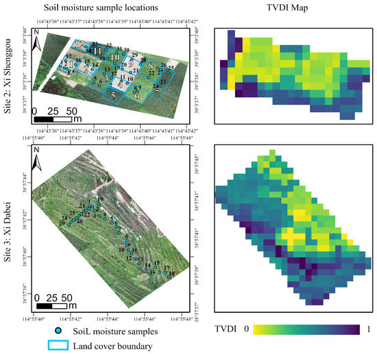
Figure 10.
The distribution of soil moisture sampling points in the UAS orthophotos (first column) and the TVDI maps (second column) in two sites.
Typically, the correlation analysis was used to assess the ability of TVDI to capture the spatial-temporal soil moisture variations [29,30]. In this study, Pearson’s correlational analysis was adopted to assess the downscaled TVDI performance. Figure 11 displays the scatter plots for the obtained TVDI data and the in-situ measured SM in the two sites, where a significant negative correlation was observed. The Pearson correlation coefficient (r) values ranged from 0.67 to 0.71, with p-value smaller than 0.05. By validating at two sites on individual days, it was suggested that the TVDI obtained through the downscaled LST data could capture the spatial variation of the SM at fine resolution. The slightly higher r at Site 2 may be attributed to the high diversity of land cover types. Furthermore, the reduction of fluctuations by averaging multiple data points also helped to make the result more reliable. At Site 3, the smaller p-value may partly be explained by the more statistics. Linear relationships exist between the TVDI and the in-situ measured SM with values ranging from 0.44 (Site 3) to 0.50 (Site 2). It is possible to use downscaled TVDI to predict the SM. Given the dry condition of the flight sites, soils with moisture greater than 15% were not involved in our study.
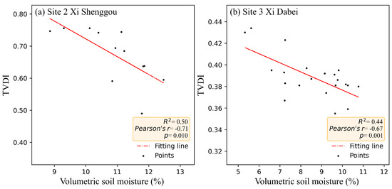
Figure 11.
Scatterplots of the soil moisture and TVDI in two flight sites.
Although many studies have proved the relationship between the soil moisture and the TVDI [12,25], this study focuses on whether TVDI, after downscaling to 10 m, can still effectively evaluate the soil moisture status. First, compared to the UAS LST data, it was verified that the downscaled satellite LST data could reflect the spatial temperature variation. Secondly, using downscaled LST data, the TVDI map still showed a reasonable SM spatial pattern over the region. The downscaled TVDI also had a good correlation with SM measurements, indicating that downscaled TVDI could reflect the condition of SM.
5. Discussion
5.1. Limitations of the DMS Algorithm
In this study, a downscaling algorithm was adopted to produce higher-resolution data sets. Generally speaking, the key point of most downscaling algorithms is to establish a statistical relationship between low-resolution and single or multiple fine-resolution data. To produce the required fine-resolution LST data, the DMS algorithm implemented by this study took the MODIS TIR data as the sharpening candidate and the fine-resolution Vis-NIR data from Sentinel-2 as the inputs. Among all the accessible bands of the Sentinel-2 data, only four Vis-NIR bands of the 10-m resolution were chosen to provide the fine-resolution information. The reason is that due to the discrepancies of the bands, a large systematic error could be introduced if multiple bands with different resolutions were adopted in the downscaling algorithm. On the other hand, to reduce the error of the correlation, it is always preferred to include as much information as possible. To further improve the results of this study, trying to incorporate other bands into the downscaling algorithm without increasing the systematic error will be a promising direction.
It is also beneficial to investigate the correlation between different variables instead of different bands. For instance, the linear relationship between the LST and the vegetation indices was studied. However, this algorithm was not suitable for this study since it averaged out the information on soil moisture, which was crucial for the LST-NDVI triangle method. In contrast, by incorporating two more bands besides the ones used in the NDVI calculation, the DMS algorithm presumably preserves the information of the soil moisture and will propagate them into the downscaled LST data.
There is an inherent limitation in applying the DMS algorithm: The specific relationship between different optical bands highly depends on the local climates, and the data acquisition time, i.e., correlations need to be established for each study area separately.
Nevertheless, it is still reliable to implement the algorithm when the data sets are spatially and temporally limited.
5.2. Differences between UAS LST and MODIS Downscaled LST
Compared to the UAS LST image, the downscaled LST data showed a similar distribution. However, discrepancies still existed. The main possible reasons are as follows:
Firstly, systematic errors could be introduced by the differences between the satellite TIR instruments, whose data were directly related to the obtained LST image, and drone thermal infrared camera sensors. A relevant study made by Combs et al. [47] compared the NDVI datasets from Sentinel-2 and the UAS, concluding that the differences are mostly due to sensor specifications and performance. It is necessary to modify LST based on the surface emissivity during retrieval. UASs were evaluated on the basis of their broadband emissivity product, while MODIS was evaluated on the basis of its emissivity product. For MODIS, an emissivity product was used, and for UAS, broadband emissivity is considered a constant for all pixels. An emissivity error can consequently lead to uncertainties in the camera performance and in the final LST retrieval [48]. In addition, the satellite TIR sensor is affected by atmospheric compounds and requires correction.
Second, the different working altitudes of the satellite and the UAS could also be one source of the systematic error. Taking advantage of its low cruising altitude, the UAS can naturally capture more pure pixels, which are relatively less smeared by adjacent pixels. It enables the UAS to better distinguish different land cover types and, at the same time to observe a wider temperature distribution. On the other hand, high-altitude satellites are more affected by the smearing of the pixels, i.e., local fluctuations originating from the small changes in the land cover tend to be mixed and averaged out. According to this, the downscaled LST data were expected to have a more concentrated distribution and to possess less information about the spatially heterogeneous. According to Panagiotis et al. [49], high homogeneity was observed in the downscaled LST data, where adjacent pixels are similar, resulting in clumped patterns and hot spots.
Thirdly, temporal consistency between the satellite data acquisition time and UAS data collection time also needs to be carefully considered. Considering the circular velocity of the satellite, with the fixed revisit time, one may assume that the satellite data were acquired at the same time in a day, especially when the study area was limited. On the other hand, a time difference always exists when collecting data at multiple sites using the UAS. This deviation in the measuring time between different data acquisition methods may result in the natural discrepancies in the measured LST distributions.
However, since that the UAS is extremely sensitive to temporal temperature fluctuations and spatial outliers, it could also lead to an unreliable representation of the overall area surface temperature.
5.3. TVDI Index Mapping SM
In this paper, the TVDI index was adopted to reflect the dry and wet conditions of the soil. Although the method is simple and easy to implement, only two independent variables are considered specifically: surface temperature and vegetation index. On the other hand, climate, vegetation cover, and soil types vary widely across regions, all of which may impact the soil conditions but instead be averaged out in the TVDI calculation. With available auxiliary information, the results could be further improved.
Another potential issue shows up when the land cover classes are not sufficiently diverse at variable levels of wetness. In this case, the LST-NDVI triangular feature space may not be successfully derived. Therefore, a certain part of the Tang River Basin was chosen as the area of interest to ensure that there were enough types of surface covers. Similar requirements also apply when collecting data with drones. To successfully acquire LST-NDVI triangles, it is required to cover as many surface types as possible, which is, however, difficult to meet. This indicates the potentially higher feasibility of SM monitoring using satellites.
Although the linear correlation between the TVDI and the SM was clearly seen in this study, there is still one caveat that the TVDI represents only relative soil moisture. Difficulties exist when trying to retrieve the absolute volumetric soil moisture due to the lack of extensive long-term in-situ monitoring SM data. However, it still has great potential when being used in environmental applications such as soil moisture monitoring and drought severity assessments. Incorporating more correction steps (such as correcting LST images) and including a wider range of SM points may improve the reliability of the results.
6. Conclusions
LST data provide vital information for remote sensing monitoring soil moisture, but the corresponding fine-resolution TIR sensor required for field-scale applications is lacking. This study aims to investigate the feasibility of using the downscaled LST data from remote sensing to monitor soil moisture via the TVDI method. A robust data mining sharpener (DMS) approach has been applied to downscale LST data, using a cubic regression tree method to establish functional relationships between the TIR and Vis-NIR bands. Due to the lack of fine-resolution TIR data for benchmarking, the downscaled LST data was evaluated using UAS observations and then applied to calculate the TVDI values. A correlational analysis was adopted between TVDI data and soil moisture in-situ measurements as a final step. The main findings and conclusions of this article are as follows:
- 1.
- The overall downscaling LST enhanced the spatial features based on the Sentinel-2 Vis-NIR bands while preserving the overall LST information of the original MODIS data. The bias was −0.075 K, and the RMSD was 1.257 K between the original MODIS TIR image and the downscaled LST aggregated to a 1-km resolution. Examined from a coarse resolution perspective, it shows that the DMS technique can build a good relationship between Vis-NIR and TIR band across multiple satellites.
- 2.
- The UAS ultra-fine resolution LST images are aggregated to the same 10-m resolution as the comparing reference of downscaled LST. Examined from a fine resolution perspective, the results showed that a more detailed LST distribution was recovered by implementing the DMS algorithm. The downscaled LST data can reflect the spatial distribution of temperature to a certain extent, though discrepancies still exist from the absolute values. DMS provides a feasible way for obtaining LST data at finer resolution.
- 3.
- Based on downscaled LST data, we obtained a reasonable TVDI distribution map. Compared with in-situ SM measurements, the downscaled TVDI could capture the spatial variations of soil moisture effectively. The TVDI derived from downscaled LST data showed a reasonable SM spatial pattern over the region, and a strong correlation with soil moisture content measurements, with Pearson’s r values, ranged from 0.67 to 0.71.
Our study demonstrates that the TVDI method based on the downscaled LST has a high potential to provide large-scale SM monitoring. However, further research is still needed to fully cover the scale gap between the satellite data and in-situ measurements. By adopting additional spatial and temporal information, the algorithm could be further validated. Moreover, by adding more factors to the downscaling algorithm, such as the cover types, or combining different sharpening methods, the systematic error can be further reduced.
Author Contributions
Conceptualization, X.M. and L.C.; methodology, L.C. and S.L.; software, L.C.; validation, L.C., X.M., S.L., S.H., H.Z. and C.X; investigation, X.M., S.L., L.C., S.H., H.Z. and C.X.; resources, X.M., P.B.-G., S.N. and H.G.; writing—original draft preparation, L.C.; writing—review and editing, X.M., S.L., S.H. and P.B.-G.; visualization, L.C.; supervision, X.M. and S.L.; project administration, X.M. and S.L.; funding acquisition, X.M. All authors have read and agreed to the published version of the manuscript.
Funding
This study was funded by the project of the National Key Research and Development Program of China (Grant Nos. 2018YFE0106500, 2022YFF0801804) and CHINA WATERSENSE (file number 8087-00002B).
Institutional Review Board Statement
Not applicable.
Informed Consent Statement
Not applicable.
Data Availability Statement
Satellite data for TVDI calculation is publicly available at the Google Earth Engine platform (https://developers.google.com/earth-engine, accessed on 25 November 2022) and is described in the main document.
Acknowledgments
We thank all the data providers.
Conflicts of Interest
The authors declare no conflict of interest.
Abbreviations
The following abbreviations are used in this manuscript:
| SM | Soil moisture |
| NDVI | Normalized difference vegetation index |
| LST | Land surface temperature |
| TVDI | Temperature vegetation dryness index |
| UAS | Unmanned aerial systems |
| TIR | Thermal infrared |
| DMS | Data mining sharpener |
References
- Seneviratne, S.I.; Corti, T.; Davin, E.L.; Hirschi, M.; Jaeger, E.B.; Lehner, I.; Orlowsky, B.; Teuling, A.J. Investigating soil moisture–climate interactions in a changing climate: A review. Earth-Sci. Rev. 2010, 99, 125–161. [Google Scholar] [CrossRef]
- Holzman, M.E.; Rivas, R.; Piccolo, M.C. Estimating soil moisture and the relationship with crop yield using surface temperature and vegetation index. Int. J. Appl. Earth Obs. Geoinf. 2014, 28, 181–192. [Google Scholar] [CrossRef]
- Brocca, L.; Moramarco, T.; Melone, F.; Wagner, W.; Hasenauer, S.; Hahn, S. Assimilation of Surface- and Root-Zone ASCAT Soil Moisture Products Into Rainfall–Runoff Modeling. IEEE Trans. Geosci. Remote Sens. 2011, 50, 2542–2555. [Google Scholar] [CrossRef]
- Cunha, A.P.M.; Alvalá, R.C.; Nobre, C.A.; Carvalho, M.A. Monitoring vegetative drought dynamics in the Brazilian semiarid region. Agric. For. Meteorol. 2015, 214–215, 494–505. [Google Scholar] [CrossRef]
- Liu, D.; Mishra, A.K.; Yu, Z.; Yang, C.; Konapala, G.; Vu, T. Performance of SMAP, AMSR-E and LAI for weekly agricultural drought forecasting over continental United States. J. Hydrol. 2017, 553, 88–104. [Google Scholar] [CrossRef]
- Western, A.W.; Blöschl, G. On the spatial scaling of soil moisture. J. Hydrol. 1999, 217, 203–224. [Google Scholar] [CrossRef]
- Dobriyal, P.; Qureshi, A.; Badola, R.; Hussain, S.A. A review of the methods available for estimating soil moisture and its implications for water resource management. J. Hydrol. 2012, 458–459, 110–117. [Google Scholar] [CrossRef]
- Sagan, V.; Maimaitijiang, M.; Sidike, P.; Maimaitiyiming, M.; Erkbol, H.; Hartling, S.; Peterson, K.T.; Peterson, J.; Burken, J.; Fritschi, F. UAV/Satellite Multiscale Data Fusion for Crop Monitoring and Early Stress Detection. Int. Arch. Photogramm. Remote Sens. Spat. Inf. Sci. 2019, XLII-2/W13, 715–722. [Google Scholar] [CrossRef]
- Verstraeten, W.W.; Veroustraete, F.; Feyen, J. Assessment of Evapotranspiration and Soil Moisture Content Across Different Scales of Observation. Sensors 2008, 8, 70–117. [Google Scholar] [CrossRef]
- Garrison, J.L.; Shah, R.; Kim, S.; Piepmeier, J.; Vega, M.A.; Spencer, D.A.; Banting, R.; Raymond, J.C.; Nold, B.; Larsen, K.; et al. Analyses Supporting Snoopi: A P-Band Reflectometry Demonstration 2020. In Proceedings of the IGARSS 2020—2020 IEEE International Geoscience and Remote Sensing Symposium, Waikoloa, HI, USA, 26 September–2 October 2020; pp. 3349–3352. [Google Scholar] [CrossRef]
- Dai, E.; Venkitasubramony, A.; Gasiewski, A.; Stachura, M.; Elston, J. High Spatial Soil Moisture Mapping Using Small Unmanned Aerial System. In Proceedings of the IGARSS 2018—2018 IEEE International Geoscience and Remote Sensing Symposium, Valencia, Spain, 22–27 July 2018; pp. 6496–6499. [Google Scholar] [CrossRef]
- Petropoulos, G.P.; Ireland, G.; Barrett, B. Surface soil moisture retrievals from remote sensing: Current status, products & future trends. Phys. Chem. Earth Parts A/B/C 2015, 83–84, 36–56. [Google Scholar] [CrossRef]
- Escorihuela, M.J.; Quintana-Seguí, P. Comparison of remote sensing and simulated soil moisture datasets in Mediterranean landscapes. Remote Sens. Environ. 2016, 180, 99–114. [Google Scholar] [CrossRef]
- Naeimi, V.; Bartalis, Z.; Wagner, W. ASCAT Soil Moisture: An Assessment of the Data Quality and Consistency with the ERS Scatterometer Heritage. J. Hydrometeorol. 2009, 10, 555–563. [Google Scholar] [CrossRef]
- Entekhabi, D.; Njoku, E.; O’Neill, P.; Kellogg, K.H.; Crow, W.; Edelstein, W.N.; Entin, J.; Goodman, S.; Jackson, T.; Johnson, J.; et al. The Soil Moisture Active and Passive (SMAP) mission. Proc. IEEE 2010, 98, 704–716. [Google Scholar] [CrossRef]
- Dorigo, W.A.; Gruber, A.; De Jeu, R.A.M.; Wagner, W.; Stacke, T.; Loew, A.; Albergel, C.; Brocca, L.; Chung, D.; Parinussa, R.M.; et al. Evaluation of the ESA CCI soil moisture product using ground-based observations. Remote Sens. Environ. 2015, 162, 380–395. [Google Scholar] [CrossRef]
- Njoku, E.G.; Wilson, W.J.; Yueh, S.H.; Dinardo, S.J.; Li, F.K.; Jackson, T.J.; Lakshmi, V.; Bolten, J. Observations of soil moisture using a passive and active low-frequency microwave airborne sensor during SGP99. IEEE Trans. Geosci. Remote Sens. 2002, 40, 2659–2673. [Google Scholar] [CrossRef]
- Kaleita, A.; Tian, L.F.; Hirschi, M. Relationship between soil moisture content and soil surface reflectance. Trans. ASAE 2005, 48, 1979–1986. [Google Scholar] [CrossRef]
- Weidong, L.; Baret, F.; Xingfa, G.; Qingxi, T.; Lanfen, Z.; Bing, Z. Relating soil surface moisture to reflectance. Remote Sens. Environ. 2002, 81, 238–246. [Google Scholar] [CrossRef]
- Gao, Z.; Xu, X.; Wang, J.; Yang, H.; Huang, W.; Feng, H. A method of estimating soil moisture based on the linear decomposition of mixture pixels. Math. Comput. Model. 2013, 58, 606–613. [Google Scholar] [CrossRef]
- Wang, L.; Qu, J. NMDI: A normalized multi-band drought index for monitoring soil and vegetation moisture with satellite remote sensing. Geophys. Res. Lett. 2007, 34. [Google Scholar] [CrossRef]
- Casamitjana, M.; Torres-Madroñero, M.C.; Bernal-Riobo, J.; Varga, D. Soil Moisture Analysis by Means of Multispectral Images According to Land Use and Spatial Resolution on Andosols in the Colombian Andes. Appl. Sci. 2020, 10, 5540. [Google Scholar] [CrossRef]
- Verstraeten, W.W.; Veroustraete, F.; van der Sande, C.J.; Grootaers, I.; Feyen, J. Soil moisture retrieval using thermal inertia, determined with visible and thermal spaceborne data, validated for European forests. Remote Sens. Environ. 2006, 101, 299–314. [Google Scholar] [CrossRef]
- Matsushima, D.; Kimura, R.; Shinoda, M. Soil Moisture Estimation Using Thermal Inertia: Potential and Sensitivity to Data Conditions. J. Hydrometeorol. 2012, 13, 638–648. [Google Scholar] [CrossRef]
- Toby, C. An Overview of the “Triangle Method” for Estimating Surface Evapotranspiration and Soil Moisture from Satellite Imagery. Sensors 2007, 7, 1612. [Google Scholar] [CrossRef]
- Sadeghi, M.; Babaeian, E.; Tuller, M.; Jones, S.B. The optical trapezoid model: A novel approach to remote sensing of soil moisture applied to Sentinel-2 and Landsat-8 observations. Remote Sens. Environ. 2017, 198, 52–68. [Google Scholar] [CrossRef]
- Sandholt, I.; Rasmussen, K.; Andersen, J. A simple interpretation of the surface temperature/vegetation index space for assessment of surface moisture status. Remote Sens. Environ. 2002, 79, 213–224. [Google Scholar] [CrossRef]
- Mallick, K.; Bhattacharya, B.K.; Patel, N.K. Estimating volumetric surface moisture content for cropped soils using a soil wetness index based on surface temperature and NDVI. Agric. For. Meteorol. 2009, 149, 1327–1342. [Google Scholar] [CrossRef]
- Zhu, W.; Jia, S.; Lv, A. A time domain solution of the Modified Temperature Vegetation Dryness Index (MTVDI) for continuous soil moisture monitoring. Remote Sens. Environ. 2017, 200, 1–17. [Google Scholar] [CrossRef]
- Sun, L.; Sun, R.; Li, X.; Liang, S.; Zhang, R. Monitoring surface soil moisture status based on remotely sensed surface temperature and vegetation index information. Agric. For. Meteorol. 2012, 166–167, 175–187. [Google Scholar] [CrossRef]
- Zhan, W.; Chen, Y.; Zhou, J.; Wang, J.; Liu, W.; Voogt, J.; Zhu, X.; Quan, J.; Li, J. Disaggregation of remotely sensed land surface temperature: Literature survey, taxonomy, issues, and caveats. Remote Sens. Environ. 2013, 131, 119–139. [Google Scholar] [CrossRef]
- Bai, L.; Long, D.; Yan, L. Estimation of Surface Soil Moisture With Downscaled Land Surface Temperatures Using a Data Fusion Approach for Heterogeneous Agricultural Land. Water Resour. Res. 2019, 55, 1105–1128. [Google Scholar] [CrossRef]
- Kustas, W.P.; Norman, J.M.; Anderson, M.C.; French, A.N. Estimating subpixel surface temperatures and energy fluxes from the vegetation index–radiometric temperature relationship. Remote Sens. Environ. 2003, 85, 429–440. [Google Scholar] [CrossRef]
- Gao, F.; Masek, J.; Schwaller, M.; Hall, F. On the blending of the Landsat and MODIS surface reflectance: Predicting daily Landsat surface reflectance. IEEE Trans. Geosci. Remote Sens. 2006, 44, 2207–2218. [Google Scholar] [CrossRef]
- Agam, N.; Kustas, W.P.; Anderson, M.C.; Li, F.; Neale, C.M.U. A vegetation index based technique for spatial sharpening of thermal imagery. Remote Sens. Environ. 2007, 107, 545–558. [Google Scholar] [CrossRef]
- Yang, G.; Pu, R.; Huang, W.; Wang, J.; Zhao, C. A Novel Method to Estimate Subpixel Temperature by Fusing Solar-Reflective and Thermal-Infrared Remote-Sensing Data With an Artificial Neural Network. IEEE Trans. Geosci. Remote Sens. 2009, 48, 2170–2178. [Google Scholar] [CrossRef]
- Gao, F.; Kustas, W.P.; Anderson, M.C. A Data Mining Approach for Sharpening Thermal Satellite Imagery over Land. Remote Sens. 2012, 4, 3287–3319. [Google Scholar] [CrossRef]
- Bindhu, V.M.; Narasimhan, B.; Sudheer, K. Development and verification of a non-linear disaggregation method (NL-DisTrad) to downscale MODIS land surface temperature to the spatial scale of Landsat thermal data to estimate evapotranspiration. Remote Sens. Environ. 2013, 135, 118–129. [Google Scholar] [CrossRef]
- Sánchez, J.M.; Galve, J.M.; González-Piqueras, J.; López-Urrea, R.; Niclòs, R.; Calera, A. Monitoring 10-m LST from the Combination MODIS/Sentinel-2, Validation in a High Contrast Semi-Arid Agroecosystem. Remote Sens. 2020, 12, 1453. [Google Scholar] [CrossRef]
- Guzinski, R.; Nieto, H. Evaluating the feasibility of using Sentinel-2 and Sentinel-3 satellites for high-resolution evapotranspiration estimations. Remote Sens. Environ. 2019, 221, 157–172. [Google Scholar] [CrossRef]
- Xiang, T.Z.; Xia, G.S.; Zhang, L. Mini-Unmanned Aerial Vehicle-Based Remote Sensing: Techniques, applications, and prospects. IEEE Geosci. Remote Sens. Mag. 2019, 7, 29–63. [Google Scholar] [CrossRef]
- Oliver, W.; Bryan, M.; Jeffrey, M.; Michel, B.; Laura, L. Sub-metre mapping of surface soil moisture in proglacial valleys of the tropical Andes using a multispectral unmanned aerial vehicle. Remote Sens. Environ. 2019, 222, 104–118. [Google Scholar] [CrossRef]
- Wang, J. 1:1,000,000 Geomrphological Map of Beijing, Tianjin and Hebei Region. Available online: https://data.casearth.cn/sdo/detail/5c19a5670600cf2a3c557b37 (accessed on 13 December 2022).
- Zhao, J.; Zhang, X.; Liao, C.; Bao, H. TVDI based Soil Moisture Retrieval from Remotely Sensed Data over Large Arid Areasin. Remote Sens. Technol. Appl. 2011, 26, 742–750. (In Chinese) [Google Scholar]
- Lowe, A.; Harrison, N.; French, A.P. Hyperspectral image analysis techniques for the detection and classification of the early onset of plant disease and stress. Plant Methods 2017, 13, 80. [Google Scholar] [CrossRef] [PubMed]
- Awais, M.; Li, W.; Hussain, S.; Cheema, M.J.M.; Li, W.; Song, R.; Liu, C. Comparative Evaluation of Land Surface Temperature Images from Unmanned Aerial Vehicle and Satellite Observation for Agricultural Areas Using In Situ Data. Agriculture 2022, 12, 184. [Google Scholar] [CrossRef]
- Combs, T.P.; Didan, K.; Dierig, D.; Jarchow, C.J.; Barreto-Muñoz, A. Estimating Productivity Measures in Guayule Using UAS Imagery and Sentinel-2 Satellite Data. Remote Sens. 2022, 14, 2867. [Google Scholar] [CrossRef]
- García-Santos, V.; Cuxart, J.; Jiménez, M.A.; Martínez-Villagrasa, D.; Simó, G.; Picos, R.; Caselles, V. Study of Temperature Heterogeneities at Sub-Kilometric Scales and Influence on Surface–Atmosphere Energy Interactions. IEEE Trans. Geosci. Remote Sens. 2019, 57, 640–654. [Google Scholar] [CrossRef]
- Sismanidis, P.; Keramitsoglou, I.; Kiranoudis, C.T.; Bechtel, B. Assessing the Capability of a Downscaled Urban Land Surface Temperature Time Series to Reproduce the Spatiotemporal Features of the Original Data. Remote Sens. 2016, 8, 274. [Google Scholar] [CrossRef]


Disclaimer/Publisher’s Note: The statements, opinions and data contained in all publications are solely those of the individual author(s) and contributor(s) and not of MDPI and/or the editor(s). MDPI and/or the editor(s) disclaim responsibility for any injury to people or property resulting from any ideas, methods, instructions or products referred to in the content. |
© 2023 by the authors. Licensee MDPI, Basel, Switzerland. This article is an open access article distributed under the terms and conditions of the Creative Commons Attribution (CC BY) license (https://creativecommons.org/licenses/by/4.0/).