Abstract
Classification algorithms integrated with convolutional neural networks (CNN) display high accuracies in synthetic aperture radar (SAR) image classification. However, their consideration of spatial information is not comprehensive and effective, which causes poor performance in edges and complex regions. This paper proposes a Markov random field (MRF)-based algorithm for SAR image classification which fully considers the spatial constraints between superpixel regions. Firstly, the initialization of region labels is obtained by the CNN. Secondly, a probability field is constructed to improve the distribution of spatial relationships between adjacent superpixels. Thirdly, a novel region-level MRF is employed to classify the superpixels, which combines the intensity field and probability field in one framework. In our algorithm, the generation of superpixels reduces the misclassification at the pixel level, and region-level misclassification is rectified by the improvement of spatial description. Experimental results on simulated and real SAR images confirm the efficacy of the proposed algorithm for classification.
1. Introduction
With the development of space science, synthetic aperture radar (SAR) technology has been widely used in natural disaster monitoring, terrain interpretation, agricultural detection, and other applications for Earth observation. Meanwhile, SAR imaging has imaging superiority over optical imaging due to its capability of acquiring high-spatial-resolution images in all-weather and all-time scenarios [1]. However, the performance of SAR images is always suppressed by speckle noise pollution, which is generated by the backward scattering of coherent electromagnetic waves. As a kind of multiplicative noise, speckle noise causes the distortion of pixel values in a wild region, which creates a series of huge challenges for SAR image processing [2].
SAR image classification is the essential technique to deal with image processing and is mainly used in recognizing and detecting topographical objects in SAR images. As a matter of fact, the purpose of image classification is to divide the image into a certain number of classes with similar features and group the purposeful parts to promote subsequent manipulation. In recent years, Markov random fields (MRF) have been widely used in both optical images and SAR images [3,4]. Unsupervised methods based on MRFs consider both the relations of features and the context of spatial information, which leads to suppressing speckle noise efficiently. An MRF obtains the results of image classification through an optimizing energy function in the Bayesian framework. Deng et al. [5] propose an anisotropic circular Gaussian MRF (ACG-MRF) for image classification, and then Wu et al. [6] improve the MRF from pixel-level to region-level by introducing Wishart distance. Li et al. [7] design a Gaussian mixture model MRF (GMM-MRF) to consider the relationships between spatial information and contextual information, and then Song et al. [8] build a mixture WGΓ-MRF (MWGΓ-MRF) to improve the surveying of textural information. Though MRF-based models have accomplished a series of successes on contextual constraints, they are still subject to a lack of prior knowledge and expert experience. Furthermore, only the low-level features are used in these unsupervised methods, which limits the accuracy of the algorithms.
Based on the multifarious mentality of designing for classifiers, there are two main categories in supervised SAR image classification, which are artificial feature extraction methods and deep learning methods [9]. The key idea of artificial feature extraction is to extract certain kinds of image features and the selection of classifiers. Primarily in the aspect of hand-crafted feature extraction, the intensity of images and the texture information are common characteristics used in reprocessing. While in classification algorithms, separate classifiers for SAR images have been proposed, such as support vector machine (SVM) [10], random forest (RF) [11], and artificial neural network (ANN) methods [12]. Although the above methods achieve a certain degree of classification accuracy and complete description of image features at a low level or middle level, the results still suffered from speckle noise and resulted in unstable robustness in different regions.
Deep learning algorithms can extract discriminative features automatically and require strong robustness against speckle noise; especially, convolutional neural networks (CNN) have gained widespread acceptance in remote sensing applications [13]. In recent years, a succession of CNN-based models have been used to classify SAR images. Zhou et al. [14] first introduced a CNN method for SAR image classification and achieved better classification accuracy than traditional artificially supervised methods, and then Wang et al. [15] proposed a multiple CNN (MP-CNN) to fuse intensity and edge information for SAR image classification. The input of a CNN is 2-D image patches which guarantee the constraints of contextual information at the pixel level [16]. However, the process of extracting characters shatters the inherent construction of the feature map in regions [17].
To maintain the inherent construction of the feature map in regions, a novel SAR image classification method using Markov random fields with deep learning is proposed in this paper. Subregions of the image are generated by the SLIC superpixels algorithm, and corresponding labels are traded off by the CNN with an internal voting strategy. The characters extracted by the CNN are introduced to enhance the description of the intensity of regions and complement the binary contextual relevance between regions. By minimizing the energy function of the proposed method, the results of the classification can be obtained. Experiments have been conducted on simulated and real SAR images to evaluate the performance of the proposed algorithm. The experimental results demonstrate that the proposed algorithm outperforms the other CNN-based region-level SAR image classification algorithms.
2. Materials and Methods
The flowchart of the proposed approach is shown in Figure 1. The motivation of the proposed method is to research the complex spatial relationships of different characters. Firstly, the pixel-level category confidence-degree features are extracted by the CNN [18], and superpixels are generated by the SLIC algorithm. The construction of the region adjacency graph (RAG) and the voting strategy accomplish the feature extraction at the region level. Subsequently, all characters are introduced into the proposed region-level MRF, and the final classification results are calculated by minimizing the total energy function.
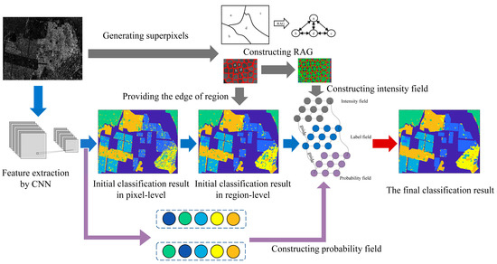
Figure 1.
Flowchart of the proposed approach. a, b, c and d are the four adjacent superpixel regions connecting based on the rule of shared boundaries. The grey arrow describes the process of constructing intensity field; the blue arrow describes the process of constructing label field; the purple arrow describes the process of constructing probability field.
2.1. Superpixel Construction
Superpixel construction is used to classify regions in the proposed method A superpixel is a subregion in an image composed of a series of adjacent pixels with similar features such as color, intensity, and textures. Compared with pixel-level segmentation algorithms, superpixels retain efficient spatial structure information for further image processing and generally reserve the boundary information. In this paper, the simple linear iterative clustering (SLIC) algorithm [19] is used to generate superpixels. The SLIC algorithm converges homogeneous spatial pixels into the same class by adaptive k-means clustering. As the most common method in regional segmentation, the SLIC algorithm owns superior performance with simple implementation, and it is meanwhile resistant to speckle noise due to considering regional consistency.
In the SLIC algorithm, the value of every superpixel is obtained by calculating the mean intensity of all pixels in each region. For better facilitating the subsequent operations, the region adjacency graph (RAG) is introduced to represent the correlations between regions [20]. The rule of connection is based on shared boundaries between regions. Figure 2 shows an example of an RAG for superpixels; the nodes denote the values of the superpixels, and the edges describe the pairwise spatial information.
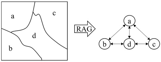
Figure 2.
Illustration of an RAG.
2.2. Initialization by Convolutional Neural Network
The convolutional neural network (CNN) is the most common tool in supervised image processing, and a traditional CNN in classification is structured as shown in Figure 3. The convolution layer can be regarded as a kind of filter to output various features from input patches, and the feature maps are constructed by iterating through all positions. The main work of the pooling layer is subsampling the feature maps to resist overfitting and increase robustness for the whole design. The fully connected layer reshapes the feature maps from two-dimensional to one-dimensional; meanwhile, the softmax layer outputs the classification results.
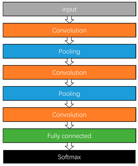
Figure 3.
The structure of a convolutional neural network.
In the softmax layer, the network outputs the pixel-level category labels and corresponding probability distribution. The probability that a pixel corresponds to different labels is listed, and the total probability for each pixel is equal to 1. The pixel-level category labels are used to generate the label field for superpixels, and the probability distribution is regarded as a deep feature to construct the probability field in the MRF.
The criterion of superpixel segmentation is clustering the spatial adjacent pixels with the same features, so the category of a superpixel region should be consistent among most pixels. Because the output of the CNN only provides pixel-wise labels, a region-based majority voting strategy is necessary for initializing RAG labels. Assume there are M pixels in superpixel r and the category of each pixel is received by the CNN, through counting the histograms of the label distribution in the region, the majority voting result will be selected as the initial category of r. The superpixel probability distribution is calculated by the joint probability of the corresponding pixels.
2.3. Region-Level Markov Random Fields
The image classification problem can be formulated as a maximum a posteriori (MAP) estimate in the manner of the Bayesian framework.
The traditional MRF model bears a sharply growing computation cost as the size of the image increases, and meanwhile, the block-level texture information fails to be completely extracted in a pixel-based framework [21]. Based on the idea of solving the above problems, a region-level MRF model is constructed to improve algorithm capacity. Compared with pixel-based MRF model, the region-level MRF model has three main advantages. Firstly, dealing with an image in region-level patterns could effectively reduce the complexity of the algorithm due to the declining number of factors in the label field. Secondly, the latent semantic information could be reflected, including the oversegmented regions [22]. Thirdly, the process of generating regions suppresses the influence of oversegmentation, and some of the pixel-level misclassification is smoothed out by regions. Generally, dealing with an image in regions can efficiently parse the structure of the topology and contextual information.
In the superpixel-based region-level MRF model for SAR image classification, the spatial context model describes the interactions between continuous superpixels, and the feature model expresses the intensity distribution for each superpixel. The feature model for an SAR image is often calculated as Gaussian distribution, and the energy function is written as:
and are the mean and variance of the intensity distribution at the class , and is the sets of superpixels which belong to class . represents all the regions in the input SAR image. Assuming two adjacent superpixels and , the energy function of the spatial context model is as follows:
expresses the label of expresses the interactions for two regions, denotes the set of all cliques in the SAR input image, and is a potential parameter to balance the contributions between the feature model and spatial context model. The MRF energy function of intensity field is integrated as:
2.4. Construction of Probability Field
It should be mentioned that the traditional superpixel-based region-level MRF model only considers the intensity characteristics, and the label field is guided by the circulation of the energy function. The Gaussian distribution is simple to calculate but rough for multiplicative noise, and punishment between adjacent superpixels is rude and unfair. In this paper, a probability field is constructed to jointly guide the label field and improve the classification accuracy. The probability field is based on the probability output of the CNN. By calculating the average probability of corresponding pixels in the same set, the superpixel probability distribution is obtained.
In accordance with the manner of the MRF model based on the intensity field, the energy function for the probability field has two parts as well. In the unary part, it quantifies the possibilities for a superpixel in each class, and the energy function can be defined as:
is the total number of pixels within the superpixel , is a random pixel in the superpixel , is the total superpixels in the input SAR image, and is the probability of the pixel belong to . calculates the confidence that the superpixels belong to their labels. Similar to the purpose of the spatial context model, the binary part is used to describe the relationship between regions. The energy function is represented as:
is the inner product between the superpixels and . is the total probability distribution for superpixel and is written as:
where is the probability distribution for the superpixel at each label, and is the total number of categories. The inner product can be computed by relying on the construction of the softmax layer in the CNN and manifests a positive correlation to similitude for adjacent superpixels. To be specific, the value of is increased when the regions are similar to each other. is the balance coefficient and agrees with the initialization in the intensity field. The energy function for the probability field is as follows:
We can obtain the total RMRF energy function for the two fields, which is shown below:
The motivation of constructing the probability field is to remedy the insufficiency of MRF model while considering the superpixel probability distribution from the CNN as the deep-level character information to be operated on in the framework of the probability field. The unary part gives the specific quantified value of which category the region belongs to, and the binary part shows the spatial context relations for superpixels. The traditional region-level MRF model gives a polarized strategy for neighborhood relationships, in which the energy function equals 1 if the regions have the same label and settles to 0 when they have different labels. The binary part of the probability field renders the strategy kindly and continuous. When the labels for adjacent regions are different, the energy function outputs a measured value to judge how different they are. When the labels are the same, the energy function also gives a detailed measurement for the similarity index.
The initial RAG label is generated by the CNN, and updating the label field is performed by minimizing the energy functions of both the intensity field and probability field. The simulated annealing (SA) algorithm is used to acquire the final classification results.
3. Experimental Study
In this section, experiments with synthetic SAR images and real SAR images are presented to evaluate the validity of the proposed classification method. The comparison methods are separately chosen from pixel-level and region-level techniques. CNN and CNN-MRF [23] are the pixel-level methods to examine the basis of the proposed method. The CNN + superpixel algorithm (CNN-SP) [24] and the region category confidence-degree-based Markov random field (RCC-MRF) method [25] are the region-level methods to verify the performance of the probability field. Firstly, the accuracy of the proposed method is explored using one synthetic SAR image and two real SAR images. Secondly, the capacity of each algorithm is determined using a TerraSAR image with a large size and high resolution. Thirdly, the robustness of each algorithm is considered by controlling the number of superpixels.
3.1. Experimental Datasets
Four SAR datasets are employed to evaluate the performance of the proposed method. The datasets consist of one synthetic SAR image, two real SAR images, and one TerraSAR image. The synthetic SAR image is always used to roughly verify the capability of classification of each algorithm; it contains eight categories with a size of 486 × 486. San Francisco Bay (SF-Bay) and the Flevoland images are the most common datasets for SAR image classification, and both were captured by the Radarsat-2 satellite, which satisfies the resolution requirement of 10 m. Both SF-Bay and Flevoland contain five categories. Lillestroem is a large and high-resolution image acquired by the TerraSAR-X satellite, and the related information of the real image datasets [26,27] is shown in Table 1.

Table 1.
Geographic information of real images.
The experiment images and corresponding ground truth are shown in Figure 4. A description of the categories for each image is introduced in the following experimental section.
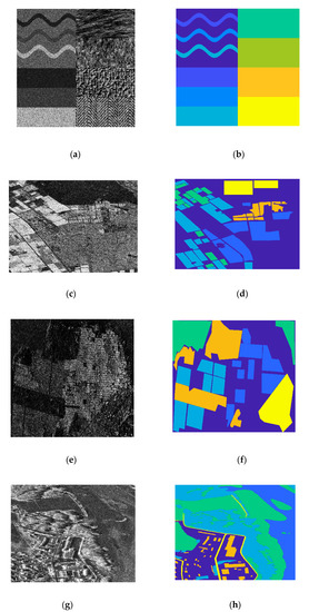
Figure 4.
SAR images and the corresponding ground truth. (a) The synthetic SAR image. (b) Ground truth for the synthetic SAR image. (c) The Flevoland image. (d) Ground truth for the Flevoland image. (e) The SF-Bay image. (f) Ground truth for the SF-Bay image. (g) The Lillestroem image. (h) Ground truth for the Lillestroem image.
3.2. Experimental Setup and Evaluation Criteria
To maintain the fairness of the experimental environment, the setup for the CNN references the design in RCC-MRF and the corresponding parameters listed in Table 2. In the CNN training process, the input image patch is set as 27 × 27, 1000 pixels in each image are randomly chosen as training samples, and others are stored to evaluate the performance of the CNN. The superpixels in each image also settle at the same number as in RCC-MRF. There are 3000 superpixels in the synthetic SAR image, and 9000 superpixels each in the SF-Bay image, Flevoland image, and Lillestroem image. The overall accuracy (OA) and kappa coefficient () are used to evaluate the classification results.

Table 2.
The parameters for the CNN.
3.3. Performance Analysis on Synthetic SAR Image
The synthetic SAR image has eight categories, having four curved boundary areas on the upper left and four textured areas on the right side. A non-linear boundary will cause incorrect positioning, and complex textures will cause misclassification, both leading to increased difficulty of classification accuracy.
The accuracies of the five methods on the synthetic SAR image are shown in Table 3. The proposed method obtains the best classification results, i.e., 95.12% in OA and 94.73% in . The OA of RCC-MRF is 93.60% and the OA of CNN-SP is 93.39%. CNN obtains the lowest value of OA, which is 90.74%.

Table 3.
Accuracies of classification on synthetic SAR image.
The classification results are shown in Figure 5. In the area with complex texture information, the differences in the same class become large, and differences between adjacent classes become small, which caused much misclassification. CNN classification, regarding results in the right half of the synthetic image, not only misjudges the boundary but also generates pixel-level misclassifications. For the proposed method, the texture information can be captured through the structure of superpixels, so it shows internal smooth and regular edge results on the textured area. The curved boundary areas on the upper left are long and narrow, and superpixels generated by SLIC do not quite fit at the edge. The oversegmentation of superpixels and speckle noise cause the region-level misclassification from class 1 to 4. For the adjacent classes 6 and 7 in CNN-MRF, due to the degree of texture similarity, the differences in the same class become large, and differences between adjacent classes become small, which causes much misclassification. The proposed method performs well in terms of regional consistency, and the initial misclassification is smoothed by the structure of the superpixels.
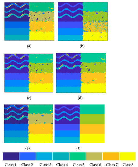
Figure 5.
The classification results on the synthetic SAR image. (a) CNN. (b) CNN-MRF. (c) CNN-SP. (d) RCC-MRF. (e) Proposed method. (f) Ground truth.
3.4. Performance Analysis on Flevoland Image
The Flevoland image is a real dataset with five categories: Forest, Farmland 1, Farmland2, Urban, and Water. To further examine the performance of the proposed method, the proposed method with 4000 superpixels will be added for real SAR image classification comparison.
The accuracies of the algorithms on the Flevoland image are listed in Table 4. The proposed method outperforms the other algorithms and obtains an OA of 89.77% and a of 86.03%. The OA of RCC-MRF is quite close to that of the proposed method at 89.44%. CNN-SP and CNN-MRF receive results of 88.90% and 88.55% respectively. Unsurprisingly, CNN has the lowest value of OA, which is 85.52%.

Table 4.
Accuracies of classification on Flevoland image.
The classification result maps for all algorithms are shown in Figure 6. Through generating superpixels, a large number of pixel-level misclassifications are smoothed out with high efficiency in the class Forest. In the class Urban, due to the complexity of the texture information, a pixel-level algorithm cannot recognize the terrains clearly, as shown in Figure 6a,b. Meanwhile in Figure 6e, establishing spatial context information between adjacent areas rectifies the region-level misclassification and shows better performance and accuracy than RCC-MRF. It should be mentioned that some region-level misclassifications increased regarding which class is labeled as Farmland 2. These inaccuracies are caused by the structure of superpixels and the poor prior knowledge from CNN with the class accuracy of 35.81%. As a result, all region-level algorithms suffer terrible classification results. Compared with CNN-SP and RCC-MRF, the proposed method still obtains a higher accuracy in Farmland 2 due to the improvement from the probability field.
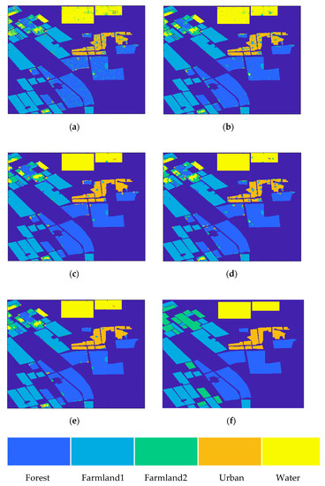
Figure 6.
The classification results on the Flevoland image. (a) CNN. (b) CNN-MRF. (c) CNN-SP. (d) RCC-MRF. (e) Proposed method. (f) Ground truth.
3.5. Performance Analysis on San Francisco Bay Image
The real dataset SF-Bay image is used to evaluate the performance of the algorithms with regard to five categories, which are Build-up 1, Build-up 2, Build-up 3, Water, and Vegetation.
The assessments of the accuracies of the five designed algorithms on the SF-Bay image are shown in Table 5. The OA of the proposed method has the highest value with a rate of 87.69%. The classification performance of RCC-MRF is better than those of the pixel-level algorithms and CNN-SP.

Table 5.
Accuracies of classification on SF-Bay image.
The classification result maps for all explored algorithms are shown in Figure 7. In Figure 7a,b, the distribution of misclassifications scatters in each category with the level of the pixel, and regions of Build-up 1, Build-up 2, and Build-up 3 suffer the majority of the inaccuracies. From Figure 7c–e, it can be seen that region-level smoothing improves the performance of the results map, and plenty of pixel-level errors vanished. Especially in the category Build-up 3 at the bottom-right corner, the proposed method reaches the highest classification accuracy with a superiority of 8.62% over RCC-MRF, which proves the outperformance of the probability field.
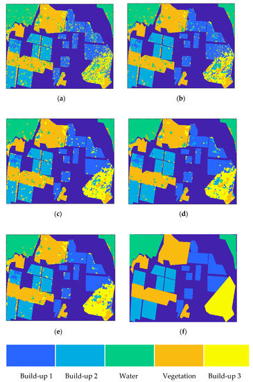
Figure 7.
The classification results on the SF-Bay image. (a) CNN. (b) CNN-MRF. (c) CNN-SP. (d) RCC-MRF. (e) Proposed method. (f) Ground truth.
3.6. Performance Analysis on Lillestroem Image
The Lillestroem image is a real dataset captured by the TerraSAR-X satellite and has five categories: River, Forest, Grassland, Building, and Road. Compared with the Flevoland and SF-Bay images, the Lillestroem image has two main characteristics. Firstly, the Lillestroem image is quite large, with a size of 3580 × 2250, and its resolution is higher than those of the Radasat-2 datasets, which created a certain challenge for the algorithms. Secondly, the terrains of Building and Road are narrow and slender, which could cause failures of superpixel segmentation.
The classification results on the Lillestroem image are listed in Table 6. The proposed method achieves the highest accuracy among the explored algorithms. In the categories of River, Forest, and Grassland, the performance of the proposed method is superior to those of the others. Meanwhile, in the category of Building, the proposed method fails to improve the accuracy, and it even becomes worse in the region of Road. The invalidation of classification is caused by two aspects: the initialization from CNN is ineffective (accuracy of CNN in Building is 22.02%, in Road is 4.82%), and the shape of the superpixels is not suitable for narrow landcover. From the classification result map of RCC-MRF, the label of Building spread to other regions, which indicates that the improvement of the result is based on overdetection, which sacrifices the accuracies of other regions. Though the proposed method fails to reach the highest accuracy in the class of Building, the corresponding label stays at the bottom right corner, which indicates that overdetection does not occur. In addition, there are certain numbers of region-level misclassifications that appear in RCC-MRF, which caused it to have the worst performance in the class of Forest. From the classification results of the proposed method, some advantages are visible to the naked eye: intra-region classification remains consistent, and boundaries between regions are relatively smooth.

Table 6.
Accuracies of classification on Lillestroem image.
The classification result maps are shown in Figure 8. In Figure 8d, RCC-MRF exhibits much region-level misclassification, especially in the category Forest. Focusing on the same field of view in Figure 8e, region-level mistakes are suppressed by the proposed method, and edges between categories become distinct to some degree.
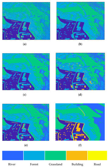
Figure 8.
The classification results on the Lillestroem image. (a) CNN. (b) CNN-MRF. (c) CNN-SP. (d) RCC-MRF. (e) Proposed method. (f) Ground truth.
3.7. Demonstrating the Effect of the Probability Field
The RCC-MRF method generates an RCC term to complement the distribution of the Gaussian mixture model. The properties of the vector form drop, and there is a lack of consideration of the correlations between adjacent regions. To further verify the capacity of the proposed method, comparisons between RCC-MRF and the proposed method are considered by increasing superpixels from 2000 to 30,000 sets. The comparison results on the SF-Bay image for the two algorithms are shown in Figure 9. Both RCC-MRF and the proposed method reach their highest OA at 9000 superpixels. With the increase of superpixels, the accuracy of RCC-MRF goes down sharply; meanwhile, the change in the proposed method is gentle and robust. The main computation cost for RCC-MRF and the proposed method lies in the superpixel generation process. When the number of superpixels is not suitable, the accuracy of segmentation will decline, which causes errors of classification to increase. RCC-MRF is more sensitive to the number of superpixels, so the right decision for selecting numbers requires repeated testing. However, the proposed method has a certain robustness regarding the number of superpixels, and it would be easy to balance the computation cost and classification accuracy.
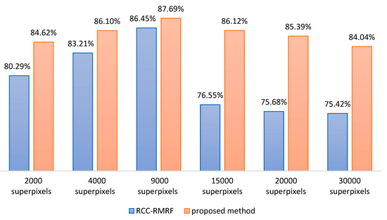
Figure 9.
The classification results of RCC-MRF and the proposed method on the SF-Bay image.
4. Conclusions
In this paper, a novel classification method using Markov random fields with deep learning is proposed for SAR images. In this method, a probability field based on neural network is proposed to describe the relationships between regions. By constructing binary and unary parts based on probabilities, the contextual information is fully considered. The energy function is obtained by both the intensity field and probability field, which allows a better initialization of the MRF. Experiments on real SAR datasets with several evaluation indicators are performed, and the proposed framework is confirmed to provide better performance in comparison to existing methods in terms of robustness and accuracy.
Author Contributions
Conceptualization, X.Y. (Xiangyu Yang) and X.Y. (Xuezhi Yang); methodology, X.Y. (Xiangyu Yang); software, X.Y. (Xiangyu Yang) and J.W.; validation, X.Y. (Xiangyu Yang) and C.Z.; formal analysis, X.Y. (Xiangyu Yang) and C.Z.; writing-original draft preparation, X.Y. (Xiangyu Yang); writing-review and editing X.Y. (Xiangyu Yang), X.Y. (Xuezhi Yang), C.Z. and J.W. All authors have read and agreed to the published version of the manuscript.
Funding
This work is supported by National Natural Science Foundations of China under grant (62101206 and 42171453), and Zhejiang Provincial Natural Science Foundation of China (LZY22D010001).
Institutional Review Board Statement
Not applicable.
Informed Consent Statement
Not applicable.
Data Availability Statement
Data are available on request from the corresponding author.
Conflicts of Interest
The authors declare no conflict of interest.
References
- Alberto, M.; Prats-Iraola, P.; Younis, M.; Krieger, G.; Hajnsek, I.; Papathanassiou, K.P. A tutorial on synthetic aperture radar. IEEE Geosci. Remote Sens. Mag. 2013, 1, 6–43. [Google Scholar]
- Simard, M.; DeGrandi, G.; Thomson, K.P.; Benie, G.B. Analysis of speckle noise contribution on wavelet decomposition of SAR images. IEEE Trans. Geosci. Remote Sens. 1998, 36, 1953–1962. [Google Scholar] [CrossRef]
- Melgani, F.; Melgani, S.B. A Markov random field approach to spatiotemporal contextual image classification. IEEE Trans. Geosci. Remote Sens. 2003, 41, 2478–2487. [Google Scholar] [CrossRef]
- Trianni, G.; Gamba, P. Boundary-adaptive MRF classification of optical very high resolution images. In Proceedings of the 2007 IEEE International Geoscience and Remote Sensing Symposium, Barcelona, Spain, 23–28 July 2007; IEEE: Piscataway, NJ, USA, 2007. [Google Scholar]
- Deng, H.; Clausi, D.A. Gaussian MRF rotation-invariant features for image classification. IEEE Trans. Pattern Anal. Mach. Intell. 2004, 26, 951–955. [Google Scholar] [CrossRef]
- Wu, Y.; Ji, K.; Yu, W.; Su, Y. Region-Based Classification of Polarimetric SAR Images Using Wishart MRF. IEEE Geosci. Remote Sens. Lett. 2008, 5, 668–672. [Google Scholar] [CrossRef]
- Li, W.; Prasad, S.; Fowler, J.E. Hyperspectral Image Classification Using Gaussian Mixture Models and Markov Random Fields. IEEE Geosci. Remote Sens. Lett. 2014, 11, 153–157. [Google Scholar] [CrossRef]
- Christian, S.; Liu, W.; Jia, Y.; Sermanet, P.; Reed, S.; Anguelov, D.; Erhan, D.; Vanhoucke, V.; Rabinovich, A. Going deeper with convolutions. In Proceedings of the IEEE Conference on Computer Vision and Pattern Recognition, Boston, MA, USA, 7–12 June 2015; IEEE: Piscataway, NJ, USA, 2015. [Google Scholar]
- Postadjian, T.; Le Bris, A.; Mallet, C.; Sahbi, H. Superpixel partitioning of very high resolution satellite images for large-scale classification perspec-tives with deep convolutional neural networks. In Proceedings of the IGARSS 2018–2018 IEEE International Geoscience and Remote Sensing Symposium, Valencia, Spain, 22–27 July 2018; IEEE: Piscataway, NJ, USA, 2018. [Google Scholar]
- Olivier, C.; Haffner, P.; Vapnik, N.V. Support vector machines for histogram-based image classifica-tion. IEEE Trans. Neural. Netw. 1999, 10, 1055–1064. [Google Scholar]
- McNairn, H.; Kross, A.; Lapen, D.; Caves, R. Shang. Early season monitoring of corn and soybeans with TerraSAR-X and RADARSAT-2. Int. J. Appl. Earth Obs. Geoinf. 2014, 28, 252–259. [Google Scholar]
- Rudolf, R.; Frost, A.; Lehner, S. A neural network-based classification for sea ice types on X-band SAR images. IEEE J. Sel. Top. Appl. Earth Obs. Remote Sens. 2015, 8, 3672–3680. [Google Scholar]
- Zhang, Z.; Wang, H.; Xu, F.; Jin, Y.-Q. Complex-valued convolutional neural network and its application in polarimetric SAR image classification. IEEE Trans. Geosci. Remote Sens. 2017, 55, 7177–7188. [Google Scholar] [CrossRef]
- Zhou, Y.; Wang, H.; Xu, F.; Jin, Y.-Q. Polarimetric SAR Image Classification Using Deep Convolutional Neural Networks. IEEE Geosci. Remote Sens. Lett. 2016, 13, 1935–1939. [Google Scholar] [CrossRef]
- Wang, N.; Wang, Y.; Liu, H.; Zuo, Q.; He, J. Feature-Fused SAR Target Discrimination Using Multiple Convolutional Neural Networks. IEEE Geosci. Remote Sens. Lett. 2017, 14, 1695–1699. [Google Scholar] [CrossRef]
- Zhao, W.; Du, S. Spectral–spatial feature extraction for hyperspectral image classification: A dimension re-duction and deep learning approach. IEEE Trans. Geosci. Remote Sens. 2016, 54, 4544–4554. [Google Scholar] [CrossRef]
- Shang, R.; He, J.; Wang, J.; Xu, K.; Jiao, L.; Stolkin, R. Dense connection and depthwise separable convolution based CNN for polarimetric SAR image clas-sification. Knowl.-Based Syst. 2020, 194, 105542. [Google Scholar] [CrossRef]
- Ding, Y.; Zhang, Z.; Zhao, X.; Hong, D.; Cai, W.; Yu, C.; Yang, N.; Cai, W. Multi-feature fusion: Graph neural network and CNN combining for hyperspectral image classification. Neurocomputing 2022, 501, 246–257. [Google Scholar] [CrossRef]
- Achanta, R.; Shaji, A.; Smith, K.; Lucchi, A.; Fua, P.; Süsstrunk, S. SLIC superpixels compared to state-of-the-art superpixel methods. IEEE Trans. Pattern Anal. Mach. Intell. 2012, 34, 2274–2282. [Google Scholar] [CrossRef] [PubMed]
- Anjan, S.; Biswas, M.K.; Sharma, K.M.S. A simple unsupervised MRF model based image segmentation approach. IEEE Trans. Image Process 2000, 9, 801–812. [Google Scholar]
- Yang, X.; Clausi, D.A. SAR sea ice image segmentation using an edge-preserving region-based MRF. In Proceedings of the 2009 16th IEEE International Conference on Image Processing (ICIP), Cairo, Egypt, 7–10 November 2009; IEEE: Piscataway, NJ, USA, 2009. [Google Scholar]
- Zheng, C.; Hu, Y.; Wang, L.; Qin, Q. Region-based MRF model with optimized initial regions for image segmentation. In Proceedings of the 2011 International Conference on Remote Sensing, Environment and Transportation Engineering, Nanjing, China, 24–26 June 2011; IEEE: Piscataway, NJ, USA, 2011. [Google Scholar]
- Bi, H.; Yao, J.; Wei, Z.; Hong, D.; Chanussot, J. PolSAR Image Classification Based on Robust Low-Rank Feature Extraction and Markov Random Field. IEEE Geosci. Remote Sens. Lett. 2020, 19, 1–5. [Google Scholar] [CrossRef]
- Duan, Y.; Liu, F.; Jiao, L.; Zhao, P.; Zhang, L. SAR Image segmentation based on convolutional-wavelet neural network and markov random field. Pattern Recognit. 2017, 64, 255–267. [Google Scholar] [CrossRef]
- Zhang, A.; Yang, X.; Fang, S.; Ai, J. Region level SAR image classification using deep features and spatial constraints. ISPRS J. Photogramm. Remote Sens. 2020, 163, 36–48. [Google Scholar] [CrossRef]
- Samat, A.; Gamba, P.; Du, P.; Luo, J. Active extreme learning machines for quad-polarimetric SAR imagery classification. Int. J. Appl. Earth Obs. Geoinf. 2015, 35, 305–319. [Google Scholar] [CrossRef]
- Geng, J.; Fan, J.; Wang, H.; Ma, X.; Li, B.; Chen, F. High-Resolution SAR Image Classification via Deep Convolutional Autoencoders. IEEE Geosci. Remote Sens. Lett. 2015, 12, 2351–2355. [Google Scholar] [CrossRef]
Disclaimer/Publisher’s Note: The statements, opinions and data contained in all publications are solely those of the individual author(s) and contributor(s) and not of MDPI and/or the editor(s). MDPI and/or the editor(s) disclaim responsibility for any injury to people or property resulting from any ideas, methods, instructions or products referred to in the content. |
© 2023 by the authors. Licensee MDPI, Basel, Switzerland. This article is an open access article distributed under the terms and conditions of the Creative Commons Attribution (CC BY) license (https://creativecommons.org/licenses/by/4.0/).