SI2FM: SID Isolation Double Forest Model for Hyperspectral Anomaly Detection

Abstract

Hyperspectral image (HSI) anomaly detection (HSI-AD) has become a hot issue in hyperspectral information processing as a method for detecting undesired targets without a priori information against unknown background and target information, which can be better adapted to the needs of practical applications. However, the demanding detection environment with no prior and small targets, as well as the large data and high redundancy of HSI itself, make the study of HSI-AD very challenging. First, we propose an HSI-AD method based on the nonsubsampled shearlet transform (NSST) domain spectral information divergence isolation double forest (SI2FM) in this paper. Further, the method excavates the intrinsic deep correlation properties between NSST subband coefficients of HSI in two ways to provide synergistic constraints and guidance on the prediction of abnormal target coefficients. On the one hand, with the “difference band” as a guide, the global isolation forest and local isolation forest models are constructed based on the spectral information divergence (SID) attribute values of the difference band and the low-frequency and high-frequency subbands, and the anomaly scores are determined by evaluating the path lengths of the isolation binary tree nodes in the forest model to obtain a progressively optimized anomaly detection map. On the other hand, based on the relationship of NSST high-frequency subband coefficients of spatial-spectral dimensions, the three-dimensional forest structure is constructed to realize the co-optimization of multiple anomaly detection maps obtained from the isolation forest. Finally, the guidance of the difference band suppresses the background noise and anomaly interference to a certain extent, enhancing the separability of target and background. The two-branch collaborative optimization based on the NSST subband coefficient correlation mining of HSI enables the prediction of anomaly sample coefficients to be gradually improved from multiple perspectives, which effectively improves the accuracy of anomaly detection. The effectiveness of the algorithm is verified by comparing real hyperspectral datasets captured in four different scenes with eleven typical anomaly detection algorithms currently available.

1. Introduction

Hyperspectral remote sensing has changed the long-standing problem of unbalanced access to spatial geometric information and feature attribute information in earth observation, laying the foundation for earth observation [1,2]. In recent years, the frontier problem of hyperspectral image (HSI) target detection (HSI-TD) has received attention as a way to confirm the presence of the specified target on a hyperspectral data cube using narrow and nearly continuous spectral information and 2D geometric spatial information of features reflected by HSI [3]. HSI-TD can be divided into spectral match detection and hyperspectral anomaly detection (HSI-AD) [4], the former being the usual sense of target detection, a “reconnaissance” technique for finding known targets that requires the use of a priori of the target’s spectral signature, as described in other literature. The latter is an undesired target detection method without any prior knowledge of the target for unknown background and target information, and is a “surveillance” technique to find unknown targets of interest, detecting anomalous targets that differ from the background region. The complexity of the detection scenario and the sparsity and uncertainty of the detected targets in practical applications make it impossible to obtain a priori such as spectral information of real ground features, thus making HSI-AD without a priori information more important for practical applications such as agricultural disease detection, rare mineral exploration, and military anomaly target detection [5]. However, this demanding environment of no prior knowledge and small targets, with the large data volume and high redundancy of HSI, makes HSI-AD research extremely challenging [6,7].

The RX algorithm proposed by Reed and Xiaoli [8] as a classical algorithm for HSI-AD, which assumes that the background obeys a Gaussian distribution based on the constant false alarm rate of the generalized likelihood ratio test and uses the Mahalanobis distance to calculate the deviation degree between the statistical properties of the pixel to be detected and the reference background, can obtain better detection results when the conditions of the maximum likelihood ratio test assumptions are satisfied and the background is relatively simple. Based on the RX algorithm, researchers have made active improvements, for example, the local RX algorithm (LRX) proposed in the literature [9] addresses the complexity of the overall background of his and assumes that the local background conforms to a Gaussian distribution, uses a local double window model based on the local normal model to detect anomalies, and achieves better results in the detection of sub-pixel anomalies in low-complexity scenes; further, the literature [10] proposed several accelerated optimization schemes for RX and LRX and compared them. The authors of [11] reconstructed the RX anomaly detection operator to increase the sensitivity to noise using an improved weighted Euclidean distance based on the noise covariance, which enhanced the robustness of the detection process to noise to some extent. In addition, a nonlinear RX detection algorithm based on the kernel method has also been proposed [12]. The RX operator utilises only the mean and variance, while it is a likelihood ratio detection operator constructed under some simplifying assumptions, which to some extent limits the processing capability and detection performance for HSI with typical nonlinear properties.

The problem of separable anomalous targets and background regions in HSI-AD and the suppression of noise and anomalous pixels in the background has become a key issue in the field in recent years, along with practical application requirements, and has been actively investigated. For example, an HSI-AD method based on nearest regularized subspace (NRS) was proposed in the literature [13], which differs from the LRX method in that it uses a linear combination of samples from external regions as approximate test pixels based on a double window and measures the similarity between the pixel under test (PUT) and their approximations using a distance-weighted Tikhonov regularization method. Further, in [14,15], the authors used an approximate representation of each background pixel in its spatial neighbourhood to achieve adaptive modeling of the background, and then proposed a collaborative representation-based detector (CRD) algorithm without the estimation of the background covariance matrix, which achieved better detection results than the RX extension algorithm with lower computational cost. However the accuracy of the estimated approximation of the central pixel was compromised by the above method for cases where the test pixel was an anomalous pixel and there were several similar anomalous pixels in the surrounding pixels. For this reason, the authors of [16] first used least squares to obtain a relatively pure background pixel and then calculated the significance weight between the neighbouring pixels and the test pixel and applied it to the test pixel, which enhanced the suppression of background pixel contamination to some extent. The authors of [17] used a multi-window sliding filter to obtain various local spatial distributions, based on which multiple local distributions of pixels in the local area around the pixel under test were combined with spatial-spectral features to propose a local summation anomaly detection method (LSAD). The method overcame the inability of the LRX single window to achieve the optimal representative local distribution of the PUT, and improved the detection performance and resistance to background noise to a certain extent. In addition, HSI-AD methods based on deep feature constraints of HSI have received attention in recent years, and people have mined the intrinsic features of HSI from different perspectives and applied them to form effective constraints in complex background modeling. For example, [18] used the fractional Fourier transform to extract the distinctive features of HSI, which was then combined with the row-constrained low rank and sparse matrix decomposition model to clean the background containing noise and anomalies. In [19], a hyperspectral visual attention model was used to extract a salient features map containing anomalous target regions in the selected band, and then the salient features map was curvature-filtered to extract an initial anomaly region map, and the background and noise in the initial anomaly region map were further suppressed by an adaptive weight map based on the spectral angular distance. The authors of [20,21] and [22] proposed hybrid mechanisms and machine learning for hyperspectral anomaly detection, respectively. The above methods have investigated the key problems of the two types of HSI-AD mentioned earlier from different perspectives and formed some effective research solutions, but in general, the use of the salient features inherent in HSI in the current anomaly HSI-AD methods is still limited, and there are not many suppression solutions for noise and anomalies in complex backgrounds, while the overall performance of HSI-AD still needs to be improved. The success of deep learning in the field of computer vision in recent years has also directed attention to HSI-AD based on deep learning [23,24,25]; however, weaknesses such as excessive training cost burden, weak generalization ability, and poor interpretability of such methods have largely limited the practicality of the methods.

This paper proposes an HSI-AD method based on the nonsubsampled shearlet transform (NSST) domain spectral information divergence isolation double forest model (SI2FM). Firstly, the NSST is applied to each band of the HSI to obtain the corresponding low-frequency and high-frequency subbands, and then the difference image between the original band and the low-frequency subbands is obtained (hereafter referred to as the “difference band”). The next step is to construct the global and local isolation forest models based on random samples using the SID attribute between each difference band and low-frequency high-frequency subbands, and mine the probabilistic differences between the spectra of detection targets and background elements to improve the identification of anomalous targets. In addition, in order to reduce the generalization error caused by random samples, a spatial-spectral 3D forest model based on the spatial and spectral dimensional correlation of the coefficients in the NSST high-frequency subbands of HSI is constructed, and the transmission relationship between the coefficients in this model forms a synergistic constraint and guidance for the prediction of the coefficients of the anomalous samples in the isolation forest of SID attribute, so as to improve the anomaly detection accuracy. The main contributions of this paper are reflected in the following three aspects:

(1)

A global-local isolation forest model based on the NSST domain SID attribute in the hyperspectral band is proposed to mine the probabilistic differences between detection targets and background elements modeling to suppress the interference of noise and anomalies in the background and improve the recognition of anomalous targets.

(2)

A scheme for the prediction of anomalous sample coefficients, which are constrained and guided by a collaborative NSST domain SID attribute isolation forest and a spatial-spectral 3D forest model, was constructed.

(3)

An HSI-AD method based on the NSST domain spectral information divergence isolation double forest model (SI2FM) is proposed, which effectively improves the accuracy of anomaly detection, especially for the case of complex scenes.

The remainder of this paper is organized as follows. Section 2 provides an overview of related works on NSST and isolation forest. The proposed framework is introduced in Section 3. In Section 4, experimental setups and results are presented. Conclusions are provided in Section 5.

2. Related Works

2.1. Nonsubsampled Shearlet Transform

The shearlet transform is an important member of the family of multiscale transforms in the post-wavelets era, and it is also a natural theoretical extension of the wavelet transform for the multidimensional and multidirectional case. The core idea of the shearlet transform is to cut the signal on a pseudo-polar grid, which is then filtered by a 1D band-pass filter bank, with good directional sensitivity and anisotropy [26]. Further, the NSST was proposed in order to eliminate the spectral aliasing caused by downsampling in the shearlet transform and to increase the translation–invariant property [27]. The transformation is based on the idea of non-downsampling and the shearlet transform, and is achieved through two processes of multiscale decomposition and multidirectional decomposition. Firstly, the multiscale decomposition of the image is achieved by a non-subsampled pyramid (NSP) filter bank. After one layer of NSP decomposition, a low-frequency subband and a high -frequency subband are obtained from the original image, and each subsequent NSP decomposition is carried out on the low-frequency subband of the previous layer; after $\mathrm{j}$ times of decomposition, one low-frequency subband and $\mathrm{j}$ high -frequency subbands of the same size as the original image are finally obtained. Subsequently, a modified shearing filter (SF) is used to decompose the high-frequency subbands in multiple directions. The overall process of the NSST is given in Figure 1; for a detailed description of the NSST algorithm and the Laplacian pyramid decomposition, please refer to [27,28].

The strong sparse properties and anisotropy of NSST have been effectively used to capture higher-order singular features of images and have been applied to classification [29], fusion [30], and enhancement [31,32] processing of HSI in recent years.

2.2. Isolation Forest Model

The isolation forest (iForest) algorithm for data mining was proposed by Zhou et al. [33], which is usually used for unsupervised anomaly detection on structured data. The algorithm defines anomaly as “anomalies who are easily isolated” that are sparsely distributed and distant from the high-density population; that is, the abnormal data represent a small proportion of the total sample size and the eigenvalues differ significantly from the normal points.

The iForest consists of a large number of random binary trees, and because the anomalies are “few and distinct”, they are more likely to be isolated in a binary tree structure than normal instances. Therefore, in the set of isolation trees (iTrees), the anomalies are closer to the root of the tree than the normal background points, meaning that the average paths of the anomalies are shorter. The principle is that given a set of datasets, the sample points in the dataset are selected randomly and are partitioned into left and right nodes according to a certain decision rule until each instance is assigned a leaf node and the branch of the anomaly is closer to the root node. Therefore, the path length of a leaf node becomes the metric score for determining anomalies. Under randomised division, anomalies are more likely to be isolated. A schematic diagram of a 2D set of random dataset cuts is shown in Figure 2, showing the normal and anomaly random division process. It can be seen that the anomaly ${\mathrm{x}}_0$ requires fewer split lines, while the normal point ${\mathrm{x}}_{\mathrm{i}}$ isolated requires more split lines, and the anomaly is more likely to be isolated than the normal point.

In fact, the definition of anomalous data in the isolation forest algorithm above also satisfies the description of anomalies in HIS-AD and is able to distinguish anomalies from the background. Based on this concept, the authors of [34] proposed a recursive detection framework for anomalous targets in HIS using global isolation forest and local isolation forest. Since there is linear inseparability between background pixels and anomaly in HIS, the framework combined nuclear methods with isolation forest to consider spectral information along with spatial information. However, there was no fixed criterion for the selection of the kernel function and its parameters in this method, which could only be accumulated empirically, and the determination of the attribute rules in the isolation forest only depended on the size between pixels, without taking into account the deeper properties inherent in HIS. This affected the performance of the detection to a certain extent.

3. Methodology

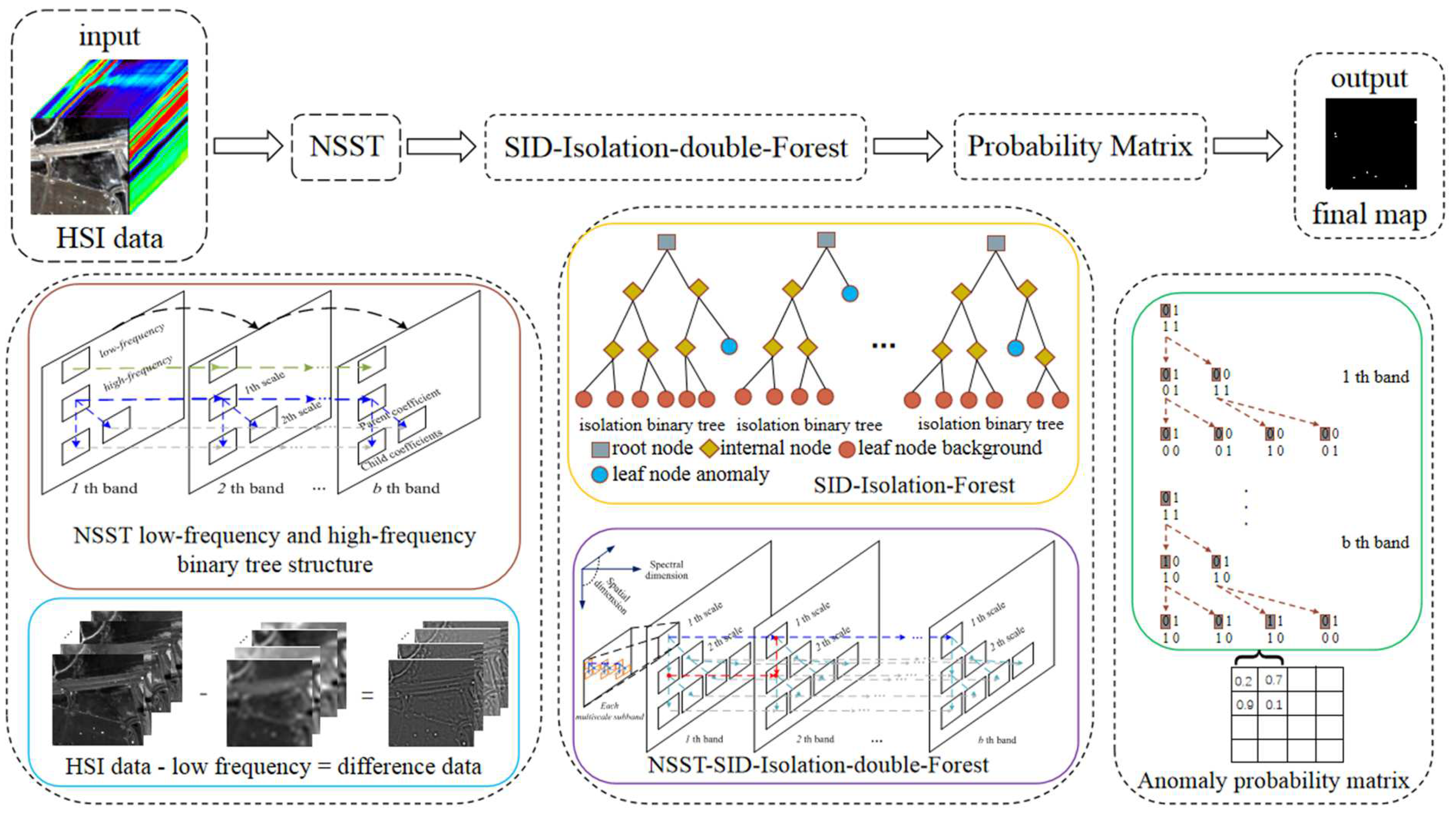
The overall architecture of the proposed SI2FM model in this paper consists of three parts (see Figure 3). (1) NSST is applied to each band of the HIS to obtain the corresponding low-frequency and high-frequency subbands, and then the difference band between the original band and the low-frequency subbands is obtained. Compared with the original band, the difference band can effectively suppress the noise and anomalous interference in the background and enhance the separability of the target and the background. (2) Construct the global and local isolation forest models based on SID attribute for random samples. Improve identification of anomalies by calculating the average value based on the path length several times to obtain the anomaly score. (3) The correlation between the NSST high-frequency subbands of HIS in the spatial and spectral dimensions is mined, and the spatial-spectral 3D forest model structure of these high-frequency subbands is constructed, in which the SID attribute isolation forest anomaly sample coefficient prediction is collaboratively constrained and guided, effectively improving the accuracy of anomaly detection. Section 3.1 to Section 3.2 respectively analyse and illustrate these three components.

3.1. Analysis of Background Suppression in NSST Difference Band

To illustrate the effectiveness of the HIS NSST difference band used in this paper in suppressing background noise and anomalous interference, the ‘maxflat’ NSP multiscale filter and the modified SF are selected to perform 4 directional multiscale decomposition of the 90th band of the Salians dataset [35] to obtain the low- and high-frequency direction subbands, respectively. The transformed subbands are shown in Figure 4, where Figure 4a,b shows the HIS band and the low-frequency subband, respectively, (c) shows the difference band obtained by subtracting the HIS band from the low frequency, (d) shows the anomaly detection reference image, and (e) to (h) show the high-frequency direction subbands in four directions, respectively. From Figure 4, it can be seen that the low frequency contains a lot of background information, while the anomaly information in the difference band is more prominent compared to the HIS band.

Table 1. Parameters of RX methods.

Datasets/AUC	(a)	(b)	(c)
GRX	0.8381	0.5326	0.8978
LRX	0.9475	0.5609	0.9515

shows the area under the curve (AUC) values for comparing the global RX [8] and local RX [10] anomaly detection methods in Figure 4a–c. As can be seen from the table, the difference band has better AUC value than the HSI band, while the low-frequency subband has very low AUC value, indicating that the difference band is better able to suppress background information. Based on this paper, it is argued that the low-frequency subband contains most of the original information of the HSI band and can be regarded as the background image of HSI, and that most of the abnormal target mutation information is contained in the high-frequency subband. Difference band can suppress HSI background information to a certain extent. The background information contained in the high-frequency subband is greatly reduced, and effective detection of the high-frequency subband can well weaken the interference of the background on the anomalous signal during detection and enhance the separability of the target from the background.

In this paper, the NSST decomposition of HSI is carried out in each band. Non-translational invariance of NSST better demonstrates the correspondence between high and low scales, and the intrinsic properties of HSI are explored and modeled according to the characteristics of different subbands and difference bands, providing effective constraints and guidance for improving the separability of anomalous signals and background information and weakening complex backgrounds.

3.2. Isolation Forest Construction Based on SID Attribute

Spectral information divergence (SID) [30] measures the similarity of a spectrum by using the probability difference between two pixels, which is defined as follows.

Assuming that the two given hyperspectral pixel vectors are $\mathrm{x}={\left({\mathrm{x}}_1,\cdots ,{\mathrm{x}}_{\mathrm{B}}\right)}^{\mathrm{T}}$ and $\mathrm{y}={\left({\mathrm{y}}_1,\cdots ,{\mathrm{y}}_{\mathrm{B}}\right)}^{\mathrm{T}}$, respectively, and their corresponding probability vectors are $\mathrm{p}={\left({\mathrm{p}}_1,\cdots ,{\mathrm{p}}_{\mathrm{B}}\right)}^{\mathrm{T}}$ and $\mathrm{q}={\left({\mathrm{q}}_1,\cdots ,{\mathrm{q}}_{\mathrm{B}}\right)}^{\mathrm{T}}$, where $\mathrm{B}$ is the number of bands in the HSI, ${\mathrm{p}}_{\mathrm{i}}=\frac{{\mathrm{x}}_{\mathrm{i}}}{{\sum }_{\mathrm{k}=1}^{\mathrm{B}}{\mathrm{x}}_{\mathrm{k}}}$, ${\mathrm{q}}_{\mathrm{i}}=\frac{{\mathrm{y}}_{\mathrm{i}}}{{\sum }_{\mathrm{k}=1}^{\mathrm{B}}{\mathrm{y}}_{\mathrm{k}}}$, the SID of $\mathrm{x}$ and $\mathrm{y}$ are defined as:

$$\mathrm{SID}\left(\mathrm{x},\mathrm{y}\right)=\mathrm{D}\left(\mathrm{x}\Vert \mathrm{y}\right)+\mathrm{D}\left(\mathrm{y}\Vert \mathrm{x}\right)$$

(1)

where $\mathrm{D}\left(\mathrm{x}\Vert \mathrm{y}\right)$ is the relative entropy of $\mathrm{y}$ with respect to $\mathrm{x}$ and $\mathrm{D}\left(\mathrm{y}\Vert \mathrm{x}\right)$ denotes the relative entropy of $\mathrm{x}$ with respect to $\mathrm{y}$, which is defined as:

$$\left\{\begin{array}{c}\mathrm{D}\left(\mathrm{x}\Vert \mathrm{y}\right)={\displaystyle {\displaystyle \sum }_{\mathrm{i}=1}^{\mathrm{B}}}{\mathrm{p}}_{\mathrm{i}}\log \left(\frac{{\mathrm{p}}_{\mathrm{i}}}{{\mathrm{q}}_{\mathrm{i}}}\right)\\ \mathrm{D}\left(\mathrm{yx}\right)={\displaystyle \sum }_{\mathrm{i}=1}^{\mathrm{B}}{\mathrm{q}}_{\mathrm{i}}\log \left(\frac{{\mathrm{q}}_{\mathrm{i}}}{{\mathrm{p}}_{\mathrm{i}}}\right)\end{array}\right.$$

(2)

SID measures the spectral similarity of the two pixel vectors $\mathrm{x}$ and $\mathrm{y}$ in terms of probability. The larger the value is, the stronger the separability of the two is, and vice versa.

3.2.1. The Global Isolation Forest Construction

Let the size of the HS band group be $\mathrm{M}\times \mathrm{N}\times \mathrm{B}$, where $\mathrm{M}\times \mathrm{N}$ is the size of the band, $\mathrm{B}$ is the number of bands in the band group, and the currently processed band image is ${\mathrm{H}}_{\mathrm{b}}\left(\mathrm{b}\in \left\{1,2,\cdots ,\mathrm{B}\right\}\right)$, whose corresponding low-frequency subband is ${\mathrm{HL}}_{\mathrm{b}}$, high-frequency subband is ${\mathrm{HH}}_{\mathrm{b}}^{\mathrm{l}}$, and difference band is ${\mathrm{HD}}_{\mathrm{b}}$, where$\mathrm{l}\in \left\{1,2,\cdots ,\mathrm{L}\right\},\mathrm{L}$ is the total number of directions of high-frequency subbands in NSST. The process of constructing a global isolation forest based on the SID attribute is as follows:

(1)

Randomly select $\mathsf{\Psi }$ pixels from the HSI as a sample set for constructing a global isolation forest based on SID attribute.

(2)

A binary tree structure is constructed for the pixel points in the sample set based on the size of the SID attribute. That is, the left node ${\mathsf{\Psi }}_{\mathrm{l}}$ and right node ${\mathsf{\Psi }}_{\mathrm{r}}$ are divided: for the current band image ${\mathrm{H}}_{\mathrm{b}}$, its $\mathrm{d}$th pixel point ${\mathrm{H}}_{\mathrm{b}}^{\mathrm{d}}\left(\mathrm{d}\in \left\{1,2,\cdots ,\mathsf{\Psi }\right\}\right)$ is selected, and the SID attribute value $\mathsf{\theta }$ of its subband (which can be ${\mathrm{HL}}_{\mathrm{b}}$ or ${\mathrm{HH}}_{\mathrm{b}}^{\mathrm{l}}$, see Section III.C for details) and the corresponding difference band ${\mathrm{HD}}_{\mathrm{b}}$ is calculated according to Equation (1). When the ${\mathrm{H}}_{\mathrm{b}}^{\mathrm{d}}$ value is less than $\mathsf{\theta }$, the pixel is divided into a left node; otherwise, it is divided into a right node.

(3)

Iterate over the above operations to divide the child nodes, ending the iteration when one of three conditions is met: the height of the tree is limited to ${\log }_2\mathsf{\Psi }$, or there is only one pixel in each child node, or the pixel values in each child node are the same.

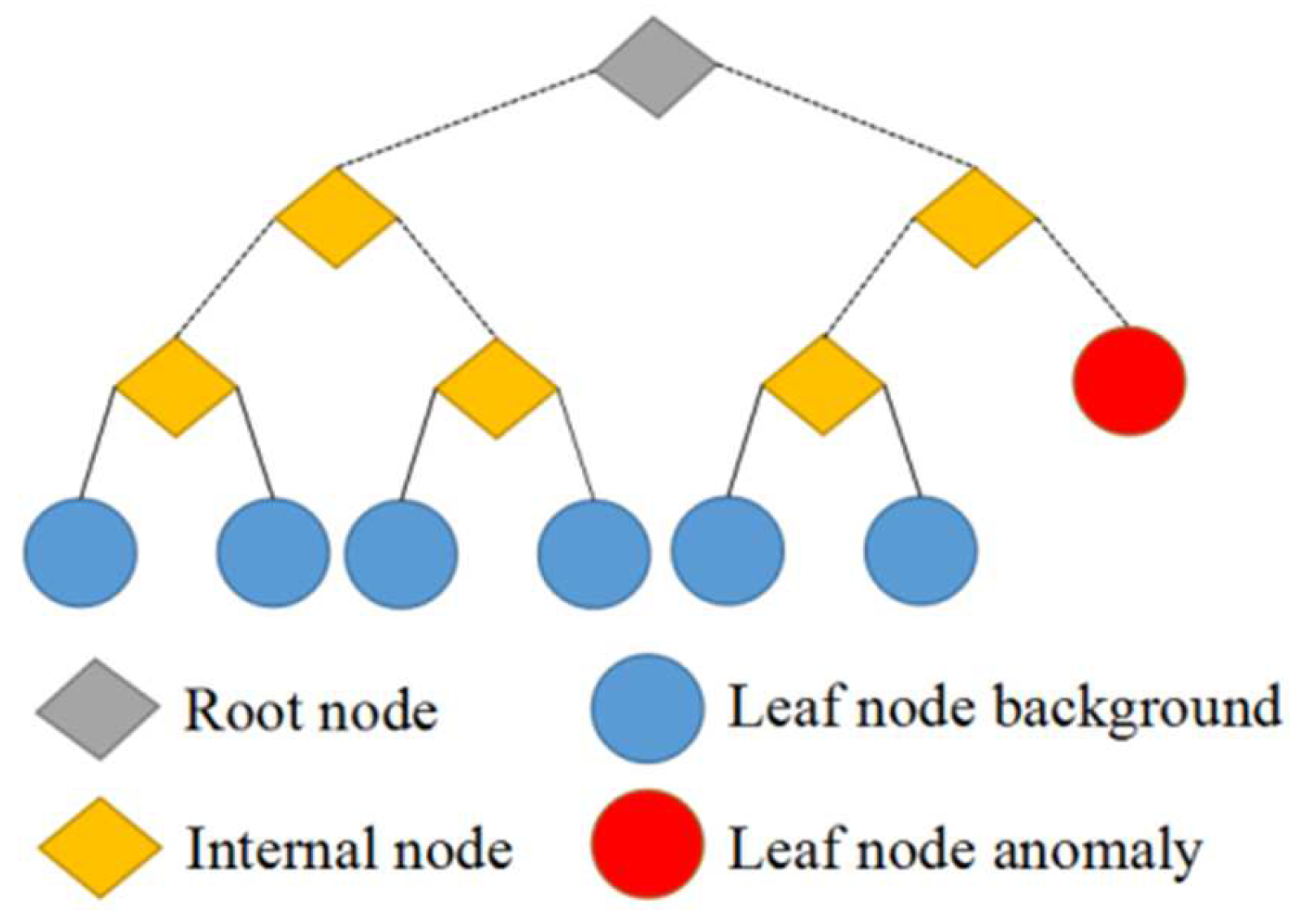
After one round of iterations, an isolation binary tree as shown in Figure 5 will be constructed. Let an isolation forest of $\mathrm{t}$ binary trees be generated after continuous iteration. For each isolation binary tree, the leaf nodes of the background pixels make up the majority of the nodes, and only a small portion are abnormal nodes. The path length of the anomaly pixels is much smaller than the path length of the background pixels.

For a dataset containing $\mathsf{\Psi }$ sample points, the average path length of the constructed isolated binary tree [30] can be calculated by formula (3):

$$\mathrm{c}\left(\mathsf{\Psi }\right)=2\mathrm{H}\left(\mathsf{\Psi }-1\right)-\frac{2\left(\mathsf{\Psi }-1\right)}{\mathsf{\Psi }}$$

(3)

where $\mathrm{H}\left(·\right)$ is the harmonic number estimated by $\ln \left(·\right)+0.5772156649$ (Euler’s constant).

As $\mathrm{c}\left(\mathsf{\Psi }\right)$ is the average of $\mathrm{h}\left(\mathrm{x}\right)$ given $\mathsf{\Psi }$, we use it to normalise $\mathrm{h}\left(\mathrm{x}\right)$. For an instance $\mathrm{x}$, which defines the anomaly score $\mathrm{s}$ for $\mathrm{x}$as:

$$\mathrm{s}\left(\mathrm{x},\mathsf{\Psi }\right)=2^{-\frac{\mathrm{E}\left(\mathrm{h}\left(\mathrm{x}\right)\right)}{\mathrm{c}\left(\mathsf{\Psi }\right)}}$$

(4)

where $\mathrm{E}\left(\mathrm{h}\left(\mathrm{x}\right)\right)$ is the average of $\mathrm{h}\left(\mathrm{x}\right)$ for a collection of isolation trees.

Thus, for the HSI ${\mathrm{H}}_{\mathrm{b}}$, the global isolation forest can be used to obtain anomaly scores, and each anomaly score $\mathrm{s}$can be used as an element to obtain the “initial anomaly detection map” matrix ${\mathrm{D}}_{\mathrm{b}}$.

3.2.2. The Local Isolation Forest Construction

The global isolation forest is constructed from randomly selected data samples from the whole HSI, and the initial anomaly detection results obtained from it may have a high false detection rate. For this reason, this section uses local information from hyperspectral band images and difference bands to construct a local isolation forest [34] to further refine the initial anomaly detection map and obtain further anomaly detection results. The specific procedure is as follows:

(1)

The initial anomaly detection map ${\mathrm{D}}_{\mathrm{b}}\left(\mathrm{b}\in \left\{1,2,\cdots ,\mathrm{B}\right\}\right)$ is binarised and converted to a binary anomaly detection map to obtain ${\mathrm{E}}_{\mathrm{b}}$.

$${\mathrm{E}}_{\mathrm{b}}\left(\mathrm{i},\mathrm{j}\right)=\left\{\begin{array}{c}1, \mathrm{if}{ \mathrm{D}}_{\mathrm{b}}\left(\mathrm{i},\mathrm{j}\right)>\sigma \\ 0, \mathrm{otherwise}\end{array}\right.$$

(5)

where the binarisation threshold $\mathsf{\sigma }$ is determined by the Otsu method [36] and $\left(\mathrm{i},\mathrm{j}\right) \left(\mathrm{i}\in \left\{1,2,\cdots ,\mathrm{M}\right\},\mathrm{j}\in \left\{1,2,\cdots ,\mathrm{N}\right\}\right)$ is the position coordinate.

(2)

According to the binary anomaly detection map ${\mathrm{E}}_{\mathrm{b}}$, the connected domain component of its anomaly can be obtained. Since the area occupied by the anomaly points is scattered and relatively small, for a given area, threshold is $\mathsf{\alpha }$ (in this paper, $\mathsf{\alpha }$ is chosen as $\left(\mathrm{M}\times \mathrm{N}\right)/120$). If the area of the connected region is larger than $\mathsf{\alpha }$, $1/2$ of the pixels in the region are randomly selected as the sample set to construct a local isolation forest and re-evaluate the anomaly scores of the pixel points in the connected region to achieve an update of the initial anomaly detection map ${\mathrm{D}}_{\mathrm{b}}$.

(3)

Iterate the above (1)(2) process until the binary anomaly detection map ${\mathrm{E}}_{\mathrm{b}}$ no longer has any connected areas larger than $\mathsf{\alpha }$, at which point the adjusted ${\mathrm{D}}_{\mathrm{b}}$forms the “refined anomaly detection map” matrix, denoted as ${\mathrm{F}}_{\mathrm{b}}$.

3.2.3. SI2FM

We performed a statistical analysis of the correlation properties of the high-frequency subbands of HSI decomposed by NSST in both spatial and spectral dimensions [32]. By constructing the NSST hidden Markov forest (NSST-HMF) model to characterize the correlation of the coefficients of high-frequency subbands, the correlation of both spatial and spectral dimensional states is considered for the first time on the prediction structure of HSI hidden Markov to synergistically guide the coefficient prediction. A schematics of the NSST high-frequency subband space-spectral dimensional forest construction is given in Figure 6. The following conclusions were obtained as a result.

(1)

The spatial distribution of the NSST high-frequency directional subband coefficients in HSI is persistent and aggregated, as shown by the similarity of the states maintained by the parent coefficients at different scales and in the same directional subbands.

(2)

The distribution of NSST high-frequency directional subband coefficients in the spectral dimension also has a strong continuity and aggregation, so that the NSST directional subband coefficients in the current band of HSI can be used to predict the corresponding directional subband coefficients in the next band (or even the next few bands), but the correlation between the corresponding directional subbands becomes weaker and weaker as the number of decomposition levels increases.

From the above conclusions, it can be seen that the joint spatial-spectral dimensional correlation distribution of subbands in the NSST direction of HIS has a strong aggregation and persistence. The current high-frequency directional subbands are strongly convergent and predictive both for the child subbands in the spatial dimension and for the corresponding co-directional subbands in the spectral dimension. The refined anomaly detection map ${\mathrm{F}}_{\mathrm{b}}$ obtained from Section 3.2.2. If the parent coefficients are anomalous, the child coefficients will also be anomalous with a high probability. Similarly, if a point in the current band is anomalous, there is a high probability that the same location in the subsequent band will also be anomalous.

Accordingly, for the low-frequency subband ${\mathrm{HL}}_{\mathrm{b}}$ and high-frequency subband ${\mathrm{HH}}_{\mathrm{b}}^{\mathrm{l}}$ corresponding to the band ${\mathrm{H}}_{\mathrm{b}}$, the corresponding refined anomaly detection map matrices ${\mathrm{F}}_{\mathrm{b}\_\mathrm{HL}}$ and ${\mathrm{F}}_{\mathrm{b}\_\mathrm{HH}}^{\mathrm{l}}$ were obtained by the joint differential band for ${\mathrm{HD}}_{\mathrm{b}}$ through the global and local isolation forest construction process based on SID attribute in Section 3.2.1 and Section 3.2.2, respectively. Further, the probability of the same position value of 1 for ${\mathrm{F}}_{\mathrm{b}\_\mathrm{HL}}$ and ${\mathrm{F}}_{\mathrm{b}\_\mathrm{HH}}^{\mathrm{l}}$ is statistically calculated to construct the probability matrix ${\mathrm{F}}_{\mathrm{map}}$, and the final anomaly detection result matrix ${\mathrm{F}}_{\mathrm{final}\_\mathrm{map}}$ is determined by selecting the threshold value $\mathsf{\delta }$ based on the Otsu method:

$${\mathrm{F}}_{\mathrm{final}\_\mathrm{map}}\left(\mathrm{his},\mathrm{j}\right)=\left\{\begin{array}{c}1,{ \mathrm{if} \mathrm{F}}_{\mathrm{map}}\left(\mathrm{his},\mathrm{j}\right)>\mathsf{\delta }\\ 0, \mathrm{o}\mathrm{t}\mathrm{h}\mathrm{e}\mathrm{r}\mathrm{w}\mathrm{i}\mathrm{s}\mathrm{e} \end{array}\right.$$

(6)

where $\left(\mathrm{his},\mathrm{j}\right) \left(\mathrm{i}\in \left\{1,2,\cdots ,\mathrm{M}\right\},\mathrm{j}\in \left\{1,2,\cdots ,\mathrm{N}\right\}\right)$ is the position coordinate.

Isolation forest is used for data anomaly detection mining, where the values of attributes that are different from the background are isolated from the perspective of anomalies, so that the anomalies can be separated more easily than the background. In order to make the detection accuracy more accurate, we combine NSST with isolation forest. The correlation between the space-spectral dimension coefficients of high-frequency subbands uses NSTT. In the spatial dimension, if its parent coefficient is anomalous, its child coefficient will also be anomalous with high probability, and in the spectral dimension, if a position in the current band is anomalous, the same position in the subsequent band will also be anomalous with high probability. The construction and detection of isolation forests in 3D space suppress the background information in HS and improve the detection accuracy of the method.

Based on the above analysis, this paper proposes the SI2FM HIS-AD method based on the isolation forest model with SID attribute and the NSST high-frequency subband spatial-spectral 3D forest model, and the method description is given in Algorithm 1.

Algorithm 1: SI2FM$\left(H,L,t,\psi \right)$

Input:${\mathrm{H}}_{\mathrm{b}}\left(\mathrm{b}\in \left\{1,2,\cdots ,\mathrm{B}\right\}\right)$- input HIS H with the size of $M\times N\times B$, $L$—NSST decomposition layers, $t$—number of trees, $\psi$—sub-sampling size.

for all bands do

1: For each band, $H_b$ is decomposed by $L$-scale NSST to obtain low-frequency $H{L}_b$and high-frequency $H{H}_b^l$ $\left(l\in \left\{1,2,\cdots ,L\right\}\right)$ binary tree structure and difference data $H{D}_b$;

2: Calculation the value of SID of each ${\mathrm{HD}}_{\mathrm{b}}$ and low-frequency ${\mathrm{HL}}_{\mathrm{b}}$, high-frequency ${\mathrm{HH}}_{\mathrm{b}}^{\mathrm{l}}$ by Equation (1);

3: Construct the SID global isolated forest by ${\mathrm{HL}}_{\mathrm{b}}$and ${\mathrm{HH}}_{\mathrm{b}}^{\mathrm{l}}$;

4: Calculate the $D_{b\_HL}$ of each ${\mathrm{HL}}_{\mathrm{b}}$ and ${\mathrm{HD}}_{\mathrm{b}}$ by SID-Global-iForest Equation (4);

5: Calculate the $D_{b\_HH}^l$ of each ${\mathrm{HH}}_{\mathrm{b}}^{\mathrm{l}}$ and ${\mathrm{HD}}_{\mathrm{b}}$ by SID-Global-iForest Equation (4);

6: Calculate the $F_{b\_HL}$ of each ${\mathrm{HL}}_{\mathrm{b}}$ and ${\mathrm{HD}}_{\mathrm{b}}$ by Local-iForest Equation (5);

7: Calculate the $F_{b\_HH}^l$ of each ${\mathrm{HH}}_{\mathrm{b}}^{\mathrm{l}}$ and ${\mathrm{HD}}_{\mathrm{b}}$by Local-iForest Equation (5);

end for

8: Calculate the final anomaly detection result $F_{final\_map}$by Equation (6);

Output: anomaly detection map $F_{\mathrm{final}\_\mathrm{map}}$.

4. Experiment and Analysis

The experimental environment is Windows 7, the computer is equipped with a 3.3 GHz Core i5-4590 processor and 8G RAM, the experimental platform is Matlab 2014b. Experimental image data cropping was processed using ENVI 5.1 software.

4.1. Dataset

In this paper, four real HIS captured from different scenes [9] are selected to evaluate the proposed method, and Figure 7 shows the pseudo-color image and the corresponding reference detection map, respectively. The experimental datasets are all remote sensing data images with noise bands removed.

(1)

HYDICE Urban: The data were acquired from the hyperspectral digital imagery collection experiment (HYDICE) sensor and were taken in an urban area in California, USA. The experimental data have a scene size of $80\times 80$, with 175 bands where the noise bands have been removed, and spatial resolution of 2 m and spectral resolution of 10 nm. They also contains 20 anomalous pixels for cars and roofs.

(2)

Texas Coast: Acquired from the AVIRIS sensor, captured in the Texas coastal metropolitan area; flight time was 29 August 2010. The experimental dataset in this paper is $100\times 100\times 204$ in size and 17.2 m in spatial resolution; this dataset contains 67 anomalous pixels from the aircraft scene.

(3)

Gulfport Airport: The dataset from the AVIRIS sensor capturing the Gulfport airport area; flight time was 7 July 2010. The scene size of the experimental dataset in this paper is $100\times 100$, 191 spectral channels with a spatial resolution of 3.4m; this dataset contains 60 anomalous pixels from the aircraft scene.

(4)

Cat Island: It is obtained from the AVIRIS sensor, and the beach and sea area of Cat Island is photographed. Flight time was 12 September 2010. The size of the experimental dataset is $150\times 150\times 188$ and the spatial resolution is 17.2 m. The data contain 19 abnormal pixels from the aircraft scene.

4.2. Parameter Analysis

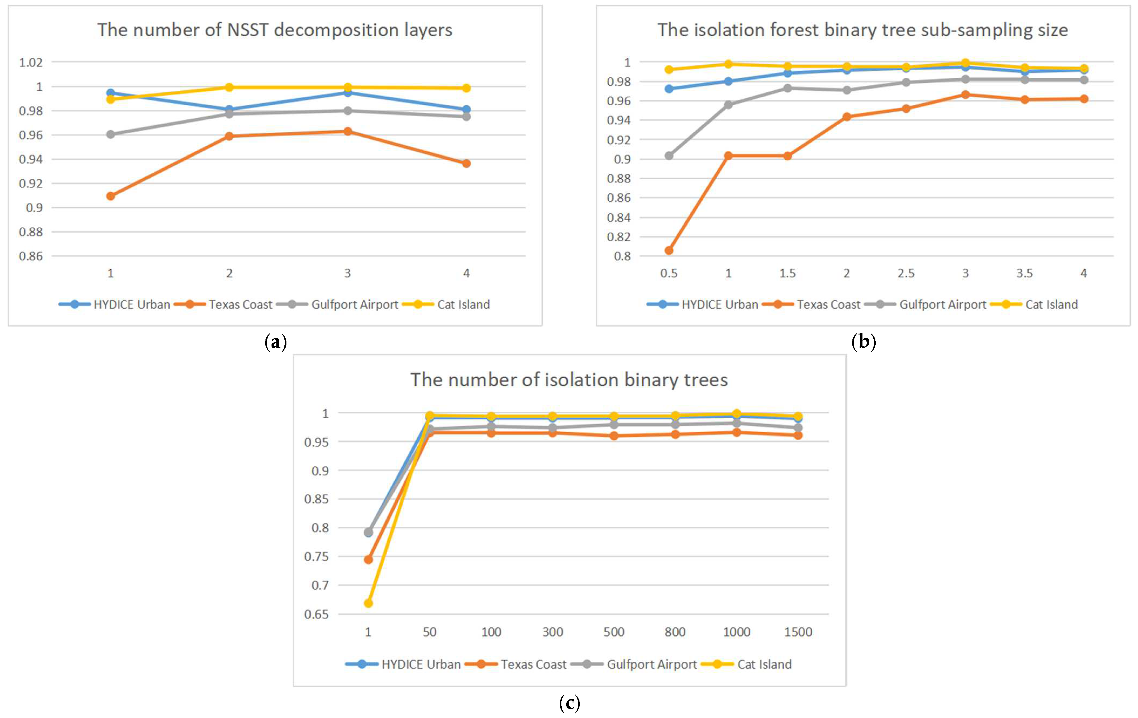
The proposed SI2FM algorithm involves three important parameters, including the number of NSST decomposition layers $L$, building an isolation forest binary tree sub-sampling size $\mathsf{\Psi }$, and the number of isolation binary trees $t$. Based on the AUC, we evaluate the impact of different parameter settings on SI2FM using the HYDICE Urban, Texas Coast, Gulfport Airport, and Cat Island datasets as examples; the AUC line graph of the SI2FM algorithm with parameter variation is given in Figure 8.

(1)

The number of NSST decomposition layers $L$: Figure 8a gives a line graph of the variation of the AUC value of the SI2FM algorithm with parameter $L$. From the graph, it can be seen that the optimal AUC is obtained when $L=3$. For the property that the correlation between coefficients becomes smaller as the number of layers of NSST decomposition increases, the value of AUC may become smaller and smaller when $L$ is greater than 4. The results obtained from the Texas Coast dataset are particularly obvious, so in this experiment, $L=3$ was chosen as the optimal parameter based on the experimental data, and binary trees were constructed with scale directions of 2, 4, and 8 for each layer.

(2)

The isolation forest binary tree sub-sampling size $\Psi$: Figure 8b shows a line graph of the variation of the AUC value of the SI2FM algorithm with the parameter $\mathsf{\Psi }$ (percentage of total pixels in the image). It can be seen from the figure that for the HYDICE Urban and Gulfport Airport, the overall trend of the AUC values is to increase first and then decrease, with their AUC being at the optimum when $\mathsf{\Psi }=3$. The Texas Coast has an overall increasing trend in AUC when $\mathsf{\Psi }$is less than 3, and plateaus when $\mathsf{\Psi }$ is greater than 3. For Cat Island, the overall area is flat and the AUC reaches a peak at $\mathsf{\Psi }=3$. Therefore, $\mathsf{\Psi }=3$ was chosen as the default parameter value for the experiments in this paper.

(3)

The number of isolation binary trees t: Figure 8c shows the line graph of the AUC value of the SI2FM algorithm as the parameter t changes. From the graph, it can be seen that when t changes from 1 to 500, the overall trend shows an upward trend, and when t continues to increase to 1000, the overall trend tends to a stable state, so this implementation chooses t = 1000 as the default parameter value.4.3. Comparison and Analysis of Detection Performance

4.3. Comparison and Analysis of Detection Performance

This section selects 11 state-of-the-art anomaly detection algorithms for comparative experiments, including: RX algorithm [8], LRX algorithm [10], the unsupervised nearest regularized subspace (UNRS) algorithm [13], CRD algorithm [14], LSAD algorithm [17], the local summation unsupervised nearest regularized subspace with an outlier removal anomaly detector (LSUNRSORAD) algorithm [37], the local summation anomaly detection based on collaborative representation and inverse distance weight (LSAD -CR-IDW) algorithm [37], the CRD with background purification and saliency weight (CRDBPSW) algorithm [16], the feature extraction and background purification for anomaly detection (FEBPAD) algorithm [18], the visual attention and background subtraction (VABS) algorithm [19], and the kernel isolation forest-based hyperspectral anomaly detection (KIFD) algorithm [34].

In order to effectively evaluate the proposed method, we referred to the comparison literature and conducted experiments on four real hyperspectral datasets. We tried to keep all parameters the same in different methods to make the comparison parameters as optimal as possible; the comparison algorithm parameter settings and related papers are provided as shown in

Table 2. Parameters of different detection methods.

Method	Parameters
RX	—
LRX	$wi{n}_{out}=5,wi{n}_{in}=3$
UNRS	$\lambda =0.01,wi{n}_{out}=5,wi{n}_{in}=3$
CRD	$\lambda =0.01,wi{n}_{out}=5,wi{n}_{in}=3$
LSAD	$wi{n}_{out}=5$
LSUNRSORAD	$\lambda =0.01,wi{n}_{out}=5,wi{n}_{in}=3$
LSAD-CR-IDW	$\lambda =0.01,wi{n}_{out}=5,wi{n}_{in}=3$
CRDBPSW	$\lambda =0.01,wi{n}_{out}=5,wi{n}_{in}=3$
FEBPAD	$p=0.7,r=3,k=0.7\times m\times n$
VABS	$L=5,T=1000,c\mathsf{\epsilon }\left\{1,2,3\right\},\mathsf{\epsilon }\mathsf{\epsilon }\left\{1,2\right\}$
KIFD	$M=0.03\times N,q=1000,\mathsf{\zeta }=300$

.

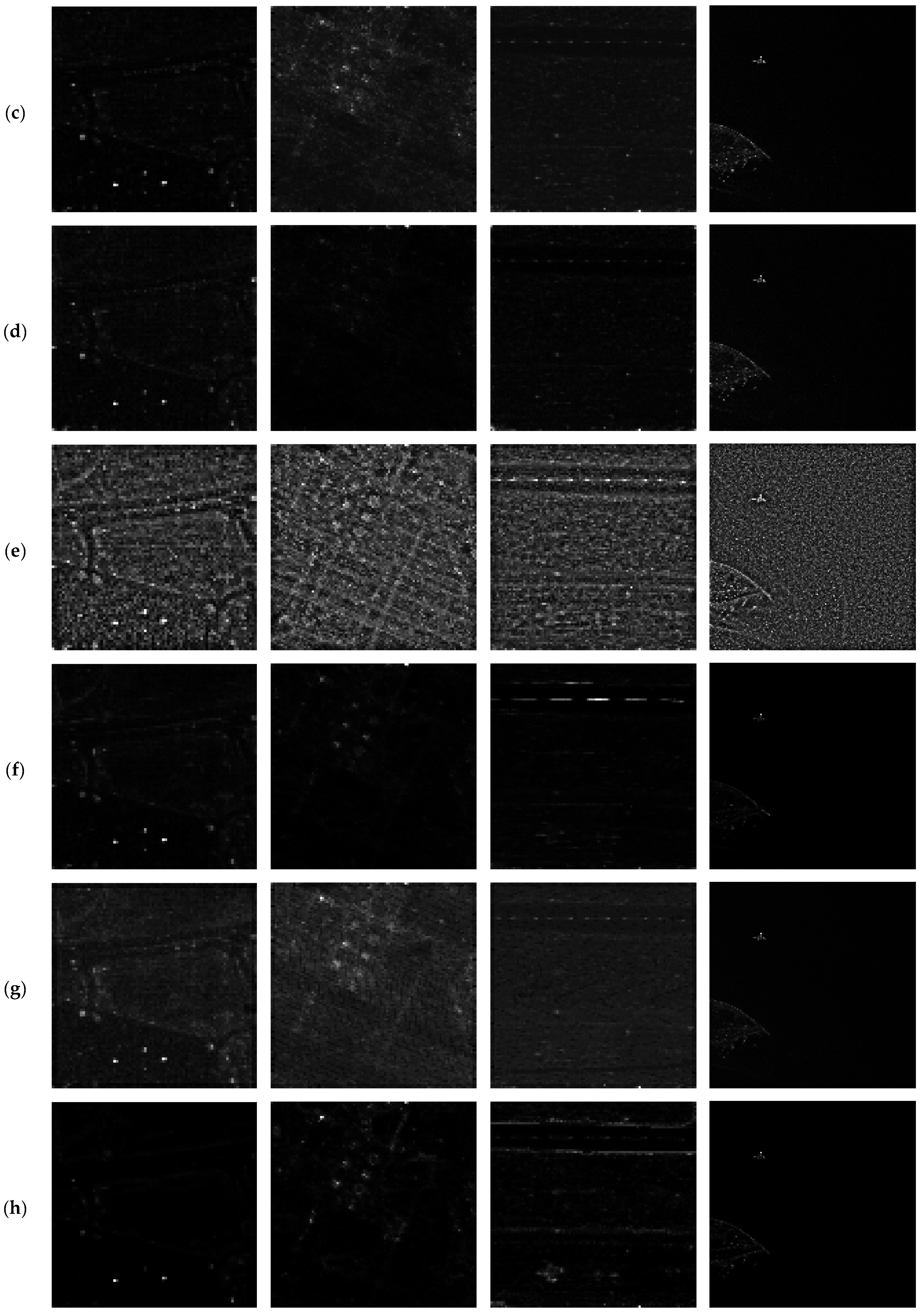
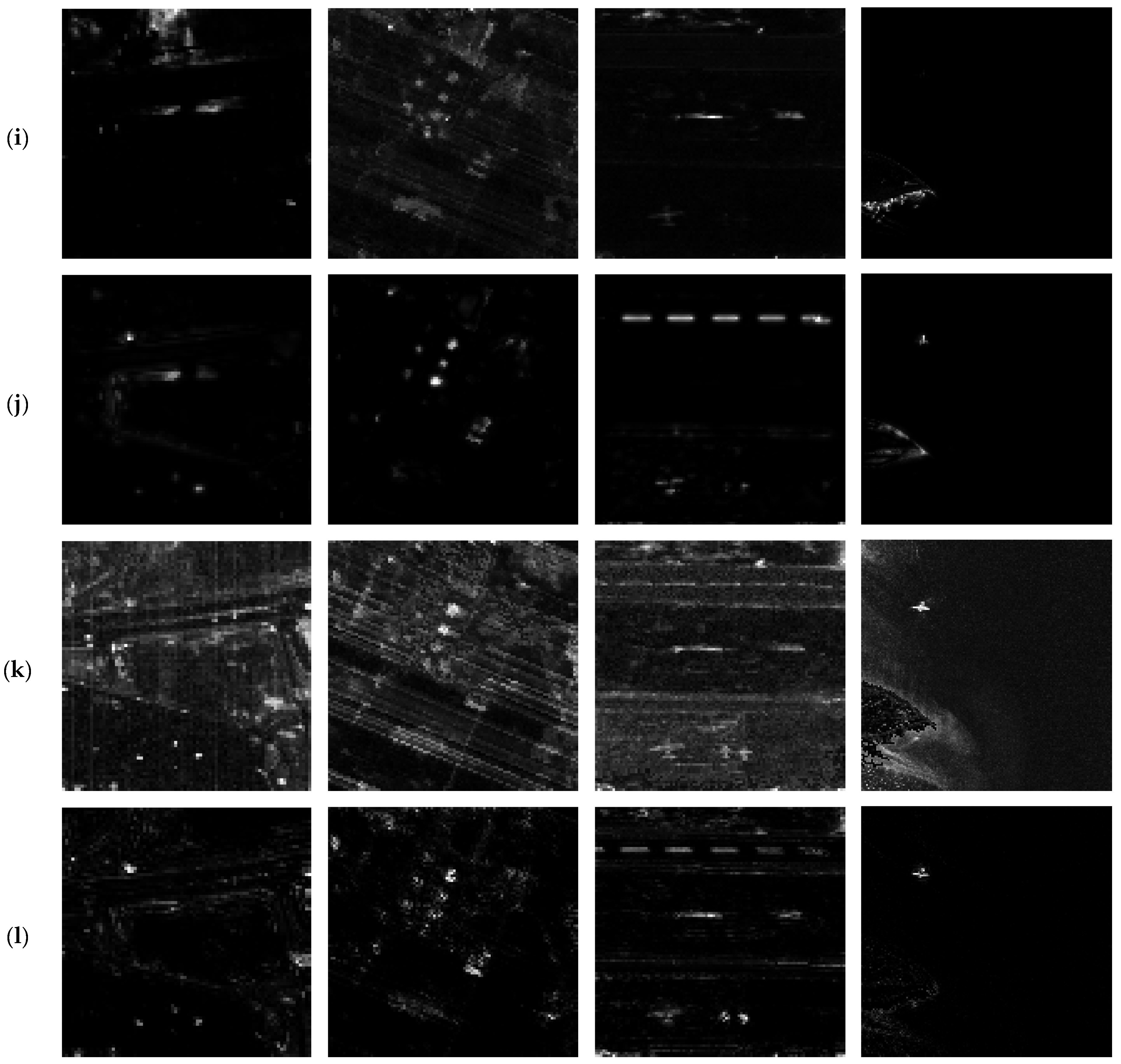
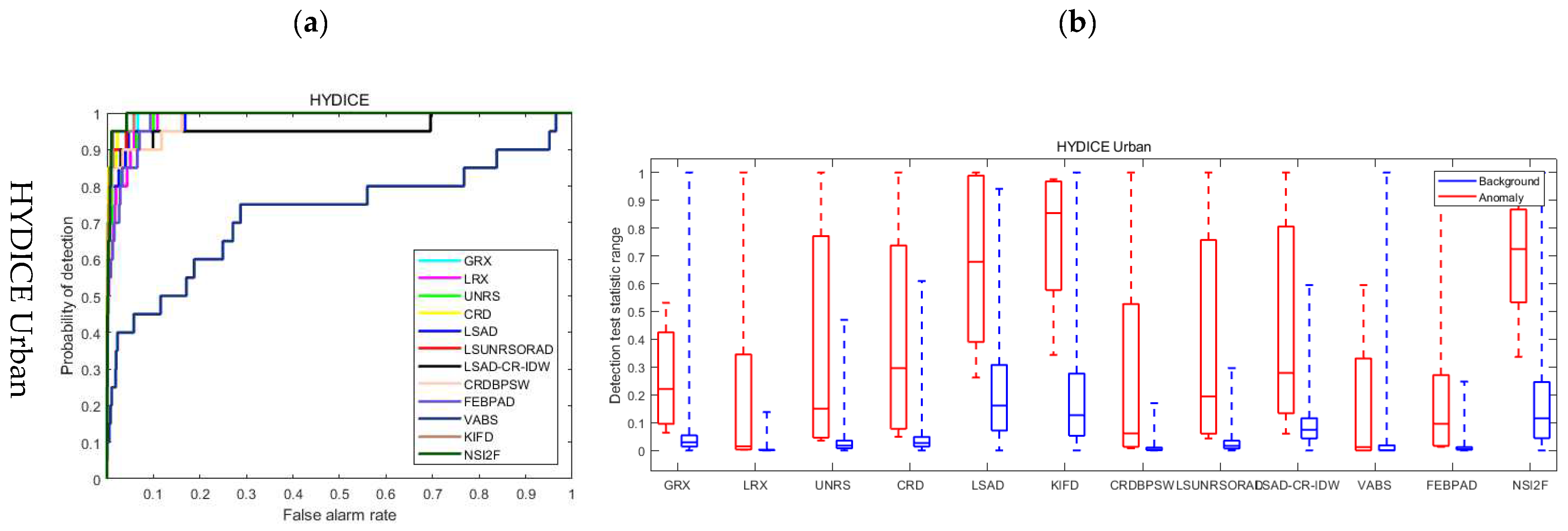
The results of the subjective comparative evaluation of HIS-AD for the four experimental datasets are shown in Figure 9, and the corresponding ROC curves [38] and target background separation boxplot [37] are given in Figure 10.

Table 3. AUC of each algorithm for four datasets.

Datasets	AUC
	HYDICE Urban	Texas Coast	Gulfport Airport	Cat Island
RX	0.9908	0.9906	0.9526	0.9807
LRX	0.9832	0.8736	0.8235	0.9956
UNRS	0.9863	0.9722	0.7916	0.9936
CRD	0.9925	0.9655	0.7681	0.9928
LSAD	0.9853	0.9201	0.8464	0.9414
LSUNRSORAD	0.9926	0.9962	0.9589	0.9935
LSAD-CR-IDW	0.9564	0.9824	0.8335	0.9943
CRDBPSW	0.9817	0.9741	0.9531	0.9941
FEBPAD	0.9815	0.9432	0.9494	0.9428
VABS	0.7384	0.9161	0.9325	0.9962
KIFD	0.9945	0.9325	0.9759	0.9899
SI2FM	0.9947	0.9664	0.9823	0.9992

shows the objective evaluation for the different methods of AUC values.

In the case of the HYDICE Urban, as shown in the ROC curve in Figure 10a, SI2FM has a better ability to identify anomalous targets compared to other methods. Table III also shows the best AUC values. The separability between the anomaly and the background is shown in Figure 10b. Both the proposed method and KIFD can effectively separate the background from the anomalous features and make the anomalies clearer on the detection map, but SI2FM is more effective in background suppression and has a better ability to identify anomalous targets compared to KIFD. From Figure 7, the anomaly detection results of the SI2FM algorithm are also the closest to the reference image, providing better detection performance compared to other methods.

For the Texas Coast, as shown in the ROC curves in Figure 10a, the algorithms of RX, UNRS, LSUNRSORAD, LSAD-CR -IDW, CRDBPSW, and SI2FM are all relatively good at identifying anomalous targets. The target background separation boxplot in Figure 10b shows that GRX is optimal, but that LSUNRSORAD and SI2FM are more effective in terms of background suppression, with a more complex background for the Texas Coast. It is clear from Figure 7 that the SI2FM can detect more anomaly pixels than the LSUNRSORAD.

For the Gulfport Airport, as shown in the ROC curve in Figure 10a, SI2FM has a better ability to identify anomaly compared to other methods, as is well-evidenced by the objective evaluation of Table 3. Figure 10b shows that KIFD and SI2FM are more effective in terms of anomaly and background separability, but SI2FM is more prominent in terms of background suppression. In Figure 9, we can see that SI2FM and KIFD are able to identify anomalous targets, but KIFD has relatively more noise.

In the case of the Cat Island dataset, the best AUC values were obtained in the objective evaluation for Table 3. As shown in the ROC curve in Figure 10a, SI2FM has a better ability to identify anomalous targets compared to other methods. Figure 10b shows that both the proposed method and KIFD are effective in separating background and anomalous features, making the anomalies clearer on the detection map, but SI2FM is more effective in background suppression and has a better ability to identify anomaly than KIFD. From Figure 9, the anomaly detection results of the SI2FM algorithm are also the closest to the reference image, providing better detection performance compared to other methods.

4.4. Ablation Study

In this section, a detailed ablation study of the SI2FM framework is performed to further investigate the validity of the proposed model.

SI2FM framework consists of the SID global isolation forest model, the local isolation forest model, and the NSST 3D spatial-spectral dimensional forest model.

To test the effects of the three components on the anomaly detection effectiveness, we conducted an ablation experiment to evaluate the performance of the proposed model. As shown in

Table 4. Ablation study of the proposed models.

Framework	AUC
	HYDICE Urban	Texas Coast	Gulfport Airport	Cat Island
the SID global isolation	0.9440	0.9635	0.9565	0.9920
the SID local isolation	0.9459	0.9779	0.9798	0.9925
SI2FM	0.9447	0.9664	0.9823	0.9992

, the AUC evaluation performance values are calculated separately for the SID global isolation model, the SID local isolation model, and the SI2FM model. It can be seen that both the SID local isolation model and the NSST forest model contribute to the performance of the isolation forest model.

Compared with the original global isolation forest model, both compositional frameworks help to improve the model performance and validity for hyperspectral experimental data.

5. Conclusions

In this paper, we propose an HSI-AD method based on SI2FM. Firstly, the difference band formed between the original HSI band and its NSST low-frequency subband is used as a guide, the global isolation forest and local isolation forest models are constructed based on the SID attribute values of the difference band and the low-frequency high-frequency subbands, and the anomaly scores are determined by evaluating the path lengths of the isolation binary tree nodes in the forest model to obtain a progressively optimized anomaly detection map. Secondly, based on the persistence and aggregation of the high-frequency subband coefficients of HSI decomposed by NSST in both spatial-spectral dimensions, the NSST high-frequency subband spatial-spectral dimensional forest structure relationship is used to achieve the co-optimization of multiple anomaly detection maps obtained from the isolation forest, which effectively improves the accuracy of anomaly detection. The effectiveness of the algorithm is verified by comparing real hyperspectral datasets captured in four different scenes with eleven typical anomaly detection algorithms currently available.

It should be noted that the SI2FM algorithm is suitable for small target scenes, but for noise-laden hyperspectral datasets, the algorithm in this paper has no noise reduction effect; according to the isolation forest it is easy to identify isolated anomalies. It will be easy to show the noisy points as anomalies; the above experiments are conducted on the dataset without noise bands. For conditions where noise appears in the image due to atmospheric conditions, the ability to check the noise based on its power and spectral composition will also be an area for further optimization. In any case, the computational costs of the proposed algorithm are still significant and this is the focus of future work.

References

1. Ghamisi, P.; Yokoya, N.; Li, J.; Liao, W.; Liu, S.; Plaza, J.; Rasti, B.; Plaza, A. Advances in hyperspectral image and signal processing: A comprehensive overview of the state of the Art. IEEE Geosci. Remote Sens. Mag. 2018, 5, 37–78. [Google Scholar] [CrossRef] [Green Version]
2. Kriti, G.U. A comprehensive review of HSI in diverse research domains. Mater. Today Proc. 2021. [Google Scholar] [CrossRef]
3. Chang, C.I. Hyperspectral target detection: Hypothesis testing, signal-to-noise ratio, and spectral angle theories. IEEE Trans. Geosci. Remote Sens. 2022, 60, 1–23. [Google Scholar] [CrossRef]
4. Chang, C.I.; Wang, Y.L.; Xue, B. Hyperspectral Target Detection: Algorithm Design and Analysis; Hubei Science & Technology Press: Wuhan, China, 2021. [Google Scholar]
5. Racetin, I.; Krtali, A. Systematic review of anomaly detection in hyperspectral remote sensing applications. Appl. Sci. 2021, 11, 4878. [Google Scholar] [CrossRef]
6. Su, H.; Wu, Z.; Zhang, H.; Du, Q. Hyperspectral anomaly detection: A survey. IEEE Geosci. Remote Sens. Mag. 2022, 10, 64–90. [Google Scholar] [CrossRef]
7. Chang, C.I. Hyperspectral anomaly detection: A dual theory of hyperspectral target detection. IEEE Trans. Geosci. Remote Sens. 2022, 60, 1–20. [Google Scholar] [CrossRef]
8. Reed, I.S.; Yu, X. Adaptive multiple-band CFAR detection of an optical pattern with unknown spectral distribution. IEEE Trans. Acoust. Speech Signal Process. 1990, 38, 1760–1770. [Google Scholar] [CrossRef]
9. Borghys, D.; Kåsen, I.; Achard, V.; Perneel, C. Comparative evaluation of hyperspectral anomaly detectors in different types of background. In Proceedings of the Algorithms and Technologies for Multispectral, Hyperspectral, and Ultraspectral Imagery XVIII, Baltimore, MD, USA, 24 May 2012. [Google Scholar]
10. Molero, J.M.; Garzon, E.M.; Garcia, I.; Plaza, A. Analysis and optimizations of global and local versions of the RX algorithm for anomaly detection in hyperspectral data. IEEE J. Sel. Top. Appl. Earth Obs. Remote Sens. 2013, 6, 801–814. [Google Scholar] [CrossRef]
11. Riley, R.A.; Newsom, R.K.; Andrews, A.K. Anomaly Detection in Noisy Hyperspectral Imagery; SPIE: Bellingham, WA, USA, 2004; Volume 5546, pp. 159–170. [Google Scholar] [CrossRef]
12. Kwon, H.; Nasrabadi, N.M. Kernel RX-algorithm: A nonlinear anomaly detector for hyperspectral imagery. IEEE Trans. Geosci. Remote Sens. 2005, 43, 388–397. [Google Scholar] [CrossRef]
13. Li, W.; Du, Q. Unsupervised nearest regularized subspace for anomaly detection in hyperspectral imagery. In Proceedings of the IEEE International Geoscience and Remote Sensing Symposium—IGARSS, Melbourne, VIC, Australia, 21–26 July 2013. [Google Scholar] [CrossRef]
14. Li, W.; Du, Q. Collaborative representation for hyperspectral anomaly detection. IEEE Trans. Geosci. Remote Sens. 2015, 53, 1463–1474. [Google Scholar] [CrossRef]
15. Hou, Z.; Li, W.; Tao, R. Collaborative representation with background purification and saliency weight for hyperspectral anomaly detection. Sci. China Inf. Sci. 2022, 65, 112305. [Google Scholar] [CrossRef]
16. Hou, Z.; Li, W.; Gao, L.; Zhang, B.; Ma, P.; Sun, J. A background refinement collaborative representation method with saliency weight for hyperspectral anomaly detection. In Proceedings of the IEEE International Geoscience and Remote Sensing Symposium, Waikoloa, HI, USA, 26 September–2 October 2020. [Google Scholar] [CrossRef]
17. Du, B.; Zhao, R.; Zhang, L. A spectral-spatial based local summation anomaly detection method for hyperspectral images. Signal Process. 2016, 124, 115–131. [Google Scholar] [CrossRef]
18. Ma, Y.; Fan, G.; Jin, Q.; Huang, J.; Mei, X.; Ma, J. Hyperspectral anomaly detection via integration of feature extraction and background purification. IEEE Geosci. Remote Sens. Lett. 2021, 18, 1436–1440. [Google Scholar] [CrossRef]
19. Xiang, P.; Song, J.; Qin, H.; Tan, W.; Li, H.; Zhou, H. Visual attention and background subtraction with adaptive weight for hyperspectral anomaly detection. IEEE J. Sel. Top. Appl. Earth Obs. Remote Sens. 2021, 14, 2270–2283. [Google Scholar] [CrossRef]
20. Feng, S.; Tang, S.; Zhao, C. A Hyperspectral Anomaly Detection Method Based on Low-Rank and Sparse Decomposition with Density Peak Guided Collaborative Representation. IEEE Trans. Geosci. Remote Sens. 2022, 60, 1–13. [Google Scholar] [CrossRef]
21. Wang, M.; Wang, Q.; Hong, D.; Roy, S.K.; Chanussot, J. Learning Tensor Low-Rank Representation for Hyperspectral Anomaly Detection. IEEE Trans. Cybern. 2023, 53, 679–691. [Google Scholar] [CrossRef]
22. Song, X. Spectral-Spatial Anomaly Detection of Hyperspectral Data Based on Improved Isolated Forest. IEEE Trans. Geosci. Remote Sens. 2022, 60, 1–16. [Google Scholar]
23. Arisoy, S.; Nasrabadi, N.M.; Kayabol, K. Unsupervised Pixel-Wise Hyperspectral Anomaly Detection via Autoencoding Adversarial Networks. IEEE Geosci. Remote Sens. Lett. 2022, 19, 1–15. [Google Scholar] [CrossRef]
24. Zhang, L.; Cheng, B. Transferred CNN based on tensor for hyperspectral anomaly detection. IEEE Geosci. Remote Sens. Lett. 2020, 17, 2115–2119. [Google Scholar] [CrossRef]
25. Arisoy, S.; Nasrabadi, N.M.; Kayabol, K. GAN-based hyperspectral anomaly detection. In Proceedings of the 2020 28th European Signal Processing Conference (EUSIPCO), Amsterdam, Netherlands, 18–21 January 2021. [Google Scholar] [CrossRef]
26. Guoand, K.; Labate, D. Optimally sparse multidimensional representation using shearlets. SIAMJ. Math. Anal. 2007, 39, 298–318. [Google Scholar]
27. Easley, G.; Labate, D.; Lim, W.-Q. Sparse directional image representations using the discrete shearlet transform. Appl. Comput. Harmon. Anal. 2008, 25, 25–46. [Google Scholar] [CrossRef] [Green Version]
28. Lim, W.Q. Nonseparable shearlet transform. IEEE Trans. Image Process. 2013, 22, 2056–2065. [Google Scholar]
29. Karami, A.; Soleimanzadeh, M.R. Hyperspectral image classification using nonsubsampled shearlet transform. Image Signal Process. Remote Sens. 2017. [Google Scholar] [CrossRef]
30. Soleimanzadeh, M.R.; Karami, A.; Scheunders, P. Fusion of hyperspectral and lidar images using non-subsampled shearlettransform. In Proceedings of the IEEE International Geoscience and Remote Sensing Symposium, Valencia, Spain, 22–27 July 2018. [Google Scholar] [CrossRef]
31. Li, L.; Si, Y. Enhancement of hyperspectral remote sensing images based on improved fuzzy contrast in nonsubsampled shearlet transform domain. Multimed. Tools Appl. 2019, 78, 18077–18094. [Google Scholar] [CrossRef]
32. Wang, X.; Mu, Z.; Song, R.; Tao, J.; Song, C. A hyperspectral image NSST-HMF model and its application in HS-Pansharpening. IEEE Trans. Geosci. Remote Sens. 2020, 58, 4803–4817. [Google Scholar] [CrossRef]
33. Liu, F.T.; Ting, K.M.; Zhou, Z. Isolation forest. In Proceedings of the 8th IEEE International Conference on Data Mining, Pisa, Italy, 15–19 December 2008. [Google Scholar]
34. Li, S.; Zhang, K.; Duan, P.; Kang, X. Hyperspectral anomaly detection with kernel isolation forest. IEEE Trans. Geosci. Remote Sens. 2020, 58, 319–329. [Google Scholar] [CrossRef]
35. Yuan, Y.; Wang, Q.; Zhu, G. Fast hyperspectral anomaly detection via high-order 2-D crossing filter. IEEE Trans. Geosci. Remote Sens. 2014, 53, 620–630. [Google Scholar] [CrossRef]
36. Otsu, N. A shreshold selection method from gray-level histograms. IEEE Trans. Syst. Man Cybern. 1979, 9, 62–66. [Google Scholar] [CrossRef]
37. Tan, K.; Hou, Z.; Wu, F.; Du, Q.; Chen, Y. Anomaly detection for hyperspectral imagery based on the regularized subspace method and collaborative representation. Remote Sens. 2019, 11, 1318. [Google Scholar] [CrossRef] [Green Version]
38. Hanley, J.A.; Mcneil, B.J. The meaning and use of the area under a receiver operating characteristic (ROC) curve. Radiology 1982, 143, 29–36. [Google Scholar] [CrossRef]
Figure 1. The flow chart of the NSST Transform.
Remotesensing 15 00612 g001
Figure 2. Diagram of the splitting point. (a) Anomaly splitting; (b) Normal point splitting.
Remotesensing 15 00612 g002
Figure 3. Flow chart of the proposed SI2FM-HIS-AD framework.
Remotesensing 15 00612 g003
Figure 4. NSST subbands and difference band in the HSI band. (a) HSI band; (b) Low-frequency subband; (c) Difference band; (d) Anomaly detection reference map; (e) High-frequency subband in direction 1; (f) High-frequency subband in direction 2; (g) High-frequency subband in direction 3; (h) High-frequency subband in direction 4.
Remotesensing 15 00612 g004aRemotesensing 15 00612 g004b
Figure 5. Example illustration the structure of an iTree.
Remotesensing 15 00612 g005
Figure 6. Illustration of NSST high-frequency subbands spatial spectral dimensional forest construction.
Remotesensing 15 00612 g006
Figure 7. Experimental dataset.
Remotesensing 15 00612 g007
Figure 8. Influence of different parameters on SI2FM algorithm detection performance. (a) The number of NSST decomposition layers; (b) The isolation forest binary tree sub-sampling size; (c) The number of isolation binary trees.
Remotesensing 15 00612 g008
Figure 9. I-AD maps on four datasets. (a) RX; (b) LRX; (c) UNRS; (d) CRD; (e) LSAD; (f) LSUNRSORAD; (g) LSAD-CR-IDW; (h) CRDBPSW; (i) FEBPAD; (j) VABS; (k) KIFD; (l) SI2FM.
Remotesensing 15 00612 g009aRemotesensing 15 00612 g009bRemotesensing 15 00612 g009c
Figure 10. ROC curves and target background separation boxplot on four datasets. (a) ROC curves; (b) Target background separation boxplot.
Remotesensing 15 00612 g010aRemotesensing 15 00612 g010b