Article

Focal Combo Loss for Improved Road Marking Extraction of Sparse Mobile LiDAR Scanning Point Cloud-Derived Images Using Convolutional Neural Networks

by
Miguel Luis R. Lagahit
1,2,* and
Masashi Matsuoka
1,2
1
Department of Architecture and Building Engineering, Tokyo Institute of Technology, Tokyo 152-8550, Japan
2
Tokyo Tech Academy for Super Smart Society, Tokyo Institute of Technology, Tokyo 152-8550, Japan
*
Author to whom correspondence should be addressed.
Remote Sens. 2023, 15(3), 597; https://doi.org/10.3390/rs15030597
Submission received: 2 December 2022 / Revised: 12 January 2023 / Accepted: 17 January 2023 / Published: 19 January 2023

Abstract

:
Road markings are reflective features on roads that provide important information for safe and smooth driving. With the rise of autonomous vehicles (AV), it is necessary to represent them digitally, such as in high-definition (HD) maps generated by mobile mapping systems (MMSs). Unfortunately, MMSs are expensive, paving the way for the use of low-cost alternatives such as low-cost light detection and ranging (LiDAR) sensors. However, low-cost LiDAR sensors produce sparser point clouds than their survey-grade counterparts. This significantly reduces the capabilities of existing deep learning techniques in automatically extracting road markings, such as using convolutional neural networks (CNNs) to classify point cloud-derived imagery. A solution would be to provide a more suitable loss function to guide the CNN model during training to improve predictions. In this work, we propose a modified loss function—focal combo loss—that enhances the capability of a CNN to extract road markings from sparse point cloud-derived images in terms of accuracy, reliability, and versatility. Our results show that focal combo loss outperforms existing loss functions and CNN methods in road marking extractions in all three aspects, achieving the highest mean F1-score and the lowest uncertainty for the two distinct CNN models tested.

1. Introduction

Road markings, such as lane lines and crossing marks, are features made of highly retro-reflective materials that are painted on the road. In complex urban road networks, these markers provide the necessary information for reliable routing and collision prevention [1]. As such, they must be correctly depicted in their virtual counterparts, such as those found in high-definition (HD) maps. HD maps are centimeter-level three-dimensional (3D) maps that support autonomous vehicles (AVs); self-driving cars that better localize themselves in their environments forecast occurrences outside the reach of their sensors and enhance path planning in complicated traffic scenarios [2,3,4].
Due to the surface characteristics of road markings, they return relatively high-intensity values during light detection and ranging (LiDAR) scanning. This unique feature enables effective road marking extraction using point clouds [5]. This made LiDAR a viable alternative to cameras that have shown poor performance in low light [6].
A common method for automatically extracting road markings from point clouds is to project them to a 2D plane in a top-down or bird’s-eye-view (BEV) manner, using intensity as pixel values, and then making use of 2D image-based techniques, such as thresholding [1,6]. Additionally, by converting 3D point clouds to 2D images, the computational complexity of the automated procedure significantly decreases [1]. To reduce the effects of varying intensity, Cheng et al. used dynamic intensity thresholding, a method that combines scan–angle–rank-based intensity correction and large-size high-pass filtering. However, it still proved insufficient for inconsistencies in intensity brought by uneven road surfaces (e.g., cracks and potholes) [7]. To improve road marking visibility, Pan et al. combined conditional Euclidean clustering, Otsu thresholding, and statistical outlier remover (SOR) to remove unwanted noise and retain only points with high intensity and density. Unfortunately, due to subsequent filtering, the proposed method struggles with short and broken geometries, such as dashed center lines [8]. To compensate for small changes in intensity caused by large differences in elevation, Soilan et al. used adaptive thresholding. It relies on the laser beam angle to compute several masks grouped by angle similarity. However, when compared to preceding thresholding methods, it showed the equivalent performance in terms of extracting road markings [9].
All of these prove that traditional image processing is inadequate in instances where road marking intensity is inconsistent, the road surface varies, and the contrast to the surrounding surface is minimal [10]. This led to the exploration of deep learning techniques, such as semantic segmentation via convolutional neural networks (CNNs), on point cloud-derived images to extract road markings. Wen et al. demonstrated that U-Net, a full CNN, can extract road markings in scenarios where there are varying intensities, point densities, and poor distinctions with the surrounding surface [10]. Lagahit et al. have also shown that U-Net successfully extracts road markings at varying point densities using different sample sizes when projecting the point cloud to an image [11]. Lagahit et al. made use of transfer learning (i.e., a deep learning method that retrains a previously trained model on a more task-specific dataset) on multiple scales and proved that it outperforms traditional image processing as well as a single-trained U-Net in some cases [12]. Lastly, Ma et al. took it one step further by modifying the structure of U-Net and introducing capsule networks for improved extractions [13].
However, in the aforementioned studies, the point clouds used to extract road markings are highly dense, reaching around 0.5 to 1.0 points per square centimeter [10,11,12,13]. These are obtained through the use of mobile mapping systems (MMSs). MMSs employ survey-grade cameras and LiDAR sensors integrated with global navigation satellite system(s) (GNSS) and inertial measurement unit(s) (IMU) or through simultaneous localization and mapping (SLAM) for positioning and georeferencing [14]. Unfortunately, MMSs can be quite expensive [15], making it costly to frequently deploy for road marking extraction in tasks such as roadway monitoring and HD map updates.
Together with the increasing interest in the development of AVs, this has increased the investigations toward the use of lower-cost MMSs to acquire reliable spatial data [15]. However, low-cost LiDAR sensors produce sparser point clouds at single and aggregated sweeps, resulting in projected BEV images with numerous no-value pixels—no corresponding point in the point cloud—and hardly any target road marking pixels. This extreme data imbalance is demonstrated to have a negative effect on the performances of existing deep-learning methods. Lagahit et al. and Lagahit et al. trained two different CNN models, U-Net and Fast-SCNN, both trained with cross-entropy loss as a benchmark. Both displayed little to no detection of pixels in the road marking class [16,17].
As a solution, Lagahit et al. and Lagahit et al. explored the use of a more suitable loss function to boost the CNN model’s extraction performance [16,17]. Loss functions help guide model training by measuring the difference between predicted and reference images and adjusting the weights of a neural network [18,19]. Their findings show that shifting to a weighted focal loss function allowed the model to significantly improve predictions on a sparse target feature class [16,17]. The switch in loss function has also been proven to strengthen the model performance for dense point cloud-derived images. Wen et al. and Ma et al. obtained better results by using the semantic segmentation metric, intersection-over-union, as their loss function [10,13]. Despite these recent advances, no work has been done to develop a loss function suitable for extracting features from sparse point cloud-derived images, such as road markings.
In this work, we propose a modified loss function, focal combo loss, which aims to further improve road marking extraction on sparse point cloud-derived images in terms of (1) accuracy—obtaining the highest F1-score; (2) reliability—attaining the highest minimum resulting accuracy after factoring in uncertainty from multiple trials; and (3) versatility—consistently achieving the best performance on different CNN models with completely distinct structures. To accomplish this goal, (1) a comprehensive comparison of existing related loss functions was conducted; (2) a thorough analysis of the loss function parameters was performed; and (3) an extensive comparison with existing CNN methods was conducted.

2. Materials and Methods

Our proposed loss function, focal combo loss, will be applied to the CNN used for road marking extraction, as shown in Figure 1. As an overview of the methodology, the sparse point cloud collected from low-cost mobile LiDAR scanning will be converted to intensity images to serve as training and testing inputs for CNN-based road marking extraction. Furthermore, as an extension of the concept, a classified point cloud can be generated by coupling these classified images with a depth image from the same point cloud.

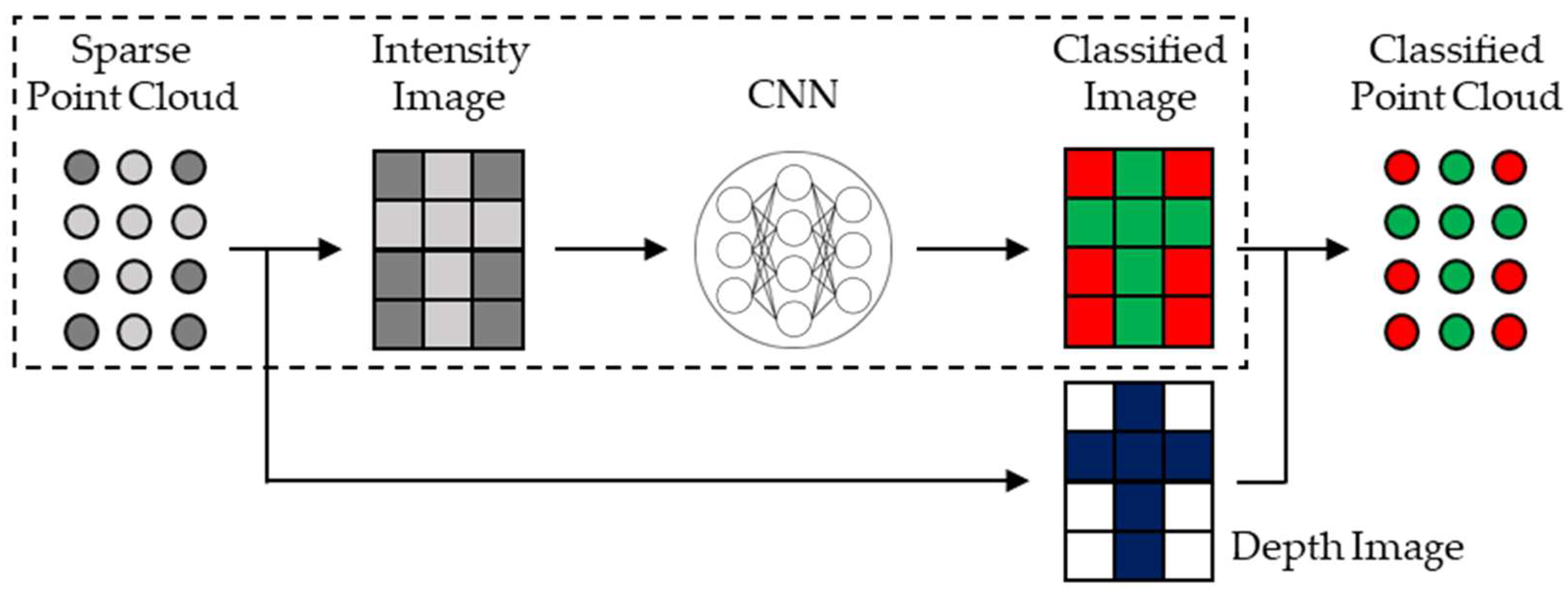
2.1. Dataset Preparation

The sparse point cloud used in this experiment was captured using a Velodyne Puck (VLP-16) LiDAR sensor mounted in front of a small vehicle tilted 45 degrees downward from horizontal. As shown in Figure 2, it was temporarily attached to the vehicle’s large windscreen, since there was no available space in front for a permanent installation. This enabled the scanning to obtain more ground surface points.
As shown in Figure 3, the scanning was carried out on roadways within the East Area of the Ookayama Campus, Tokyo Institute of Technology. The roads contained an assortment of road marking features but mainly consisted of lane lines and crosswalks. As a result, the target road markings were restricted to only these types.
The point clouds were then filtered to retain only points on the ground and in a portion in front of the vehicle, removing any unwanted points, such as vegetation and overhead structures, as illustrated in Figure 4. After which it was projected top-down into a 2D plane with a 1 cm square grid and average intensity as pixel values, yielding 2048 by 512-pixel BEV intensity images.
The intensity images were manually labeled into three classes to be used as training data for the CNN: ‘black’, which has no point cloud value, ‘road marking’, which is the target road marking, and ‘others’ which are all remaining pixels. A sample labeled image can be seen in Figure 4. These, along with the BEV intensity images, make up the training, validation, and testing datasets. Around 90% of all the processed images were used as training and validation data, which were further densified using the data augmentation method of multi-orientation flipping [20]. The remaining were used as testing data to assess the model performance in road marking extractions.
In this paper, the resulting predicted images will be dilated using a 3 × 3 kernel solely for visualization purposes. As shown in Figure 5, this is done to increase the interpretability of the results since the target features on the images are too small. Because of this, there may also be minor changes, but nothing significant enough to alter the outcome.

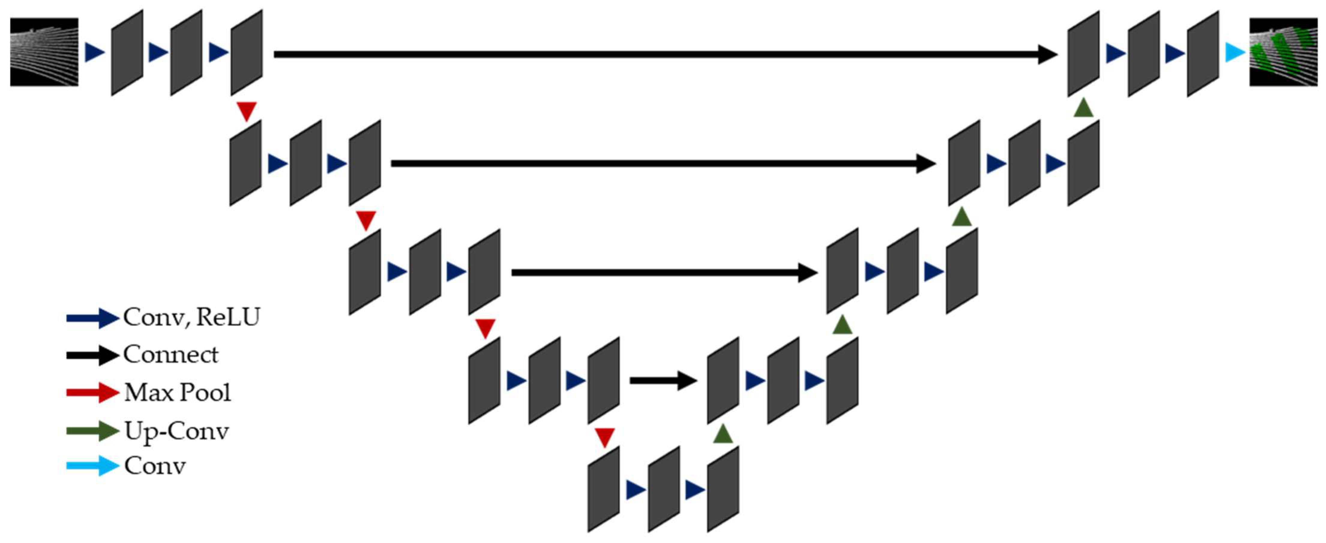
2.2. Convolutional Neural Network Models

To test for versatility, our proposed loss function will be applied to two differently structured convolutional neural networks, the popular and robust U-Net and a more lightweight fast-SCNN.
U-Net is a CNN that was originally designed for biomedical image segmentation. Its structure, as seen in Figure 6, consists of a symmetrically connected succession of convolution layers with pooling operators in the first half and upscaling operators in the latter half for better and more precise predictions [21]. It is a popular CNN model that is now widely used in varying scientific fields, including the extraction of road markings from point cloud-derived images. It has also surpassed other CNN models in terms of accuracy by achieving the highest F1 score, reaching up to 90% in extracting road markings [10,11,12,13,16].
FSCNN is a lighter CNN model that achieves real-time segmentation by utilizing popular techniques, such as pyramid pooling, inverted residual bottlenecks, and feature fusion, as seen in Figure 7 [22]. Recently, it has been explored for road marking extraction due to its suitability for low-cost applications, but its results were still inferior to U-Net’s under the same conditions. Nonetheless, it has been shown to achieve an F1-score of more than 70% at prediction speeds of 0.2 s [16,17].

2.3. Loss Functions

In deep learning, the loss function:
J W = k k ^ ,
is used to compute the difference between the predicted results ( k ^ ) and the actual labels k after going through an activation function. The resulting loss value is then minimized by backpropagating through the network layers to modify the network’s weights and biases through an optimization function:
W k + 1 = W k W k J W .
This is done by adding the gradient of the loss function in the opposite direction to the previous weights [18,19]. By applying the appropriate loss function when training, the CNN could be guided to make better predictions.
To begin with, a commonly used loss function is the cross-entropy loss,
C r o s s   E n t r o p y   L o s s = log P t   where   P t = p i f   k ^ = 1 1 p o t h e r w i s e .
It calculates the difference between two probability distributions for a set of events [23]. However, cross-entropy loss fails for imbalanced datasets, where certain classes greatly outnumber the other classes.
To address the issue of imbalanced datasets, predetermined class weights ( w ) can be introduced to cross-entropy loss:
Weighted Cross-Entropy Loss = w l o g P t .
where the weights are computed by taking the inverse ratio of the number of pixels in that class # s a m p l e s i multiplied by the total number of classes ( # c l a s s e s ) , with the total number of pixels in the image # s a m p l e s [24].
Class Weight = # s a m p l e s # c l a s s e s   ·   # s a m p l e s i  
Further improving the performance on imbalanced datasets, focal loss,
Weighed Focal Loss = w 1 P t γ l o g P t ,
introduced a modulating term 1 P t γ to penalize the contribution of easier classes and enabled the CNN model to concentrate more on learning harder classes [25]. The focal loss combined with class weights significantly boosts the capability of a CNN model in detecting sparse features in datasets with extreme class imbalance.
Another loss function that handles class imbalance well is dice loss,
Dice Loss = 1 2 T P + c 2 T P + F P + F N + c ,
Dice loss originates from the dice coefficient, or F1-score, evaluation metric modified with the addition of a smoothing constant to prevent gradient explosion. It makes use of the metric’s property as a harmonic mean to obtain a more accurate measure of the difference in correct overlaps even on harder features [26].
Leveraging this property, combo loss,
Combo Loss = α   M o d i f i e d w l o g P t + 1 α   1 2 T P 2 T P + F P + F N ,
takes the weighted sums of the dice loss and a modified cross-entropy loss as another approach to further improve the classification of poorly represented features [27]. However, it was demonstrated that using the proposed modified cross-entropy loss yielded the same F1-score as using the cross-entropy loss. Hence, in this paper, the non-modified version of cross-entropy will be used instead.
Returning to dice loss, a modulating term, in the form of an exponent factor 1 β , is introduced in focal dice loss,
Focal Dice Loss = 1 2 T P 2 T P + F P + F N 1 β .
Similar to focal loss, it aimed to direct dice loss into giving more focus to poorly segmented classes [28].
Our proposed loss function is a modified version of the combo loss,
Focal Combo Loss = α   w 1 P t γ l o g P t + 1 α   1 2 T P 2 T P + F P + F N 1 β ,
in which we take the weighted sum of the weighted focal combo loss and the focal dice loss, both developed to better focus on harder-to-classify features. This will be highly advantageous, given the scarcity of features in sparse point cloud-derived images.

2.4. Model Training

To speed up the training of multiple models, training was done on two computers. Tsubame 3.0, a supercomputer at the Tokyo Institute of Technology with four 16 GB GPU and 256 GB of RAM, was used to train U-Net models. A desktop computer with an 11 GB GPU and 48 GB of RAM was used to train fast-SCNN models.
Parameter limitations were set based on the computer with lower processing capacity to ensure a fair comparison. Because of these constraints, the batch size was limited to 16, and images for training and validation were downscaled to a quarter within the network. In addition, an Adam optimizer and a learning rate of 0.0001 was used.
To account for uncertainty, models were trained in three batches, each with fixed seeds, when training multiple models with changing loss functions. A total of 100 epochs were performed for each trial, using the model version at an epoch with the lowest loss value for road marking extraction.

3. Results

3.1. Generated Dataset

Table 1 lists the breakdown of pixels per class of the generated datasets used in the experiment. The overwhelming number of ‘black’ pixels makes it clear that there is an extreme class imbalance. Additionally, we can see that the target class ‘road marking’ is still considerably smaller than the ‘others’ class, which is already scant. This can have a significant impact on a CNN’s capability to correctly detect such sparse features.

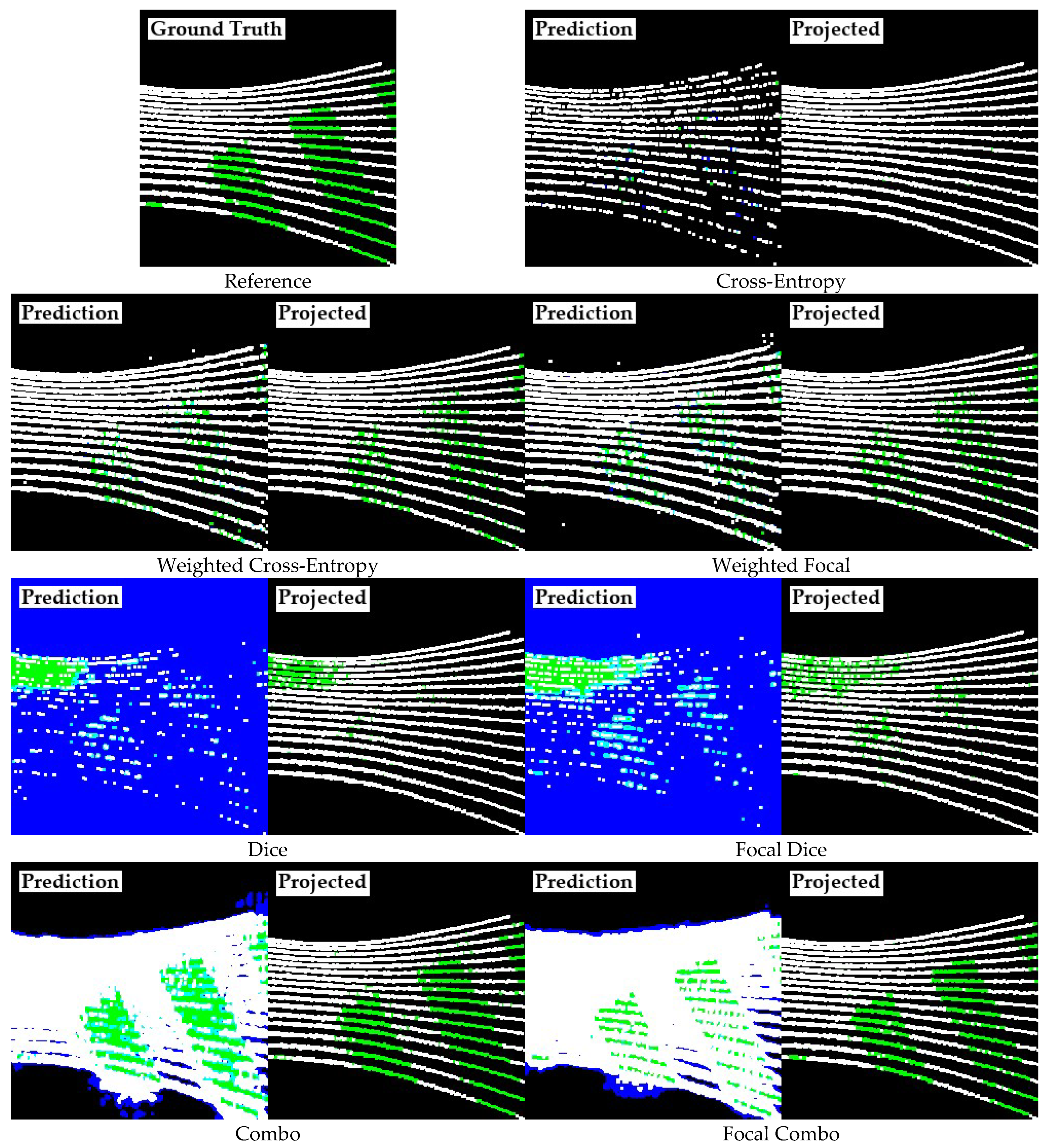
3.2. Resulting Images of Extracted Road Markings

Figure 8 and Figure 9 show the sample cropped predictions of road marking extractions using our proposed loss function, focal combo loss, in comparison to other related existing loss functions using the U-Net and fast-SCNN models, respectively. Projected versions of the classified images are shown alongside them, with only those with corresponding point cloud values retained.
Cross-entropy loss fails to classify road marking pixels for U-Net and does not classify anything at all for fast-SCNN. The addition of weights and a modulating term, in case of focal loss, proved to enhance model performance reflected by a partially visible depiction of the target road marking. For dice loss and focal dice loss, although they fared poorly, the results in the two models were completely different. In U-Net, dice and focal dice loss barely caught any road markings and showed a focused misclassification in a different region. In fast-SCNN, dice and focal dice loss were able to correctly classify all road markings but overreached and included a large portion of the surrounding pixels. Nonetheless, only combo loss and our proposed focal combo loss produced good representations of road markings. However, it is important to notice that only our proposed focal combo loss prediction achieved a cleaner result when only pixels with point cloud values were retained.

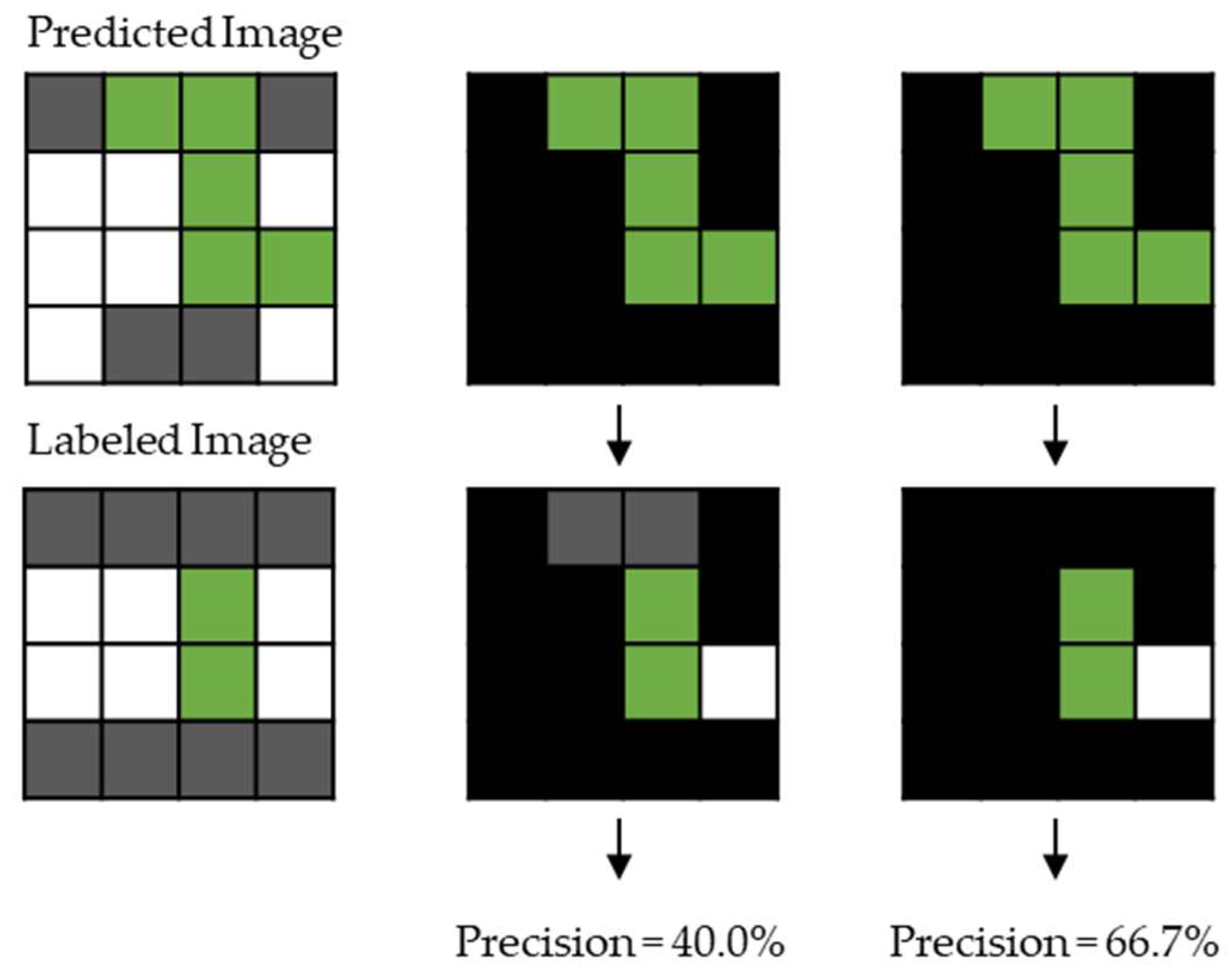
3.3. Assessment Criteria

Road marking extraction was evaluated through the following criteria obtained from the calculated confusion matrix between the predicted and actual image: recall, precision, F1-score, and intersection-over-union (IoU), as shown in Equations (11)–(14). Recall means that pixels in the reference image correspond correctly to those in the predicted image. Precision, on the other hand, means that pixels in the predicted image correspond correctly to those in the reference image. High values in both of those criteria indicate that the extraction was successful. Taking both into account, the F1-score, also known as the dice coefficient, is the harmonic mean of precision and recall. The harmonic mean tends to favor smaller values; it is a reliable criterion for uneven precision and recall. As a final measure, the IoU, also known as the Jaccard index, is also included. It divides the correctly overlapping pixels by the union of the reference and the prediction, making the resulting value nearer the minimum of precision and recall [29]. Table 2 and Table 3 shows the initial assessment results based on these criteria.
R e c a l l = T r u e   P o s i t i v e T r u e   P o s i t i v e + F a l s e   N e g a t i v e   ,
P r e c i s i o n = T r u e   P o s i t i v e T r u e   P o s i t i v e   +   F a l s e   P o s i t i v e   ,
F 1 s c o r e = 2 × P r e c i s i o n × R e c a l l P r e c i s i o n + R e c a l l ,
IoU = T r u e   P o s i t i v e T r u e   P o s i t i v e + F a l s e   P o s i t i v e + F a l s e   N e g a t i v e  
For the succeeding tables, rows with a gray background contain our results and values in bold refer to the highest mean score in the corresponding evaluation criteria.

3.4. Assessment after ‘Black’ Pixel Omission

As a special property of sparse point cloud-derived images, misclassifications in the ‘black’ pixels can be omitted in the assessment computations, as these pixels correspond to no value when projected as a point cloud, as shown in Figure 10. Since ‘black’ pixels occupy most of the images, this has a significant impact on the evaluation.
In Table 4 and Table 5, after removing misclassifications in the ‘black’ pixels, we can see a tremendous increase in the evaluation results. Our proposed loss function, focal combo loss, achieved the highest mean F1-score in both models, outperforming all other loss functions. Combo loss came close, but focal combo loss proved to be more reliable by having the smallest uncertainty and the highest minimum value for both the F1-score and IoU.

3.5. Analyzing the Weighted Sum Combinations

The parameters γ and β, which were used in the focal combo loss, were derived from the γ and β of the best-performing weighted focal loss and focal dice loss. Parameter α, on the contrary, determines which of the loss functions in the weighted sum had the strongest influence on achieving the best road marking extraction results. From Table 6 and Table 7, we can derive that focal dice loss had a greater influence on both models.

4. Discussion

We now compare the results of our proposed focal combo loss to those of existing methods on road marking extractions from point cloud-derived BEV images using CNNS, after comparing them to the results of related existing functions.
Figure 11 clearly shows that our proposed loss function, focal combo loss, still manages to outperform existing CNN methods that have been used for road marking extractions on point cloud-derived BEV images. Table 8 backs this up by showing that it has the highest F1-score and IoU among the competition. More importantly, we can see that a lighter model, fast-SCNN with a focal combo loss, could best even the other methods that used the U-Net model.
Overall, we can see that the inability of focal combo loss to produce high precision values compared to cross-entropy loss is a limiting factor. This means that in its attempt to focus on harder features, it tends to prioritize minimizing the difference to the actual labeled image, even if it exaggerates predictions at the target class’s bounds. Furthermore, it can be seen that it is unnecessarily the better-performing loss function that should be given more weight in the weighted sum. Focal dice loss performed far less than the weighted focal loss, but having a stronger influence on it caused the best performance in our proposed focal combo loss.
In addition, as mentioned in the overview of the methodology, in Figure 12 the extracted road markings can be combined with depth images to generate classified sparse point clouds as an extension. Figure 8 shows that this procedure can produce promising results for both CNN models trained with focal combo loss. However, it is clear that U-Net provides better geometry than fast-SCNN, but given that fast-SCNN has shown prediction speeds of 0.2 s, it shows potential for achieving real-time road marking extraction.

5. Conclusions

In this work, we proposed a modified loss function, focal combo loss, to improve the automatic extraction of road markings from sparse mobile point cloud-derived BEV images using CNNs. It is an attempt to provide expensive alternatives by using data obtained from lower-cost LiDAR sensors rather than survey-grade LiDAR sensors typically installed on a MMS. This can be a practical approach for tasks involving multiple and frequent deployments and involving road markings, such as road monitoring and HD map updates.
Focal combo loss was able to outperform all related existing loss functions as well as existing CNN methods used for road marking extraction on three fronts. First is accuracy, with U-Net and fast-SCNN achieving the highest mean F1-score values of 85.4 and 68.9, respectively. Second is reliability, factoring in uncertainty values of ±1.1 and ±4.2 and yielding minimum values of 84.3 and 64.7, respectively, which are the highest among all other minima. The third and final front is versatility, which is reflected in the previous two fronts by consistently being the best in both models.
In future work, we intend to implement our method on more complex road environments with more diverse road markings. Modifications of the other components of the deep learning framework will also be explored, such as the modification of the CNN structure and the training procedure, to further improve road marking extractions on sparse point cloud-derived images. Other feature extraction applications, such as targeting vehicles, pedestrians, and cyclists from a different projection perspective, will also be investigated. This could provide additional support for advocating the use of low-cost sensors for mobile mapping.

Author Contributions

Conceptualization, M.L.R.L.; Methodology, M.L.R.L.; Formal analysis, M.L.R.L.; Writing—original draft, M.L.R.L.; Writing—review & editing, M.L.R.L.; Supervision, M.M. All authors have read and agreed to the published version of the manuscript.

Funding

The research was supported by Tokyo Institute of Technology’s WISE Program for Super Smart Society. A special thanks go out to Zongdian Li of Sakageuchi-Tran Laboratory, Department of Electrical and Electronics Engineering, Tokyo Institute of Technology, who assisted and provided expertise during the data collection.

Data Availability Statement

The data presented in this study are available on request from the corresponding author.

Conflicts of Interest

The authors declare no conflict of interest.

References

  1. Ma, L.; Li, Y.; Li, J.; Wang, C.; Wang, R.; Chapman, M. Mobile Laser Scanned Point-Clouds for Road Object Detection and Extraction: A Review. Remote Sens. 2018, 10, 1531. [Google Scholar] [CrossRef] [Green Version]
  2. Chiang, K.; Zeng, J.; Tsai, M.; Darweesh, M.; Chen, P.; Wang, C. Bending the Curve of HD Maps Production for Autonomous Vehicle Applications in Taiwan. IEEE J. Sel. Top. Appl. Earth Obs. Remote Sens. 2022, 15, 8346–8359. [Google Scholar] [CrossRef]
  3. Seif, H.; Hu, X. Autonomous Driving in the iCity–HD Maps as a Key Challenge of the Automotive Industry. Engineering 2016, 2, 159–162. [Google Scholar] [CrossRef] [Green Version]
  4. Liu, R.; Wang, J.; Zhang, B. High Definition Map for Automated Driving: Overview and Analysis. J. Navig. 2020, 73, 324–341. [Google Scholar] [CrossRef]
  5. Kashani, A.; Olsen, M.; Parrish, C.; Wilson, N. A Review of LIDAR Radiometric Processing: From Ad Hoc Intensity Correction to Rigorous Radiometric Calibration. Sensors 2015, 15, 28099–28128. [Google Scholar] [CrossRef] [PubMed] [Green Version]
  6. Chen, S.; Liu, B.; Feng, C.; Vallespi-Gonzales, C.; Wellington, C. 3D Point Cloud Processing and Learning for Autonomous Driving. IEEE Signal Process. Mag. 2021, 38, 68–86. [Google Scholar] [CrossRef]
  7. Cheng, M.; Zhang, H.; Wang, C.; Li, J. Extraction and Classification of Road Markings Using Mobile Laser Scanning Point Clouds. IEEE J. Sel. Top. Appl. Earth Obs. Remote Sens. 2017, 10, 1182–1196. [Google Scholar] [CrossRef]
  8. Pan, Y.; Yang, B.; Li, S.; Yang, H.; Dong, Z.; Yang, X. Automatic Road Marking Extraction, Classification and Vectorization from Mobile Laser Scanning Data. Int. Arch. Photogramm. Remote Sens. Spat. Inf. Sci. 2019, XLII-2/W13, 1089–1096. [Google Scholar] [CrossRef] [Green Version]
  9. Soilan, M.; Riveiro, B.; Martinez-Sanchez, J.; Arias, P. Segmentation and Classification of Road Markings using MLS Data. ISPRS J. Photogramm. Remote Sens. 2017, 123, 94–103. [Google Scholar] [CrossRef]
  10. Wen, C.; Sun, X.; Li, J.; Wang, C.; Guo, Y.; Habib, A. A Deep Learning Framework for Road Marking Extraction, Classification and Completion from Mobile Laser Scanning Point Clouds. ISPRS J. Photogramm. Remote Sens. 2019, 14, 178–192. [Google Scholar] [CrossRef]
  11. Lagahit, M.; Tseng, Y. Using Deep Learning to Digitize Road Arrow Markings from LIDAR Point Cloud Derived Images. Int. Arch. Photogramm. Remote Sens. Spat. Inf. Sci. 2020, 43, 123–129. [Google Scholar] [CrossRef]
  12. Lagahit, M.; Tseng, Y. Road Marking Extraction and Classification from Mobile LIDAR Point Clouds Derived Imagery using Transfer Learning. J. Photogramm. Remote Sens. 2021, 26, 127–141. [Google Scholar]
  13. Ma, L.; Li, Y.; Li, J.; Yu, Y.; Junior, J.M.; Goncalves, W.N.; Chapman, M. Capsule-Based Networks for Road Marking Extraction and Classification from Mobile LiDAR Point Clouds. IEEE Trans. Intell. Transp. Syst. 2021, 22, 1981–1995. [Google Scholar] [CrossRef]
  14. Elhashash, M.; Albanwan, H.; Qin, R. A Review of Mobile Mapping Systems: From Sensors to Applications. Sensors 2022, 22, 4262. [Google Scholar] [CrossRef]
  15. Masiero, A.; Fissore, F.; Guarnieerri, A.; Vettore, A.; Coppa, U. Development and Initial Assessment of a Low Cost Mobile Mapping System. R3 Geomat. Res. Results Rev. 2020, 1246, 116–128. [Google Scholar]
  16. Lagahit, M.; Matsuoka, M. Boosting U-Net with Focal Loss for Road Marking Classification on Sparse Mobile LIDAR Point Cloud Derived Images. ISPRS Ann. Photogramm. Remote Sens. Spat. Inf. Sci. 2022, 5, 33–38. [Google Scholar] [CrossRef]
  17. Lagahit, M.; Matsuoka, M. Exploring FSCNN + Focal Loss: A Faster Alternative for Road Marking Classification on Mobile LIDAR Sparse Point Cloud Derived Images. In Proceedings of the 2022 IEEE International Geoscience and Remote Sensing Symposium, Kuala Lumpur, Malaysia, 17–22 July 2022; pp. 3135–3138. [Google Scholar]
  18. Jadon, S. A Survey of Loss Functions for Semantic Segmentation. In Proceedings of the 2020 IEEE Conference on Computational Intelligence in Bioinformatics and Computational Biology, Vina del Mar, Chile, 27–29 October 2020. [Google Scholar]
  19. Wang, Q.; Ma, Y.; Zhao, K.; Tian, Y. A Comprehensive Survey of Loss Functions in Machine Learning. Ann. Data Sci. 2022, 9, 187–212. [Google Scholar] [CrossRef]
  20. Shorten, C.; Khoshgoftaar, T. A survey on Image Data Augmentation for Deep learning. J. Big Data 2019, 6, 60. [Google Scholar] [CrossRef]
  21. Ronneberger, O.; Fischer, P.; Brox, T. U-Net: Convolutional Networks for biomedical Image Segmentation. arXiv 2015, arXiv:1505.04597. [Google Scholar]
  22. Poudel, R.; Liwicki, S.; Cipolla, R. Fast-SCNN: Fast Semantic Segmentation Network. arXiv 2019, arXiv:1902.04502. [Google Scholar]
  23. Kohonen, T.; Barna, G.; Chrisley, R. Statistical Pattern Recognition with Neural Networks: Benchmarking Studies. In Proceedings of the IEEE 1988 International Conference on Neural Networks, San Diego, CA, USA, 24–27 July 1988; Volume 1, pp. 61–68. [Google Scholar]
  24. Picek, S.; Heuser, A.; Jovic, A.; Bhasin, S.; Regazzoni, F. The Curse of Class Imbalance and Conflicting Metrics with Side-Channel Evaluations. IACR Trans. Cryptogr. Hardw. Embed. Syst. 2019, 1, 209–237. [Google Scholar]
  25. Lin, T.; Goyal, P.; Girshick, R.; He, K.; Dollar, P. Focal Loss for Dense Object Detection. In Proceedings of the IEEE International Conference on Computer Vision (ICCV), Venice, Italy, 22–29 October 2017; pp. 2980–2988. [Google Scholar]
  26. Sudre, C.; Li, W.; Vercauteren, T.; Ourselin, S.; Cardoso, M.J. Generalized Dice Overlap as a Deep Learning Loss Function for highly Unbalanced Segmentations. In Deep Learning in Medical Image Analysis and Multimodal Learning for Clinical Decision Support; Lecture Notes in Computer Science; Springer: Cham, Switzerland, 2017; Volume 10553, pp. 240–248. [Google Scholar]
  27. Taghanaki, S.; Zheng, Y.; Zhou, S.K.; Georgescu, B.; Sharma, P.; Xu, D.; Comaniciu, D.; Hamarneh, G. Combo Loss: Handling Input and Output Imbalance in Multi-Organ Segmentation. Comput. Med. Imaging Graph. 2019, 75, 24–33. [Google Scholar] [CrossRef] [PubMed] [Green Version]
  28. Wang, P.; Chung, A.C. Focal Dice Loss and Image Dilation for Brain Tumor Segmentation. In Deep Learning in Medical Image Analysis and Multimodal Learning for Clinical Decision Support; Lecture Notes in Computer Science; Springer: Cham, Switzerland, 2018; Volume 11045, pp. 119–127. [Google Scholar]
  29. Tharwat, A. Classification Assessment Methods. Appl. Comput. Inform. 2018, 17, 168–192. [Google Scholar] [CrossRef]
Figure 1. Road marking extraction procedure.
Remotesensing 15 00597 g001
Figure 2. The small vehicle used for LiDAR scanning, with the LiDAR sensor encircled in red.
Remotesensing 15 00597 g002
Figure 3. Encircled in red are the scanning location (left) taken from the Tokyo Tech website and road marking types visible in the area (right) taken from Google Earth.
Remotesensing 15 00597 g003
Figure 4. Sample sparse point cloud before (left) and after (right) filtering.
Remotesensing 15 00597 g004
Figure 5. Sample image of the dataset (top) and dilated counterpart for visualization (bottom). The red square indicates the location of the detected road marking.
Remotesensing 15 00597 g005
Figure 6. U-Net structure.
Remotesensing 15 00597 g006
Figure 7. Fast-SCNN structure.
Remotesensing 15 00597 g007
Figure 8. Sample prediction results and projected counterparts using U-Net.
Remotesensing 15 00597 g008
Figure 9. Sample prediction results and projected counterparts using fast-SCNN.
Remotesensing 15 00597 g009
Figure 10. Rethinking assessment computation for sparse point cloud-derived images.
Remotesensing 15 00597 g010
Figure 11. Sample prediction results using existing methods in road markings and their projected counterparts.
Remotesensing 15 00597 g011aRemotesensing 15 00597 g011b
Figure 12. Sample generated classified sparse point cloud.
Remotesensing 15 00597 g012
Table 1. Dataset statistics.
DatasetNumber of ImagesNumber of Pixels per Class
BlackOthersRoad Marking
Training100099.03%0.88%0.09%
Validation10099.04%0.76%0.20%
Testing 10099.03%0.94%0.03%
Table 2. Initial results for U-Net in (%) for the road marking class.
LossRecallPrecisionF1-ScoreIoU
[23]Cross Entropy7.3 ± 4.567.2 ± 6.112.8 ± 7.66.9 ± 4.2
[24]Weighted Cross Entropy46.9 ± 5.442.7 ± 5.244.3 ± 0.628.4 ± 0.5
[25]Weighted Focal (γ = 1)52.5 ± 6.037.9 ± 5.744.0 ± 5.928.3 ± 4.9
[26]Dice3.0 ± 5.01.2 ± 1.40.7 ± 0.80.3 ± 0.4
[28]Focal Dice (β = 3)8.3 ± 14.15.4 ± 6.21.3 ± 1.80.7 ± 0.9
[27]Combo (α = 0.50)96.2 ± 2.710.5 ± 2.218.8 ± 3.410.4 ± 2.1
Focal Combo
(γ = 1, β = 3, α = 0.25)
95.3 ± 1.39.9 ± 0.818.0 ± 1.39.9 ± 0.8
Table 3. Initial results for fast-SCNN in (%) for the road marking class.
LossRecallPrecisionF1-ScoreIoU
[23]Cross Entropy0.0 ± 0.0------0.0 ± 0.0
[24]Weighted Cross Entropy55.4 ± 12.26.4 ± 0.611.4 ± 1.06.0 ± 0.6
[25]Weighted Focal (γ = 5)52.7 ± 8.85.9 ± 0.410.5 ± 0.75.6 ± 0.4
[26]Dice56.8 ± 46.93.3 ± 1.04.6 ± 1.22.4 ± 0.6
[28]Focal Dice (β = 1.5)57.4 ± 48.43.4 ± 0.74.8 ± 2.52.5 ± 1.3
[27]Combo (α = 0.25)61.5 ± 10.45.2 ± 0.49.6 ± 0.85.0 ± 0.4
Focal Combo
(γ = 5, β = 1.5, α = 0.25)
66.6 ± 1.75.5 ± 0.810.1 ± 1.35.3 ± 0.7
Table 4. Results after the ‘black’ pixel omission for U-Net in (%) for the road marking class.
LossRecallPrecisionF1-ScoreIoU
[23]Cross Entropy7.3 ± 4.597.1 ± 0.213.3 ± 8.025.3 ± 15.2
[24]Weighted Cross Entropy46.9 ± 5.495.6 ± 0.562.8 ± 4.750.7 ± 4.9
[25]Weighted Focal (γ = 1)52.5 ± 6.094.3 ± 1.767.3 ± 55.25.2 ± 7.9
[26]Dice3.0 ± 5.02.2 ± 1.91.8 ± 2.70.9 ± 1.4
[28]Focal Dice (β = 3)8.3 ± 14.114.3 ± 16.73.9 ± 6.32.1 ± 3.3
[27]Combo (α = 0.50)96.2 ± 2.776.4 ± 6.784.9 ± 3.173.9 ± 4.6
Focal Combo
(γ = 1, β = 3, α = 0.25)
95.3 ± 1.377.4 ± 2.785.4 ± 1.174.5 ± 1.7
Table 5. Results after the ‘black’ pixel omission for fast-SCNN in (%) for the road marking class.
LossRecallPrecisionF1-ScoreIoU
[23]Cross Entropy0.0 ± 0.0---------
[24]Weighted Cross Entropy55.4 ± 12.280.9 ± 10.664.6 ± 6.548.2 ± 6.9
[25]Weighted Focal (γ = 5)52.7 ± 8.885.2 ± 3.364.9 ± 6.748.7 ± 7.7
[26]Dice56.8 ± 46.941.3 ± 5.237.7 ± 28.726.3 ± 19.3
[28]Focal Dice (β = 1.5)57.4 ± 48.443.4 ± 10.040.0 ± 32.928.8 ± 23.7
[27]Combo (α = 0.25)61.5 ± 10.478.2 ± 4.168.6 ± 7.653.7 ± 6.8
Focal Combo
(γ = 5, β = 1.5, α = 0.25)
66.6 ± 1.971.4 ± 6.968.9 ± 4.252.9 ± 4.8
Table 6. Results of analyzing parameter α for U-Net in (%) for the road marking class.
αRecallPrecisionF1-ScoreIoU
0.2595.3 ± 1.377.4 ± 2.785.4 ± 1.174.5 ± 1.7
0.50 66.7 ± 19.379.0 ± 5.170.9 ± 8.155.3 ± 10.1
0.75 23.4 ± 10.585.7 ± 7.836.2 ± 13.422.7 ± 10.5
Table 7. Results of analyzing parameter α for fast-SCNN in (%) for the road marking class.
αRecallPrecisionF1-ScoreIoU
0.2566.6 ± 1.971.4 ± 6.968.9 ± 4.252.9 ± 4.8
0.50 68.0 ± 3.969.0 ± 10.768.0 ± 4.451.9 ± 5.1
0.7560.0 ± 21.770.5 ± 10.261.9 ± 11.145.7 ± 11.3
Table 8. Results in comparison to existing methods in (%) for the road marking class.
MethodRecallPrecisionF1-ScoreIoU
[11]U-Net + Cross Entropy 7.3 ± 4.597.1 ± 0.213.3 ± 8.025.3 ± 15.2
[12]U-Net + Cross Entropy
(Transfer Learning)
6.7 ± 1.197.9 ± 0.912.5 ± 2.030.2 ± 1.5
[13]U-Net + Weighted Focal 52.5 ± 6.094.3 ± 1.767.3 ± 55.25.2 ± 7.9
[10]U-Net + IoU8.4 ± 14.5------2.4 ± 4.2
U-Net + Focal Combo95.3 ± 1.377.4 ± 2.785.4 ± 1.174.5 ± 1.7
[14]Fast-SCNN + Weighted Focal 52.7 ± 8.885.2 ± 3.364.9 ± 6.748.7 ± 7.7
Fast-SCNN + Focal Combo66.6 ± 1.771.4 ± 6.968.9 ± 4.252.9 ± 4.8
Disclaimer/Publisher’s Note: The statements, opinions and data contained in all publications are solely those of the individual author(s) and contributor(s) and not of MDPI and/or the editor(s). MDPI and/or the editor(s) disclaim responsibility for any injury to people or property resulting from any ideas, methods, instructions or products referred to in the content.

