Article

Spectral Characteristics of the Dynamic World Land Cover Classification

1
Lamont-Doherty Earth Observatory, Columbia University, New York, NY 10027, USA
2
Department of Geography, San Diego State University, San Diego, CA 92182, USA
*
Author to whom correspondence should be addressed.
Remote Sens. 2023, 15(3), 575; https://doi.org/10.3390/rs15030575
Submission received: 31 December 2022 / Revised: 12 January 2023 / Accepted: 16 January 2023 / Published: 18 January 2023
(This article belongs to the Special Issue Feature Papers for Section Biogeosciences Remote Sensing)

Abstract

:
The Dynamic World product is a discrete land cover classification of Sentinel 2 reflectance imagery that is global in extent, retrospective to 2015, and updated continuously in near real time. The classifier is trained on a stratified random sample of 20,000 hand-labeled 5 × 5 km Sentinel 2 tiles spanning 14 biomes globally. Since the training data are based on visual interpretation of image composites by both expert and non-expert annotators, without explicit spectral properties specified in the class definitions, the spectral characteristics of the classes are not obvious. The objective of this study is to quantify the physical distinctions among the land cover classes by characterizing the spectral properties of the range of reflectance present within each of the Dynamic World classes over a variety of landscapes. This is achieved by comparing both the eight-class probability feature space (excluding snow) and the maximum probability class assignment (label) distributions to continuous land cover fraction estimates derived from a globally standardized spectral mixture model. Standardized substrate, vegetation, and dark (SVD) endmembers are used to unmix nine Sentinel 2 reflectance tiles from nine spectral diversity hotspots for comparison between the SVD land cover fraction continua and the Dynamic World class probability continua and class assignments. The variance partition for the class probability feature spaces indicates that eight of these nine hotspots are effectively five-dimensional to 95% of variance. Class probability feature spaces of the hotspots all show a tetrahedral form with probability continua spanning multiple classes. Comparison of SVD land cover fraction distributions with maximum probability class assignments (labels) and probability feature space distributions reveal a clear distinction between (1) physically and spectrally heterogeneous biomes characterized by continuous gradations in vegetation density, substrate albedo, and structural shadow fractions, and (2) more homogeneous biomes characterized by closed canopy vegetation (forest) or negligible vegetation cover (e.g., desert, water). Due to the ubiquity of spectrally heterogeneous biomes worldwide, the class probability feature space adds considerable value to the Dynamic World maximum probability class labels by offering users the opportunity to depict inherently gradational heterogeneous landscapes otherwise not generally offered with other discrete thematic classifications.

1. Introduction

The Dynamic World product (www.dynamicworld.app (accessed on 11 January 2023)) is a discrete land cover classification of Sentinel 2 reflectance imagery that is global in extent, retrospective to 2015, and updated continuously in near real time. The classifier, based on a fully convolutional neural network (FCNN) trained on labeled image polygons (as opposed to individual pixel spectra), incorporates both spatial and spectral information [1]. The classifier is trained on a stratified random sample of 20,000 hand-labeled 5 × 5 km Sentinel 2 tiles spanning 14 biomes globally [1]. The output of the classifier is a 9-class probability vector and a maximum probability class assignment for each 10 × 10 m Sentinel 2 pixel. Since the training data are based on visual interpretation of image composites by both expert and non-expert annotators, without explicit spectral properties specified in the class definitions, the spectral characteristics of the resulting classes are not obvious. Any constraints on the spectral characteristics of the Dynamic World classes that can be inferred from comparison to the input Sentinel 2 reflectance data could inform use of the classification as an input to physical process models.
In contrast to discrete land cover classifications based on categorical assignment, continuous field land cover maps are generally based on directly interpretable physical properties of the land surface inferred from observed reflectance spectra (derived from radiance measurements). Vegetation abundance maps derived from spectral indices (e.g., NDVI) are a common example (e.g., [2]). Implicit in the continuous field model is the understanding that the physical property of interest may vary continuously over a range of spatial scales spanning the pixel size of the imaging sensor. In contrast to maps based on a single spectral index of a specific physical property, continuous field spectral mixture models (discussed in detail in [3]) are based on the understanding that multiple spectrally distinct endmember materials, possibly occurring at spatial scales finer than sensor pixel resolution, may contribute to a spectrally mixed radiance measurement. Spectral mixture models mathematically simulate the spatial aggregation of the upwelling radiance field within a single-pixel field of view. Inversion of a spectral mixture model provides simultaneous per-pixel estimates of the relative areal abundance (fractions) of each endmember material potentially present within the field of view of the pixel [4,5,6,7]. As a result, endmember fraction maps can simultaneously accommodate continuous gradients in multiple physical properties associated with a multitude of land cover types.
The objective of this study is to characterize the spectral properties of the range of reflectance present within each of the Dynamic World classes (except snow, which was not included with the classification product for any of the nine hotspots used here) over a variety of landscapes to constrain the physical distinctions among the land cover classes. By comparing both the eight-class probability feature space and the maximum probability class assignment (label) distributions to continuous land cover fraction estimates derived from a globally standardized spectral mixture model, we investigate the relationship between the class probability feature space produced by the Dynamic World classifier and the Sentinel 2 spectral feature space represented by the spectral mixture model. The generative physical conditions underlying the spectral feature space on which the mixture model is based can then be mapped onto the class probability feature space to quantify the physical and spectral properties of each class in the context of the Sentinel 2 reflectance. Understanding the correspondence of the land cover classes to the purely pixel-level spectral properties of the mixture model may also allow for inference on the contribution of the spatial context to the classification result, since any cases where spectrally inseparable land cover classes are correctly (or incorrectly) distinguished by the classifier must presumably be a result of spatial context rather than spectral properties alone.
In this study, we use a linear mixture model to represent physical and spectral characteristics of a diversity of landscapes as a compositional and spectral continuum. Analyses of the spectral dimensionality and feature space topology of global compilations of broadband imagery reveal a striking consistency in the spectral diversity of most ice-free landscapes [8,9,10,11]. The spectral mixture model that is inverted to provide spectral endmember fraction estimates is based on the understanding that the most spectrally distinct types of materials found in most ice-free landscapes are photosynthetic vegetation, rock and soil substrate, and water. In addition to the subpixel areal abundance of these generic spectral endmembers, the spectral mixture model can also accommodate variations in substrate albedo and subpixel shadow. Since low-albedo substrates (e.g., black soil, fresh basalt) and deep shadows are often spectrally indistinguishable from deep clear water by optical sensors, they can be combined into a single dark spectral endmember. As explained in detail below, a global compilation of 80,000,000 11-band Sentinel 2 spectra, collected from a compilation of 80 spectral diversity hotspots worldwide [12], can be modeled by the generalized three-component Substrate, Vegetation, Dark (SVD) linear spectral mixture model with <6% misfit for 99% of spectra (<4% for 95%).

2. Materials and Methods

2.1. Data

To span as diverse a range of land cover and landscapes as possible with a reasonable number of examples, we focused on a set of spectral diversity hotspots. Each hotspot spans multiple biomes and climatic zones, as well as development intensities. We selected 9 such hotspots from a larger collection of 140 chosen as part of a global analysis of the Sentinel 2 spectral feature space [12,13]. The full collection of 140 hotspots contains many anomalous landscapes, containing spectrally uncommon materials such as open pit mines and tailing ponds, lithium evaporite ponds, carbonate dune fields, extensive greenhouse complexes, tropical icecaps, and solar reflector arrays. We selected bounding SVD endmembers from a subset of 80 of these 140 hotspots, chosen to be broadly representative of the most common natural and human-modified landscapes. In this down-selection, we specifically excluded snow- and ice-covered areas (for reasons explained below), evaporite basins, reef and shallow marine environments, and other areas unlikely to fall within the range of the nine classes of the Dynamic World product. The 80 hotspots used for endmember selection are intended to maximize the diversity of non-polar biomes used to construct the composite feature space from which the bounding SVD endmembers were selected.
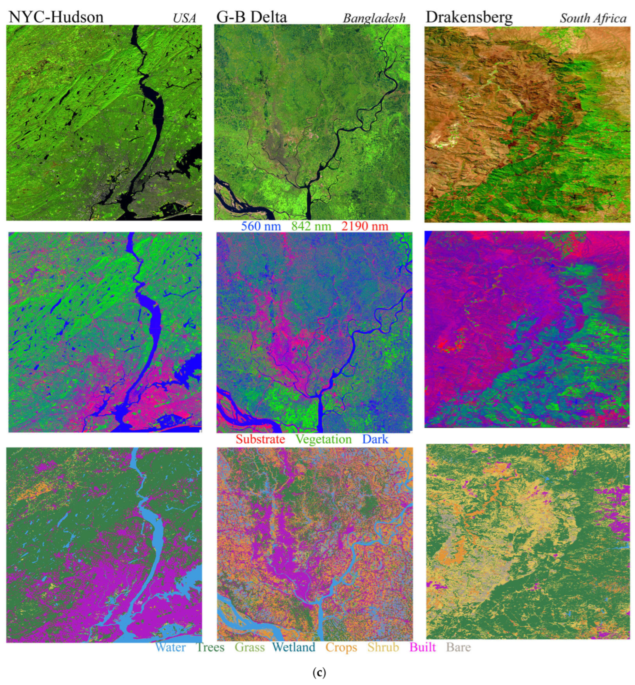
Five of the nine hotspots chosen were incorporated as full (110 × 110 km) Sentinel 2 exoatmospheric reflectance tiles. For four hotspots, sub-tiles were used because they occur at swath edges with less than full tile coverage or contain large areas of ocean. All dates were chosen to maximize spectral diversity and solar illumination and minimize cloud cover. Only one example (Andes-Amazon) contained a small amount of visible cloud cover, which was masked in the Dynamic World product. The nine hotspots chosen for the analysis are shown in Figure 1a–c as Visible/NearIR/ShortwaveIR composites, SVD landcover fraction composites, and Dynamic World maximum probability class maps for the specific Sentinel 2 acquisition date used. For each hotspot tile chosen, the Dynamic World probability feature space and maximum probability class (label) for the same day were acquired from Google Earth Engine. Brief descriptions of each are provided below and Table 1.
Laguna Mountains–Sonoran Desert: The Laguna-Sonoran hotspot in southern California spans the near-coastal western slope of the Laguna mountains, the forested range top, and the Anza-Borrego section of the Sonoran Desert in the rain shadow to the east. Upslope from the near-coastal suburban developments, the land cover transitions from chaparral to open woodland at the 1200 m range top. Woodland rapidly grades into desert scrub in the rain shadow downslope to the Salton Trough below sea level.
San Joaquin Valley: The San Joaquin hotspot in the southern part of the Great Central Valley of California is one of most diverse and productive agricultural basins on Earth. The broad, flat valley bottom hosts rich soils supportive of industrial-scale production of diverse, high-value crops. This cropland-dominated landscape is interspersed with human settlements, most notably the city of Fresno in the north-central portion of the tile. The distinct southwest portion of the scene is reflective of soil and crop differences linked to the northern end of the now-dry Tulare Lake and associated drainages.
Coast Ranges–Transverse Ranges: The Coast-Transverse hotspot at the southern end of the California Riviera spans the intersection of the Coast Ranges trending northward and the Transverse ranges trending eastward. The agriculturally dominated Santa Ynez valley occupies the space between the Coast and Transverse ranges in the northwest corner of this scene. Notably, the abrupt reorientation of the coastline from N-S to E-W orientation (at Point Conception) occurs at the transition between the Southwestern and Central Coastal floristic regions of California, and the Northern California Current and Southern California Current marine ecoregions. The complex convergence of multiple biogeographic factors establishing this spectral diversity hotspot gives this site global significance for biodiversity and conservation [14].
Andean Altiplano–Amazon Basin: The Andes-Amazon hotspot spans a climatic gradient encompassing 5 biomes ranging from >5500 to <500 m elevation. The Altiplano is composed of ice-capped mountains and semi-arid scrubland descending into the Amazon basin, primarily composed of biodiverse, closed canopy, humid tropical forest.
Mauna Kea–Kohala watersheds: The Mauna Kea-Kohala hotspot on the island of Hawaii spans multiple biomes along multiple elevation gradients along a ridge extending from Mauna Kea summit (~4500 m) to sea level. A rain shadow extends southeastward from the humid tropical forests and farms on the northeast slopes over extensive grassland flanking the ridge down to the arid scrublands and lava flows on the southwestern slope of the volcano. The forest preserves in the Kohala watershed on the northern slope of the ridge are considered a biodiversity hotspot.
Nilgiri Mountains, Western Ghats: The Western Ghats hotspot is near the southernmost extent of the west coast of India. From the semi-arid 1000 m Deccan Plateau in the northeast, over the 3000 m Nilgiri Mountains, down to near sea level on the west coastal plain, this hotspot spans at least 4 biomes and contains the Nilgiri biosphere reserve.
New York City–Hudson River Valley and Highlands: The NYC-Hudson hotspot in the northeastern USA contains a diversity of urban, suburban, peri-urban, and rural development amid temperate deciduous forest. Climatically and ecologically, it is the least diverse of the hotspots, but the most diverse in terms of developed land cover.
Ganges–Brahmaputra Delta: The G-B Delta hotspot in Bangladesh spans a variety of terrains and hydrologic settings on the largest, most populous delta on Earth. The tropical megacity of Dhaka is surrounded by a diverse agricultural mosaic interspersed with anthropogenically forested embankments, villages, and agricultural fields supporting one to three crops per year, with an agricultural diversity approaching that of the San Joaquin Valley hotspot.
Transvaal Drakensberg: The Drakensberg hotspot spans the Southern African Central Plateau and the westernmost section of the Great African Escarpment. Highveld and bushveld environments on the plateau at ~1000 m elevation rise to >1500 m forests on the escarpment before plummeting to <50 m on the lowveld savannah to the east.
For each of the nine hotspots, the eight-class probability vector and maximum probability class assignment (label) of the Dynamic World product were extracted using Google Earth Engine for the date corresponding to the Sentinel 2 surface reflectance product obtained from the European Space Agency Copernicus Open-Access Hub (https://scihub.copernicus.eu/ (accessed on 1 April 2022)). All Dynamic World classifications were extracted from Google Earth Engine at the native (10 m) resolution and UTM zone of the Sentinel 2 tile using the Export.image.toDrive() function in Earth Engine.
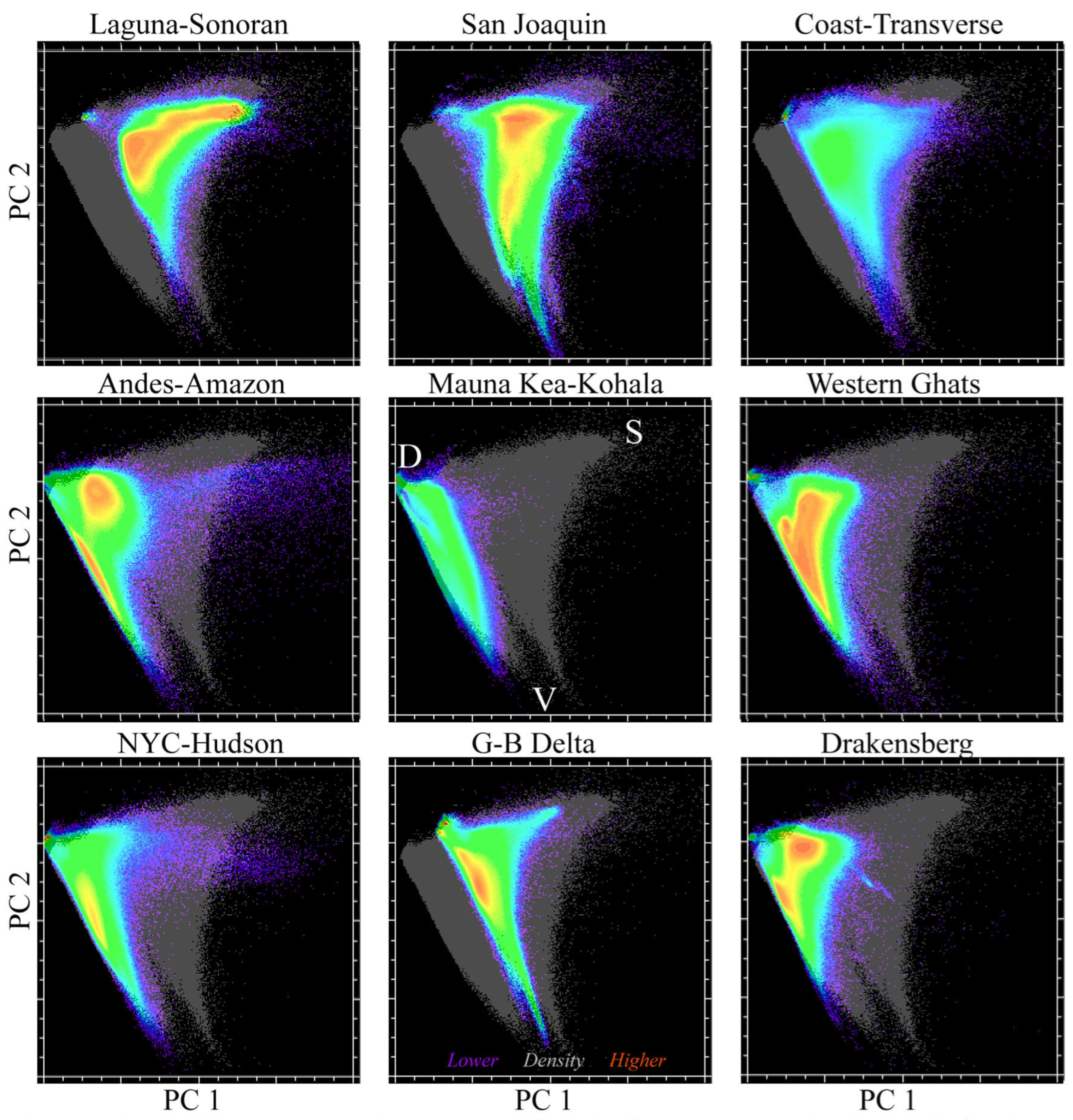
Spectral feature spaces for both the 80- and 9-hotspot composites were rendered as orthogonal projections of the 3 low-order principal component distributions (PCs), as shown in Figure 2. In both cases, the feature spaces are effectively 2-dimensional (2D), with the SVD plane of PCs 1 and 2 accounting for >95% of the total variance of the full 10D space (bands 1–8, 11, 12). The SVD spectral endmembers identified from the 3D feature space of the 80-hotspot composite bound both the 80- and 9-hotspot spaces. Figure 3 shows the PC1-2 SVD spaces of each individual hotspot projected onto the silhouette of the 9-hotspot PC1-2 space for comparison. Each example shows the spectral continuum spanning a range of substrate albedos and tapering as the vegetation fraction increases approaching the vegetation endmember. Two internal vegetation endmembers are apparent in the 9-hotspot space. These correspond to open canopy vegetation (e.g., savannah) mixing with underlying substrate (soil and non-photosynthetic vegetation) and closed canopy vegetation (e.g., forest) mixing with subpixel inter-crown shadow. Within the larger and more spectrally diverse 80-hotspot space, both mixing trends are encompassed within a single substrate–vegetation mixing continuum, incorporating a greater diversity of biomes, substrates, and vegetation types.

2.2. Methods

The SVD endmembers bounding the 80-hotspot composite were used as standardized global endmembers to unmix both composites. In this study, the global composite was unmixed only to assess model validity and obtain the RMS misfit distribution (discussed below). All SVD fraction comparisons in this study were based on the 9 hotspots only.
The 3-endmember linear spectral mixture model is given explicitly as a set of 10 band-specific mixing equations. Since the number of mixing equations exceeded the number of unknown fractions, the system was overdetermined, allowing for inversion by minimization of model misfit.
FSE1 + FVE1 + FDE1         R1
.          .            .           =     .
.          .            .                 .
FSE10 + FVE10 + FDE10         R10
In matrix notation:
R = FE + ε
where E is the 3-column matrix of 10-band endmember vectors, R is the observed reflectance vector to be modeled, FS|V|D is the vector of endmember fractions to be estimated, and ε is the model misfit to be minimized by the inversion. In addition, a unit sum constraint equation was added to the model to urge the fractions to sum to 1. As in earlier such analyses using Landsat [8,9,10] and MODIS [11], the least squares solution, F = (ETE)1ET R [15], for the SVD endmember fraction estimates, yielded a stable result with fractions well-bounded [0, 1]. Model validity was assessed by multiplying the estimated SVD fractions with the SVD endmember spectra to forward model the observed mixed spectra. The distribution of root mean square (RMS) misfit between the observed and modeled spectra for the 80-hotspot composite had <6% misfit for >99% of 80,000,000 Sentinel 2 spectra (and <4% for 95%). The same global SVD endmembers were used to unmix the 9-hotspot composite. All subsequent comparisons used the SVD fractions estimated from inversion of the SVD mixture model for the 9-hotspot composite. The misfit distribution of the 9-hotspot composite was virtually identical to that of the 80-hotspot composite.
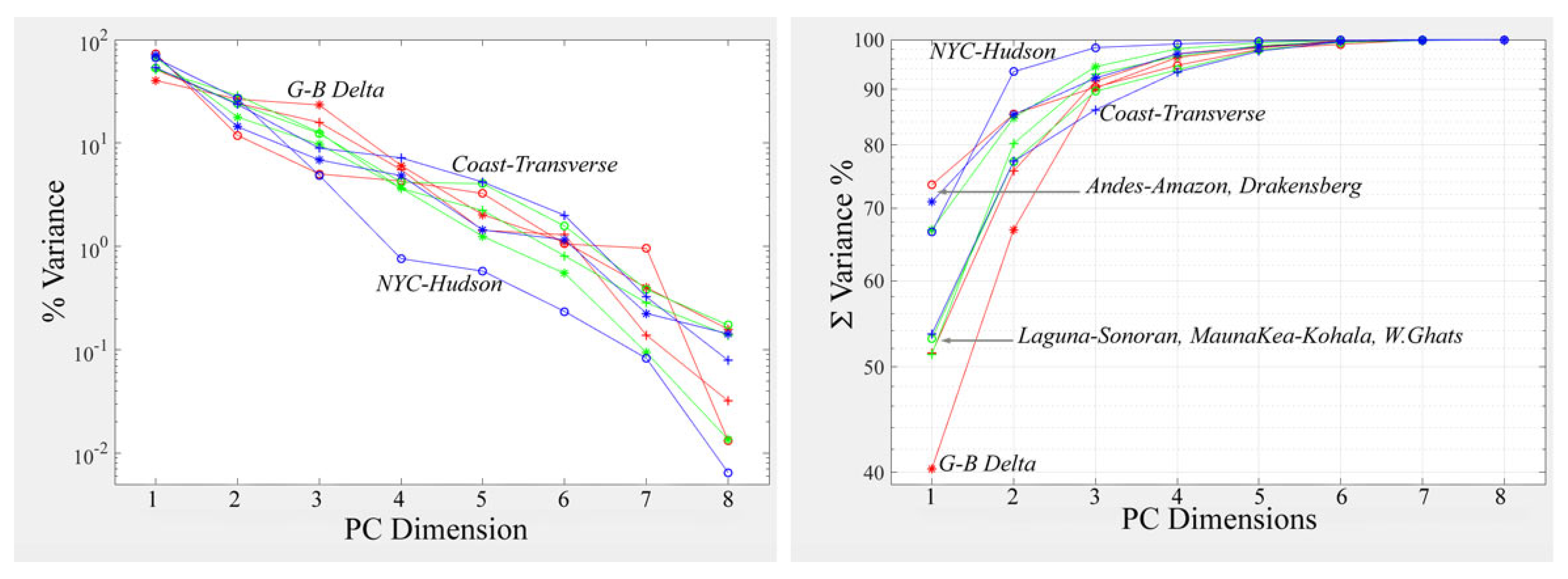
As with the Sentinel 2 spectral feature spaces, the dimensionality and topology of the Dynamic World class probability feature space were quantified by principal component analysis. For both the spectral and probability feature spaces, both covariance- and correlation-based transforms were compared, with nearly identical results. Subsequent analysis used the covariance-based transforms. Figure 4 shows the variance partition of each of the 9 hotspot probability feature spaces, as given by the normalized eigenvalues of each 9D feature space. All probability feature spaces, except NYC-Hudson, are effectively 5D, requiring 5 dimensions to account for >95% of the total feature space variance. NYC-Hudson is effectively 3D as it is dominated by a smaller number of classes.
For comparison to the PC-based class probability feature space, we also rendered low-dimensional projections of the full 8D feature space using the Uniform Manifold Approximation and Projection (UMAP) algorithm [16]. UMAP is a nonlinear algorithm that seeks to preserve the essential topological structure of a high-dimensional dataset while embedding it in a low-dimensional space. For this analysis, UMAP was computed in Python using the scikit-learn.manifold implementation (version 0.24.2).
UMAP manifolds were computed for both 2D and 3D projections with default hyperparameter settings and neighborhood scales ranging from 5 to 500. All projections yielded similar topologies and class distributions, although larger neighborhood values produced more compact projections with greater distinctions among classes.
Spectral separability matrices were computed for all class pairs using full 10-band Sentinel 2 reflectance spectra distributions from each hotspot. We used transformed divergence (TD) [17] to quantify spectral separability to avoid the pathologic convergence properties of other separability metrics [18]. As implemented here, TD ranged from 0 for identically overlapping classes to 2 for completely separable classes. The often-quoted interpretation of [0–1.5 ≤ 1.5–1.9 ≤ 1.9–2.0]~[Poor ≤ Moderate ≤ Good] separability appears to be apocryphal, as we can find no study to explicitly substantiate it. However, in an empirical study of crop classifications with 1 to 6 classes, the authors of [19] found that 90% classification accuracy spanned a TD range from ~1.125 to 2.0 with a mean of 1.9, for which the accuracy distribution spanned a range from 83% to 95%.

3. Results

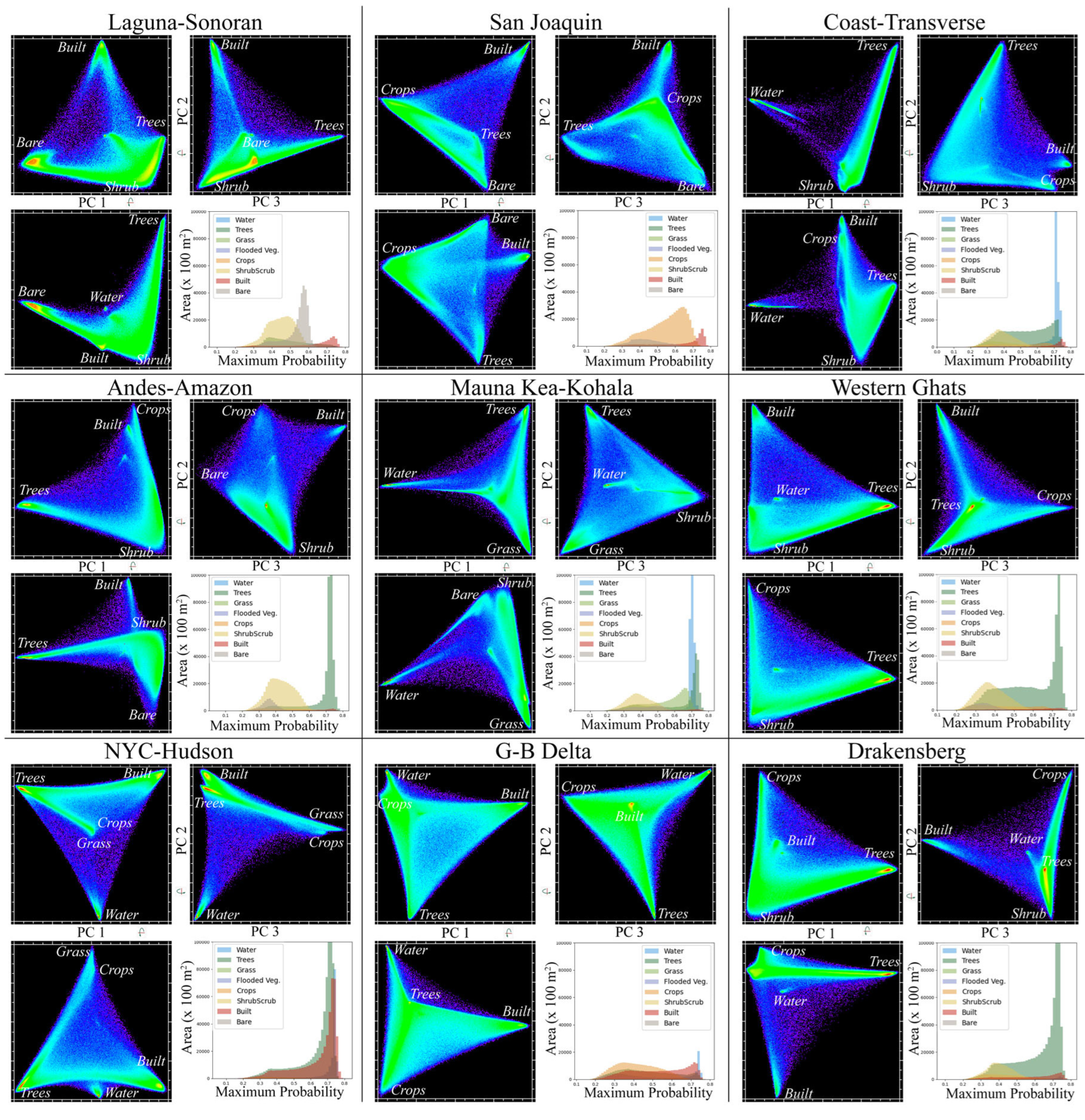
The class probability feature spaces of all nine hotspots share a similar topology. Figure 5 shows orthogonal projections of the three low-order PCs of each as density-shaded bivariate distributions. All are characterized by tetrahedral topology, in which the maximum probability of each class membership occupies a distinct apex with probability continua spanning the tetrahedral simplex bounding the apices. The resemblance of the probability feature spaces to the spectral feature spaces is clear, as is the absence of distinct clusters within the probability feature spaces. Higher densities between apices indicate probability continua between classes. Histograms of the corresponding maximum probability class assignments show a clear contrast between classes with modes at higher (>~0.7) maximum probability (e.g., Trees, Water) and classes with modes at lower (<~0.5) maximum probability (e.g., Shrub, Bare).
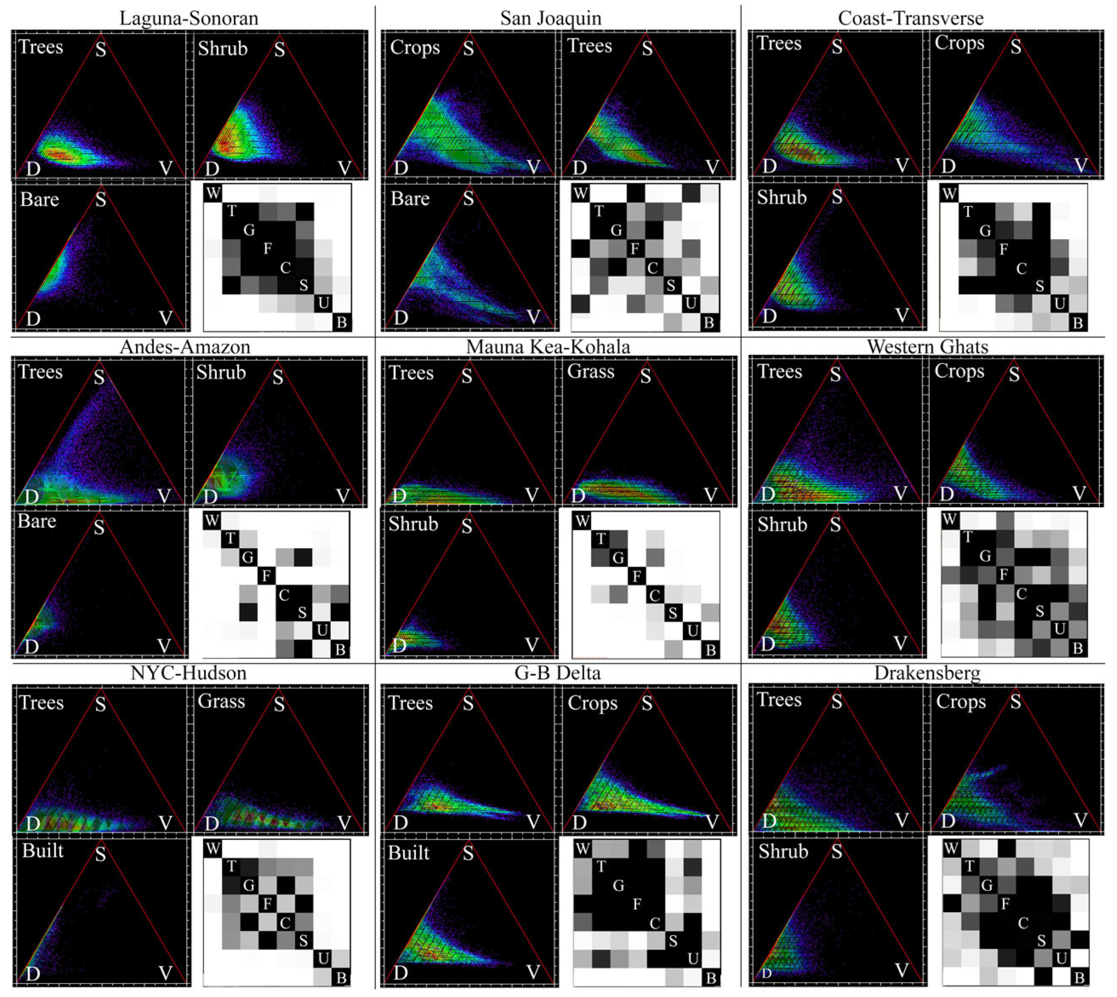
Spectral characteristics of each land cover class can be quantified by mapping maximum probability class assignments (labels) onto their pixels’ corresponding SVD fraction distributions. Figure 6 shows SVD fraction distributions on ternary diagrams for the three primary classes (indicated by the apices of the low-order PCs shown in Figure 5) of each hotspot. Each trivariate distribution of SVD fractions shows the continua of spectral characteristics of each class for each hotspot. The continuity of the SVD fraction distributions reflects the continuous land cover gradients that dominate most of the hotspots. All the spectral continua have a similar form with a range of substrate albedos on the S-D binary mixing line, extending toward increasing vegetation fractions. Distributions attaining higher vegetation fractions (e.g., Trees, Crops) show a clear tapering of the distribution with an increasing vegetation fraction. This tapering is a result of increasing canopy closure reducing the range of substrate albedo and shadowing. Spectral separability matrices for each hotspot show more statistically separable class pairs as lighter shades of gray. Darker class pair matrix cells represent class pairs that are less statistically separable and correspond to classes with greater overlap in their SVD distributions. Variations in the structure of the spectral separability matrices indicate differences in the spectral properties of class assignments in different landscapes.
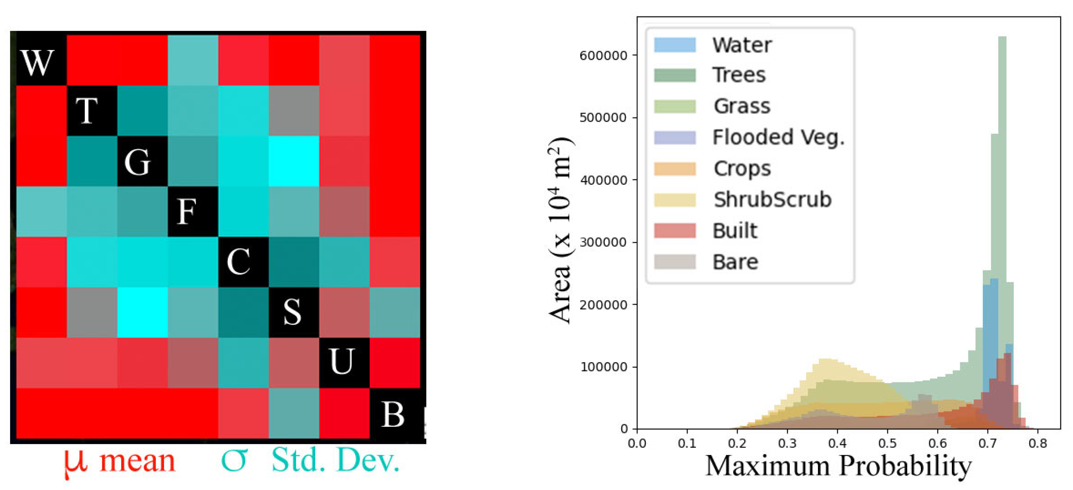
Aggregating the maximum probability distributions and spectral separability matrices shows both the consistency and variability of class assignment among the nine hotspots. Figure 7 shows the mean and standard deviation of aggregated TD scores for all class pairs over the nine hotspots. The Water and Bare classes showed the highest mean separability (>1.9, red) from other classes, with the lowest variability among hotspots. Each showed more variable separability (cyan) with one other class (Water:Flooded, Bare:Shrub). The Built class (U) showed moderately high (>1.8) separability with all classes except Crops (1.67). Aggregate maximum probability histograms for class assignments showed the same distinctions as individual hotspot distributions, with Water and Trees having strongly skewed distributions with a higher modal probability (>0.7) and Shrub having a more platykurtic distribution with a lower modal probability (<0.4). Crops had a nearly uniform distribution with maximum probabilities ranging from 0.2 to 0.7. The Bare class had a bimodal distribution with modes at ~0.36 and ~0.58, reflecting lower probability despite the generally high separability with all but the Shrub (S) class.
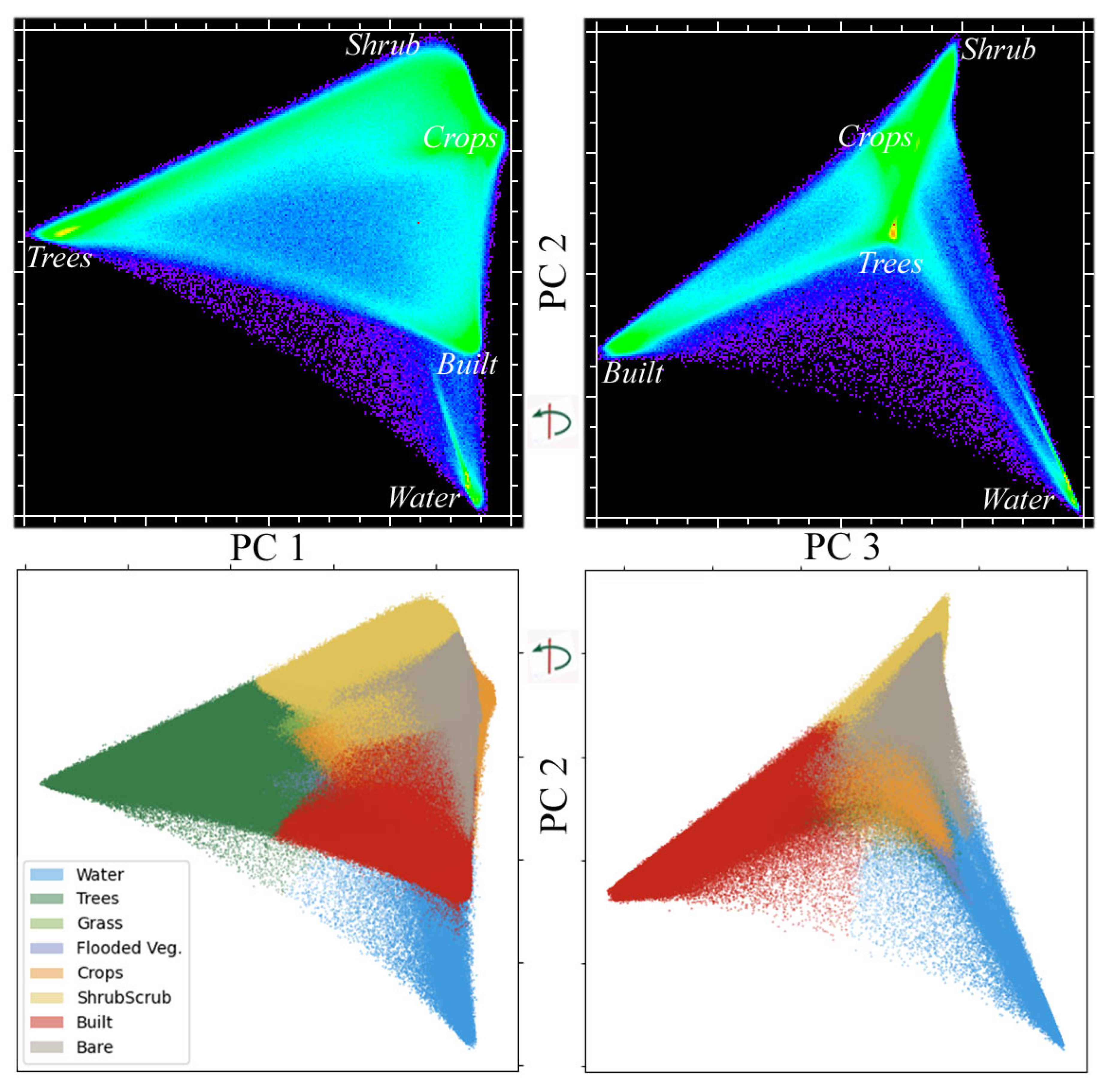
The aggregate probability feature space of all nine hotspots retained the tetrahedral topology of the individual hotspot feature spaces. Figure 8 shows orthogonal projections of the PC1-3 feature space as density-shaded bivariate distributions and maximum probability class assignments. Mapping class assignments (labels) onto the probability distributions clearly showed the class decision boundaries as discontinuities within the probability feature space. The variance partition among the low-order PCs of the probability feature space was less skewed than the variance partition of the spectral feature spaces shown in Figure 2, indicating the higher dimensionality of the probability feature space. The variance partition given by the principal component transform reflects both the number and amplitude of class probability vectors in the probability feature space. For this reason, the PC projection of the feature space emphasizes the probability continua within the higher dimensional space. In contrast, a projection of the feature space that preserves the local manifold structure rather than maximizing variance provides an alternative depiction of the 9D probability feature space. The 2D projection given by the Uniform Manifold Approximation and Projection (UMAP) algorithm (Figure 9) more clearly distinguished the continuum among the Trees, Shrub, and Crops classes from the more distinct Water, Bare, and Built classes. The Grass class was divided between the center of the Trees–Shrub–Crops continuum and a separate cluster. The separate grass cluster corresponds to the Mauna Kea–Kohala hotspot as a homogeneous pasture on low-albedo basaltic soil on the upper flanks of the volcano. This anomalously dark substrate is also apparent on the ternary diagrams in Figure 6.

4. Discussion

4.1. The SVD Model: Why It Works

The SVD model is the most parsimonious continuous field model capable of accurately representing the reflectance of the (evaporite- and ice-free) land cover continuum. Analysis of 43,000,000 MODIS spectra spanning 9 1200 × 1200 km spectrally diverse transitional landscapes worldwide found >99% of variance in a 3D feature space, in which >95% of spectra could be fit by the SVD model with <5% RMS misfit at a 500 m resolution [11]. Similar studies of global Landsat compilations found similar spectral dimensionality and SVD topology, in which >98% of Landsat spectra could be fit with <5% RMS misfit at a 30 m resolution for >100,000,000 spectra [9,10]. Even spectrally diverse compilations of AVIRIS hyperspectral imagery reveal SVD topologies in the low-order dimensions [20,21], albeit with higher overall spectral dimensionality reflective of the greater information content recoverable with greater spectral resolution.
The ubiquity of the SVD feature space topology over a diversity of geographies and range of spatial scales reflects the consistent nature of terrestrial biomes in which most ice-free landscapes can be considered a continuum of substrate surfaces of varying suitability to support a continuum of vegetation communities, while intersecting local water tables to form a variety of standing and flowing water bodies. Terrain slope relative to illumination results in a continuum of solar flux densities and shadows, while a continuum of vegetation structure, height, and density superimposes a continuum of finer-scale shadow on the landscape. The near orthogonality of the SVD reflectance spectra makes them well-suited to a parsimonious spectral mixture model that is sufficiently linear (at meter to kilometer scales) to allow for stable inversion with relatively small misfit in a wide variety of landscapes. Hence, the fundamental physical properties of land cover (chemical composition, morphology, and scale) are adequately captured by aggregate optical reflectance to produce a ternary continuum of physical/spectral properties that can represent the global variety of evaporite- and ice-free biomes. The spectral mixture model can also be extended to cryospheric environments, although the spectral diversity of the snow–firn–ice continuum and the structural morphology of glaciers and ice sheets introduces considerable complexity relative to the SVD model for ice-free landscapes [22,23]. We note that the Dynamic World product did not include a probability layer for snow and ice in any of the nine hotspots used in this study. Mountain glaciers and high-elevation snow cover present in the Andes-Amazon hotspot are classified as water (as are the few clouds present).

4.2. The Dynamic World Class Probability Continuum

When the Dynamic World class probability feature space is rendered based on variance (via low-order PCs), which is sensitive to both number and amplitude of probability vectors, the 3D topology is consistently tetrahedral (in compositionally diverse settings), both for individual hotspots and in composites. This continuum of class probabilities is a manifestation of the continua of substrates and vegetation communities in the diverse transitional landscapes of the nine hotspots, as well as a continuum of view and illumination geometries manifest in the imaging process.
The variety of distributions of maximum probability for different classes reflects the different characteristics of Sentinel 2 reflectance within different land cover classes across different landscapes, as well as the consistency in interpretation reflected in the confusion matrices in [1]. More homogeneous and compositionally consistent classes such as Water and Trees (forest) have clearly defined modes at high probabilities with long lower tails extending to the Bare–Shrub continuum that encompasses most (7 of 14) non-forested terrestrial biomes. The fractal nature of human settlements [24] and the interspersed nature of the peri-urban interface results in a land cover continuum spanning the gradient from urban to suburban to peri-urban to rural [25]. This continuum is also reflected in the class probability feature space. Crops are manifest as a continuum within the Tree–Shrub–Bare continuum because the Crops class itself encompasses a continuum between fallow fields and mature crops. The lower probabilities of the upper tail of the Shrub class, and the bimodal nature of the Bare class, reflect the difficulty of interpretation (and discrimination) of these classes within the land cover continuum.
While the PC feature space depicts the probability continua as tetrahedral, the UMAP manifolds preserve local structure lost in the variance-based PC projections. In the UMAP manifold shown in Figure 9, the Trees–Shrub–Crops continuum is more clearly distinguished from the Built, Bare, and Water limbs. Grass on the upper slopes of the Mauna Kea–Kohala hotspot appears as a separate cluster because it is superimposed on the anomalously low-albedo basalt-derived soils of the upper slopes of Mauna Kea volcano. The small amount of Grass class in the other hotspots maps onto the center of the Trees–Scrub–Crops continuum, as would be expected.

4.3. Spectral Characteristics and Physical Properties of the Dynamic World Classes

The overlapping SVD distributions and generally low spectral separability of several of the classes in most of the hotspots (Figure 6) are completely consistent with the continuous nature of the class probability feature space, and the widely variable accuracies reported in [1]. This is to be expected considering the spectral continua that characterize most biomes in diverse landscapes, such as those of the spectral diversity hotspots. Since the tiles used for the Dynamic World accuracy assessment presumably contain a combination of heterogeneous transitional landscapes, such as those in the spectral diversity hotspots used in this analysis, and more spectrally homogeneous landscapes (e.g., boreal and tropical forests, deserts), the aggregate accuracies reported in [1] probably reflect a combination of lower accuracies in heterogeneous landscapes and higher accuracies in more homogeneous landscapes. This type of setting-dependent accuracy is unavoidable in discrete thematic classification and enhances the value of the class probability vectors provided with the Dynamic World product. Rendering the maximum probability class assignment maps as shaded surfaces (as illustrated in [1]) is a novel way to incorporate this important information into visual depictions. Alternatively, in landscapes dominated by three or fewer classes, continuous probability gradients could be depicted using R, G, and B color composites. Overall, the class probability vectors add considerable value to the Dynamic World maximum probability class labels by offering users the opportunity to use the classifier outputs to depict inherently gradational landscapes otherwise not generally offered with other discrete thematic classifications.

4.4. Information Content and Spatial Context

To borrow from the continuous field model of land cover, the concept of a continuum can be applied to a typology of discrete classification models themselves. One way to envision land cover classifications regards the source of information content. At one end of such a continuum could be purely spectral models, which consider only the spectral feature space of individual geographic pixels when assigning class membership—without regard to spatial context. This encompasses majority of thematic classifications traditionally used with remotely sensed data. At the opposite end of this continuum could be purely spatial models, which rely primarily on spatial context (e.g., segmentation) with little regard to spectral information (beyond spatial brightness variations that provide some part of the spatial context). Both endmember models fail to use some part of the information content of spectral imaging data. Object-based classifications (and CNNs) can be seen as a hybrid, using adjacency and spectral similarity together to assign membership in discrete objects with discrete class membership, while unavoidably introducing additional sources of uncertainty and error propagation.
Viewed in this light, one way of framing the purpose of introducing spatial convolution into a classification is the extraction of additional information from spatial context which is not present in the pixel-level spectra alone, specifically, the adjacency and even possibly texture of multiple spectrally similar pixels into spatial patterns analogous to objects in object-based classifications. However, the extraction of this information also introduces a fundamental tradeoff, which can be manifest as an increase in class overlap (decrease in spectral separability) when measured by statistics based on pixel-level reflectance spectra (or mixture fractions). Here, we intentionally used distributions of pixel-level SVD fractions to contrast the pixelwise and spatial convolution approaches. To extend this, one avenue for future work might consider a fusion of approaches in which spatial convolution and subsequent learning operators are performed on the SVD fraction images, rather than the reflectance images. This might improve model interpretability (and possibly reduce computational burden when training the NN). The low misfit of the global SVD model suggests that this could still capture the preponderance (>95% on average) of the spectral variance present in the reflectance images and potentially mitigate overfitting by effectively serving as a pre-model noise filter.
Finally, we take this opportunity to speculate about the potential of deep learning for spatiotemporal classification of image time series. Seasonality (in the form of vegetation phenology, solar illumination geometry, soil moisture, and snow cover) and even interannual trends provide a complementary source of information that can supplement the spectral characteristics of different land cover types. Whereas Convolutional Neural Networks can incorporate persistent spatial patterns (scale-limited) into the classification process, time series forecasting approaches (e.g., Recurrent Neural Networks and Encoder–Decoder models) have the potential to identify temporal consistencies (duration-limited) in pixel time series. The attention mechanism model is of particular interest for the potential information content of the attention weights themselves, as well as the interpretability of its results. It is beyond the scope of this study to speculate on the potential for explicitly combining convolutional and attention mechanism models, but the combined use of spectral and temporal mixture models for phenology mapping suggests that spatial and temporal information content can be applied, either in series or parallel, to land cover mapping and classification.

5. Conclusions

  • We used a continuous, pixelwise, physical land cover model to characterize a discrete, spatially convolved, statistical land cover classification.
  • SVD land cover fractions provided simple, physically meaningful quantification of Dynamic World class similarity and difference.
  • Continuous tetrahedral simplices consistently emerged in the Dynamic World class probability space.
  • Topology-preserving UMAP manifolds embedded from the Dynamic World probability space revealed further topological structure not obvious from PC feature spaces.
  • SVD land cover fractions provided interpretable physical context to the spatio-spectral information used by FCNN-based models.

Author Contributions

Conceptualization, C.S. and D.S.; methodology, C.S. and D.S.; writing and editing, C.S. and D.S. All authors have read and agreed to the published version of the manuscript.

Funding

D.S. gratefully acknowledges funding from the USDA NIFA Sustainable Agroecosystems program (Grant # 2022-67019-36397), the NASA Land-Cover/Land Use Change program (Grant # NNH21ZDA001N-LCLUC), the NASA Remote Sensing of Water Quality program (Grant # 80NSSC22K0907), and the NSF Signals in the Soil program (Award # 2226649). C.S. acknowledges the support of the endowment of the Lamont Doherty Earth Observatory.

Data Availability Statement

All data used in this study are publicly available from the web portal indicated in the manuscript text.

Acknowledgments

D.S. thanks Jean Allen and Rachel Wegener for assistance in developing code to export the Dynamic World class images from Google Earth Engine.

Conflicts of Interest

The authors declare no conflict of interest.

References

  1. Brown, C.F.; Brumby, S.P.; Guzder-Williams, B.; Birch, T.; Hyde, S.B.; Mazzariello, J.; Czerwinski, W.; Pasquarella, V.J.; Haertel, R.; Ilyushchenko, S.; et al. Dynamic World, Near Real-Time Global 10 m Land Use Land Cover Mapping. Sci. Data 2022, 9, 251. [Google Scholar] [CrossRef]
  2. Zeng, Y.; Hao, D.; Huete, A.; Dechant, B.; Berry, J.; Chen, J.M.; Joiner, J.; Frankenberg, C.; Bond-Lamberty, B.; Ryu, Y.; et al. Optical Vegetation Indices for Monitoring Terrestrial Ecosystems Globally. Nat. Rev. Earth Environ. 2022, 3, 477–493. [Google Scholar] [CrossRef]
  3. Adams, J.B.; Gillespie, A.R. Remote Sensing of Landscapes with Spectral Images: A Physical Modeling Approach; Cambridge University Press: Cambridge, UK, 2006. [Google Scholar]
  4. Adams, J.B.; Smith, M.O.; Johnson, P.E. Spectral Mixture Modeling: A New Analysis of Rock and Soil Types at the Viking Lander 1 Site. J. Geophys. Res. Solid Earth 1986, 91, 8098–8112. [Google Scholar] [CrossRef]
  5. Smith, M.O.; Ustin, S.L.; Adams, J.B.; Gillespie, A.R. Vegetation in Deserts: I. A Regional Measure of Abundance from Multispectral Images. Remote Sens. Environ. 1990, 31, 1–26. [Google Scholar] [CrossRef]
  6. Gillespie, A.; Smith, M.; Adams, J.; Willis, S.; Fischer, A.; Sabol, D. Interpretation of Residual Images: Spectral Mixture Analysis of AVIRIS Images, Owens Valley, California. In Proceedings of the Second Airborne Visible/Infrared Imaging Spectrometer (AVIRIS) Workshop, Pasadena, CA, USA, 4–5 June 1990; NASA: Pasadena, CA, USA, 1990; pp. 243–270. [Google Scholar]
  7. Johnson, P.E.; Smith, M.O.; Taylor-George, S.; Adams, J.B. A Semiempirical Method for Analysis of the Reflectance Spectra of Binary Mineral Mixtures. J. Geophys. Res. Solid Earth 1983, 88, 3557–3561. [Google Scholar] [CrossRef]
  8. Small, C. The Landsat ETM+ Spectral Mixing Space. Remote Sens. Environ. 2004, 93, 1–17. [Google Scholar] [CrossRef]
  9. Small, C.; Milesi, C. Multi-Scale Standardized Spectral Mixture Models. Remote Sens. Environ. 2013, 136, 442–454. [Google Scholar] [CrossRef] [Green Version]
  10. Sousa, D.; Small, C. Global Cross-Calibration of Landsat Spectral Mixture Models. Remote Sens. Environ. 2017, 192, 139–149. [Google Scholar] [CrossRef] [Green Version]
  11. Sousa, D.; Small, C. Globally Standardized MODIS Spectral Mixture Models. Remote Sens. Lett. 2019, 10, 1018–1027. [Google Scholar] [CrossRef]
  12. Small, C.; Sousa, D. The Sentinel 2 MSI Spectral Mixing Space. Remote Sens. 2022, 14, 5748. [Google Scholar] [CrossRef]
  13. Sousa, D.; Small, C. Joint Characterization of Sentinel-2 Reflectance: Insights from Manifold Learning. Remote Sens. 2022, 14, 5688. [Google Scholar] [CrossRef]
  14. Butterfield, H.; Reynolds, M.; Gleason, M.; Merrifield, M.; Cohen, B.; Heady, W.; Cameron, D. Jack and Laura Dangermond Preserve Integrated Resources Management Plan; The Nature Conservancy: Sacramento, CA, USA, 2019. [Google Scholar]
  15. Settle, J.J.; Drake, N.A. Linear Mixing and the Estimation of Ground Cover Proportions. Int. J. Remote Sens. 1993, 14, 1159–1177. [Google Scholar] [CrossRef]
  16. McInnes, L.; Healy, J.; Melville, J. Umap: Uniform Manifold Approximation and Projection for Dimension Reduction. arXiv 2018, arXiv:1802.03426. [Google Scholar]
  17. Richards, J.A.; Richards, J. Remote Sensing Digital Image Analysis; Springer: Berlin/Heidelberg, Germany, 1999; Volume 3, ISBN 3-642-30061-8. [Google Scholar]
  18. Swain, P.H.; Davis, S.M. Remote Sensing: The Quantitative Approach. IEEE Trans. Pattern Anal. Mach. Intell. 1981, 3, 713–714. [Google Scholar] [CrossRef]
  19. Swain, P.H. A Result from Studies of Transformed Divergence. LARS Tech. Rep. 1973. Available online: https://docs.lib.purdue.edu/cgi/viewcontent.cgi?article=1041&context=larstech (accessed on 30 December 2022).
  20. Sousa, D.; Small, C. Multisensor Analysis of Spectral Dimensionality and Soil Diversity in the Great Central Valley of California. Sensors 2018, 18, 583. [Google Scholar] [CrossRef] [PubMed] [Green Version]
  21. Sousa, D.; Brodrick, P.G.; Cawse-Nicholson, K.; Fisher, J.B.; Pavlick, R.; Small, C.; Thompson, D.R. The Spectral Mixture Residual: A Source of Low-Variance Information to Enhance the Explainability and Accuracy of Surface Biology and Geology Retrievals. J. Geophys. Res. Biogeosciences 2022, 127, e2021JG006672. [Google Scholar] [CrossRef]
  22. Small, C.; Das, I. The Cryospheric Spectral Mixing Space; AGU: Washington, DC, USA, 2018. [Google Scholar]
  23. Small, C.; Sousa, D. Joint Characterization of the Cryospheric Spectral Feature Space. Front. Remote Sens. 2021, 2, 55. [Google Scholar] [CrossRef]
  24. Batty, M.; Longley, P.A. Urban Shapes as Fractals. Area 1987, 19, 215–221. [Google Scholar]
  25. Small, C.; Milesi, C.; Elvidge, C.; Baugh, K.; Henebry, G.; Nghiem, S. The Land Cover Continuum; Multi-Sensor Characterization of Human-Modified Landscapes. In Proceedings of the EARSeL/NASA Joint Workshop on Land Use and Land Cover, Berlin, Germany, 17–18 March 2014; pp. 17–18. [Google Scholar]
Figure 1. (a) Sentinel 2 reflectance, continuous land cover fraction, and Dynamic World land cover classification for three spectral diversity hotspots spanning multiple biomes and climatic zones. Reflectance (top) and land cover fraction (center) composites are each displayed with a 1% linear stretch. The land cover classification (bottom) shows the discrete class with the highest probability for each pixel. Each Sentinel 2 tile is 109.8 × 109.8 km. (b) Sentinel 2 reflectance, continuous land cover fraction, and Dynamic World land cover classification for three spectral diversity hotspots spanning multiple biomes and climatic zones. Reflectance (top) and land cover fraction (center) composites are each displayed with a 1% linear stretch. The land cover classification (bottom) shows the discrete class with the highest probability for each pixel. Each full Sentinel 2 tile is 109.8 × 109.8 km, but Mauna Kea-Kohala is 55 × 55 km and Western Ghats is 55 × 109.8 km, rescaled N-S. (c) Sentinel 2 reflectance, continuous land cover fraction, and Dynamic World land cover classification for three spectral diversity hotspots spanning multiple biomes and climatic zones. Reflectance (top) and land cover fraction (center) composites are each displayed with a 1% linear stretch. The land cover classification (bottom) shows the discrete class with the highest probability for each pixel. Each full Sentinel 2 tile is 109.8 × 109.8 km. NYC-Hudson and Drakensberg are swath edge tiles, 55 × 109.8 km, rescaled N-S. Mauna Kea-Kohala is ¼ tile to reduce open ocean area.
Remotesensing 15 00575 g001aRemotesensing 15 00575 g001bRemotesensing 15 00575 g001c
Figure 2. Sentinel 2 spectral feature spaces for spectral diversity hotspot mosaics. Orthogonal projections of three low-order principal component distributions are bounded by substrate, vegetation, and dark spectral endmembers at apices spanning spectral mixtures within the triangular space. The 9X larger, more diverse global mosaic has a more distinct internal structure with multiple clusters and mixing continua denoting different types of land cover. Both spaces are effectively 2D, with >95% of variance on the PC1-2 plane. Axes of rotation are indicated by arrows.
Remotesensing 15 00575 g002
Figure 3. Spectral feature spaces for 9 spectral diversity hotspots. Each Sentinel 2 tile has been projected onto the silhouette of the 9-site composite space in Figure 2 using the composite rotation parameters. In each space, the trajectory of the vegetation limb is determined by background substrate albedo and vegetation canopy shadow.
Remotesensing 15 00575 g003
Figure 4. Variance partition of Dynamic World class probability feature spaces for 9 spectral diversity hotspots. Note logarithmic scaling on % variance plot. All but NYC-Hudson are effectively 5D, requiring 5 dimensions to represent >95% of the total feature space variance.
Remotesensing 15 00575 g004
Figure 5. Class probability feature spaces for nine spectral diversity hotspots. Orthogonal projections of low-order principal component distributions form 3D feature spaces illustrating continuous probability distributions among discrete classes. Maximum probability distributions (class histograms) show a combination of strongly skewed classes with modes near 0.7 with long lower tails (e.g., Trees) and less skewed distributions with modes <0.5 (e.g., Shrub). The NYC-Hudson and G-B Delta hotspots illustrate the extremes between more clustered and more continuous feature spaces, respectively. Density-shading of the feature spaces uses the same cool to warm color table as Figure 2 and Figure 3. Probability histograms range from 0 to 0.8 in probability and 0 to 106 pixels in area.
Remotesensing 15 00575 g005
Figure 6. Land cover class SVD fraction distributions and spectral separability matrices for nine spectral diversity hotspots. Trivariate distributions in ternary diagrams all show spectral mixing continua tapering from a range of substrate albedos to increasing vegetation fraction. Most are displaced toward the dark endmember because of shadow and soil moisture darkening. Spectral separability of class pairs, quantified as transformed divergence of reflectance spectra distributions of each class pair, is displayed in spectral separability matrices with a linear stretch between 1.5 (black) and 2.0 (white). Class pairs with lighter shades are more spectrally separable within the corresponding hotspot. For example, the Built (U), Bare (B), and Water (W) classes are much more separable than the other classes in the NYC-Hudson and Laguna-Sonoran hotspots, while only the Tree (T), Grass (G), and Crop (C) classes show low separability for the Mauna Kea–Kohala hotspot. In hotspots where both occur, water (W) and flooded vegetation (F) have low separability. Density-shading of the SVD ternaries uses the same cool to warm color table as Figure 2 and Figure 3.
Remotesensing 15 00575 g006
Figure 7. Aggregate spectral separability and maximum probability of classes. The generally more spatially homogeneous Water and Bare classes have high mean (m) separability (more red) with low variability (s) among the nine sites. Each has more variable separability (more cyan) with one other class. The Built class (U) also has high mean separability with all classes except Crops. The aggregate maximum probability histogram (right) shows similar distributions to those in Figure 5.
Remotesensing 15 00575 g007
Figure 8. Class probability feature spaces for the nine-site composite. Low-order principal components form a tetrahedral space with continua spanning Trees, Shrub, Crops, Bare, and Built, while Water is more distinct. Density-shaded distributions (top) illustrate the land cover continuum as distinct from Water, while the maximum probability class distribution shows the decision boundaries at intermediate probabilities. Density-shading uses the same cool to warm color table as Figure 2 and Figure 3. The Tree class was omitted for clarity on PC3–PC2 class projection, lower right.
Remotesensing 15 00575 g008
Figure 9. Class probability feature space for the nine-site composite. In contrast to the 3D projection of the PCs in Figure 8, the 2D UMAP manifold preserves the local structure, with continua spanning Trees, Crops, and Shrub, and more distinct limbs for Bare, Built, and Water. Grass forms a separate cluster in the UMAP projection but is relegated to higher PC dimensions because it contributes much less variance than the other classes. Density-shading of the feature space uses the same cool to warm color table as Figure 2 and Figure 3.
Remotesensing 15 00575 g009
Table 1. Sentinel 2 metadata for the spectral diversity hotspots.
HotspotDateTileID
Laguna-Sonoran5 April 2022L1C_T11SNS_A035445_20220405T182333
San Joaquin31 May 2022L1C_T11SKA_A036246_20220531T185113
Coast-Transverse25 February 2022L1C_T10SGD_A025979_20220225T184402
Andes-Amazon23 July 2021L1C_T18LZL_A031782_20210723T150514
Mauna Kea-Kohala12 December 2017L1C_T04QHH_A012924_20171212T210918
Western Ghats18 February 2020L1C_T43PFN_A024326_20200218T051826
NYC-Hudson23 July 2021L1C_T18TWL_A033041_20211019T154735
G-B Delta15 February 2022L1C_T46QBM_A034736_20220215T042852
Drakensberg16 August 2020L1C_T35JRN_A017993_20200816T080232
Disclaimer/Publisher’s Note: The statements, opinions and data contained in all publications are solely those of the individual author(s) and contributor(s) and not of MDPI and/or the editor(s). MDPI and/or the editor(s) disclaim responsibility for any injury to people or property resulting from any ideas, methods, instructions or products referred to in the content.