Heterogeneous Ship Data Classification with Spatial–Channel Attention with Bilinear Pooling Network

Abstract

The classification of ship images has become a significant area of research within the remote sensing community due to its potential applications in maritime security, traffic monitoring, and environmental protection. Traditional monitoring methods like the Automated Identification System (AIS) and the Constant False Alarm Rate (CFAR) have their limitations, such as challenges with sea clutter and the problem of ships turning off their transponders. Additionally, classifying ship images in remote sensing is a complex task due to the spatial arrangement of geospatial objects, complex backgrounds, and the resolution limitations of sensor platforms. To address these challenges, this paper introduces a novel approach that leverages a unique dataset termed Heterogeneous Ship data and a new technique called the Spatial–Channel Attention with Bilinear Pooling Network (SCABPNet). First, we introduce the Heterogeneous Ship data, which combines Synthetic Aperture Radar (SAR) and optical satellite imagery, to leverage the complementary features of the SAR and optical modalities, thereby providing a richer and more-diverse set of features for ship classification. Second, we designed a custom layer, called the Spatial–Channel Attention with Bilinear Pooling (SCABP) layer. This layer sequentially applies the spatial attention, channel attention, and bilinear pooling techniques to enhance the feature representation by focusing on extracting informative and discriminative features from input feature maps, then classify them. Finally, we integrated the SCABP layer into a deep neural network to create a novel model named the SCABPNet model, which is used to classify images in the proposed Heterogeneous Ship data. Our experiments showed that the SCABPNet model demonstrated superior performance, surpassing the results of several state-of-the-art deep learning models. SCABPNet achieved an accuracy of 97.67% on the proposed Heterogeneous Ship dataset during testing. This performance underscores SCABPNet’s capability to focus on ship-specific features while suppressing background noise and feature redundancy. We invite researchers to explore and build upon our work.

1. Introduction

In recent years, image interpretation and classification have emerged as crucial research areas within the remote sensing community [1,2]. In particular, the field of ship image classification within remote sensing has gained substantial focus from researchers, driven by the need to devise efficient methods for a range of applications including maritime security, traffic monitoring, oil spill detection, prevention of illegal fishing activities, etc. [3]. However, traditional approaches to ship monitoring, such as the Automated Identification System (AIS) and the Constant False Alarm Rate (CFAR), have limitations due to factors like sea clutter and vessels disabling their transponders [4]. These limitations necessitate the development of more-effective techniques. Using Convolutional Neural Networks (CNN) as a baseline has demonstrated remarkable progress in image categorization and object detection, particularly in deep learning approaches in the past decade [5,6]. Previous studies have shown the success of CNN-based solutions for ship classification using Synthetic Aperture Radar (SAR) and optical satellite imagery. 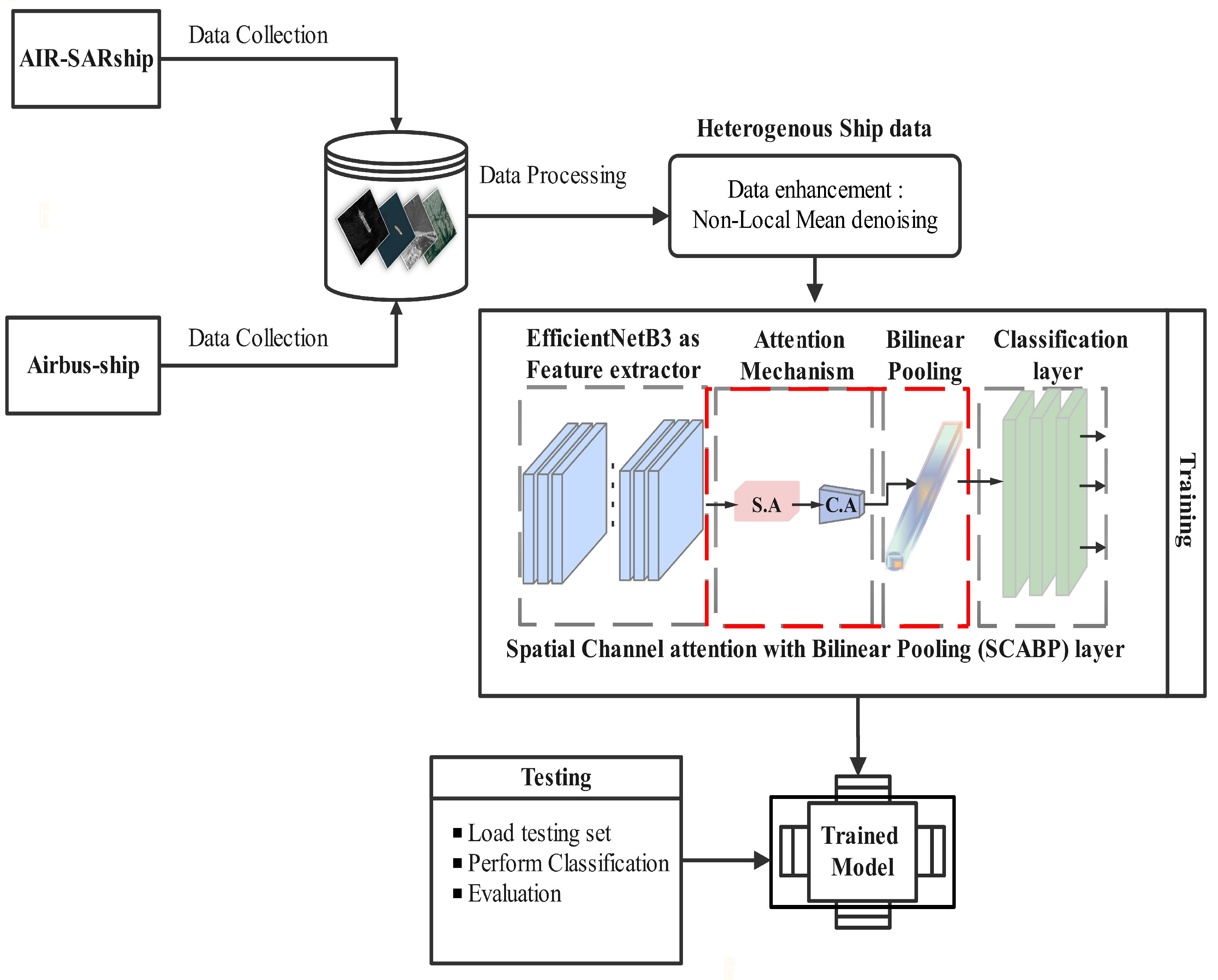Despite these advancements, the classification and detection of ships remain a challenging task due to various factors, including the spatial arrangement of geospatial objects, complex backgrounds, and the resolution limitations of sensor platforms [7,8]. Additionally, existing works rely on homogeneous datasets, either SAR or optical, which limits diversity. In light of these challenges, there is an imperative need for innovative solutions that can harness diverse data modalities and offer robustness against the complexities of maritime backgrounds. To address these challenges, this paper introduces a novel dataset termed Heterogeneous Ship data and a new technique called the Spatial–Channel Attention with Bilinear Pooling Network (SCABPNet).

The term “heterogeneous” refers to the combination of SAR and optical satellite imagery within a single dataset. This novel dataset amalgamates SAR and optical satellite imagery to harness a broader range of data modalities, enhancing the richness and diversity of information available for ship classification. The motivations behind the introduction of Heterogeneous Ship data can be summarized as follows. Firstly, by combining SAR and optical data, our approach overcomes the limitations of solely relying on a single data type. SAR images excel in capturing a larger area of the surroundings, regardless of time, weather conditions, or altitude [9,10]. On the other hand, optical images provide rich color and texture information. By merging these two data sources, we created a universal dataset that encompasses varying acquisition scenarios, making ship classification models more robust for real-time scenarios.

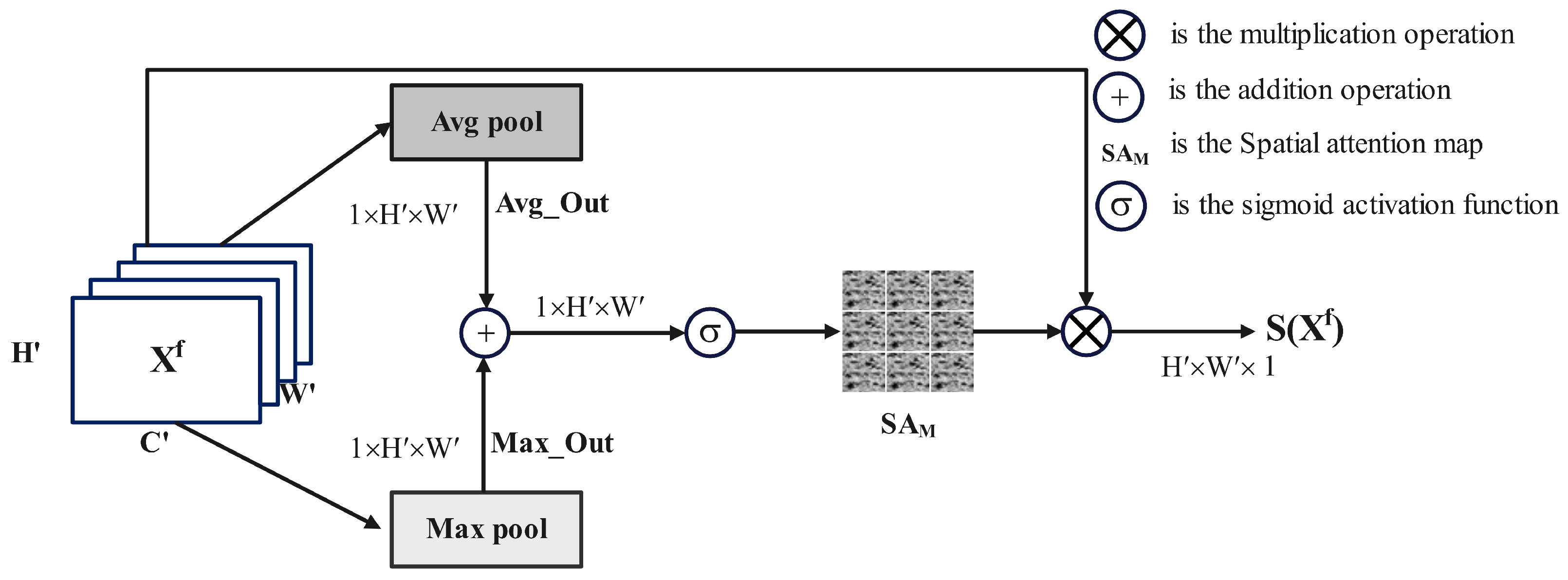
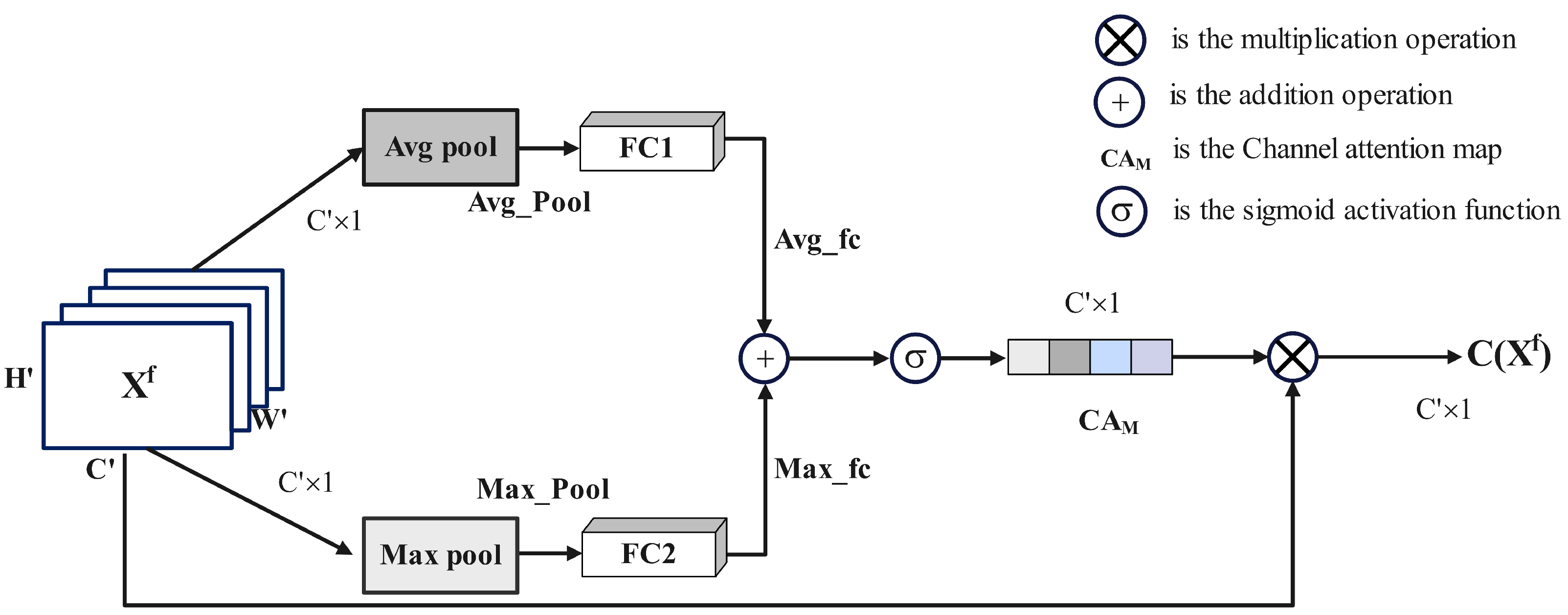
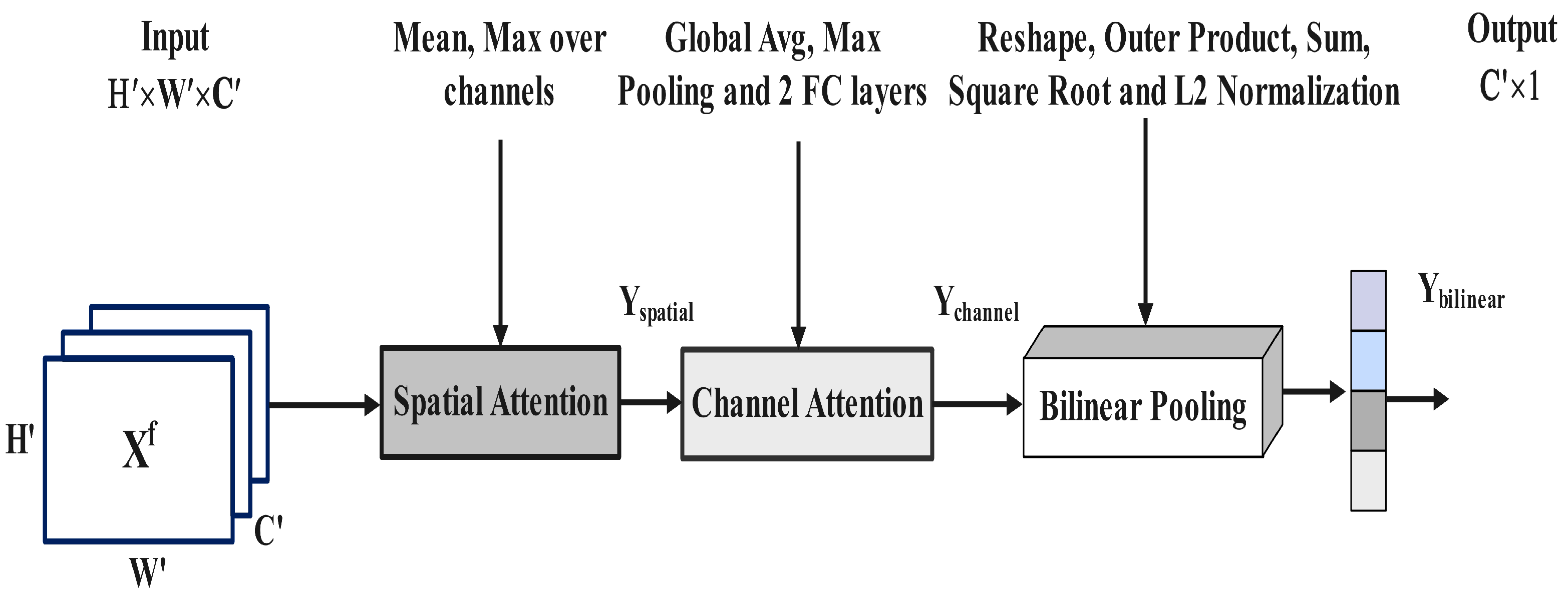
Additionally, motivated by the idea of overcoming the challenge of complex backgrounds in ship image datasets, we also propose an attention-based bilinear pooling approach called the Spatial–Channel Attention with Bilinear Pooling Network (SCABPNet). This approach combines spatial and channelwise information to effectively distinguish ships from the complex background, thereby enhancing the model’s classification performance. The use of Heterogeneous Ship data and the introduction of the SCABPNet approach offer several advantages. Firstly, the combination of SAR and optical satellite imagery provides a more-comprehensive representation of ships, incorporating complementary information from different modalities [11]. This fusion of data enhances the model’s ability to capture diverse ship characteristics, resulting in improved classification accuracy. Secondly, the SCABPNet approach addresses the challenge of complex backgrounds in target classification and detection. SCABPNet is able to effectively distinguish ships from sea clutter, coastlines, and other irrelevant background elements. By incorporating the spatial and channel attention mechanisms into a pooling technique, the SCABPNet approach is capable of focusing on salient ship-specific features while suppressing background noise and feature redundancy, leading to more-accurate ship classification results. Finally, the SCABPNet approach addresses the limitations of traditional ship monitoring techniques such as AIS and CFAR. In contrast, by incorporating these attention mechanisms and pooling techniques, SCABPNet maximizes the discriminative power of the Heterogeneous Ship data, resulting in enhanced classification performance. This represents a key advantage of our approach over conventional CNN models. The main contributions of our research are as follows:

• Heterogeneous Ship dataset: We present a novel dataset that combines SAR and optical satellite imagery, offering a richer and more-diverse set of features for ship classification, addressing the limitations of existing homogeneous datasets.
• SCABPNet model: A novel model that perfectly integrates spatial–channel attention with bilinear pooling, ensuring effective learning of discriminative specific ship features for classification tasks. Detailed ablation studies further elucidated the efficacy of the model.
• Comprehensive analysis: We conducted exhaustive experiments using the proposed SCABPNet model on the Heterogeneous Ship data, and on the MSTAR dataset, as well, then we compared their performance against existing state-of-the-art models, thereby establishing the superiority of the SCABPNet model.

Through this research, we aimed to provide a holistic solution to the challenges of ship image classification in remote sensing, thereby contributing to the advancement of this important field. The rest of this paper is arranged as follows: Section 2 reviews related work. Section 3 introduces the proposed Heterogeneous Ship data. Section 4 details the methodology, including the different components of SCABPNet. Section 5 presents the experiments conducted and discusses their results (the potential implications of our research in real-world scenarios). Finally, Section 6 concludes the paper and suggests potential research topics for future research.

2. Related Work

Ship image classification has seen significant advancements in recent years, with researchers exploring various approaches to improve classification accuracy. These approaches can be broadly categorized into three areas: using both Synthetic Aperture Radar (SAR) and optical datasets, incorporating attention mechanisms, and integrating improved pooling techniques.

Integration of SAR and optical datasets: The motivation behind integrating SAR and optical datasets is rooted in their complementary nature. For instance, SAR images excel in capturing the structural details of ships, while optical images provide rich color and texture information. In [12], Kanjir et al. surveyed the fusion of SAR and optical data, showcasing several studies that have capitalized on this integration over the past decade. A notable development in this field is the unified algorithm for vessel detection by Jubelin and Khenchaf (2014), which functions effectively across both SAR and optical imagery. They reported that a single detection algorithm can streamline the development and operational processes, a perspective contrasted by the findings in Kanjir et al.’s survey. This survey discusses the fact that dedicated algorithms, tailored to the unique attributes of each sensor type, might deliver superior results. Our research with the SCABPNet model contributes to this discourse by presenting a novel approach that aims to leverage the strengths of both modalities within a unified framework. This model challenges the view presented by Kanjir et al., demonstrating that a well-designed integrated system can indeed effectively bridge the diverse outputs of SAR and optical sensors, thereby enhancing ship detection and classification performance. Additionally, Rostami et al. [13] proposed a few-shot learning approach that utilizes cross-domain knowledge transfer from the optical dataset, designated as the source domain, to address a task in the SAR domain, identified as the target domain. Furthermore, other studies made use of both modalities (SAR and optical imageries) for classification tasks. Expanding beyond maritime applications, SAR–optical data have been used for classification in other domains like land cover, agriculture, etc. The studies by Shakya et al. [14] and Sreedhar et al. [15] demonstrated the broader utility of SAR-optical data fusion in areas like land cover and agriculture. Shakya et al. emphasized gradient-based data fusion for classification, while Sreedhar et al. highlighted the combined use of SAR’s all-weather imaging and the multispectral capabilities of optical datasets for time series analysis in crop classification. Further contributions in this evolving field include Prabhakar et al.’s method to refine noisy ground truth labels in SAR and optical image fusion in [16] and He et al.’s development of an oriented ship detector for remote sensing imagery in [17], underscoring the continuous innovation and application of these integrated techniques.

Advent of attention mechanisms: Attention mechanisms have emerged as powerful tools in ship image classification. These mechanisms enable models to selectively focus on relevant target-specific features while suppressing background noise [18]. They capture spatial and channelwise dependencies, allowing the model to attend to the most-discriminative regions and features. Several studies have explored attention-based approaches for ship image classification. For instance, Cui et al. [10] proposed a novel image-based convolutional network with Spatial Pyramid Aggregated Pooling (SPAP) and an attention mechanism called MAP-Net, which can learn features that are invariant, distinguishable, repeatable, and suitable for cross-modal image matching. They evaluated their method on five sets of multisource and multiresolution SAR and optical images and demonstrated that it achieved superior performance compared to the state-of-the-art methods. Additionally, Zhao et al. [19] proposed a spatial attention mechanism to highlight informative regions in ship images, while Hu et al. [20] introduced a channel attention mechanism to emphasize relevant features. Both studies showed promising results in improving ship classification accuracy by effectively capturing fine-grained details and enhancing the model’s discriminative capacity. Further, Sun et al. [21] implemented a Strong-Scattering-Point-Aware Network (SPAN), which recognizes ship categories based on the distribution characteristics of strong scattering points. Their approach underscores the potential of attention mechanisms in ship detection and classification in SAR images. In [22], another study conducted by Zhao et al. highlighted a multitask learning framework for object recognition and detection in SAR images, emphasizing the potential of attention mechanism techniques in recognizing small, weak, and dense targets in SAR images.

Improved pooling techniques: Bilinear techniques have gained attention in ship image classification and detection due to their ability to capture complex interactions between spatial and channelwise information. Bilinear pooling, in particular, enables the modeling of complex relationships within the input data through elementwise multiplications between spatial and channelwise features, followed by summation. This technique has proven effective in ship-image-classification tasks. For example, Li et al. [23] introduced an improved bilinear pooling technique to construct a compact bilinear CNN model. They specifically incorporated a joint pooling approach to diminish the dimensionality of bilinear features, facilitating their integration into a bilinear CNN framework for end-to-end optimization. Furthermore, He et al. [24] developed a novel Group Bilinear Convolutional Neural Network (GBCNN) model to extract discriminative second-order representations of ship targets from the pairwise Vertical–Horizontal polarization (VH) and Vertical–Vertical polarization (VV) SAR images, yielding state-of-the-art performance. Similarly, Lin et al. [25,26,27] applied bilinear pooling in ship classification and demonstrated its ability to capture rich interactions and enhance discriminative power. Additionally, Li et al. [28] introduced a Multimodal Bilinear Fusion Network (MBFNet) for hyperspectral and SAR image classification, achieving effective land cover classification performance. These studies highlight the effectiveness of bilinear techniques in image classification.

Despite these advancements, there are still challenges in ship image classification that need to be addressed. These include the need for more-effective integration of SAR and optical datasets, more-sophisticated attention mechanisms, and more-powerful bilinear techniques. Motivated by these underlying challenges and inspired by previous academic endeavors, we propose the SCABPNet model, which combines these techniques to further enhance classification performance.

3. Proposed Heterogeneous Ship Data

Remote sensing constantly suffers from the inherent complexity of dealing with diverse datasets. In the context of ship image classification, this complexity is greatly amplified when addressing the challenges posed by Heterogeneous Ship data. This proposed dataset aimed to serve as a robust, diverse platform that encapsulates the complexities and distinct features of real-world scenarios. However, the richness and diversity of the dataset also introduce multiple challenges that require further investigation.

Variability of ship types: Our dataset encompasses a range of ship types—from transport vessels to oil tankers and fishing boats. Each of these ship categories presents its own set of features and structural complexities, rendering the classification task more challenging than initially perceived. The distinctiveness of these ships in terms of size, structural design, and functionalities inevitably introduces a high degree of intra-class variability [29,30].

Geographical and environmental differences: The images in our dataset were sourced from diverse geographical regions, each with its own set of challenges. The variations in coastlines, water turbidity, lighting conditions, and even man-made buildings can drastically alter the appearance of ships in the imagery [31]. Further, changes in weather conditions, sea state, and seasonal effects may introduce inconsistencies across images, complicating the classification task [3].

Interference and clutter: The inclusion of both offshore and, notably, inshore ship images introduces the substantial challenge of land interference. Ships near the coast might be obscured by coastal infrastructure or their features might blend with reflections from adjacent terrains, making them harder to distinguish [32].

Heterogeneity of sensor data: With SAR data sourced from satellites like Gaofen-3 and Sentinel-1 [33] and optical images from the Airbus Ship Detection dataset [34,35], there is a sharp difference in the imaging mechanisms. These satellites capture imagery at different resolutions, frequencies, and imaging modes. While SAR provides all-weather, day-and-night imaging capabilities, it may also introduce speckle noise. Conversely, optical images, although rich in color information, can be obscured by cloud cover and varying lighting conditions [36,37].

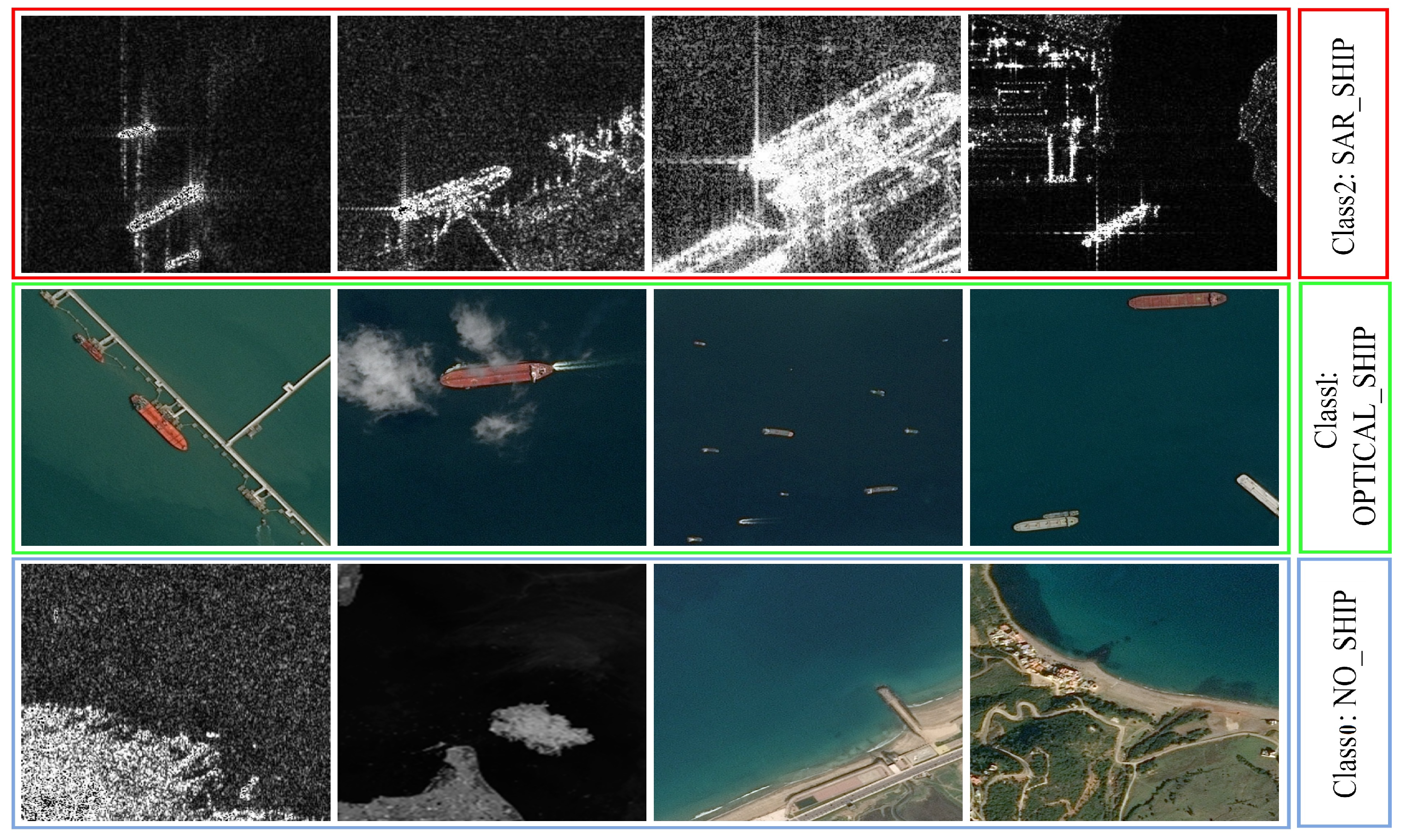
To sum up, the proposed dataset is made up of three classes: no ship (Class 0), optical ship (Class 1), and SAR ship (Class 2). It contains 4962 images, with 20% set aside for validation and the rest for training.

Table 1. Heterogeneous Ship dataset splitting details.

Class	Training Set	Testing Set	Total
SAR ship	1654	330	1984
Optical ship	1654	330	1984
No ship	1654	330	1984
TOTAL	4962	990	5952

shows the partition of the dataset, with a balanced distribution of images across the three categories. Figure 1 provides a visualization of the proposed Heterogeneous Ship data, with different colors representing different classes.

To address the above challenges and improve the quality of the images, we applied image pre-processing and denoising techniques. The denoising technique used in this research was the Non-Local Means Algorithm. Despite its proven efficacy, it has limits and cannot solve every problem. While it reduces noise, ensuring the preservation of important ship features in the imagery remains a challenge. Furthermore, the inherent noise characteristics of SAR (speckle) differ from those in optical images, necessitating a fine-tuning setting of the Non-Local Means Algorithm for each modality. This algorithm was chosen due to its effectiveness in image processing, particularly in reducing noise while preserving important image details. The Non-Local Means Algorithm corrects the value of the center pixel in an image by moving a ‘search window’ over the image and averaging the values in the window [38]. The Non-Local Means Algorithm used during the experiment is described in Algorithm 1. The mathematical representation of this technique is as follows:

Given a noisy image v = {$v\left(i\right)$|i∈I}, we can compute the estimated pixel values as follows:

$$NL\left[v\right]\left(i\right)=\sum _{j\in I}w(i,j)v\left(j\right)$$

(1)

where I is the image domain, i and j are the pixel values in the noisy image, $w(i,j)$ is the similarity between the pixels i, and j (0 ≤ $w(i,j)$ ≤ 1). Also, $w(i,j)$ is computed as follows:

$$w(i,j)=\frac{1}{z\left(i\right)}ex{p}^{-\frac{d(i,j)}{h^2}}$$

(2)

$$d(i,j)=\parallel v\left(N_i\right)-v\left(N_j\right){\parallel }_{2,\alpha }^2$$

(3)

where $z\left(i\right)$ is a normalization factor, $\alpha$ is the standard deviation, h is the smoothing parameter, and $d(i,j)$ is the Euclidean distance between the pixel intensities of the local neighborhood. The Non-Local Means Algorithm used during the experiment is as follows.

Algorithm 1 Non-Local Means Algorithm.

1:     $\mathbf{Step}\mathbf{1}:\mathrm{Load}\mathrm{input}\mathrm{images}.$   2:     $\mathbf{Step}\mathbf{2}:\mathrm{Use}\mathrm{Equation}\left(2\right)\mathrm{to}\mathrm{compute}\mathrm{the}\mathrm{similarity}$   3:      $\mathrm{between}\mathrm{pixels}i\mathrm{and}j.$   4:     $\mathbf{Step}\mathbf{3}:\mathrm{Define}\mathrm{a}\mathrm{search}\mathrm{window},\mathrm{and}\mathrm{use}\mathrm{Equation}\left(2\right)$   5:      $\mathrm{to}\mathrm{compute}\mathrm{the}\mathrm{similarity}\mathrm{of}\mathrm{search}\mathrm{window}.$   6:     $\mathbf{Step}\mathbf{4}:\mathrm{Compute}\mathrm{the}\mathrm{estimated}\mathrm{pixels}\mathrm{values}\mathrm{by}$   7:      $\mathrm{applying}\mathrm{Equation}\left(1\right)\mathrm{for}\mathrm{image}\mathrm{denoising}.$   8:     $\mathbf{Step}\mathbf{5}:\mathrm{Generate}\mathrm{new}\mathrm{images}\mathrm{free}\mathrm{of}\mathrm{noise}.$

The current Heterogeneous Ship data were substantially updated in this study. Originally comprising a total of 4630 images, the dataset was expanded to a total of 5952 images. This expansion enhanced the dataset’s robustness, allowing for more-comprehensive training and evaluation of our SCABPNet model. Moreover, the updated dataset featured a revised class configuration in the no ship category, now comprising an equal ratio of 50% SAR images and 50% optical images. Furthermore, we used Augmentor, a Python package for data augmentation, to balance the number of images in each class. These updates to the Heterogeneous Ship data represent a significant enhancement over our previous dataset. In summary, the combination of SAR and optical satellite imagery provides a more-comprehensive representation of ships, incorporating complementary information from different modalities.

4. Proposed Framework: Spatial–Channel Attention with Bilinear Pooling Network

The proposed framework was composed of two major components: EfficientNetB3 as a backbone model and a custom attention-based layer (SCABP). In this study, EfficientNetB3 was utilized as the base model for feature extraction due to its proven effectiveness in handling complex image data. The main objective of the proposed solution was the implementation of a custom layer, the Spatial–Channel Attention with Bilinear Pooling (SCABP) layer. This layer employs both spatial and channel attention mechanisms to highlight important features in the input and, then, uses bilinear pooling to create a richer representation of these features. The proposed model, as depicted in Figure 2, was designed to effectively handle the complexities of ship data. The SCABP layer, highlighted in the red box, is a key component of our model.

4.1. Attention Mechanism Approach

The attention mechanism used in this work is known as the dual-attention mechanism. Our dual-attention mechanism employs sequentially both spatial and channel attention mechanisms, enabling the model to focus on salient regions within each feature map (spatial attention) and the most-informative feature maps (channel attention). In Figure 3 and Figure 4, the architecture of our dual-attention is displayed.

The spatial attention mechanism in this article differs from the traditional spatial attention mechanism in some ways:

• Original spatial attention mechanism: In a typical spatial attention mechanism, an attention map that highlights the spatial areas of the input is created. This is often performed by using a convolutional layer (or multiple layers) to process the input feature maps and output a single feature map of the same width and height, but with a single channel. This output feature map can be viewed as a “mask” that emphasizes the important regions and suppresses the less-important ones [39,40]. The main steps involved in a typical spatial attention mechanism are as follows: Apply a convolutional layer to the input feature maps to create a combined feature map. Apply a sigmoid function to the combined feature map to generate the attention map.
• Our spatial attention mechanism approach: The spatial attention mechanism we introduce is simpler and slightly different. It calculates the average and maximum along the channel axis of the input feature maps separately, resulting in two different spatial attention maps. These two maps are then added together. A sigmoid function is applied to the result to generate the final spatial attention map. To sum up, for a given input tensor X with dimensions $(H,W,C)$ (height, width, channels), the extracted feature map is defined as $X^f$ with dimensions $(H^{\prime },W^{\prime },C^{\prime })$ (height, width, channels), the mean and maximum across the channel dimension were computed, and a sigmoid activation function was applied to the resulting output using the equations below.

  $$\mathrm{Avg}\_\mathrm{Out}=\frac{1}{C^{\prime }}\sum _{k=1}^{C^{\prime }}{X}_{ijk}^f\mathrm{Avg}\_\mathrm{Out}\in {\mathbb{R}}^{H^{\prime }\times W^{\prime }}$$

  (4)

  $$\mathrm{Max}\_\mathrm{Out}=\underset{k=1}{\overset{C^{\prime }}{\max }}{X}_{ijk}^f\mathrm{Max}\_\mathrm{Out}\in {\mathbb{R}}^{H^{\prime }\times W^{\prime }}$$

  (5)
  Here, $X_{ijk}^f$ is the feature value at spatial location (i,j) in the channel k. Additionally, i∈$[1,H^{\prime }]$, j∈$[1,W^{\prime }]$, and k∈$[1,C^{\prime }]$ are the indices for the height, width, and channel dimensions, respectively. The operations $\frac{1}{C^{\prime }}{\sum }_{k=1}^{C^{\prime }}{X}_{ijk}^f$ and ${\max }_{k=1}^{C^{\prime }}{X}_{ijk}^f$ compute the average and maximum over the channel dimension, resulting in a two-dimensional matrix ($\mathrm{Avg}\_\mathrm{Out}$ and $\mathrm{Max}\_\mathrm{Out}$) of the same size: $H^{\prime }\times W^{\prime }$. The output $S\left(X^f\right)$ of the spatial attention can be obtained as

  $$S\left(X^f\right)=\sigma \left(\frac{1}{C^{\prime }}\sum _{k=1}^{C^{\prime }}{X}^f[:,:,k]+\underset{k\in [1,C^{\prime }]}{\max }{X}^f[:,:,k]\right),S\left(X^f\right)\in {\mathbb{R}}^{H^{\prime }\times W^{\prime }\times 1}$$

  (6)
  In this study, we used a spatial attention mechanism that differs from the original one in two main ways. First, instead of using a trainable convolutional layer, we used fixed operations to extract the attention map, making it entirely data-driven. Second, our approach utilizes both average and maximum values, while typical spatial attention mechanisms use only one or the other. By combining both, we were able to capture more diverse spatial information.

The channel attention mechanism in this study and the original channel attention mechanism proposed in the Squeeze-and-Excitation (SE) Network [20] have similar goals, but differ in a few ways:

• The original channel attention mechanism in the SE Network involves the following steps: Global average pooling is applied to the feature maps to capture the global spatial information. The pooled features are passed through two Fully Connected (FC) layers (the “Squeeze” and “Excitation” operations). The first FC layer reduces the dimensions of the features by a reduction ratio (this is the “Squeeze” operation), and the second FC layer restores the dimensions back to the original number of channels (this is the “Excitation” operation). The output of the second FC layer is a set of channelwise weights, which are used to reweight the original feature maps.
• In comparison, our proposed channel attention mechanism has the following differences: both global average pooling and global max pooling are used, and their results are processed separately using the equations below:

  $$\mathrm{Avg}\_\mathrm{Pool}=\frac{1}{H^{\prime }\times W^{\prime }}\sum _{i=1}^{H^{\prime }}\sum _{j=1}^{W^{\prime }}{X}^f[i,j,:],\mathrm{Avg}\_\mathrm{Pool}\in {\mathbb{R}}^{C^{\prime }\times 1}$$

  (7)

  $$\mathrm{Max}\_\mathrm{Pool}=\underset{i\in [1,H^{\prime }],j\in [1,W^{\prime }]}{\max }{X}^f[i,j,:],\mathrm{Max}\_\mathrm{Pool}\in {\mathbb{R}}^{C^{\prime }\times 1}$$

  (8)
  Furthermore, both outputs are passed through two Fully Connected layers (FC1 and FC2).

  $$\mathrm{Avg}\_\mathrm{fc}=\mathrm{FC}1(\mathrm{Avg}\_\mathrm{Pool})$$

  (9)

  $$\mathrm{Max}\_\mathrm{fc}=\mathrm{FC}2(\mathrm{Max}\_\mathrm{Pool})$$

  (10)
  Avg_fc and Max_fc are two vectors of size $N1$ and $N2$. $N1$ is the number of neurons of the Fully Connected layer FC1, and $N2$ is the number of neurons of the Fully Connected layer FC2. The two vectors are added together before being passed through the sigmoid activation function to obtain the channel attention weights ($C\left(X^f\right)$) by applying the equation below:

  $$C\left(X^f\right)=\sigma (\mathrm{Avg}\_\mathrm{fc}+\mathrm{Max}\_\mathrm{fc}),C\left(X^f\right)\in {\mathbb{R}}^{C^{\prime }\times 1}$$

  (11)
  This is a form of “feature fusion”, which is not present in the original SE Network. The channel attention weights are used to multiply the original features directly in the channel dimension without a “rescaling” step present in the SE Network. These modifications in the SCABP layer were designed to enhance the channel attention mechanism, potentially making it more capable of capturing important features and improving the model’s performance.

4.2. Bilinear Approach

The bilinear pooling operation is a technique that calculates the outer products of features. This helps in capturing second-order feature interactions that traditional pooling methods such as max pooling or average pooling are unable to capture. The bilinear pooling operation aims to provide a more-detailed representation of the input, giving a richer and more-nuanced insight into the data. In this specific experiment, the bilinear pooling operation was used to capture second-order feature interactions between channels, which aimed to provide more-detailed and comprehensive representations of the data. This can ultimately enhance model performance for specific tasks:

• Original bilinear pooling: The input tensor is reshaped into a 2D matrix, and the outer product of this matrix with itself is computed to capture second-order feature interactions. The signed square root is applied to the resulting tensor to introduce non-linearity and manage high dimensionality. Finally, $l2$ normalization is performed to ensure that the scale of the features does not overly influence the learning process [14,25].
• Our bilinear pooling approach: The initial steps are the same: $X_{\mathrm{reshaped}}^f$ is computed by applying a reshape operation to the input tensor as follows:

  $$X_{\mathrm{reshaped}}^f=\mathrm{reshape}(X^f,(\mathrm{batch}\_\mathrm{size},H^{\prime }\times W^{\prime },C^{\prime }))$$

  (12)

  where $X_{\mathrm{reshaped}}^f\in {\mathbb{R}}^{\mathrm{batch}\_\mathrm{size}\times H^{\prime }\times W^{\prime }\times C^{\prime }}$ is a 4D tensor. The reshape operation converts this 4D tensor into a 3D tensor with dimensions: batch_size × $\left(H^{\prime }{W}^{\prime }\right)$ × $C^{\prime }$. This reshaping operation simply rearranges the values within the tensor and changes its dimensionality without changing the total number of values in the tensor.
  Moreover, the outer product (outer_product) can be obtained as

  $$\mathrm{outer}\_\mathrm{product}={\left(X_{\mathrm{reshaped}}^f\right)}^T{X}_{\mathrm{reshaped}}^f$$

  (13)

  where $\mathrm{outer}\_\mathrm{product}\in {\mathbb{R}}^{\mathrm{batch}\_\mathrm{size}\times (H^{\prime }\times W^{\prime })\times (H^{\prime }\times W^{\prime })}$. Equation (13) calculates the outer product of the reshaped tensor with itself. The outer product is a generalization of the vector outer product to the tensors. For a given tensor, the result of this operation is a tensor of a rank that is the sum of the ranks of the operands. The superscript “T” denotes the transpose of the tensor. Here, the transpose operation is applied to the last two dimensions of $X_{\mathrm{reshaped}}^f$, which is a common approach when working with batches of data. Furthermore, the sum of the outer product (sum_outer_product) can be obtained as

  $$\mathrm{sum}\_\mathrm{outer}\_\mathrm{product}=\sum _{i=1}^{H^{\prime }\times W^{\prime }}\sum _{j=1}^{H^{\prime }\times W^{\prime }}\mathrm{outer}\_\mathrm{product}(i,j)$$

  (14)

  where $\mathrm{sum}\_\mathrm{outer}\_\mathrm{product}\in {\mathbb{R}}^{\mathrm{batch}\_\mathrm{size}\times C^{\prime }\times C^{\prime }}$ is the tensor dimension. Conceptually, this sum operation aggregates all the bilinear interactions obtained from the outer product across all spatial positions. Note that, in our bilinear approach, while computing the sum_outer_product_sqrt, instead of using a signed square root operation, the square root of the absolute approach is used, and a small constant $\epsilon ={10}^{-7}$ is added for numerical stability by applying this equation:

  $$\mathrm{sum}\_\mathrm{outer}\_\mathrm{product}\_\mathrm{sqrt}=\sqrt{|\mathrm{sum}\_\mathrm{outer}\_\mathrm{product}|+\epsilon }$$

  (15)

  where $\mathrm{sum}\_\mathrm{outer}\_\mathrm{product}\_\mathrm{sqrt}\in {\mathbb{R}}^{\mathrm{batch}\_\mathrm{size}\times C^{\prime }}$. This step introduces non-linearity and manages high dimensionality, but does not distinguish between positive and negative values as the signed square root does. Finally, $l2$ normalization is performed. Normalization ensures that the values are within a certain range, in our case (0,1). This is often performed to ensure numerical stability, as well as to put different features on the same scale. The notation ${|·|}_2$ represents the L2 norm, or Euclidean norm, which is a measure of the length of a vector. In summary, the primary difference between the two lies in the non-linearity step and taking the square root of the absolute value to ensure it is non-negative. Finally, the bilinear output $B\left(X^f\right)$ can be expressed as

  $$B\left(X^f\right)=\frac{\mathrm{sum}\_\mathrm{outer}\_\mathrm{product}\_\mathrm{sqrt}}{{|\mathrm{sum}\_\mathrm{outer}\_\mathrm{product}\_\mathrm{sqrt}|}_2}$$

  (16)

  where $B\left(X^f\right)\in {\mathbb{R}}^{\mathrm{batch}\_\mathrm{size}\times C^{\prime }}$.

4.3. SCABP Layer

Our proposed model’s core is the SCABP layer. It applies spatial attention, channel attention, and bilinear pooling sequentially to the input, as shown in Figure 5. The SCABP layer transforms the input through Equations (17)–(19). The steps summarizing the transformations occurring within our SCABPNet are described in Algorithm 2.

$$Y_{\mathrm{spatial}}=X^f\odot S\left(X^f\right),Y_{\mathrm{spatial}}\in {\mathbb{R}}^{H^{\prime }\times W^{\prime }\times 1}$$

(17)

$$Y_{\mathrm{channel}}=\mathrm{reshape}\left(Y_{\mathrm{spatial}}\right)\odot C\left(\mathrm{reshape}\left(Y_{\mathrm{spatial}}\right)\right),Y_{\mathrm{channel}}\in {\mathbb{R}}^{C^{\prime }\times 1}$$

(18)

$$Y_{\mathrm{bilinear}}=B\left(Y_{\mathrm{channel}}\right),Y_{\mathrm{bilinear}}\in {\mathbb{R}}^{C^{\prime }\times 1}$$

(19)

where $X^f$ is the given input tensor, $Y_{\mathrm{spatial}}$ is the output of the spatial attention, $Y_{\mathrm{channel}}$ is the output of the channel attention, and $Y_{\mathrm{bilinear}}$ is the final output of the SCABP layer.

Algorithm 2 The proposed SCABPNet algorithm.

1: Input: Image $X\in {\mathbb{R}}^{H\times W\times C}$    2: Output: Class prediction $\widehat{y}$    3: Feature extraction using base model (EfficientNetB3)    4: $X^f=f_{\mathrm{EfficientNetB}3}\left(X\right)\in {\mathbb{R}}^{H^{\prime }\times W^{\prime }\times C^{\prime }}$    5: Apply SCABP layer    6:    Spatial attention:    7: Use (6) to compute $S\left(X^f\right)$ with $S\left(X^f\right)$$\in {\mathbb{R}}^{H^{\prime }\times W^{\prime }\times 1}$    8: $Y_{\mathrm{spatial}}=X^f\odot S\left(X^f\right)$    9:     Channel attention:  10: Use (7) and (8) to compute Avg_Pool and Max_Pool with Avg_Pool and Max_Pool $\in {\mathbb{R}}^{C^{\prime }\times 1}$  11: Use (9) and (10) to compute Avg_fc and Max_fc with Avg_fc and Max_fc $\in {\mathbb{R}}^{\frac{C^{\prime }}{r}\times 1}$  12: Use (11) to compute $C\left(X^f\right)$ with $C\left(X^f\right)$$\in {\mathbb{R}}^{C^{\prime }\times 1}$  13: $Y_{\mathrm{channel}}=\mathrm{reshape}\left(Y_{\mathrm{spatial}}\right)\odot C\left(\mathrm{reshape}\left(Y_{\mathrm{spatial}}\right)\right)$  14:     Bilinear pooling:  15: Use (16) to compute $B\left(X^f\right)$$\in {\mathbb{R}}^{\mathrm{batch}\_\mathrm{size}\times C^{\prime }}$  16: $Y_{\mathrm{bilinear}}=B\left(Y_{\mathrm{channel}}\right)$  17: Classification layers : $\widehat{y}=\mathrm{Softmax}\left(\mathrm{FC}5\left(\mathrm{FC}4\left(\mathrm{FC}3\left(\mathrm{FC}2\left(\mathrm{FC}1\left(B\left(X^f\right)\right)\right)\right)\right)\right)\right)$

⊙ denotes elementwise multiplication; r stands for the reduction ratio; $\sigma$ is the sigmoid function; FC are Fully Connected layers.

Table 2. Summary of SCABPNet’s parameters.

Layer (Type)	Filter Size	Number of Parameters
InputLayer	224	0
SCABP	49	103,720
Dense (ReLU)	512	25,600
Dropout (0.55)	-	0
Dense (ReLU)	480	246,240
Dropout (0.25)	-	0
Dense (ReLU)	224	107,744
Dropout (0.55)	-	0
Dense (ReLU)	32	7200
Dense (ReLU)	32	1056
Dense (Softmax)	3	99

provides a comprehensive overview of the proposed model’s architecture, detailing the type, filter size, and number of parameters for each layer. This information is crucial for understanding the complexity and capacity of SCABPNet.

5. Experiments and Discussion

In this section, we provide an overview of the experiments conducted on the proposed model using the Heterogeneous Ship data. Additionally, we evaluated the effectiveness of SCABPNet by conducting the same experiments on the MSTAR dataset. We present the details of the experimental setup, the evaluation metrics, and the results. Furthermore, we conducted ablation studies to analyze the contributions of the SCABP layer. We also provide comparisons with the CBAM approach and conclude with a discussion.

5.1. Experimental Settings

Our SCABPNet model was implemented using the TensorFlow library, and the hyperparameters of the proposed method were meticulously optimized to enhance the classification performance. The SCABPNet model was configured with an input size of 224 × 224. The Adam optimizer was employed for training, with the epoch number and batch size set to 500 and 16, respectively. These values were determined based on preliminary experiments that demonstrated an optimal balance between computational efficiency and model performance. The initial learning rate was set to 0.001, and the exponential decay factor was statistically adjusted to match the learning rate’s equivalent value, with a clip value of 0.2. To mitigate overfitting, the dropout rate was set to the expected values of 0.55 and 0.25. The image data generator performed operations such as rescaling (1/255), rotation (range = 10), width shift (range = 0.2), height shift (range = 0.2), shear (range = 0.2), zoom (range = 0.2), and horizontal flip. The callback learning rate adjustment was set to ReduceLROnPlateau, with parameters including ‘Val loss’ monitoring, a factor of 0.1, an epsilon of ${10}^{-6}$, a patience of 10, a verbose of 1, and the mode set to ‘min’. A custom focal loss was utilized as the loss function during training.

Table 3. Hyperparameters of the training.

Type	Method	Value	Description
Structural and non-structural	Lr	0.001	Initial learning rate
	Epoch	500	Number of training epochs
	decay	0.2	Exponential decay factor
	Dropout	0.55 and 0.25	Randomly drop layers
	Batch size	16	Subsamples for training
Data augmentation	Rescale	1/255	Rescaling factor
	Rotation	30	Range of rotation
	Width shift	0.2	Range of width shift
	Height shift	0.2	Range of height shift
	Shear	0.2	Range of shear
	Horizontal flip	True	Flip images horizontally

summarizes the hyperparameters used in this experiment.

5.2. Evaluation Metrics

The experiment’s performance was quantitatively evaluated using metrics such as the classification report, confusion matrix, Receiver Operating Characteristics (ROCs), and the Area Under the Curve (AUC). Precision (Pre), Recall (Rec), F1-score (F1), Accuracy (Acc), and ROC/AUC were calculated using the following equations:

$$\mathrm{Precision}=\frac{\mathrm{TP}}{\mathrm{TP}+\mathrm{FP}}$$

(20)

$$\mathrm{Recall}=\frac{\mathrm{TP}}{\mathrm{TP}+\mathrm{FN}}$$

(21)

$$\mathrm{F}1-\mathrm{score}=2\times \frac{\mathrm{Precision}\times \mathrm{Recall}}{\mathrm{Precision}+\mathrm{Recall}}$$

(22)

$$\mathrm{Accuracy}=100\times \frac{\mathrm{TP}+\mathrm{TN}}{(\mathrm{TP}+\mathrm{TN})+(\mathrm{FP}+\mathrm{FN})}$$

(23)

$$\mathrm{FPR}=\frac{\mathrm{FP}}{\mathrm{FP}+\mathrm{TN}}$$

(24)

$$\mathrm{TPR}=\frac{\mathrm{TP}}{\mathrm{TP}+\mathrm{FN}}$$

(25)

$$\mathrm{ROC}\mathrm{Curve}\text{:}\left(\mathrm{FPR},\mathrm{TPR}\right)$$

(26)

The ROC curve is obtained by plotting the TPR vs. the FPR at different classification threshold settings.

$$\mathrm{AUC}={\int }_0^1\mathrm{ROC}\left(t\right)dt$$

(27)

The AUC provides an aggregate measure of model performance across all possible classification thresholds, where $TP$ denotes True Positive, $TN$ denotes True Negative, $FP$ denotes False Positive, $FN$ denotes False Negative, $FPR$ is the False Positive Rate, and $TPR$ is the True Positive Rate. Finally, t is the classification threshold.

5.3. Experimental Results of Proposed Solution and Baseline + CBAM

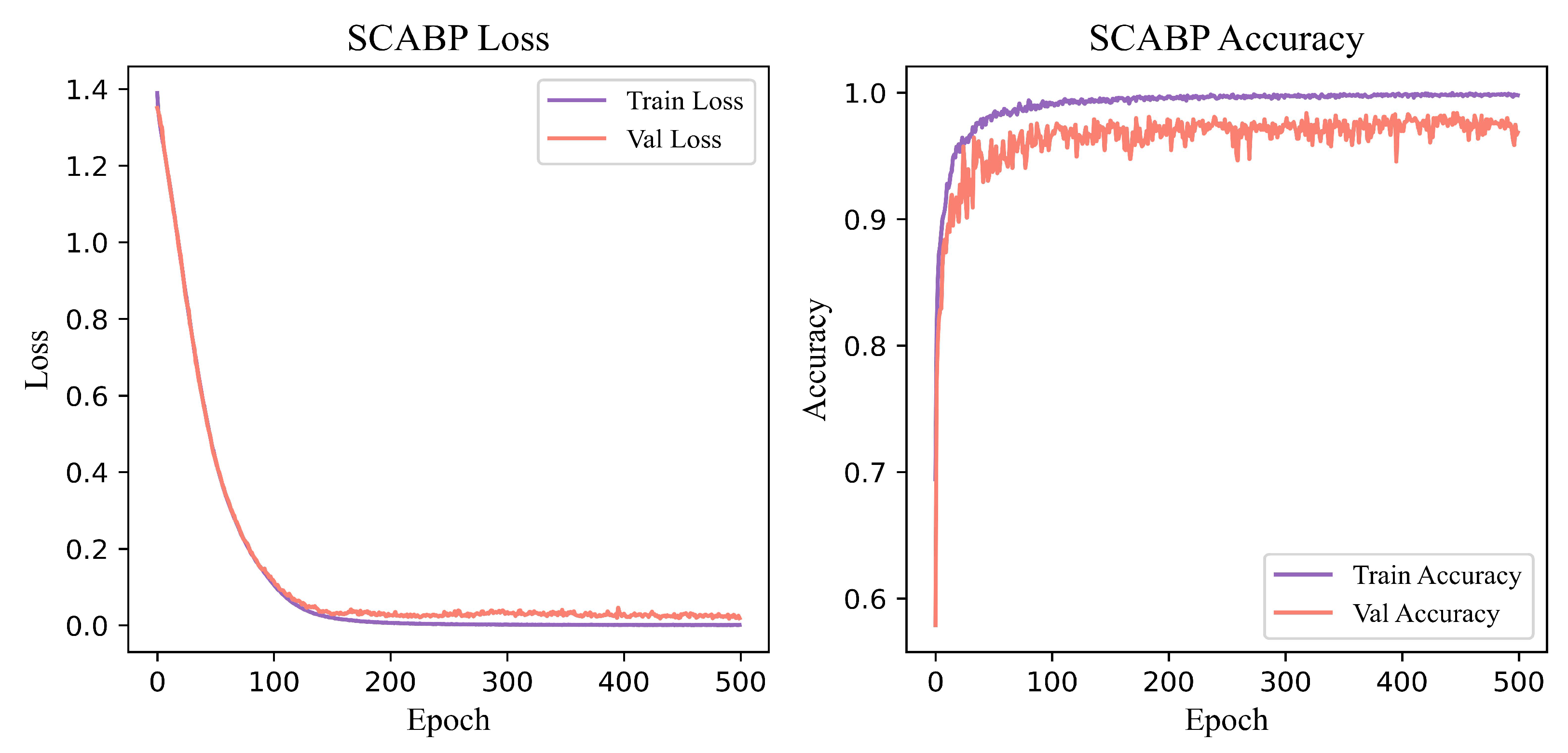
This section highlights the results of SCABPNet’s performance on the proposed Heterogeneous Ship data and the Baseline + CBAM model. First, our SCABPNet achieved an accuracy of 97.67%, a precision of 97.78%, a recall of 97.67%, and an F1-score of 97.68%, as indicated in

Table 4. Overall performance of SCABPNet model on the Heterogeneous Ship data.

	Precision	Recall	F1-Score	Support
SAR ship	1	0.9545	0.9767	330
Optical ship	0.9426	0.9969	0.9690	330
No ship	0.9907	0.9787	0.9847	330
Overall	0.97783	0.9767	0.9768	990
Accuracy			0.9767	990
Macro avg	0.9778	0.9767	0.9768	990
Weighted avg	0.9778	0.9767	0.9768	990

, on the testing set. In Figure 6, SCABPNet’s training curves show how the model converged during training. Second,the Baseline + CBAM model recorded an accuracy of 95.45%, a precision of 95.77%, a recall of 95.45%, and an F1-score of 95.46%, as indicated in

Table 5. Overall performance of Baseline + CBAM model on the Heterogeneous Ship data.

	Precision	Recall	F1-Score	Support
SAR ship	1	0.9000	0.9474	330
Optical ship	0.9033	0.9909	0.9451	330
No ship	0.9698	0.9727	0.9713	330
Overall	0.9577	0.9545	0.9546	990
Accuracy			0.9545	990
Macro avg	0.9577	0.9545	0.9546	990
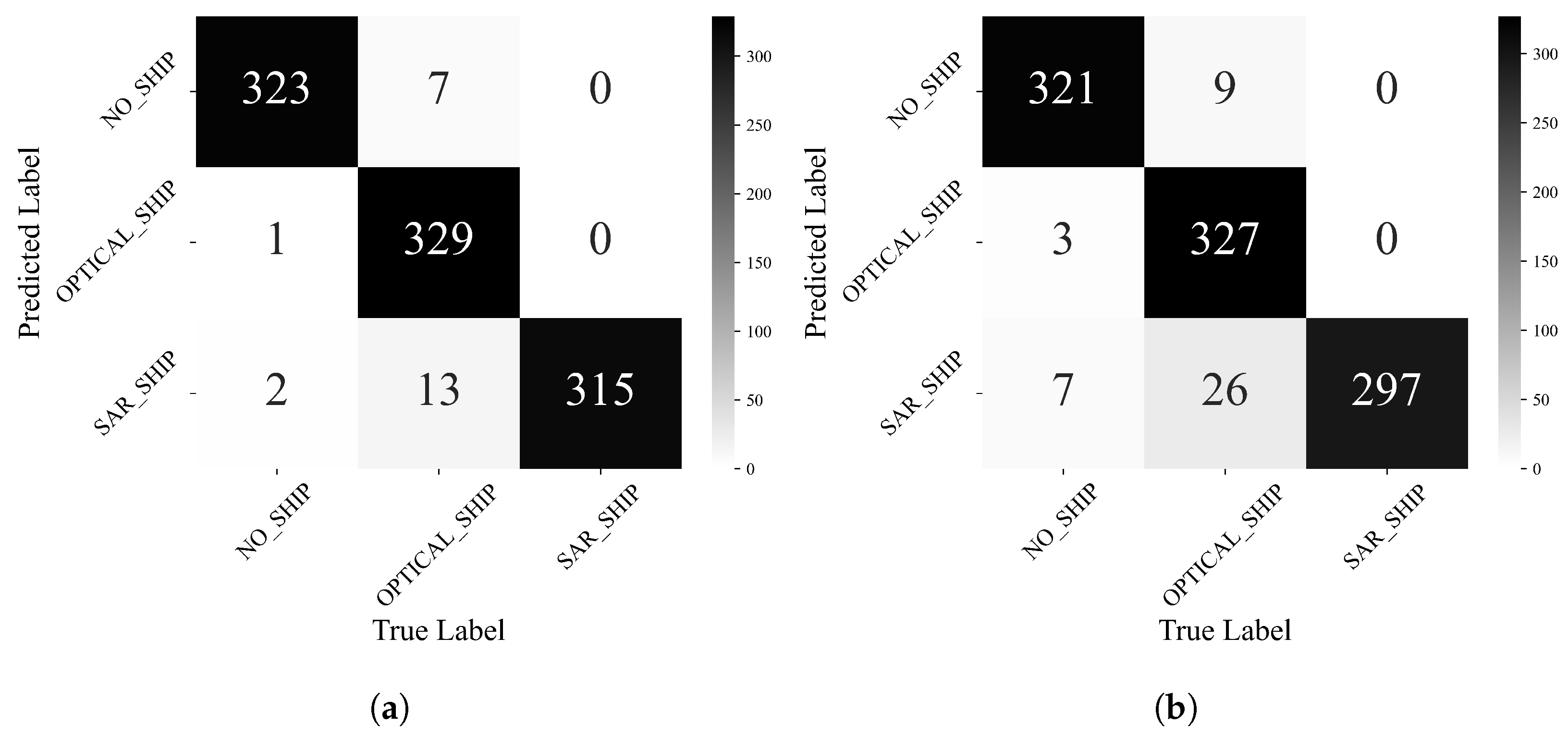
Weighted avg	0.9577	0.9545	0.9546	990

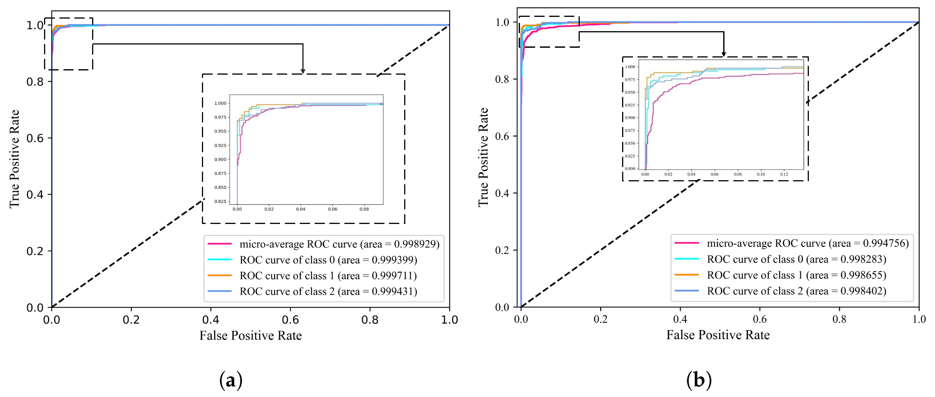
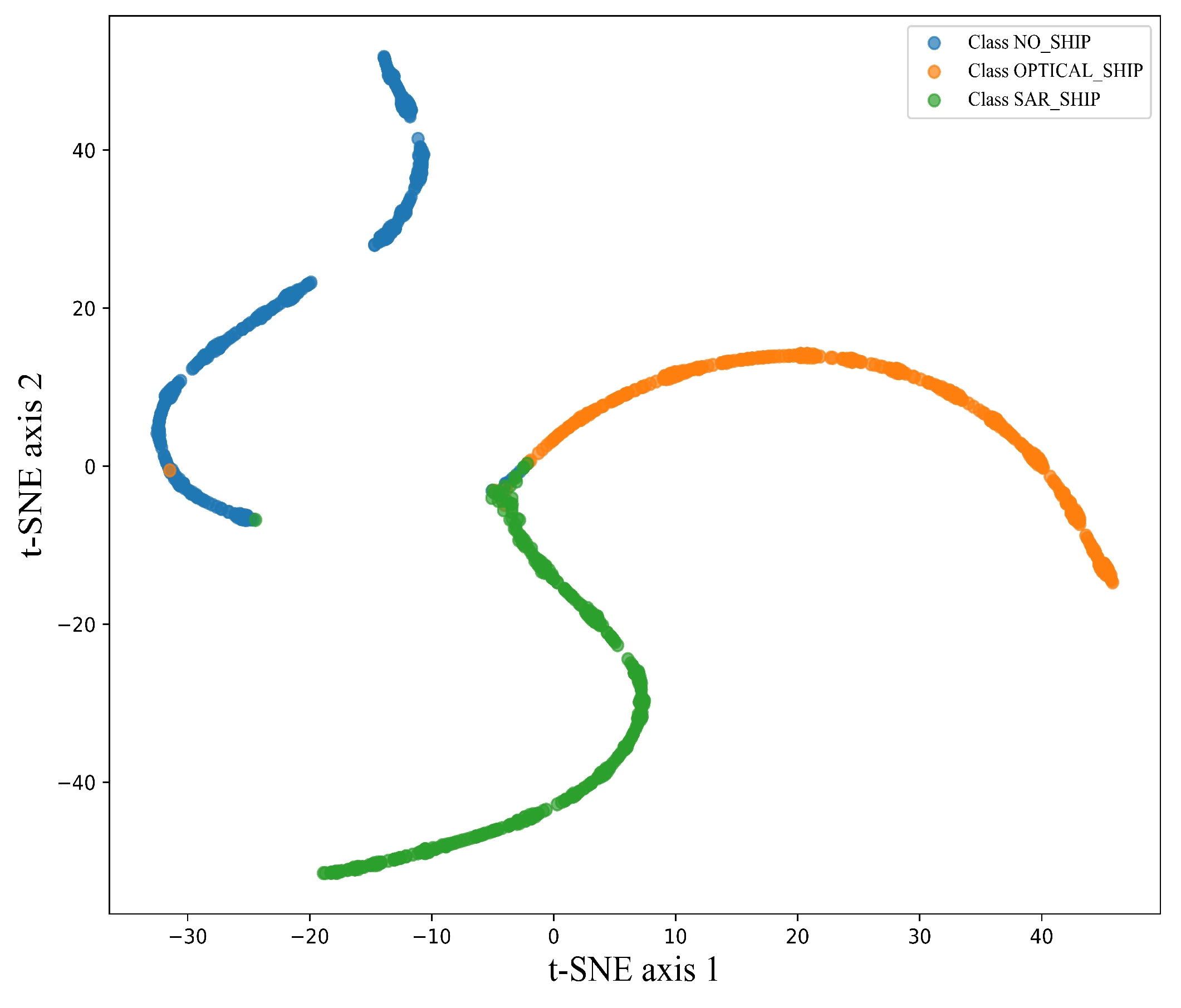
, on the same testing set. The confusion matrices in Figure 7 demonstrate reliable classification across all classes. The individual class performance under the Receiver Operating Characteristic (ROC) curve is graphically represented. The ROC curves in Figure 8 ((a) for SCABPNet and (b) for the Baseline + CBAM model) indicate robust discrimination ability. Figure 9 shows a t-SNE plot demonstrating how SCABPNet distinguished between the three classes with distinct feature clusters, proving its feature representation strength. 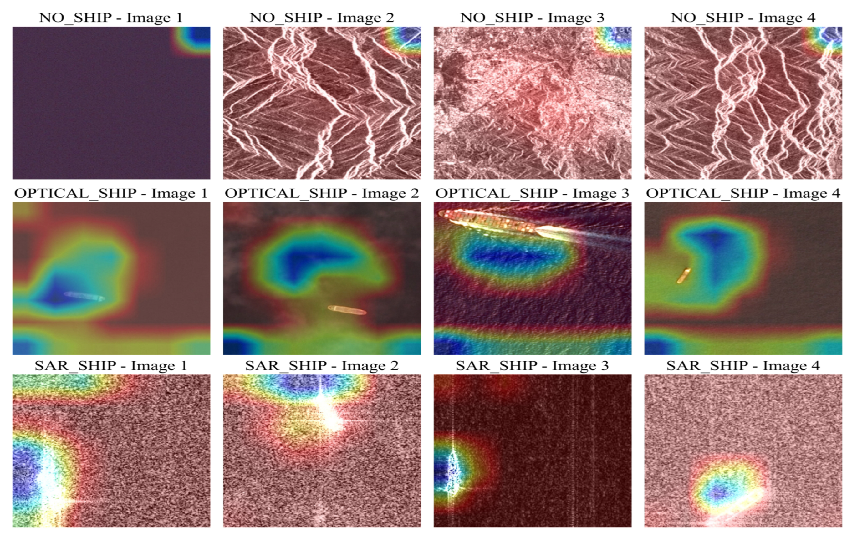Figure 10 displays SCABPNet’s attention heat maps on the test images, highlighting focus areas on ships and reducing background distractions, confirming the spatial–channel attention’s contribution to the model.

5.4. Experimental Results of SCABPNet under MSTAR Dataset

This section highlights the performance of our proposed SCABPNet model when applied to the well-known MSTAR dataset, a benchmark in the remote sensing field, comprising ten distinctive classes of military vehicles. The MSTAR dataset provides two distinct configurations: Standard Operating Conditions (SOCs) and Extended Operating Conditions (EOCs). For the scope of this investigation, we used the SOC configuration to evaluate the efficacy of SCABPNet in a 10-class classification scenario. The data partitioning of the MSTAR SOC configuration is presented in

Table 6. Description of Standard Operating Conditions (SOCs) training and testing sets with identical serial numbers and different depression angles (17° and 15°).

Classes	Serial Numbers	Training Set		Testing Set
		Depression	Samples	Depression	Samples
BMP_2	9563	17°	233	15°	195
BTR_70	C71	17°	233	15°	196
T_72	132	17°	232	15°	196
T_62	A51	17°	299	15°	273
BRDM_2	E71	17°	298	15°	274
BTR_60	b01k10yt7532	17°	256	15°	195
ZSU_23	d08	17°	299	15°	274
D_7	92v13015	17°	299	15°	274
ZIL_131	E12	17°	299	15°	274
2_S_1	b01	17°	299	15°	274

. Before presenting the results of this experiment, it is important to clarify that the primary objective behind this experiment was to test the proposed solution (SCABPNet) on a dataset that offers more than three classes. Therefore, the MSTAR dataset, renowned for comprising ten distinct categories, was suitable for this investigation. Furthermore, this experiment sought to discern the efficacy of SCABPNet when applied to homogeneous data, as well as its performance on datasets that do not have ship-specific features.

The evaluation of SCABPNet under MSTAR’s SOCs yielded highly impressive results, with accuracy, precision, recall, and F1-score metrics nearing the 98% mark, detailed in

Table 7. Overall performance of SCABPNet model on the MSTAR dataset.

	Precision	Recall	F1-Score	Support
2_S_1	0.9927	0.9927	0.9927	274
BMP_2	0.9788	0.9487	0.9635	195
BRDM_2	0.9926	0.9818	0.9872	274
BTR_60	0.9844	0.9692	0.9767	195
BTR_70	0.9795	0.9745	0.9770	196
D_7	0.9648	1.0000	0.9821	274
T_62	0.9926	0.9890	0.9908	273
T_72	0.9423	1.0000	0.9703	196
ZIL_131	0.9962	0.9672	0.9815	274
ZSU_23_4	0.9891	0.9891	0.9891	274
Overall	0.9813	0.9812	0.9811	2425
Accuracy			0.9823	2425
Macro avg	0.9813	0.9812	0.9811	2425
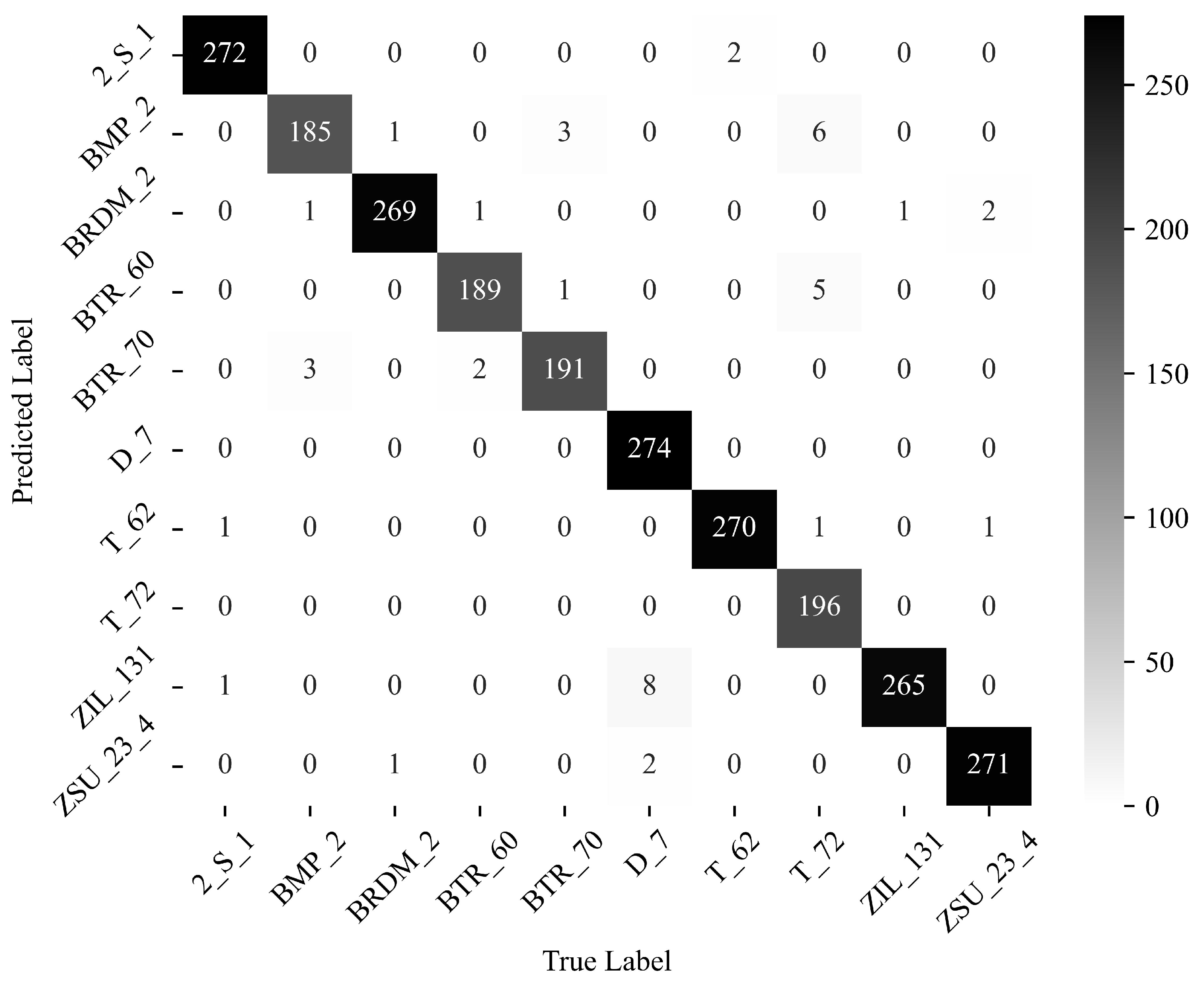
Weighted avg	0.9826	0.9823	0.9823	2425

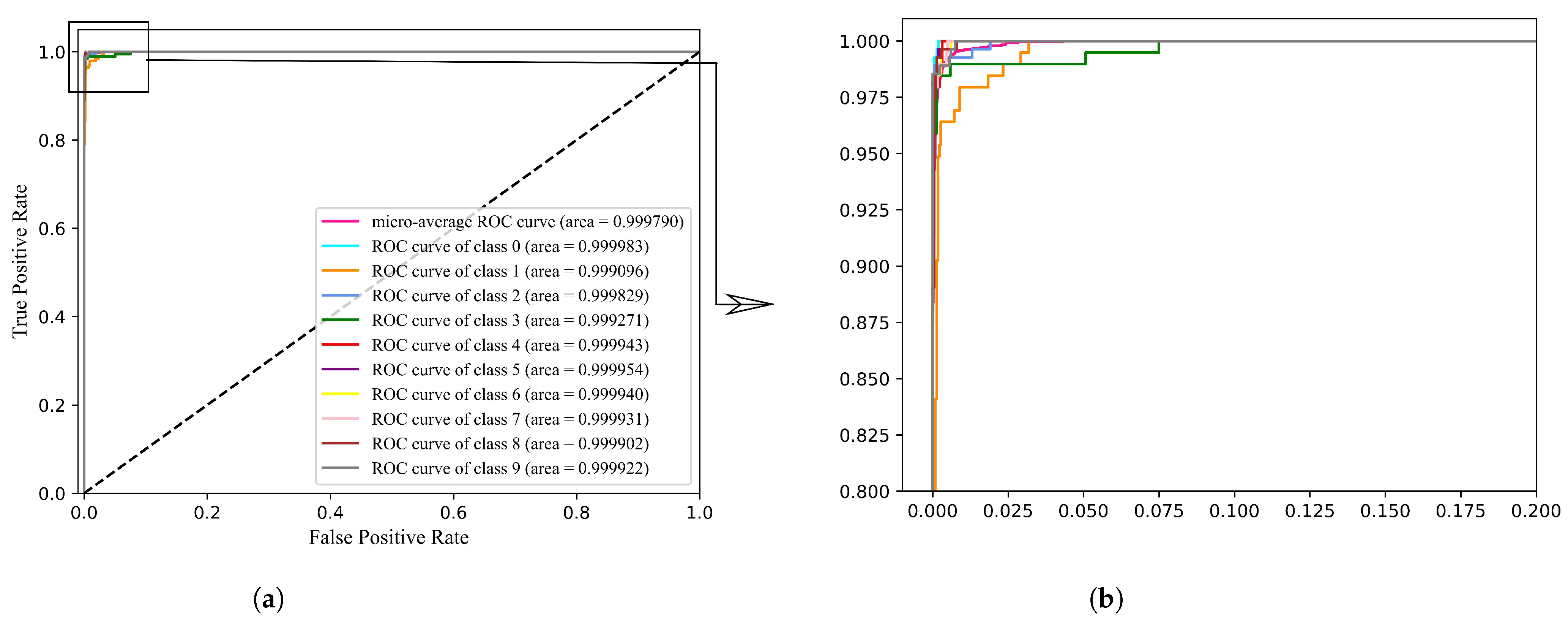
. The confusion matrix (Figure 11) showcases the model’s consistent performance, accurately classifying instances across a dataset of ten classes. Moreover, the class-specific ROC analysis, as presented in Figure 12, exhibited AUC scores surpassing 99.90%, underscoring SCABPNet’s exceptional capability to discern between classes with minimal error, thereby reinforcing its efficacy in handling varied and complex recognition scenarios.

5.5. Ablation Study

A comprehensive ablation study was conducted to validate the efficacy of some components within our proposed SCABPNet model. The primary objective was to evaluate the SCABP layer’s influence on the model’s overall performance. A comparative analysis was performed, juxtaposing the results derived from the SCABPNet model with the Baseline + CBAM model. As presented in Table 4 and Table 5, the integration of the SCABP layer consistently enhanced the classification metrics across all classes (SAR ship, optical ship, no ship) within the Heterogeneous Ship dataset. The ‘Baseline + CBAM’ column in

Table 8. Summary of the ablation study.

Class	Baseline + CBAM					Baseline + SCABP Layer
	Pre	Rec	F1	Acc	ROC/AUC	Pre	Rec	F1	Acc	ROC/AUC
SAR Ship	1	0.9000	0.9474	0.9000	0.9984	1	0.9545	0.9767	0.9545	0.9994
Optical Ship	0.9033	0.9909	0.9451	0.9909	0.9986	0.9426	0.9969	0.9690	0.9969	0.9997
No Ship	0.9698	0.9727	0.9713	0.9727	0.9982	0.9907	0.9787	0.9847	0.9787	0.9993
Overall	0.9577	0.9545	0.9546	0.9545	0.9984	0.9778	0.9767	0.9768	0.9767	0.9989

illustrates the performance metrics of the model using the CBAM approach. For the SAR ship class, the Baseline + CBAM model recorded an accuracy of 90%. Conversely, the ‘Baseline + SCABP layer’ column displays the results when the SCABP layer was incorporated into the model, which yielded significantly superior results. For the SAR ship, the accuracy escalated to 95.45%, indicating a substantial enhancement in all the performance metrics. A similar trend of improvement was observed for the optical ship and no ship classes, thereby reinforcing the effectiveness of the SCABP layer. As a result, the overall performance of the model also witnessed a significant improvement upon the inclusion of the SCABP layer. The precision improved from 95.77% to 97.78%, recall from 95.45% to 97.67%, F1-score from 95.46% to 97.68%, and accuracy from 95.45% to 97.67%. Moreover, the ROC/AUC values ranged from 0 to 1, with 1 indicating a perfect classification model. By incorporating the SCABPNet layer, the ROC/AUC of the proposed model increased from 99.47% to 99.89%.The SCABPNet model’s ROC/AUC was very close to 1, indicating an excellent performance in distinguishing between the classes.

Additionally, the confusion matrices of both models revealed that, in the proposed solution (SCABPNet), the SAR ship class had only 15 misclassifications, whereas the Baseline + CBAM model (CBAM approach) experienced 33 misclassifications. Moreover, when discriminating between the presence or absence of a ship, the SCABPNet model performed better than the Baseline + CBAM model. For example, within the SAR ship class, the SCABPNet model misclassified 13 images as the optical ship class when they were actually SAR ship class, and misclassified only 2 images as the no ship class. Conversely, the Baseline + CBAM model misclassified 7 images as the no ship class and 26 as the optical ship class. In summary, the confusion matrix of the proposed solution indicated a total of 3 images misclassified as the no ship class, while the Baseline + CBAM model’s confusion matrix showed 10 images in the no ship class. These findings suggest that the proposed solution is adept at accurately discriminating between ship images and no ship images. The results underscore the important role of the SCABP layer in enhancing the SCABPNet model’s performance. By facilitating more-effective feature extraction, the SCABP layer significantly improved the model’s ability to accurately classify different types of ships, emphasizing the SCABP layer’s importance in the proposed model.

5.6. Discussion

Handling heterogeneous data for classification tasks poses a significant challenge in the field of remote sensing. Our study addressed this issue, and the results presented in the previous section provided a comprehensive evaluation of the proposed SCABPNet model for this classification task. The model’s performance, as evidenced by the high precision, recall, F1-score, and accuracy, demonstrated its effectiveness in classifying different types of ships. This section discusses the implications of these results, the strengths and limitations of the study, and the potential directions for future research.

The SCABPNet model, with its novel Spatial–Channel Attention with Bilinear Pooling (SCABP) layer, showed a significant improvement in performance metrics over the Baseline + CBAM. The SCABP layer’s ability to apply spatial and channel attention mechanisms to the input data, followed by bilinear pooling, proved to be instrumental in enhancing the model’s performance. This was particularly evident in the ablation study, where the inclusion of the SCABP layer led to substantial improvements in all performance metrics across all classes within the Heterogeneous Ship dataset. This underscored the importance of the SCABP layer in facilitating more-effective feature extraction and, consequently, more-accurate ship classification.

When compared to other state-of-the-art methods, as shown in

Table 9. Overall metric comparison with other methods.

Methods	Accuracy	Precision	Recall	F1-Score
VGG-16 [3]	0.9306	0.9350	0.93	0.93
GBCNN [24]	0.8880	0.8804	0.8525	0.8661
SPAN [21]	0.9307	0.8186	0.7592	0.7866
ResNet-50 [41]	0.9093	0.9086	0.9101	0.9093
ResNet-50 [42]	0.9740	0.9079	0.9669	0.9364
ResNet-101 [43]	0.9620	0.9460	0.9320	0.9390
CNN-MR [44]	0.94	0.94	0.94	0.94
VGG16 [45]	0.9766	0.9785	0.9774	0.9779
Inception-V3 [45]	0.9548	0.9596	0.9535	0.9565
Cas-ShipNet [46]	0.9506	0.9707	0.9506	0.9506
ResNet-152 [47]	0.9135	0.9247	0.9135	0.9183
ResNet-152 [47]	0.9580	0.9583	0.9580	0.9581
R-CNN [48]	0.9725	0.9725	0.9731	0.9722
VGGNet [49]	0.8686	0.7397	0.8834	0.7791
ResNet-18 [49]	0.9707	0.9457	0.9761	0.9600
HOG-ShipCLSNet [50]	0.8669	0.8654	0.8662	0.8658
BANet [51]	0.950	0.9260	0.9330	0.9290
MetaBoost [52]	0.8101	0.7664	0.8090	0.7817
MetaBoost [52]	0.9099	0.9090	0.9083	0.9085
Heterogeneous CBAM (Ours)	0.9545	0.9577	0.9545	0.94546
Heterogeneous SCABPNet (Ours)	0.9767	0.9778	0.9767	0.9768

, the SCABPNet model demonstrated competitive performance. It outperformed most of the other methods in terms of the accuracy, precision, recall, and F1-score. Notably, it surpassed the performance of well-established models such as ResNet-50, ResNet-101, VGG-16, and Inception-V3, which have been recognized for their precision in numerous remote sensing applications. This indicates that our SCABPNet model, with its unique SCABP layer, is a promising tool for ship classification tasks, particularly in the context of Heterogeneous Ship data.

Additionally, we discuss the advantages and limitations of the proposed solution:

• Advantages of SCABPNet:
  Attention mechanism: The SCABPNet’s dual-attention mechanism (spatial and channel) allows it to concentrate on the most-salient features in both the spatial and channel dimensions. This helps eliminate redundant information, leading to more-accurate classifications.
  Bilinear pooling: By employing bilinear pooling, the SCABP layer can capture complex features and relationships between features, enhancing the model’s discriminative power.
  Robust performance: As demonstrated in the results, SCABPNet showed consistently superior performance across various performance metrics when compared to other state-of-the-art models. This indicates its effectiveness and potential applicability in real-world scenarios.
  Scalability: Given its modular nature, SCABPNet can be easily scaled up or integrated with other network architectures to further enhance performance or adapt to specific tasks.
• Limitations of SCABPNet:
  Generalizability: While SCABPNet demonstrated robust performance on the Heterogeneous Ship data, its performance on other maritime datasets or scenarios needs to be thoroughly evaluated.
  Computational complexity: The incorporation of the dual-attention mechanism and bilinear pooling augmented the computational demands, making SCABPNet more resource-intensive compared to simpler architectures.

The presented results in

Table 10. Comparison of FLOPs and accuracies with other models.

Models	FLOPs (G)	Accuracy (%)
MobileNetV3-Large [54]	0.16	95.93
FUSAR-CNN [53]	10.82	66.10
CNN [53]	0.11	76.70
VGG16_bn [29]	3.76	93.25
ResNet-50 [29]	5.38	96.50
SCABPNet (Our)	0.25	97.67

highlight the nuances and complexities of optimizing the computational cost and performance in ship data classification. The SCABPNet model demonstrated an exemplary balance between computational complexity and classification accuracy. With just 0.25 Giga Floating Point Operations Per Second (GFLOPs), SCABPNet outperformed notable architectures such as VGG16_bn and ResNet-50, achieving an accuracy of 97.67%. This clearly indicates the efficacy of the spatial–channel attention mechanism coupled with bilinear pooling in effectively classifying the Heterogeneous Ship data. Drawing comparisons with other models, the disparity in the FLOPs and accuracies showcased how more-complex models do not necessarily guarantee better performance. For instance, FUSAR-CNN, despite having the highest computational complexity at 10.82 GFLOPs, lagged behind with an accuracy of just 66.10% [53]. This stark contrast underscores the necessity of model optimization beyond just increasing the computational layers or nodes. When it comes to lightweight models, MobileNetV3-Large stood out with its efficiency, having a GFLOPs value of 0.16 and an accuracy of 95.93%.

To further evaluate the efficacy and robustness of SCABPNet, another experiment was conducted using the MSTAR dataset. The results of this experiment are depicted in Table 7 and Figure 11 and Figure 12. The results indicated that SCABPNet maintained good performance even when applied to a different dataset, notably one without ship features like the MSTAR dataset. Despite the inherent complexities associated with MSTAR data, the proposed model demonstrated high classification capabilities. The objective of this experiment was to showcase the ability of SCABPNet to effectively handle both homogeneous (MSTAR dataset) and heterogeneous datasets. Yet, an extensive evaluation of SCABPNet’s performance on various other datasets or in real-world scenarios is essential to ensure optimal recognition accuracy. Future work could involve testing the model on different datasets and in various real-world maritime scenarios to further validate its effectiveness and robustness. Another potential area for future research could be the investigation of the application of different attention mechanisms or pooling strategies within the SCABP layer. Although the existing implementation of the SCABP layer has demonstrated its effectiveness, exploring other attention or pooling strategies could potentially enhance the model’s performance.

6. Conclusions

The field of remote sensing has made significant advancements in the past decade due to increasing demands for improved performance. This study contributes to this ongoing progress by introducing SCABPNet, a novel spatial–channel attention with an improved bilinear pooling model specifically designed for the classification of Heterogeneous Ship data. Unlike previous studies that focused on homogeneous data, this work leveraged the complementary aspects of Synthetic Aperture Radar (SAR) and optical images, thereby enhancing the model’s performance. The SCABPNet model, with its unique SCABP layer, demonstrated superior performance in our experiments, surpassing the results of several deep learning models. The SCABP layer’s ability to effectively apply spatial and channel attention mechanisms followed by bilinear pooling proved instrumental in achieving these results. However, despite the promising results, it is important to acknowledge the challenges inherent in deep learning research, particularly in the context of radar and optical image analysis. The complexity of the parameters and dataset can lead to overfitting and long training times, requiring extensive training data. In light of these challenges, future work will focus on further improving the SCABPNet model and exploring new strategies to manage these variables. This includes extending the number of classes in the proposed ship dataset, investigating the ensemble learning of the proposed model for ship classification tasks, and exploring the use of other types of attention mechanisms and pooling methods. In conclusion, the SCABPNet model represents a significant step forward in ship classification, demonstrating the potential of combining SAR and optical images for enhanced performance. While challenges remain, this study provides a solid foundation for future research in this area, contributing to the ongoing advancement of maritime surveillance applications.

References

1. Xu, X.; Zhang, X.; Zhang, T. Lite-yolov5: A lightweight deep learning detector for on-board ship detection in large-scene sentinel-1 SAR images. Remote Sens. 2022, 14, 1018. [Google Scholar] [CrossRef]
2. Geng, J.; Jiang, W.; Deng, X. Multi-Scale Deep Feature Learning Network with Bilateral Filtering for SAR Image Classification. ISPRS J. Photogramm. Remote Sens. 2020, 167, 201–213. [Google Scholar] [CrossRef]
3. Xiong, G.; Xi, Y.; Chen, D.; Yu, W. Dual-polarization SAR ship target recognition based on mini hourglass region extraction and dual-channel efficient fusion network. IEEE Access 2021, 9, 29078–29089. [Google Scholar] [CrossRef]
4. Hong, Z.; Yang, T.; Tong, X.; Zhang, Y.; Jiang, S.; Zhou, R.; Han, Y.; Wang, J.; Yang, S.; Liu, S. Multi-scale ship detection from SAR and optical imagery via a more accurate YOLOv3. IEEE J. Sel. Top. Appl. Earth Obs. Remote Sens. 2021, 14, 6083–6101. [Google Scholar] [CrossRef]
5. Zhang, Y.; Guo, L.; Wang, Z.; Yu, Y.; Liu, X.; Xu, F. Intelligent ship detection in remote sensing images based on multi-layer convolutional feature fusion. Remote Sens. 2020, 12, 3316. [Google Scholar] [CrossRef]
6. Li, L.; Zhou, Z.; Wang, B.; Miao, L.; An, Z.; Xiao, X. Domain adaptive ship detection in optical remote sensing images. Remote Sens. 2021, 13, 3168. [Google Scholar] [CrossRef]
7. Firoozy, N.; Sandirasegaram, N. Tackling SAR imagery ship classification imbalance via deep convolutional generative adversarial network. Can. J. Remote Sens. 2021, 47, 295–308. [Google Scholar] [CrossRef]
8. He, J.; Wang, Y.; Liu, H. Ship classification in medium-resolution SAR images via densely connected triplet CNNs integrating fisher discrimination regularized metric learning. IEEE Trans. Geosci. Remote Sens. 2021, 59, 3022–3039. [Google Scholar] [CrossRef]
9. Sun, Z.; Meng, C.; Cheng, J.; Zhang, Z.; Chang, S. A multi-scale feature pyramid network for detection and instance segmentation of marine ships in SAR images. Remote Sens. 2022, 14, 6312. [Google Scholar] [CrossRef]
10. Cui, S.; Ma, A.; Zhang, L.; Xu, M.; Zhong, Y. MAP-Net: SAR and optical image matching via image-based convolutional network with attention mechanism and spatial pyramid aggregated pooling. IEEE Trans. Geosci. Remote Sens. 2022, 60, 1–13. [Google Scholar] [CrossRef]
11. Yang, X.; Zhang, H. Multi-source remote sensing data fusion and its applications: A comprehensive review. Int. J. Remote Sens. 2018, 39, 2251–2295. [Google Scholar]
12. Kanjir, U.; Greidanus, H.; Oštir, K. Vessel detection and classification from spaceborne optical images: A literature survey. Remote Sens. Environ. 2018, 207, 1–26. [Google Scholar] [CrossRef] [PubMed]
13. Rostami, M.; Kolouri, S.; Eaton, E.; Kim, K. Deep transfer learning for few-shot SAR image classification. Remote Sens. 2019, 11, 1374. [Google Scholar] [CrossRef]
14. Shakya, A.; Biswas, M.; Pal, M. Fusion and Classification of SAR and Optical Data Using Multi-Image Color Components with Differential Gradients. Remote Sens. 2023, 15, 274. [Google Scholar] [CrossRef]
15. Sreedhar, R.; Varshney, A.; Dhanya, M. Sugarcane Crop Classification Using Time Series Analysis of Optical and SAR Sentinel Images: A Deep Learning Approach. Remote Sens. Lett. 2022, 13, 812–821. [Google Scholar] [CrossRef]
16. Prabhakar, K.R.; Nukala, V.H.; Gubbi, J.; Pal, A.; P, B. Improving SAR and Optical Image Fusion for LULC Classification with Domain Knowledge. In Proceedings of the IGARSS 2022—2022 IEEE International Geoscience and Remote Sensing Symposium, Kuala Lumpur, Malaysia, 17–22 July 2022; pp. 711–714. [Google Scholar]
17. He, B.; Zhang, Q.; Tong, M.; He, C. Oriented Ship Detector for Remote Sensing Imagery Based on Pairwise Branch Detection Head and SAR Feature Enhancement. Remote Sens. 2022, 14, 2177. [Google Scholar] [CrossRef]
18. Xiong, W.; Xiong, Z.; Cui, Y. An explainable attention network for fine-grained ship classification using remote-sensing images. IEEE Trans. Geosci. Remote Sens. 2022, 60, 1–14. [Google Scholar] [CrossRef]
19. Zhao, Y.; Zhao, L.; Xiong, B.; Kuang, G. Attention receptive pyramid network for ship detection in SAR Images. IEEE J. Sel. Top. Appl. Earth Obs. Remote Sens. 2020, 13, 2738–2756. [Google Scholar] [CrossRef]
20. Hu, J.; Shen, L.; Albanie, S.; Sun, G.; Wu, E. Squeeze-and-excitation networks. In Proceedings of the IEEE Conference on Computer Vision and Pattern Recognition, Salt Lake City, UT, USA, 18–23 June 2018; pp. 7132–7141. [Google Scholar]
21. Sun, Y.; Wang, Z.; Sun, X.; Fu, K. SPAN: Strong Scattering Point Aware Network for Ship Detection and Classification in Large-Scale SAR Imagery. IEEE J. Sel. Top. Appl. Earth Obs. Remote Sens. 2022, 15, 1188–1204. [Google Scholar] [CrossRef]
22. Zhao, M.; Zhang, X.; Kaup, A. Multitask Learning for SAR Ship Detection with Gaussian-Mask Joint Segmentation. IEEE Trans. Geosci. Remote Sens. 2023, 61, 1–16. [Google Scholar] [CrossRef]
23. Li, E.; Samat, A.; Du, P.; Liu, W.; Hu, J. Improved bilinear CNN model for remote sensing scene classification. IEEE Geosci. Remote Sens. Lett. 2022, 19, 1–5. [Google Scholar] [CrossRef]
24. He, J.; Chang, W.; Wang, F.; Liu, Y.; Wang, Y.; Liu, H.; Li, Y.; Liu, L. Group bilinear CNNs for dual-polarized SAR ship classification. IEEE Geosci. Remote Sens. Lett. 2022, 19, 1–5. [Google Scholar] [CrossRef]
25. Lin, T.-Y.; RoyChowdhury, A.; Maji, S. Bilinear CNN models for fine-grained visual recognition. In Proceedings of the 2015 IEEE International Conference on Computer Vision (ICCV), Santiago, Chile, 7–13 December 2015; pp. 1449–1457. [Google Scholar]
26. Lin, T.-Y.; Maji, S. Improved bilinear pooling with CNNs. In Proceedings of the British Machine Vision Conference (BMVC), London, UK, 4–7 September 2017; pp. 117.1–117.12. [Google Scholar]
27. Lin, T.-Y.; RoyChowdhury, A.; Maji, S. Bilinear convolutional neural networks for fine-grained visual recognition. IEEE Trans. Pattern Anal. Mach. Intell. 2018, 40, 1309–1322. [Google Scholar] [CrossRef] [PubMed]
28. Li, X.; Lei, L.; Sun, Y.; Li, M.; Kuang, G. Multimodal Bilinear Fusion Network with Second-Order Attention-Based Channel Selection for Land Cover Classification. IEEE J. Sel. Top. Appl. Earth Obs. Remote Sens. 2020, 13, 1011–1026. [Google Scholar] [CrossRef]
29. Chen, W.; Gao, Y.; Chen, A.; Zhou, G.; Wang, J.; Yang, X.; Jiang, R. Remote sensing scene classification with multi-spatial scale frequency covariance pooling. Multimed. Tools Appl. 2022, 81, 30413–30435. [Google Scholar] [CrossRef]
30. Wang, Y.; Shi, H.; Chen, L. Ship detection algorithm for SAR images based on lightweight convolutional network. J. Indian Soc. Remote Sens. 2022, 50, 867–876. [Google Scholar] [CrossRef]
31. Hou, X.; Ao, W.; Song, Q.; Lai, J.; Wang, H.; Xu, F. FUSAR-ship: Building a high-resolution SAR-AIS matchup dataset of Gaofen-3 for ship detection and recognition. Sci. China Inf. Sci. 2020, 63, 1–19. [Google Scholar] [CrossRef]
32. Wang, N.; Wang, Y.; Er, M.J. Review on deep learning techniques for marine object recognition: Architectures and algorithms. Control Eng. Pract. 2020, 118, 104458. [Google Scholar] [CrossRef]
33. Wang, Y.; Wang, C.; Zhang, H.; Dong, Y.; Wei, S. A SAR dataset of ship detection for deep learning under complex backgrounds. Remote Sens. 2019, 11, 765. [Google Scholar] [CrossRef]
34. Kaggle. Dataset for Airbus Ship Detection Challenge. Available online: https://www.kaggle.com/c/airbus-ship-detection/overview (accessed on 21 August 2021).
35. Chen, Y.; Zheng, J.; Zhou, Z. Airbus ship detection-traditional vs. convolutional neural network approach. In CS299 Course Report; Stanford University: Stanford, CA, USA, 2020. [Google Scholar]
36. Tienin, B.W.; Cui, G.; Mba Esidang, R. Comparative ship classification in heterogeneous dataset with pre-trained models. In Proceedings of the 2022 IEEE Radar Conference (RadarConf22), New York, NY, USA, 21–25 March 2022; pp. 1–6. [Google Scholar]
37. Tienin, B.W.; Cui, G. A Convolutional Neural Network for Heterogeneous Ship Images Classification. In Proceedings of the 2021 CIE International Conference on Radar, Haikou, China, 15–19 December 2021; pp. 1004–1008. [Google Scholar]
38. Buades, A.; Coll, B.; Morel, J.-M. A non-local algorithm for image denoising. In Proceedings of the 2005 IEEE Computer Society Conference on Computer Vision and Pattern Recognition (CVPR’05), San Diego, CA, USA, 20–26 June 2005; Volume 2, pp. 60–65. [Google Scholar]
39. Xu, K.; Ba, J.; Kiros, R.; Cho, K.; Courville, A.; Salakhutdinov, R.; Zemel, R.S.; Bengio, Y. Show, attend and tell: Neural image caption generation with visual attention. In Proceedings of the 32nd International Conference on Machine Learning (ICML), Lille, France, 6–11 July 2015. [Google Scholar]
40. Woo, S.; Park, J.; Lee, J.-Y.; Kweon, I.S. CBAM: Convolutional block attention module. In Proceedings of the 2018 European Conference on Computer Vision (ECCV), Munich, Germany, 8–14 September 2018; pp. 3–19. [Google Scholar]
41. Gundogdu, E.; Solmaz, B.; Yücesoy, V.; Koç, A. MARVEL: A large-scale image dataset for maritime vessels. In Proceedings of the Computer Vision—ACCV 2016: 13th Asian Conference on Computer Vision, Taipei, Taiwan, 20–24 November 2016; Springer International Publishing: Berlin/Heidelberg, Germany, 2017; pp. 165–180. [Google Scholar]
42. Bao, W.; Huang, M.; Zhang, Y.; Xu, Y.; Liu, X.; Xiang, X. Boosting ship detection in SAR images with complementary pretraining techniques. IEEE J. Sel. Top. Appl. Earth Obs. Remote Sens. 2021, 14, 8941–8954. [Google Scholar] [CrossRef]
43. Li, D.; Liang, Q.; Liu, H.; Liu, Q.; Liu, H.; Liao, G. A novel multidimensional domain deep learning network for SAR ship detection. IEEE Trans. Geosci. Remote Sens. 2022, 60, 1–13. [Google Scholar] [CrossRef]
44. Bentes, C.; Velotto, D.; Tings, B. Ship classification in TERRASAR-X images with convolutional neural networks. IEEE J. Ocean. Eng. 2018, 43, 258–266. [Google Scholar] [CrossRef]
45. Wang, Y.; Wang, C.; Zhang, H. Ship classification in high-resolution SAR images using deep learning of small datasets. Sensors 2018, 18, 2929. [Google Scholar] [CrossRef] [PubMed]
46. Ucar, F.; Korkmaz, D. A novel ship classification network with cascade deep features for line-of-sight sea data. Mach. Vis. Appl. 2021, 32, 1–15. [Google Scholar] [CrossRef]
47. Leonidas, L.A.; Jie, Y. Ship classification based on improved convolutional neural network architecture for intelligent transport systems. Information 2021, 12, 302. [Google Scholar] [CrossRef]
48. Dechesne, C.; Lefèvre, S.; Vadaine, R.; Hajduch, G.; Fablet, R. Ship identification and characterization in sentinel-1 SAR images with multi-task deep learning. Remote Sens. 2019, 11, 2997. [Google Scholar] [CrossRef]
49. Domingos, L.C.F.; Santos, P.E.; Skelton, P.S.M.; Brinkworth, R.S.A.; Sammut, K. An investigation of preprocessing filters and deep learning methods for vessel type classification with underwater acoustic data. IEEE Access 2022, 10, 117582–117596. [Google Scholar] [CrossRef]
50. Zhang, T.; Zhang, X.; Ke, X.; Liu, C.; Xu, X.; Zhan, X.; Wang, C.; Ahmad, I.; Zhou, Y.; Pan, D.; et al. HOG-shipclsnet: A novel deep learning network with HOG feature fusion for SAR ship classification. IEEE Trans. Geosci. Remote Sens. 2022, 60, 1–22. [Google Scholar] [CrossRef]
51. Hu, Q.; Hu, S.; Liu, S. BANet: A Balance Attention Network for Anchor-Free Ship Detection in SAR Images. IEEE Trans. Geosci. Remote Sens. 2022, 60, 1–12. [Google Scholar] [CrossRef]
52. Zheng, H.; Hu, Z.; Liu, J.; Huang, Y.; Zheng, M. MetaBoost: A Novel Heterogeneous DCNNs Ensemble Network with Two-Stage Filtration for SAR Ship Classification. IEEE Geosci. Remote Sens. Lett. 2022, 19, 1–5. [Google Scholar] [CrossRef]
53. Zhang, Y.; Lei, Z.; Yu, H.; Zhuang, L. Imbalanced high-resolution SAR ship recognition method based on a lightweight CNN. IEEE Geosci. Remote Sens. Lett. 2022, 19, 1–5. [Google Scholar] [CrossRef]
54. Wang, C.; Luo, S.; Liu, L.; Zhang, Y.; Pei, J.; Huang, Y.; Yang, J. SAR ATR under limited training data via mobilenetv3. In Proceedings of the 2023 IEEE Radar Conference (RadarConf23), San Antonio, TX, USA, 1–5 May 2023; pp. 1–6. [Google Scholar]
Figure 1. Visualization of the proposed Heterogeneous Ship data (the SAR Ship class is marked in red, OPTICAL ship class marked in green, while the no ship class marked in blue).
Remotesensing 15 05759 g001
Figure 2. The flowchart of the proposed model for Heterogeneous Ship data classification: in red, we have the main components of the SCABP layer.
Remotesensing 15 05759 g002
Figure 3. The proposed spatial attention approach.
Remotesensing 15 05759 g003
Figure 4. The proposed channel attention approach.
Remotesensing 15 05759 g004
Figure 5. Architecture of the proposed SCABP layer.
Remotesensing 15 05759 g005
Figure 6. The training curves of the proposed model for Heterogeneous Ship data classification.
Remotesensing 15 05759 g006
Figure 7. Confusion matrices under Heterogeneous Ship data: (a) SCABPNet and (b) Baseline + CBAM.
Remotesensing 15 05759 g007
Figure 8. The Receiver Operating Characteristics (ROCs) under Heterogeneous Ship data: (a) SCABPNet and (b) Baseline + CBAM model.
Remotesensing 15 05759 g008
Figure 9. The t-SNE visualization of SCABP feature distribution.
Remotesensing 15 05759 g009
Figure 10. The attention mapping visualization of SCABPNet.
Remotesensing 15 05759 g010
Figure 11. Confusion matrix of SCABPNet on the MSTAR dataset.
Remotesensing 15 05759 g011
Figure 12. The ROC of SCABPNet on the MSTAR dataset: (a) normal view and (b) zoom view.
Remotesensing 15 05759 g012