Retrieval of Subsurface Velocities in the Southern Ocean from Satellite Observations

Abstract

Determining the dynamic processes of the subsurface ocean is a critical yet formidable undertaking given the sparse measurement resources available presently. In this study, using the light gradient boosting machine algorithm (LightGBM), we report for the first time a machine learning strategy for retrieving subsurface velocities at 1000 dbar depth in the Southern Ocean from information derived from satellite observations. Argo velocity measurements are used in the training and validation of the LightGBM model. The results show that reconstructed subsurface velocity agrees better with Argo velocity than reanalysis datasets. In particular, the subsurface velocity estimates have a correlation coefficient of 0.78 and an RMSE of 4.09 cm/s, which is much better than the ECCO estimates, GODAS estimates, GLORYS12V1 estimates, and Ora-S5 estimates. The LightGBM model has a higher skill in the reconstruction of subsurface velocity than the random forest and the linear regressor models. The estimated subsurface velocity exhibits a statistically significant increase at 1000 dbar since the 1990s, providing new evidence for the deep acceleration of mean circulation in the Southern Ocean. This study demonstrates the great potential and advantages of statistical methods for subsurface velocity modeling and oceanic dynamical information retrieval.

1. Introduction

Velocity is one of the most important variables in the ocean because of its relevance to global climate change, oceanic energy and nutrient transport, and marine ecosystem response in the face of greenhouse warming [1,2,3,4]. While the subsurface ocean contains the most complex dynamical processes, it is rather challenging to accurately determine their velocities. Recent research reveals a striking, deep-reaching acceleration in the global mean ocean circulation and offers a new perspective on understanding future ocean changes [5,6]. Whether the acceleration is deep is still controversial, as estimates of the global mean ocean circulation, especially the deep-sea circulation, remain highly uncertain due to changes in sampling and type of measurements as well as internal ocean variability [2,6,7]. The ability to directly measure subsurface velocity over large areas is still very limited. Subsurface in situ data are too sparse in time and space to accurately portray the ocean’s three-dimensional velocity, despite the fact that the global ocean velocity monitoring network is constantly supplied and enhanced. [8]. Hence, reconstructing subsurface velocity has important theoretical and practical implications.

Unlike prohibitively expensive in situ measurements, satellite remote sensing provides a cost-effective alternative for obtaining near-continuous global sea surface observations in space and time. However, direct ocean monitoring via satellite remote sensing is limited to the sea surface but ineffective in the oceanic subsurface [9]. Exploration of the subsurface ocean relies heavily on numerical simulations [5,10]. However, ocean numerical simulations face certain limitations in perfectly replicating real-world conditions [11,12]. The ocean’s subsurface velocities are dynamically linked to surface information [13,14,15]. Therefore, it is theoretically possible to reconstruct subsurface velocities from satellite observations. Nonetheless, it is essential to determine which and how such well-sampled sea surface observations can be used to retrieve the subsurface velocity [16,17].

Strategies for inferring subsurface velocities in the ocean from surface observations can be divided into two categories: dynamic and statistical. The dynamical method is mainly based on the conservation of potential vorticity (PV) or the surface quasi-geostrophic framework to establish the relationship between the surface information and the three-dimensional velocity of the ocean [13,14,15,18,19]. The subsurface velocity was calculated from the SQG framework based on the assumption that sea surface density and interior PV are closely related [18]. By combining interior decomposition with surface quasi-geostrophic (iSQG), a novel method for reconstructing ocean interior velocity was proposed [15]. The dynamic models disregard many complex dynamical processes in the real ocean and rely on idealized assumptions and boundary conditions. The reconstructed ocean subsurface velocities have also not been validated versus the measured velocities [13]. Therefore, the applicability of these models to the actual ocean remains subject to large uncertainties.

The statistical method has shown great promise in the reconstruction of three-dimensional fields of temperature and salinity [17,20,21]. However, statistical methods require many historical subsurface observations. Compared to temperature and salinity, subsurface velocities are measured much less frequently. In addition, the sea surface manifestation of the subsurface velocity is non-linear and complex [16,20]. It is governed by unidentified mechanisms. There are few reports on the use of statistical methods for the reconstruction of subsurface velocities.

The emergence of ARGO has made it possible to reconstruct ocean subsurface velocity based on statistical methods. As a result of the continuous deployment of Argo since 2000, the number of active floats has reached 4000 worldwide, generating approximately 150,000 observation profiles per year. Using the trajectory of the Argo, the Argo subsurface velocity at the depth of its parking can be calculated [22]. These accumulated large numbers of Argo subsurface velocities provide data support for the reconstruction of subsurface velocities using statistical techniques, especially machine learning techniques. Machine learning models frequently have unexpectedly high accuracy for simulating actual marine physical fields using data-driven empirical models that do not account for physical oceanography mechanisms [17,20].

This paper first proposes a statistical approach for retrieving subsurface velocities of the Southern Ocean (SO) from surface parameters (e.g., sea surface height, sea surface velocity, and sea surface wind) employing light gradient boosting machine (LightGBM) algorithms. To validate the applicability of the models to the actual ocean, the sea surface parameters and ocean subsurface velocities involved in their construction are derived from observational data. The sensitivity of the reconstructed velocity to different sea surface information is also evaluated. With the reconstructed model suggested by this study, the subsurface velocity was expanded to pre-Argo eras. We ultimately retrieved the SO velocities at 1000 dbar from 1993 to 2020 and analyzed their variations over the preceding nearly three decades.

2. Materials and Methods

2.1. Study Area and Data

The Southern Ocean, commonly defined as the ocean south of approximately 30°S, is an important sea connecting the Atlantic Ocean, the Indian Ocean, and the Pacific Ocean and has undergone pronounced subsurface warming, increasing anthropogenic carbon, and changes in oxygen over the past several decades [23]. Processes that act on local and regional scales, which are often mediated by the interaction of the flow with topography, are fundamental in shaping the large-scale, three-dimensional circulation of the Southern Ocean [24]. Due to the absence of land obstructions, the prevailing westerly wind of the Southern Ocean generates a powerful west-to-east circumpolar circulation, the Antarctic Circumpolar Current (ACC). The rapid zonal flow ACC induced by the combination of wind-induced circulation and thermohaline circulation contributes to the exchange of water mass between ocean basins, thereby promoting the transport of heat and energy [3,24]. The intensity of overturning circulation is also essential for regulating the exchange of anthropogenic heat at the sea surface and the redistribution of oceanic tracers [4,25]. Furthermore, the continuous transfer of energy from the atmosphere to the ocean increases the activity of eddies in the SO, which has implications for overturning circulation, carbon cycling, and climate change [26]. In order to understand ocean circulation and other dynamic processes in the context of recent global climate changes, precise measurements of the SO’s subsurface velocity are required. The SO between 30° and 60°S is selected as the study region due to the presence of ample in situ subsurface velocities for model training and a dynamic environment that is both complex and significant.

This study chose absolute dynamic topography (ADT), sea surface zonal velocity (SurZV), sea surface meridional velocity (SurMV), sea surface zonal wind (SurZW), and sea surface meridional wind (SurMW) as input parameters for LightGBM models to retrieve ocean subsurface velocity. ADT was obtained from the Archiving, Validation, and Interpretation of Satellite Oceanographic. The “twosat” delayed-time version of ADT was used due to its stable systematic error. SurMV and SurZV were obtained from the Physical Oceanography Distributed Active Archive Center’s (PO.DAAC) Ocean Surface Current Analyses Real-time (OSCAR) surface currents product. OSCAR surface currents are calculated using multi-source satellite observations and a simplified physical model of a turbulent mixed layer in the upper ocean. The OSCAR velocity consists of a geostrophic term, a wind-driven term, and a thermal wind adjustment [27]. Both AVISO and OSCAR offer products with a daily temporal resolution and a spatial resolution of 0.25 × 0.25°. In addition, SurZW and SurMW are daily surface vector wind products derived from NCEP-NCAR Reanalysis 1. The SurMV and SurZV were resampled to the same spatial grid as ADT via linear interpolation. All sea surface observations from 1993 to 2020 were collected. In situ subsurface velocity (SubZV and SubMV) obtained from the ARGO YoMaha’07 product of the Asia-Pacific Data Research Center was used to train and evaluate the LightGBM models. The velocities are estimated from the parking-level trajectories of the Argo floats. In particular, the estimation involved utilizing the final location and time on the sea surface from one cycle and the initial location and time from the next cycle. Via processing and quality control, YoMaha’07 products produce user-ready subsurface velocity datasets. And the mean error at the parking level is 0.53 cm/s, constituting approximately one-tenth of the mean velocity [22]. This dataset proves valuable for investigating eddy diffusivity [28] and examining regional dynamical states [29,30]. Here, the Argo velocities data spanning 2005 to 2020 at a parking pressure of 1000 dbar were collected.

To compare and evaluate the performance of the retrieved subsurface velocities, ocean subsurface velocity products from several reanalysis datasets were collected, including Global Ocean Data Assimilation System (GODAS) monthly reanalysis data with a resolution of 1° × 1°, Ocean Reanalysis System 5 (Ora-S5) monthly data with a resolution of 1° × 1°, Estimating the Circulation and Climate of the Ocean Version 4, Release 4 (ECCO hereafter) daily data with a resolution of 0.5° × 0.5°, and Global Ocean Physics Reanalysis (GLORYS12V1) daily data with a resolution of 0.0833° × 0.0833°. The datasets are widely used in mid-scale to long-scale ocean and climate change research [5,10]. We also employed the Argo monthly gridded velocity product provided by APDRC to quantify the precision of reconstructed velocity at large spatial and temporal scales.

2.2. Methods

Establishing mapping relationships between ocean subsurface velocity and sea surface measurements, which is essentially a process of developing regression models, is the primary objective of this study. In physical ocean field monitoring, regression, and prediction, machine learning is widely applied as a subfield of artificial intelligence [16,21]. Using the LightGBM method, we reconstructed the subsurface velocity in the SO over the past 30 years. The theory of LightGBM is introduced in Section 3.1. In Section 3.2, the procedure and experimental equipment for retrieving ocean subsurface velocity from satellite observations is described in detail.

2.2.1. Light Gradient Boosting Machine

LightGBM is an improved algorithm for gradient boosting decision trees (GBDT), proposed by Microsoft [31]. GBDT, an ensemble algorithm based on boosting, was proposed by Jerome Friedman [32]. GBDT links multiple decision trees in serial mode as opposed to parallel mode. Each decision tree is a weak learner. A new weak learner is generated to predict the error of the preceding weak learner. Thus, a strong learner with a small error is created by serializing the weak learners in each phase. Freidman [32] proposed using the negative gradient of the loss function to approximate the value of the loss for each tree. GBDT is applicable to both linear and non-linear regression issues. LightGBM, unlike the GBDT, applies the gradient-based one-side sampling (GOSS) algorithm to calculate the information gain by sampling various proportions of high- and low-gradient samples, allowing under-trained samples to receive more attention without compromising the model accuracy. LightGBM performs feature selection in the same manner. LightGBM utilizes a histogram-based decision tree algorithm to determine the optimal feature cutting point by discretizing and histogramizing the value of each feature, thereby requiring less computing memory and substantially increasing the computing speed without compromising precision. In addition, LightGBM abandons the level-wise strategy for layer-by-layer tree growth in favor of the leaf-wise algorithm for leaf-by-leaf tree growth. The level-wise strategy entails splitting all nodes in each layer, which incurs superfluous complexity as a result of the split of nodes with lesser gains, whereas the leaf-wise growth strategy selects the node with the greatest profit to split among all leaf nodes. In situations with the same number of splits, the leaf-wise method can also reduce errors. To prevent trees from growing indefinitely, the LightGBM parameter max_depth, which limits the maximum depth of the decision tree, is also defined. These innovative enhancements to LightGBM greatly decrease the model’s computational time and memory requirements, making it a popular choice for industrial applications.

In addition, random forest (RF) and multiple linear regression (MLR) were employed as comparative methods. RF is an extension of the bagging strategy of ensemble learning. It primarily employs replacement sampling to train multiple parallel base learners and integrates the results of multiple base learners to predict the model’s ultimate outcome. The hyperparameters of RF to be trained are the number of trees in the forest and the number of variables or features in the random subset at each node, neither of which is typically very sensitive to its value [33].

Scikit-learn is a Python module that integrates a wide range of state-of-the-art machine learning algorithms [34]. We can directly call a variety of machine learning regression modules to build models with simple procedures. In view of its usability and high performance, the Scikit-learn Python module is deployed to construct the LightGBM models that derive the ocean subsurface velocity from sea surface parameters.

2.2.2. Experimental Setup

Figure 1 depicts the flowchart for retrieving the subsurface velocity of the SO at 1000 dbar using the LightGBM method. Before model training, the dataset for ocean subsurface velocity reconstruction was established with the surface components (i.e., ADT, SurZV, SurMV, SurZW, and SurMW) and location components (Longitude, referred to as Lon, and Latitude, referred to as Lat) as model inputs and the ARGO at 1000 dbar (SubZV and SubMV) as model outputs. Notably, trigonometric transformations were applied to establish continuous spatial relationships in the position component. Due to the fact that the ARGO YoMaHa’07 subsurface velocity is a set of estimates at random times and locations, the sea surface observations closest in space-time to the Argo subsurface velocities were selected as its matching model inputs. The dataset contains 413,949 records from 2005 to 2020. All records were linearly normalized to [−1 1] and divided into a training dataset (2010–2020, 322,363 records) and a validation dataset (2005–2009, 91,586 records).

Some of the model parameters cannot be derived directly through training, necessitating optimization of hyperparameters prior to training. The applicable hyperparameters can substantially enhance the model’s accuracy. Here, we optimized the model’s hyperparameters using a Bayesian optimization technique with the training dataset. Bayesian optimization obtains optimal hyperparameters by fitting a Gaussian distribution of the hyperparameter space iteratively with continuously updated prior knowledge [35]. The primary objective of parameter optimization is to acquire a highly accurate model without overfitting or underfitting as quickly as possible.

Table 1. The meaning and value of optimal hyper-parameters for the LightGBM model to estimate SubMV and SubZV in the SO.

Hyperparameters	Meaning	Optimal Values
		SubZV/SubMV
learning_rate	Shrinking the weights on each step	0.028/0.005
num_leaves	The maximum number of leaf nodes in the tree	280/90
max_depth	The maximum depth of a tree	19/20
min_data_in_leaf	The minimum number of records a leaf may have	39/22
bagging_fraction	The fraction of data used at each iteration	0.5/0.5
feature_fraction	The fraction of feature used at each iteration	0.8/0.7
lambda_l1	L1 regularization term on weights	0.95/0.9
lambda_l1	L2 regularization term on weights	0.95/0.1
max_bin	The maximum number of bins to store features	297/279

displays the values and interpretations of the crucial hyperparameters of the Bayesian-optimized LightGBM models. The purpose of learning_rate is to regulate the learning rate for searching hyperparameters. A small learning_rate produces more precise models, but at the expense of the additional time required for hyperparameter optimization. The parameters num_leaves, min_data_in_leaf, and max_depth are used to control the complexity of the model structure. Large or small values of num_leaves and min_data_in_leaf may result in overfitting or underfitting. The bagging_fraction and feature_fraction represent the proportions of sample and feature sampling during each iteration, respectively. Diminishing these two parameters can prevent model overfitting and speed up the calculation. However, if these two parameters are set too low, the model will not be able to fully account for the diversity of data and features in training, leading to a decrease in model performance. The regularization parameters lambda_l1 and lambda_l2 are determined to reduce overfitting. In addition, a five-fold cross-validation in chronological order with the training dataset was used for robust hyperparameters.

Then, we trained the LightGBM model equipped with the optimal hyperparameters using all training records and determined the model’s accuracy by calculating the error on the validation dataset. The root mean squared error (RMSE) and correlation coefficient were employed to quantitatively evaluate the reconstructed ocean subsurface velocities. A low RMSE and high r indicated superior model performance with higher reconstruction accuracy. We eventually retrieved the SO’s subsurface velocity (SubZV and SubMV) at 1000 dbar from 1993 to 2020 based on sea surface observations and location information using the trained LightGBM model. The retrieved ocean subsurface velocities correspond to the spatial and temporal resolution of the surface satellite parameters, i.e., a spatial resolution of 0.25° × 0.25° and a temporal resolution of one day. Due to the paucity of subsurface observations for LightGBM model reconstruction at other depths, the subsequent analysis and evaluation of the reconstructed ocean subsurface velocity will be restricted to 1000 dbar.

3. Results and Discussion

3.1. Model Determination

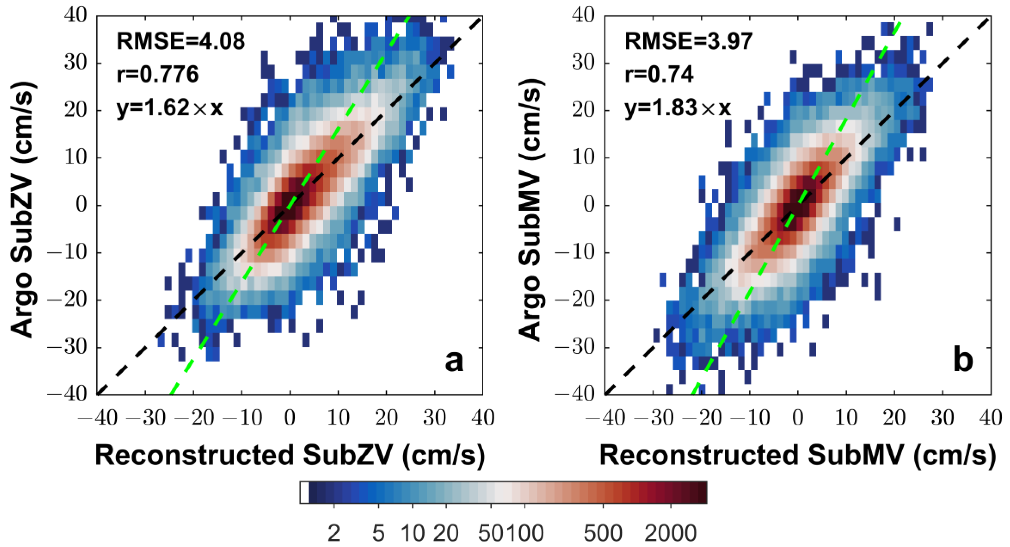
To achieve higher accuracy in constructing a machine learning model, it requires careful consideration for the selection of not only the advanced algorithms but also the suitable input parameters for the model [17,21]. As shown in

Table 2. The performance comparison of different cases on reconstructing SubMV and SubZV by employing RMSE and r.

Cases	Model	Input Parameters	RMSE (cm/s)/r (%)
			SubZV	SubMV
Case 1	Lightgbm	SurZV, SurMV, ADT, Lat, Lon, SurZW, SurMW	4.08/77.6 (0.11 *)	3.97/74.0 (0.29 *)
Case 2	Lightgbm	SurZV, SurMV, ADT, Lat, Lon	4.12/77.0 (0.24 *)	4.03/73.1 (0.36 *)
Case 3	Lightgbm	SurZV, SurMV, Lat, Lon, SurZW, SurMW	4.13/77.0 (0.24 *)	4.00/73.6 (0.40 *)
Case 4	Lightgbm	SurZV, SurMV, ADT, SurZW, SurMW	4.35/74.1	4.16/71.0
Case 5	Lightgbm	ADT, Lat, Lon, SurZW, SurMW	5.59/50.3	5.56/34.1
Case 6	RF	SurZV, SurMV, ADT, Lat, Lon, SurZW, SurMW	4.14/76.9 (0.03 *)	4.02/73.2 (0.03 *)
Case 7	MLR	SurZV, SurMV, ADT, Lat, Lon, SurZW, SurMW	4.43/72.8	4.23/0.70

* This uncertainty was estimated by repeating the training and testing procedures 10 times and calculating the two standard deviations of the r (which correspond to the 95% confidence interval).

, seven cases with various algorithms or parameter combinations were designed to determine the optimal model for estimating ocean subsurface velocity. We performed separate constructions of SubZV and SubMV estimated models using the configurations from the seven cases and then measured their accuracy on the validation dataset with the correlation coefficient and RMSE. In Case 1, the LightGBM model in conjunction with the input parameters of SurZV, SurMV, ADT, Lat, Lon, SurMW, and SurZW yields the best reconstructed results across all cases. Specifically, the model attains an RMSE of 4.08 cm/s, a correlation coefficient of 0.776 for SubZV, an RMSE of 3.97 cm/s, and a correlation coefficient of 0.74 for SubMV. The 2D histogram graph between the reconstructed subsurface velocity in Case 1 and the Argo velocity in the validation dataset is shown in Figure 2. The color of each grid cell (cells hereafter) corresponds to the number of subsurface velocity pairs that are present within that cell, with blue indicating a small number and red indicating a large number. The high-intensity cells are clustered along the equal-value line (represented by a black dashed line). This indicates a strong positive correlation for both the SubZV and the SubMV estimated by Case 1 relative to the Argo measurements. Consistent with the velocity measured by Argo, both the reconstructed SubMV and SubZV generally ranged between −40 and 40 cm/s. Additionally, the cells close to zero had the highest intensity. This indicates that the majority of velocities at depths of 1000 dbar in the SO are relatively weak, and estimating such weak subsurface velocities is extremely difficult. As a result, the dispersion between the Argo velocity and the reconstructed velocity is greater for the small velocity component compared to the large velocity component in Figure 2. It is worth noting that the slope of the fit lines (indicated by green dotted lines) between the reconstructed SubZV and SubMV and the Argo velocity is greater than the slope of their equal-value line (diagonal line), indicating that the reconstructed velocity is underestimated relative to the Argo velocity. The reasons behind this underestimation can be multifaceted. One possible cause could be the fact that the area of the surface satellite’s data grid points (~25 km) is relatively large, and the area of the grid points corresponding to the reconstructed subsurface velocity is similarly large, which is equivalent to smoothing out the small-scale velocity, resulting in a smaller velocity, whereas the spatial scale corresponding to the Argo subsurface velocity is smaller, which may be the reason why the reconstructed velocity is underestimated relative to the Argo velocity.

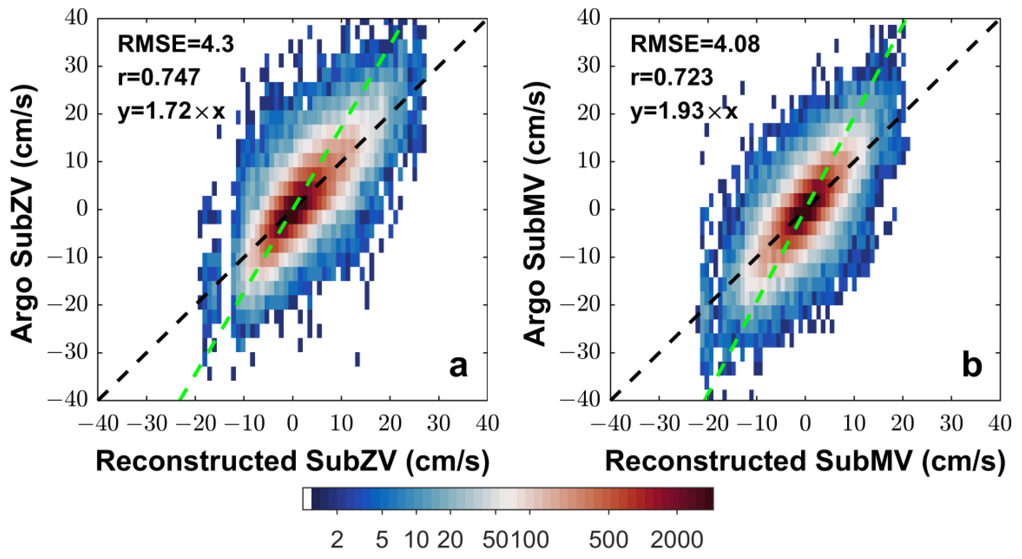
The results of Case 2 through Case 5 presented in Table 2 show a statistically significant decrease in the accuracy of LightGBM models, regardless of which input parameter from Case 1 was removed. This suggests that each input parameter in Case 1 contributes positively to enhancing the accuracy of subsurface velocity estimation. For example, wind can provide energy for the ocean’s general circulation. In addition, the response of ocean surface observations to subsurface velocities is spatially heterogeneous, which implies that this response is related to geographic location information. This assertion is supported by the fact that Case 4, which does not include geographic location parameters (Lat and Lon) as inputs, exhibits apparently inferior performance compared to Case 1. In comparison to the other cases, the accuracy of Case 5 exhibits the most notable decrease due to the exclusion of the input parameters of surface velocity (SurMV and SurZV). This is supported by the largest RMSE of 5.56 cm/s and 5.59 cm/s and the smallest correlation coefficients of 0.341 and 0.503 for the reconstructed SubMV and SubZV. The worst performance in Case 5 indicates that surface velocity is essential to estimating the subsurface velocity in the SO. Geostrophic currents consist of barotropic and baroclinic components. The barotropic component remains constant regardless of depth, whereas the baroclinic component diminishes progressively with increasing depth [36,37]. Thus, the surface velocity is strongly correlated with the subsurface velocity, particularly in the presence of strong geostrophic currents. This accounts for the dominant role of surface velocity in estimating subsurface velocity in the SO. However, it is worth noting that Case 5 produces such poor results despite the fact that its input parameters include ADT, latitude, and longitude and these parameters can provide accurate estimates of geostrophic velocity. We replaced ADT, latitude, and longitude in Case 5 with geostrophic velocity (here denoted by Case 8), and calculated the reconstructed velocity of Case 8. As shown in Figure 3, the accuracy of the reconstructed SubZV and SubMV shows a large discrepancy compared to that of Case 5. This suggests that the machine learning model cannot directly extract the geostrophic velocity from ADT and latitude. For machine learning, the more direct the relationship between input and output parameters, the easier it is for machine learning to capture them, and vice versa. In addition, the results of Case 8 are more similar to those of Case 1, which demonstrates that the geostrophic velocity component in the OSCAR current contributes significantly to the reconstruction of the subsurface velocity. In brief, the combinations of input parameters including SurZV, SurMV, ADT, Lat, Lon, SurZW, and SurMW are optimal for reconstructing subsurface velocity in the SO.

In the comparative analysis of Case 1, Case 6, and Case 7, it was observed that the LightGBM model with the optimal input parameter combination significantly outperformed both the RF model and the MLR model with the same input parameters. It is noteworthy that the RMSE values for the subsurface SubZV and SubMV estimated through the conventional MLR model are considerably greater than the RMSE of the reconstructed subsurface velocity obtained through the LightGBM model. This is because the variability of mesoscale eddy dynamic processes, which account for the greater proportion of kinetic energy in the entire ocean, is basically non-linear in the actual ocean [38]. According to [20], MLR models are significantly less capable than machine learning models at fitting non-linear associations between input and output parameters. Due to the difficulty in capturing these non-linear dynamic processes, the MLR estimates ocean subsurface velocities with less precision. In conclusion, based on the performance of the seven cases, the LightGBM model with the optimal combination of input parameters (Case 1) was selected for estimating the ocean subsurface velocity in the SO.

3.2. Comparisons with Reanalysis Data

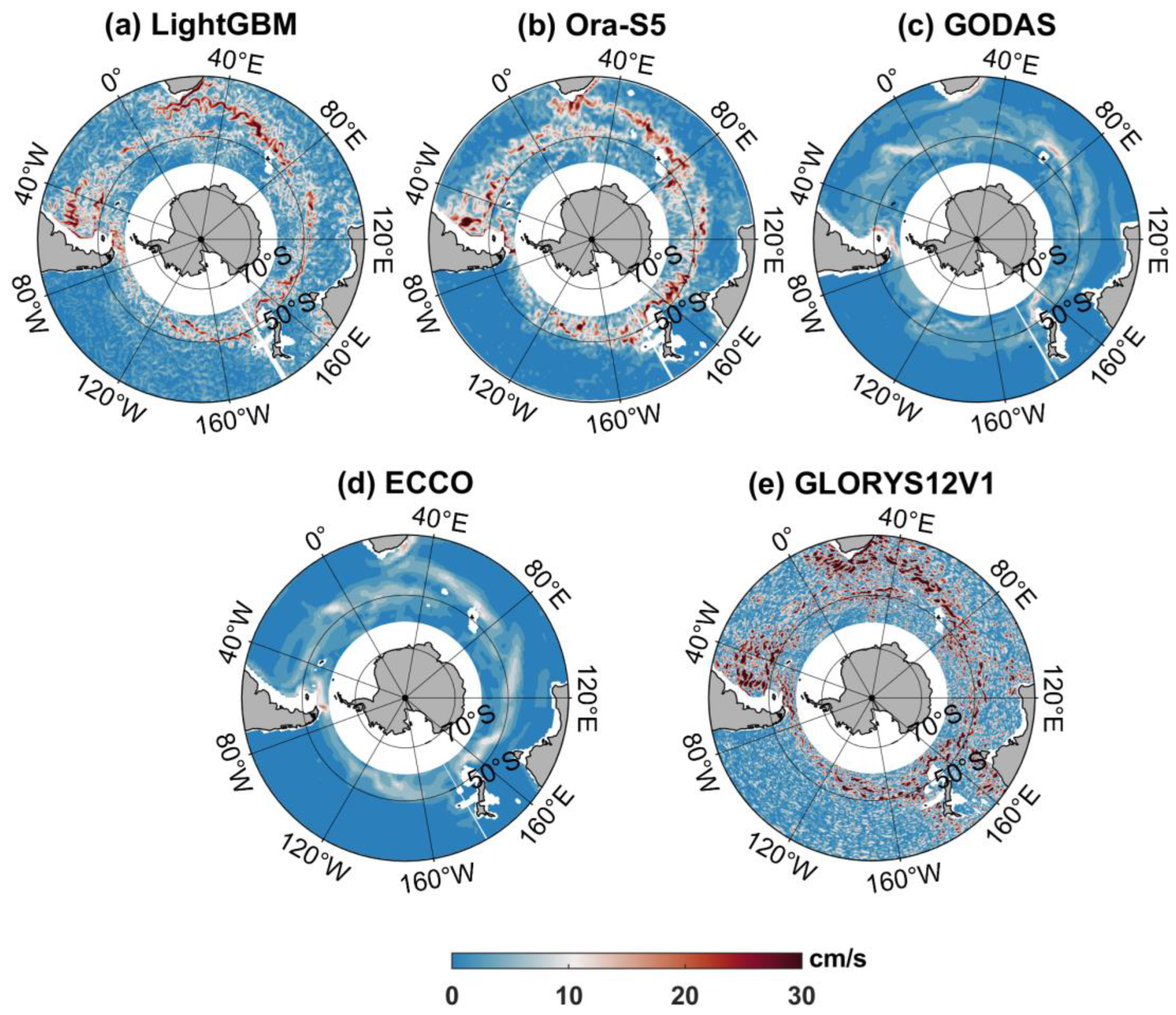
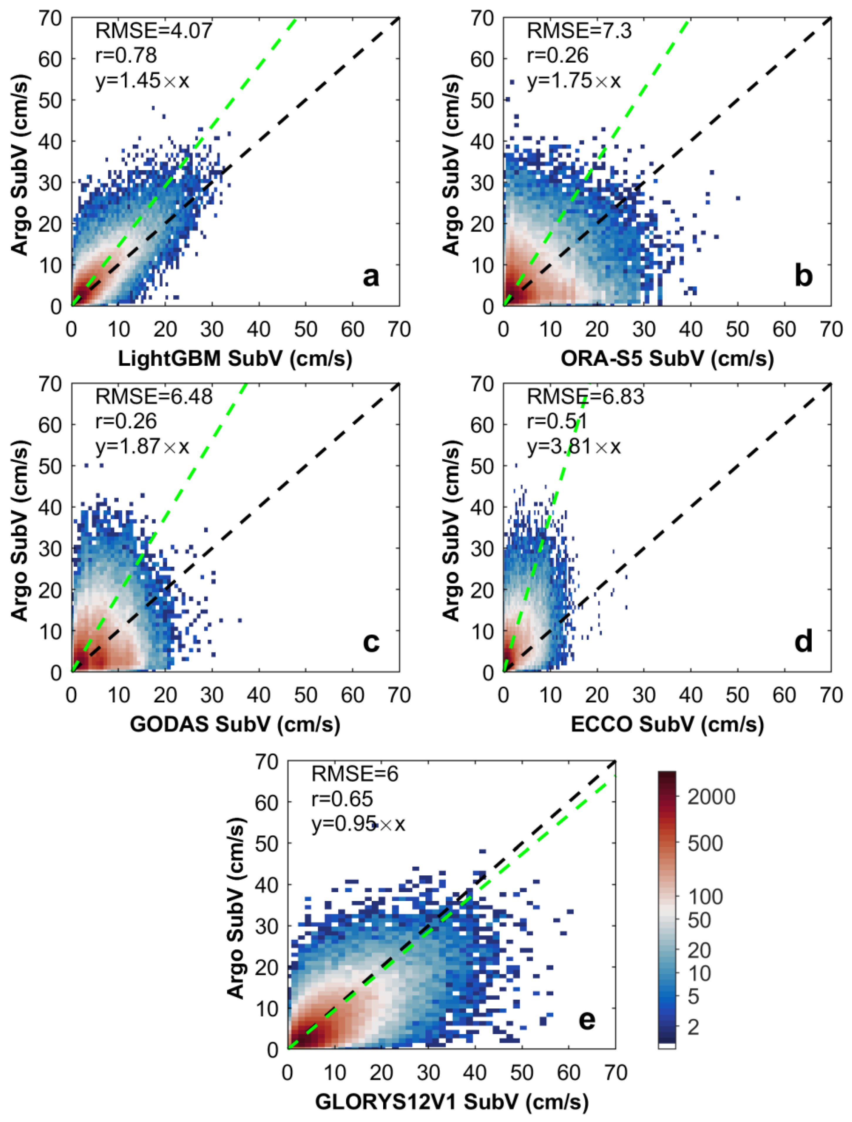
Figure 4a displays the magnitude of the LightGBM subsurface velocity (SubV) for the SO based on Case 1 SubZV and SubMV. Furthermore, as comparisons, the SubV of Ora-S5, GODAS, ECCO, and GLORYS12V1 are shown in Figure 4b–e. LightGBM SubV characterizes the Southern Ocean current field with greater detail than the GODAS SubV and ECCO SubV due to its superior spatial and temporal resolution. Additionally, in the LightGBM SubV, the Antarctic Circumpolar Current can be seen more distinctly than in the SubV of the two reanalysis datasets. Similar to the LightGBM SubV, the Ora-S5 and GLORYS12V1 SubV also display the ACC in a clear manner. To quantitatively compare the performance of the SubV for the LightGBM, Ora-S5, GODAS, ECCO, and GLORYS12V1, we computed the correlation coefficient and RMSE between the SubV of the five datasets and the ARGO SubV on the validation dataset. The SubVs of Ora-S5, GODAS, ECCO, and GLORYS12V1 that are the closest to the ARGO SubVs of the validation dataset in time and space were chosen. The 2D histograms between LightGBM SubV, Ora-S5 SubV, GODAS SubV, ECCO SubV as well as GLORYS12V1 SubV, and Argo SubV are shown in Figure 5, respectively. The high-density grid cells of the LightGBM SubV are relatively closer to the equal-value line compared to those of the Ora-S5 SubV, GODAS SubV, ECCO SubV, and GLORYS12V1 SubV. In quantitative terms, the LightGBM SubV stands out with a correlation coefficient of 0.78 and a root mean square error (RMSE) of 4.08 cm/s. This performance surpasses that of the Ora-S5 SubV, which has a correlation coefficient of 0.26 and an RMSE of 7.3 cm/s, the GODAS SubV with a correlation coefficient of 0.26 and an RMSE of 6.48 cm/s, the ECCO SubV with a correlation coefficient of 0.26 and an RMSE of 6.48 cm/s, and the GLORYS12V1 SubV with a correlation coefficient of 0.65 and an RMSE of 6.0 cm/s. The correlation coefficient between Ora-S5 SubV, GODAS SubV, ECCO SubV, GLORYS12V1 SubV, and Argo SubV are relatively low. It is understandable that models usually provide a statistical approximation of ocean conditions at a given time rather than the actual conditions at that time. The better quantitative performance of the LightGBM model indicates that our reconstructed velocities provide more accurate estimates of absolute subsurface velocity in the real ocean than the reanalysis model does. Notably, similar to the reconstructed SubZV and SubMV in Figure 2, the fit lines (indicated by green dotted lines) between the LightGBM SubV, Ora-S5 SubV, GODAS SubV, ECCO SubV, and GLORYS12V1 SubV and the Argo SubV deviate from their equal-value lines in Figure 5. The difference in resolution between the SubV of the five datasets and the Argo SubV may also contribute to this discrepancy.

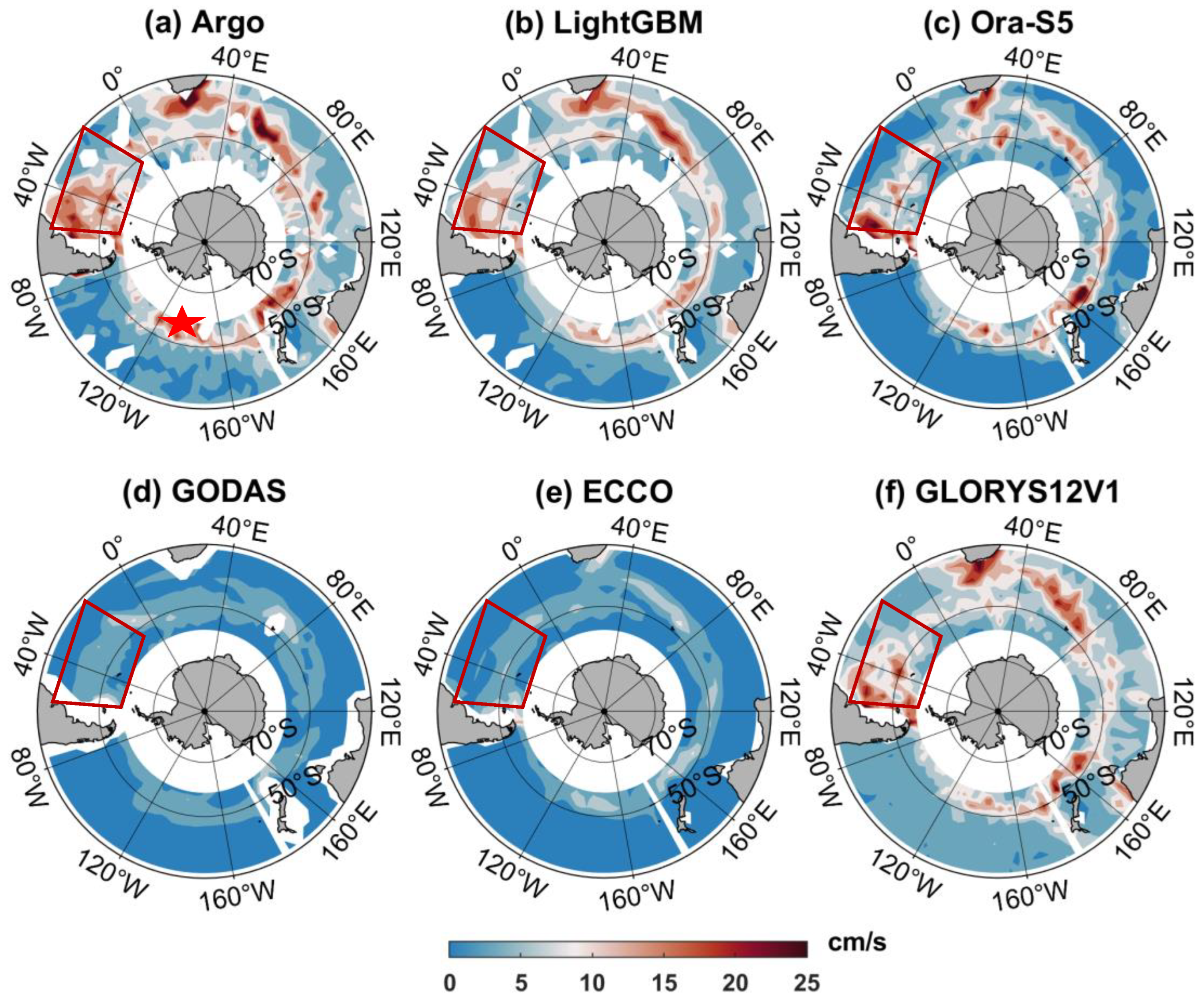
In addition to comparisons at the mesoscale, the large-scale velocity field characteristics of the LightGBM SubV were compared with those of the SubV from the reanalysis datasets. We employed the annual gridded Argo SubV, derived from the annual average of monthly grid Argo products with a 3° spatial resolution, to evaluate the accuracy of the LightGBM SubV on a large scale. And we used the spatial-temporal averaging method to unify the spatial-temporal resolution of the LightGBM SubV to be consistent with the Argo annual grid product. That is, LightGBM annual SubV is obtained by equal-weighted averaging of the estimated daily SubV within the spatial-temporal range of each grid in the Argo annual grid product. The ECCO SubV, Ora-S5 SubV, GLORYS12V1 SubV, and GODAS SubV were also selected as comparisons, and the annual SubV of those four datasets was obtained by the same computational procedure as the LightGBM annual SubV. Figure 6 depicts the map of the annual SubV for the six datasets in 2009. From the perspective of the overall spatial distribution characteristics of the SO, the annual SubV of Ora-S5, GLORYS12V1, and LightGBM show a strong visual cohesion with the Argo annual SubV, thereby presenting the spatial distribution characteristics of the Antarctic Circumpolar Current more clearly, whereas the GODAS annual SubV and the ECCO annual SubV present a much weaker Antarctic Circumpolar Current and lack many detailed features. In addition, the flow field characteristics in local regions, such as the west coast of the Atlantic (red box), the Argo, GLORYS12V1, and LightGBM annual SubV exhibit an annular current characteristic, surrounded by the Falkland cold current and the western boundary current. However, the annual SubV of ECCO, GODAS, and Ora-S5 lack such current features of the Argo annual SubV.

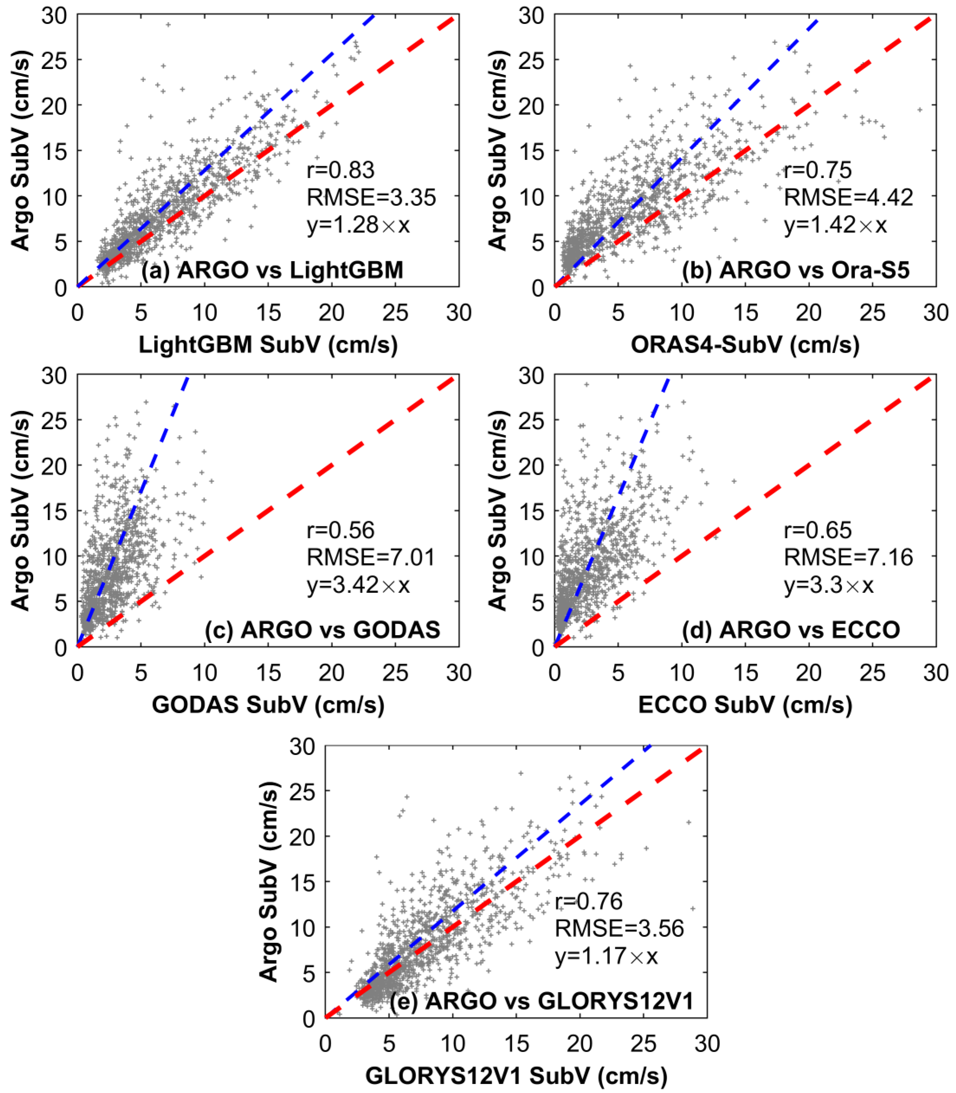
We also calculated the correlation coefficient and the RMSE for the LightGBM, Ora-S5, GODAS, GLORYS12V1, and ECCO annual SubV versus the annual Argo SubV in 2009 separately. As shown in Figure 7, LightGBM annual SubV (r = 0.83, RMSE = 3.35 cm/s) has a much better performance than Ora-S5 annual SubV (r = 0.72, RMSE = 4.67 cm/s), GODAS annual SubV (r = 0.56, RMSE = 7.01 cm/s), GLORYS12V1 annual SubV (r = 0.76, RMSE = 3.56 cm/s), and ECCO annual SubV (r = 0.66, RMSE = 7.2 cm/s). Note that for the annual SubV of these five datasets, the slope of their fit line is higher than that of their equal-value line, i.e., the annual SubV of these five datasets is also underestimated in terms of the Argo annual SubV. The annual SubV of ECCO and GODAS are more underestimated, which can also be drawn from their apparently lighter shade in Figure 6d,e. Also, the performance of the LightGBM SubV at a large scale is superior to that at a small scale with a higher accuracy (comparison of Figure 5a and Figure 7a), indicating that the LightGBM SubV is more accurate in describing large-scale velocities.

To further validate LightGBM SubV, we compared the consistency of LightGBM SubV and the different datasets with ARGO during the period 2005–2009. Due to the limited spatial and temporal coverage of ARGO in the SO during the period 2005–2009, we chose the ARGO monthly SubV of six sites (the center of a 3 × 3 degree area) with relatively abundant observations for comparison. Figure 8 shows the time series of the monthly SubV from ARGO, LightGBM, OraS5, GODAS, ECCO, and GLORYS12V1 spanning 2005 to 2009 at 49.5°S and 127.5°W. Despite the differences in the inter-month variability, the 12-month low-pass filtered series of ARGO and LightGBM monthly SubV exhibit high consistency at this site, with a time correlation coefficient of 0.98. This suggests strong agreement in the interannual variability of LightGBM and ARGO SubV. From Figure 8a–f, it can be seen that the interannual variability consistency between LightGBM SubV and ARGO SubV exceeds that of ECCO, GLORYS12V1, GODAS, and OraS5 SubV. As shown in

Table 3. Statistics of the time correlation coefficient between the low-pass filtered series of the LightGBM, Ora-S5, GODAS, ECCO, and GLORYS12V1 monthly SubV and the low-pass filtered series of the ARGO monthly SubV at the grids where the number of missing ARGO monthly SubV from 2005 to 2009 is less than 6.

No.	Latitude	Longitude	Correlation Coefficient (r)					Number of Missing Values
			LightGBM	ORA-S5	GODAS	ECCO	GLORYS12V1
1	40.5°S	166.5°E	0.68 *	−0.06	/	−0.18	0.01	1
2	34.5°S	148.5°W	0.55 *	−0.52	0.49	−0.17	0.26	2
3	43.5°S	151.5°W	0.50 *	−0.39	−0.69	−0.44	−0.75	3
4	34.5°S	142.5°W	0.70 *	0.14	0.37	0.37	0.13	3
5	34.5°S	37.5°W	0.58	0.35	0.55	0.85	0.01	3
6	49.5°S	127.5°W	0.98 *	0.78	−0.59	0.37	0.72	5
Mean	-	-	0.67 *	0.05	0.03	0.13	0.06	-

* Highest correlation coefficients among the five SubV at each location./Correlation coefficients could not be calculated because GODAS monthly SubV was missing at that gird.

, the time correlation coefficient between the LightGBM SubV and the ARGO SubV is the highest in five out of six sites compared to that of the other SubVs. Moreover, the average time correlation coefficient between the LightGBM SubV and the ARGO SubV for six sites is 0.66, which notably exceeds that of other SubVs. This suggests that the LightGBM SubV outperforms reanalysis SubV in monitoring Southern Ocean velocity variations.

3.3. Retrieval of Long-Term VARIATIONS

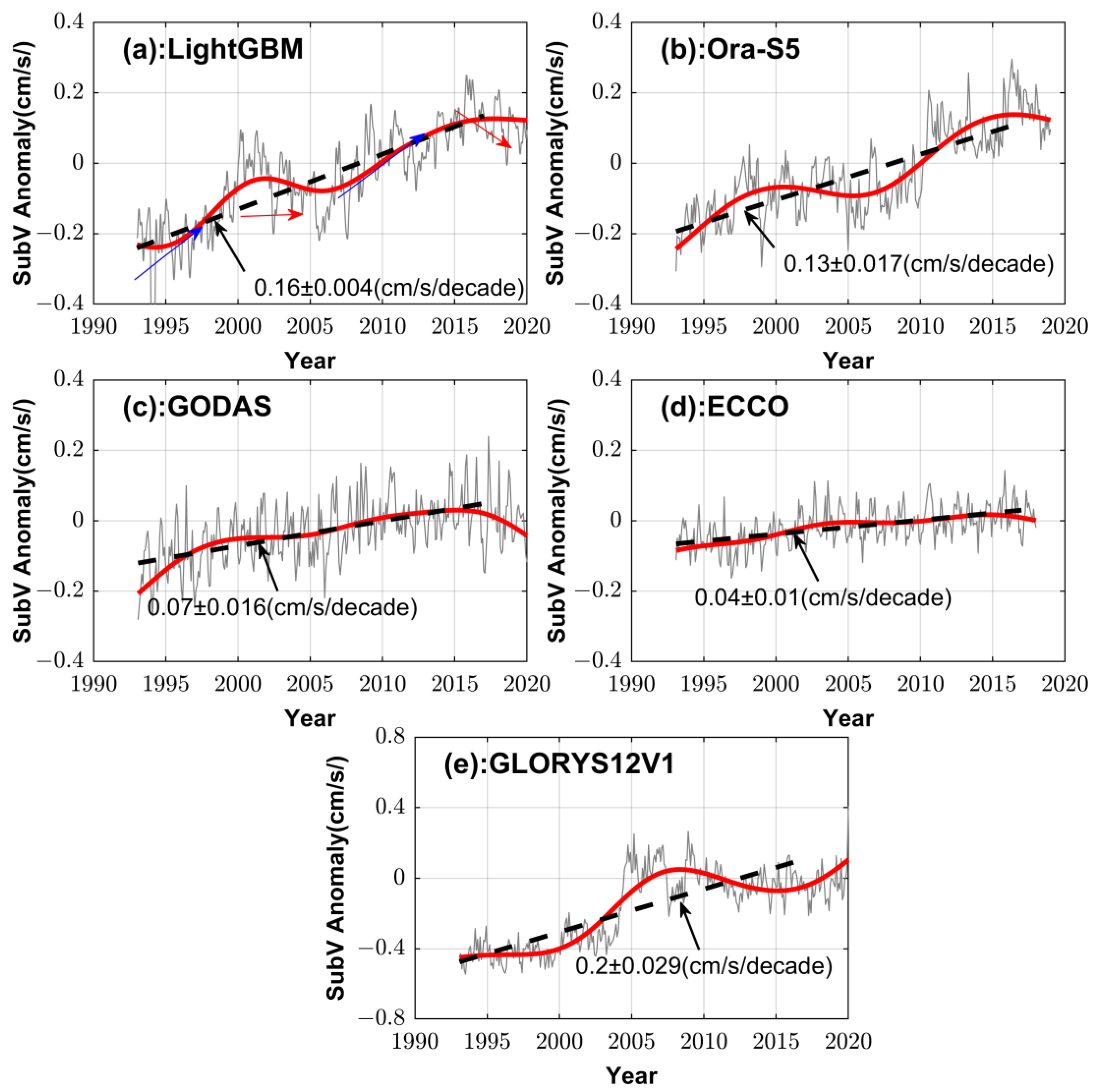
In this section, the variations in average SubV anomaly for LightGBM velocity and the reanalysis datasets (ORA-S5, GODAS, ECCO, and GLORYS12V1) in the SO from 1993 to 2020 were investigated. The LightGBM SubV is retrieved by projecting the surface observations downwards using the LightGBM model (Case 1). Figure 9 shows the spatial average SubV anomaly (grey line) and their 60-month lowpass filtered series (red line) for the five datasets. Here, spatial averaging is performed over the entire study area. In terms of long-term trends, the SubV of the LightGBM SubV has been increasing steadily since 1993. However, there are also variations in the local trend. What is more interesting is that the fluctuations in the local trend cover a period of about 13 years. Within each period, the trend has two phases: an acceleration (indicated by the red arrow) and a slowdown (indicated by the blue arrow). In 2016, the spatial average SubV for the LightGBM datasets attained its highest point. It is evident that the Ora-S5, GODAS, and ECCO SubV anomalies reveal similar variations over the entire study period in the Southern Ocean. Despite differences in localized fluctuations, the GLORYS12V1 SubV has also grown in line with the other four SubVs in terms of long-term trends. And as indicated by the thick black dashed line, all five datasets show a long-term positive trend in the regionally averaged SubV anomalies over the study period, 0.16 ± 0.004 cm/s/decade for the LightGBM, 0.13 ± 0.017 cm/s/decade for ORAS5, 0.074 ± 0.016 cm/s/decade for GODAS, 0.04 ± 0.02 cm/s/decade for ECCO, and 0.20 ± 0.029 cm/s/decade for GLORYS12V1. Due to the smaller velocity magnitude depicted in Figure 6, the trends of the ECCO and GODAS spatial average SubV anomalies are also marginally less than those of other data. Although the trend values for the five SubV anomalies are distinct, their highly consistent growth can be trusted. The positive trend of SubV in the Southern Ocean can be attributed to the effect of the zonal difference of anthropogenic ocean warming and strengthened wind stress [3,4,5]. Strong warming to the north of the Subantarctic Front and moderate warming in the Subantarctic Front, leading to an increase in baroclinicity, accelerate the northern flank of the ACC and adjacent subtropics [4]. Given the high similarity with other reanalysis datasets and earlier research [5], our retrieved SubV is reliable for determining the direction of the Southern Ocean SubV trend. For accurate measurement of the magnitude of the trend for SubV, it remains a challenge for current approaches, whether assimilation methods or machine learning estimation methods are used. Nevertheless, based on the qualitative and quantitative analysis previously conducted in Section 3.2, the higher ability to characterize spatial properties and capture temporal variations of reconstructed subsurface velocities suggests that the trend value of the LightGBM SubV is also more trustworthy than that of the reanalysis SubV datasets. The statistically significant growth trend of the LightGBM SubV provides new evidence for the deep acceleration of the Southern Ocean

4. Conclusions

In this study, we applied the LightGBM model to estimate ocean subsurface velocity at a depth of 1000 dbar in the SO. The sea surface parameters input to the LightGBM model are ADT, SurZV, SurMV, SurZW, and SurMW. The ocean subsurface velocities derived from the Argo trajectory were utilized in the model’s training and validation processes. The sea surface parameters and ocean subsurface velocity used to construct the LightGBM model all come from observational data. The results show that the LightGBM model has a higher accuracy (RMSE = 4.08 cm/s for SubZV and RMSE = 3.97 cm/s for SubMV) than both the RF model and the MLR model. Through quantitative and qualitative evaluation, the subsurface velocities estimated by LightGBM depict the large- and small-scale velocity fields in the Southern Ocean with greater precision than various reanalysis datasets. In particular, the spatial correlation coefficient in 2009 between LightGBM annual SubV and Argo annual SubV reached 0.83. Moreover, the time correlation coefficient of the LightGBM annual SubV is also clearly higher than that of the reanalysis datasets. Since the 1990s, both the SO’s LightGBM and reanalysis velocities at 1000 dbar have increased in the long term, suggesting that our LightGBM model is capable of monitoring large-scale velocity variations in the Southern Ocean.

For the development of a machine learning model, sufficient training data are required. Since the ARGO’s measurements of ocean subsurface velocity are only taken at its parking location, our exploration of the Southern Ocean subsurface velocity estimation using the LightGBM model is limited to a depth of 1000 dbar. Due to the dearth of in situ subsurface velocity measurements, our model is currently inapplicable for estimating subsurface velocity at other depths. Previous studies on 3D velocity field estimation using dynamical methods have shown that the ocean surface observations and the subsurface velocities at other depths are closely related [13,15,19]. With the accumulation of oceanic subsurface velocity observations, the method proposed in this paper for estimating the subsurface velocity field is promising. Care must be taken when estimating the velocity of the upper ocean. Sea surface wind, sea surface temperature, and sea surface salinity deserve to be considered seriously as model inputs because of the strong drive from wind and buoyancy fluxes to the upper ocean circulation [39,40]. Similarly, the topography can be incorporated into the input of ocean velocity estimation models to enhance estimations due to the impact of topographic barriers on ocean circulation [41].

More research is required on this topic. As a continuation of this work, the ability of the estimated subsurface velocity to capture other mesoscale phenomena, such as mesoscale eddies, will be evaluated further. In addition, given the good performance of retrieved subsurface velocities in the Southern Ocean, we also intend to expand our model into the global ocean in order to gain a comprehensive understanding of global ocean subsurface velocities in response to the current global warming. Take note that the vertical density gradient in the SO is comparatively smaller when compared to lower latitudes. This indicates that the SO exhibits a higher degree of barotropic in contrast to regions at lower latitudes. Consequently, the geostrophic currents at the surface are expected to align more closely with those at 1000 m depth. It follows that the performance of the LightGBM model may exhibit variability across different oceanic regions.

References

1. Chen, X.; Tung, K.-K. Global Surface Warming Enhanced by Weak Atlantic Overturning Circulation. Nature 2018, 559, 387–391. [Google Scholar] [CrossRef]
2. Peng, Q.; Xie, S.-P.; Wang, D.; Huang, R.X.; Chen, G.; Shu, Y.; Shi, J.-R.; Liu, W. Surface Warming–Induced Global Acceleration of Upper Ocean Currents. Sci. Adv. 2022, 8, eabj8394. [Google Scholar] [CrossRef] [PubMed]
3. Shi, J.-R.; Talley, L.D.; Xie, S.-P.; Liu, W.; Gille, S.T. Effects of Buoyancy and Wind Forcing on Southern Ocean Climate Change. J. Clim. 2020, 33, 10003–10020. [Google Scholar] [CrossRef]
4. Shi, J.-R.; Talley, L.D.; Xie, S.-P.; Peng, Q.; Liu, W. Ocean Warming and Accelerating Southern Ocean Zonal Flow. Nat. Clim. Chang. 2021, 11, 1090–1097. [Google Scholar] [CrossRef]
5. Hu, S.; Sprintall, J.; Guan, C.; McPhaden, M.J.; Wang, F.; Hu, D.; Cai, W. Deep-Reaching Acceleration of Global Mean Ocean Circulation over the Past Two Decades. Sci. Adv. 2020, 6, eaax7727. [Google Scholar] [CrossRef] [PubMed]
6. Wu, L. Acceleration of Global Mean Ocean Circulation under the Climate Warming. Sci. China Earth Sci. 2020, 63, 1039–1040. [Google Scholar] [CrossRef]
7. Wunsch, C. Is the Ocean Speeding Up? Ocean Surface Energy Trends. J. Phys. Oceanogr. 2020, 50, 3205–3217. [Google Scholar] [CrossRef]
8. Tollefson, J. Sensor Array Provides New Look at Global Ocean Current. Nature 2018, 554, 413–414. [Google Scholar] [CrossRef]
9. Klemas, V.; Yan, X.-H. Subsurface and Deeper Ocean Remote Sensing from Satellites: An Overview and New Results. Prog. Oceanogr. 2014, 122, 1–9. [Google Scholar] [CrossRef]
10. Huang, L.; Zhuang, W.; Wu, Z.; Meng, L.; Edwing, D.; Edwing, K.; Wang, L.; Yan, X. Decadal Cooling Events in the South Indian Ocean during the Argo Era. JGR Ocean. 2022, 127, e2021JC017949. [Google Scholar] [CrossRef]
11. Miao, T.; Huang, H.; Guo, J.; Li, G.; Zhang, Y.; Chen, N. Uncertainty Analysis of Numerical Simulation of Seawater Intrusion Using Deep Learning-Based Surrogate Model. Water 2022, 14, 2933. [Google Scholar] [CrossRef]
12. Morey, S.L.; Gopalakrishnan, G.; Sanz, E.P.; Azevedo Correia De Souza, J.M.; Donohue, K.; Pérez-Brunius, P.; Dukhovskoy, D.; Chassignet, E.; Cornuelle, B.; Bower, A.; et al. Assessment of Numerical Simulations of Deep Circulation and Variability in the Gulf of Mexico Using Recent Observations. J. Phys. Oceanogr. 2020, 50, 1045–1064. [Google Scholar] [CrossRef]
13. Liu, L.; Peng, S.; Huang, R.X. Reconstruction of Ocean’s Interior from Observed Sea Surface Information: Ocean’s interior reconstruction. J. Geophys. Res. Ocean. 2017, 122, 1042–1056. [Google Scholar] [CrossRef]
14. Qiu, B.; Chen, S.; Klein, P.; Torres, H.; Wang, J.; Fu, L.-L.; Menemenlis, D. Reconstructing Upper-Ocean Vertical Velocity Field from Sea Surface Height in the Presence of Unbalanced Motion. J. Phys. Oceanogr. 2020, 50, 55–79. [Google Scholar] [CrossRef]
15. Wang, J.; Flierl, G.R.; LaCasce, J.H.; McClean, J.L.; Mahadevan, A. Reconstructing the Ocean’s Interior from Surface Data. J. Phys. Oceanogr. 2013, 43, 1611–1626. [Google Scholar] [CrossRef]
16. Charantonis, A.A.; Badran, F.; Thiria, S. Retrieving the Evolution of Vertical Profiles of Chlorophyll-a from Satellite Observations Using Hidden Markov Models and Self-Organizing Topological Maps. Remote Sens. Environ. 2015, 163, 229–239. [Google Scholar] [CrossRef]
17. Su, H.; Wu, X.; Yan, X.-H.; Kidwell, A. Estimation of Subsurface Temperature Anomaly in the Indian Ocean during Recent Global Surface Warming Hiatus from Satellite Measurements: A Support Vector Machine Approach. Remote Sens. Environ. 2015, 160, 63–71. [Google Scholar] [CrossRef]
18. LaCasce, J.H.; Mahadevan, A. Estimating Subsurface Horizontal and Vertical Velocities from Sea-Surface Temperature. J. Mar. Res. 2006, 64, 695–721. [Google Scholar] [CrossRef]
19. Liu, L.; Peng, S.; Wang, J.; Huang, R.X. Retrieving Density and Velocity Fields of the Ocean’s Interior from Surface Data. J. Geophys. Res. Ocean. 2014, 119, 8512–8529. [Google Scholar] [CrossRef]
20. Lu, W.; Su, H.; Yang, X.; Yan, X.-H. Subsurface Temperature Estimation from Remote Sensing Data Using a Clustering-Neural Network Method. Remote Sens. Environ. 2019, 229, 213–222. [Google Scholar] [CrossRef]
21. Su, H.; Li, W.; Yan, X.-H. Retrieving Temperature Anomaly in the Global Subsurface and Deeper Ocean From Satellite Observations. J. Geophys. Res. Ocean. 2018, 123, 399–410. [Google Scholar] [CrossRef]
22. Lebedev, K.; Yoshinari, H.; Maximenko, N.; Hacker, P. YoMaHa’07: Velocity Data Assessed from Trajectories of Argo Floats at Parking Level and at the Sea Surface. IPRC Technical Note. 2007. Available online: http://apdrc.soest.hawaii.edu/projects/yomaha/yomaha07/YoMaHa070612.pdf (accessed on 7 December 2023).
23. Talley, L.D.; Feely, R.A.; Sloyan, B.M.; Wanninkhof, R.; Baringer, M.O.; Bullister, J.L.; Carlson, C.A.; Doney, S.C.; Fine, R.A.; Firing, E.; et al. Changes in Ocean Heat, Carbon Content, and Ventilation: A Review of the First Decade of GO-SHIP Global Repeat Hydrography. Annu. Rev. Mar. Sci. 2016, 8, 185–215. [Google Scholar] [CrossRef] [PubMed]
24. Rintoul, S.R. The Global Influence of Localized Dynamics in the Southern Ocean. Nature 2018, 558, 209–218. [Google Scholar] [CrossRef] [PubMed]
25. Armour, K.C.; Marshall, J.; Scott, J.R.; Donohoe, A.; Newsom, E.R. Southern Ocean Warming Delayed by Circumpolar Upwelling and Equatorward Transport. Nat. Geosci 2016, 9, 549–554. [Google Scholar] [CrossRef]
26. Hogg, A.M.C.; Meredith, M.P.; Chambers, D.P.; Abrahamsen, E.P.; Hughes, C.W.; Morrison, A.K. Recent Trends in the Southern Ocean Eddy Field. J. Geophys. Res. Ocean. 2015, 120, 257–267. [Google Scholar] [CrossRef]
27. Bonjean, F.; Lagerloef, G.S.E. Diagnostic Model and Analysis of the Surface Currents in the Tropical Pacific Ocean. J. Phys. Oceanogr. 2002, 32, 2938–2954. [Google Scholar] [CrossRef]
28. Roach, C.J.; Balwada, D.; Speer, K. Global Observations of Horizontal Mixing from Argo Float and Surface Drifter Trajectories. J. Geophys. Res. Ocean. 2018, 123, 4560–4575. [Google Scholar] [CrossRef]
29. Goes, M.; Goni, G.; Dong, S.; Boyer, T.; Baringer, M. The Complementary Value of XBT and Argo Observations to Monitor Ocean Boundary Currents and Meridional Heat and Volume Transports: A Case Study in the Atlantic Ocean. J. Atmos. Ocean. Technol. 2020, 37, 2267–2282. [Google Scholar] [CrossRef]
30. Zanowski, H.; Johnson, G.C.; Lyman, J.M. Equatorial Pacific 1000-dbar Velocity and Isotherm Displacements From Argo Data: Beyond the Mean and Seasonal Cycle. JGR Ocean. 2019, 124, 7873–7882. [Google Scholar] [CrossRef]
31. Ke, G.; Meng, Q.; Finley, T.; Wang, T.; Chen, W.; Ma, W.; Ye, Q.; Liu, T.-Y. LightGBM: A Highly Efficient Gradient Boosting Decision Tree. Adv. Neural Inf. Process. Syst. 2017, 9, 3149–3157. [Google Scholar]
32. Friedman, J.H. Greedy Function Approximation: A Gradient Boosting Machine. Ann. Statist. 2001, 29, 1189–1232. [Google Scholar] [CrossRef]
33. Liaw, A.; Wiener, M. Classification and Regression by randomForest. R News 2002, 2, 18–22. [Google Scholar]
34. Pedregosa, F.; Varoquaux, G.; Gramfort, A.; Michel, V.; Thirion, B.; Grisel, O.; Blondel, M.; Prettenhofer, P.; Weiss, R.; Dubourg, V.; et al. Scikit-Learn: Machine Learning in Python. Mach. Learn. Python 2011, 6, 2825–2830. [Google Scholar]
35. Snoek, J.; Larochelle, H.; Adams, R.P. Practical Bayesian Optimization of Machine Learning Algorithms. Adv. Neural Inf. Process. Syst. 2012, 9. [Google Scholar]
36. Sun, C.; Watts, D.R. A Circumpolar Gravest Empirical Mode for the Southern Ocean Hydrography. J. Geophys. Res. 2001, 106, 2833–2855. [Google Scholar] [CrossRef]
37. Zhang, L.; Sun, C. A Geostrophic Empirical Mode Based on Altimetric Sea Surface Height. Sci. China Earth Sci. 2012, 55, 1193–1205. [Google Scholar] [CrossRef]
38. Chelton, D.B.; Gaube, P.; Schlax, M.G.; Early, J.J.; Samelson, R.M. The Influence of Nonlinear Mesoscale Eddies on Near-Surface Oceanic Chlorophyll. Science 2011, 334, 328–332. [Google Scholar] [CrossRef]
39. Li, H.; Xu, Y. Barotropic and Baroclinic Inverse Kinetic Energy Cascade in the Antarctic Circumpolar Current. J. Phys. Oceanogr. 2021, 51, 809–824. [Google Scholar] [CrossRef]
40. Liu, T.; Ou, H.-W.; Liu, X.; Qian, Y.-K.; Chen, D. The Dependence of Upper Ocean Gyres on Wind and Buoyancy Forcing. Geosci. Lett. 2022, 9, 2. [Google Scholar] [CrossRef]
41. de Boer, A.M.; Hutchinson, D.K.; Roquet, F.; Sime, L.C.; Burls, N.J.; Heuzé, C. The Impact of Southern Ocean Topographic Barriers on the Ocean Circulation and the Overlying Atmosphere. J. Clim. 2022, 35, 5805–5821. [Google Scholar] [CrossRef]
Figure 1. Flowchart for subsurface velocity retrieval in the SO using the LightGBM approach.
Remotesensing 15 05699 g001
Figure 2. The 2D histograms between the reconstructed SubZV (a) and SubMV (b) in Case 1 and the Argo velocity for the validation set. The green dotted lines indicate their fit line. And their fitted equations are shown in the upper left corner, where y represents the parameter in the vertical coordinate and x represents the parameter in the horizontal coordinate. The black dotted lines indicate the equalvalue line.
Remotesensing 15 05699 g002
Figure 3. The 2D histograms between the reconstructed SubZV (a) and SubMV (b) in Case 8 and the Argo velocity for the validation set. The green dotted lines indicate their fit line. And their fitted equations are shown in the upper left corner, where y represents the parameter in the vertical coordinate and x represents the parameter in the horizontal coordinate. The black dotted lines indicate the equalvalue line.
Remotesensing 15 05699 g003
Figure 4. The ocean subsurface velocity strength map for (a) LightGBM (15 January 2009), (b) Ora-S5 (January 2009), (c) GODAS (January 2009), (d) ECCO (15 January 2009), and (e) GLORYS12V1 (15 January 2009) at 1000 dbar in the SO.
Remotesensing 15 05699 g004
Figure 5. The 2D histograms between LightGBM SubV (a), Ora-S5 SubV (b), GODAS SubV (c), ECCO SubV (d), GLORYS12V1 SubV (e), and Argo SubV for the validation set. The green dotted lines indicate their fit line. And their fitted equations are shown in the upper left corner, where y represents the parameter in the vertical coordinate and x represents the parameter in the horizontal coordinate. The black dotted lines indicate the equal-value line.
Remotesensing 15 05699 g005
Figure 6. The annual SubV maps for the Argo (a), LightGBM (b), Ora-S5 (c), GODAS (d), ECCO (e), and GLORYS12V1 (f) in 2009.
Remotesensing 15 05699 g006
Figure 7. The scatter plots between LightGBM (a), Ora-s5 (b), GODAS (c), ECCO (d), GLORYS12V1 (e) annual SubV and Argo annual SubV in 2009. The blue dotted lines indicate their fit line. And their fitted equations are shown in the bottom right corner, where y represents the parameter in the vertical coordinate and x represents the parameter in the horizontal coordinate. The red dotted lines indicate the equal-value line.
Remotesensing 15 05699 g007
Figure 8. The time series of the ARGO (a), LightGBM (b), Ora-S5 (c), GODAS (d), ECCO (e), and GLORYS12V1 (f) monthly SubV at 49.5°S, 127.5°W (marked with the red pentagram in Figure 5a). The blue line denotes the monthly SubV series, and the red line represents the 12-month low-pass filtered series of the monthly SubV. The r in (bf) is the time correlation coefficient between the low-pass filtered series of the LightGBM, Ora-S5, GODAS, ECCO, and GLORYS12V1 and the low-pass filtered series of the ARGO.
Remotesensing 15 05699 g008
Figure 9. Spatial average SubV anomaly curve in the Southern Ocean for LightGBM (a), OraS5 (b), GODAS (c), ECCO (d), and GLORYS12V1 (e) data. The SubV anomaly of all data is obtained by subtracting its multi-year average from 2005 to 2014 (the multi-year average SubV for LightGBM: 6.77 cm/s, Oras5: 5.58 cm/s, GODAS: 2.60 cm/s, ECCO: 2.45 cm/s, GLORYS12V1: 7.63 m/s). The gray lines are the monthly SubV anomaly curves. The red lines are their 60-month low pass-filtered time series. The monthly SubV of LightGBM, GLORYS12V1, and ECCO are the result of 30-day low-pass filtering of their daily SubV. The trends of average SubV for all datasets are denoted in thick black dashed lines.
Remotesensing 15 05699 g009