Detection of Changes in Buildings in Remote Sensing Images via Self-Supervised Contrastive Pre-Training and Historical Geographic Information System Vector Maps

Abstract

The detection of building changes (hereafter ‘building change detection’, BCD) is a critical issue in remote sensing analysis. Accurate BCD faces challenges, such as complex scenes, radiometric differences between bi-temporal images, and a shortage of labelled samples. Traditional supervised deep learning requires abundant labelled data, which is expensive to obtain for BCD. By contrast, there is ample unlabelled remote sensing imagery available. Self-supervised learning (SSL) offers a solution, allowing learning from unlabelled data without explicit labels. Inspired by SSL, we employed the SimSiam algorithm to acquire domain-specific knowledge from remote sensing data. Then, these well-initialised weight parameters were transferred to BCD tasks, achieving optimal accuracy. A novel framework for BCD was developed using self-supervised contrastive pre-training and historical geographic information system (GIS) vector maps (HGVMs). We introduced the improved MS-ResUNet network for the extraction of buildings from new temporal satellite images, incorporating multi-scale pyramid image inputs and multi-layer attention modules. In addition, we pioneered a novel spatial analysis rule for detecting changes in building vectors in bi-temporal images. This rule enabled automatic BCD by harnessing domain knowledge from HGVMs and building upon the spatial analysis of building vectors in bi-temporal images. We applied this method to two extensive datasets in Liuzhou, China, to assess its effectiveness in both urban and suburban areas. The experimental results demonstrated that our proposed approach offers a competitive quantitative and qualitative performance, surpassing existing state-of-the-art methods. Combining HGVMs and high-resolution remote sensing imagery from the corresponding years is useful for building updates.

1. Introduction

China’s rapid urban expansion, driven by the ongoing urbanisation process, is rapidly converting arable land into construction zones to accommodate its burgeoning population [1,2]. However, poorly planned construction projects consume arable land and indirectly contribute to geological disasters. The detection of building changes (hereafter ‘building change detection’, BCD) plays a pivotal role in monitoring urban development and has applications in urban planning, urban expansion, natural disaster assessment, and updating geographic databases [1,2,3,4]. Urban buildings, as fundamental elements of geographic information, have long presented challenges in remote sensing due to their dynamic spatial changes. Buildings are key urban features with diverse forms, and they present unique challenges in high-resolution remote sensing images, where their complexity intensifies with image spatial resolution. Variations in the surface materials, colours, textures, geometry, and other features lead to heightened pixel differences in rooftop areas, influencing BCD results. Furthermore, complex backgrounds and variable building structures in high-resolution images often result in inaccurate recognition. The diversity of building shapes, heights, and their proximity to other features (e.g., trees and roads) further complicates BCD in high-resolution images, giving rise to challenges such as the “same object, different spectra; same spectra, different objects” phenomenon.

With the expansion of geographic information databases and the growing use of crowd-sourced geographic data, open-source vector maps, such as OpenStreetMap, and historical geographic information system (GIS) vector maps (HGVMs) from national surveys have emerged [4,5,6]. These maps provide valuable information for large-scale BCD based on remote sensing imagery, improving the overall accuracy of BCD. However, challenges arise when using HGVMs to assist remote sensing image-based BCD, primarily in geometric registration and building extraction in new temporal images. Data timeliness issues can lead to mismatches between buildings in HGVMs and those in new temporal images. For instance, buildings may disappear in a new temporal image, while their polygons still exist in the HGVM. Conversely, newly added buildings in the new temporal image may not be represented in the HGVM. In summary, current large-scale BCD techniques based on deep learning face several challenges. First, the scarcity of large-scale building datasets hinders the deep learning progress. Acquiring reliable and abundant training samples of buildings, as well as validating the effectiveness of these methods in practical applications, remains essential. Second, traditional end-to-end fully convolutional network models employ pixel-level semantic segmentation strategies, resulting in the loss of building position and edge detail information due to the use of pooling layers. Third, current network models rely solely on image-based building extraction and lack the assistance of GIS vectors, leading to sub-optimal building extraction results. Finally, open-source datasets primarily consist of images from the same sensor or with similar imaging times between the testing and training images. As image resolution increases, preserving the integrity of large building roofs in testing images becomes more difficult, while small buildings are increasingly susceptible to detection omissions. Even after image registration, the influence of variation in building projections can still result in the misalignment of corresponding buildings in temporally distinct heterogeneous images.

In recent years, the leveraging of open-source datasets [7,8,9,10,11,12,13,14,15,16] in the field of BCD research has resulted in a surge of state-of-the-art (SOTA) methods. These methods predominantly rely on deep convolutional neural networks (DCNNs) [17,18,19,20,21,22,23,24] and transformer models [25,26,27,28]. They approach BCD as a high-stakes prediction task, producing pixel-level outputs. However, the scarcity of extensive annotated datasets for BCD, coupled with the inherent complexity of remote sensing imagery, presents considerable challenges in training DCNNs for this specific task. When faced with the challenge of procuring a substantial number of labelled samples, a common recourse has been to transfer the knowledge acquired from the ImageNet dataset to the BCD domain. While ImageNet pre-trained models typically outperform models trained from scratch in tackling BCD problems, their performance remains confined due to the domain disparities between ImageNet and remote sensing images. These inherent distinctions between datasets hinder the efficacy of this transfer learning strategy.

Recently, self-supervised learning (SSL) methods have ushered in a new era in deep learning models [29,30,31,32,33,34,35]. Over the past 2 years, SSL methods have experienced remarkable growth as they endeavour to learn visual representations from vast unlabelled image datasets. Unlike learning methods that rely on precisely annotated samples as guiding signals, SSL methods can extract supervision signals from the abundant pool of unlabelled data, and they excel in feature acquisition. SSL methods capture visual features that exhibit greater distinctiveness and transferability than supervised ImageNet weights [36,37,38,39]. Consequently, they have succeeded in significantly narrowing the gap in representation learning between supervised and unsupervised methods. The most effective SSL methods employ data augmentation techniques to generate positive samples. In essence, they harness data augmentation methods, such as image cropping and rotation, to generate multiple perspectives of the same image. The underlying objective function endeavours to minimise the separation between positive samples in the feature space. For most of these methodologies, a competitive dynamic exists between positive and negative samples. Because these methods do not hinge on the availability of labelled data, they are capable of unsupervised feature learning from an extensive reservoir of unlabelled data, followed by the seamless transfer of weights to other remote sensing tasks. In the absence of labelled samples, SSL methods cultivate a universal visual representation, subsequently fine-tuning it for specific downstream tasks using a limited number of labelled samples. Due to the robust generalisation capabilities of their pre-trained features, these techniques can yield outcomes in specific downstream tasks that rival those achieved by supervised learning models.

Therefore, in this study, we explored the effectiveness of representation learning in the field under both supervised and self-supervised conditions to address the domain differences between remote sensing and the ImageNet dataset. We employed SSL to pre-train domain-specific representations of remote sensing images and transferred the learned features to a downstream BCD dataset. Specifically, we used the SimSiam algorithm to train domain-specific knowledge of remote sensing datasets and then transferred well-initialised weight parameters pre-trained from unlabelled remote sensing imagery to achieve the optimal detection accuracy. We chose the SimSiam algorithm for self-supervised contrastive pre-training due to its simplicity and minimal computational resource requirements. Based on this, we proposed a novel framework for remote sensing image BCD that leveraged self-supervised contrastive pre-training and HGVMs. This framework effectively incorporated semantic information from HGVMs during the BCD process in bi-temporal remote sensing images. In the phase of constructing the building sample library, HGVMs are combined with the corresponding old temporal remote sensing images. The geographical object class information from HGVMs was used to design and create the building sample library. Inspired by Li et al. [24], we proposed an enhanced ResUNet architecture called MS-ResUNet and integrated it with HGVMs for automatic BCD. MS-ResUNet incorporates a multi-scale image pyramid (MIP) structure during the image input phase and uses attention modules to establish connections between the encoder and decoder, enabling the model to capture the abundant feature interactions. MS-ResUnet combines the traditional attention mechanism with linear attention mechanisms (LAMs) to effectively capture global contextual information. In the proposed framework, the SimSiam method is used to pre-train the encoder of the MS-ResUNet model. This encoder has excellent parameter initialisation and can effectively address the downstream task of building extraction from new temporal satellite images. In the BCD phase, we performed a spatial analysis by comparing old temporal building vectors with new temporal building vectors, and we proposed spatial analysis rules for pixel-to-object bi-temporal comparisons. These rules effectively integrate semantic information and boundary constraints from HGVMs and use a majority voting method to preserve the integrity of building change objects. Our primary research contributions are summarised below.

(1)

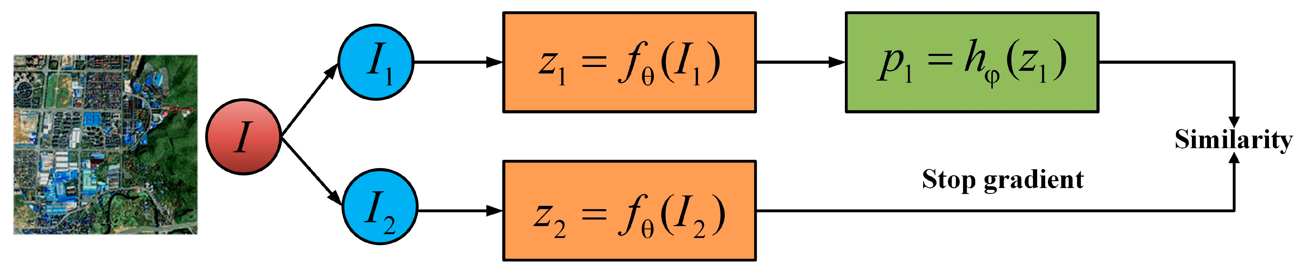
This paper has explored the SimSiam algorithm’s generalisation ability to learn visual representations from remote sensing images. SimSiam leverages unlabelled samples of old temporal building images to acquire effective feature representations when extracting buildings from new temporal imagery. Initially pre-trained by a self-supervised contrastive learning approach, the encoder undergoes fine-tuning, thereby significantly enhancing downstream building extraction networks through well-initialised parameters.

(2)

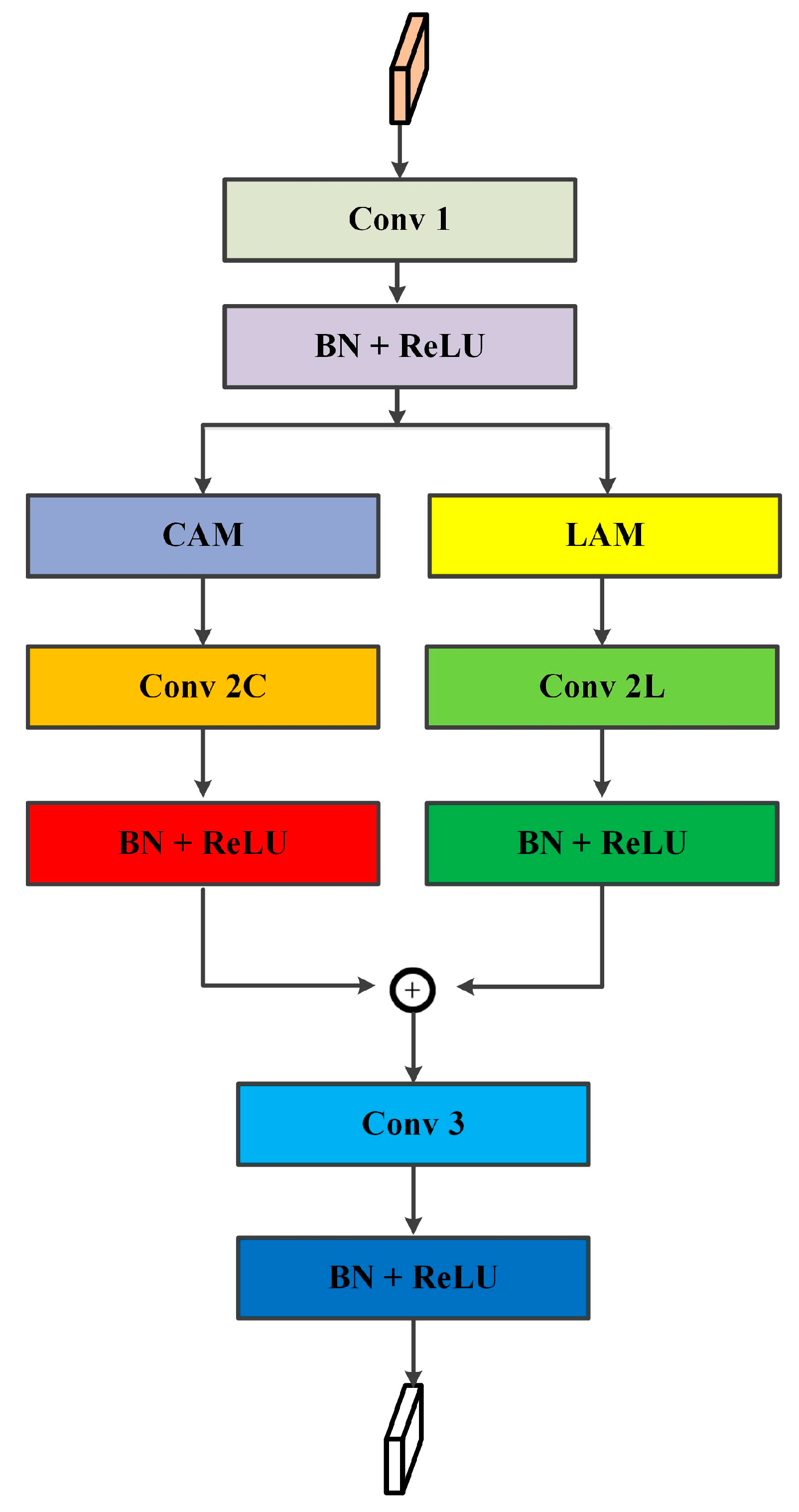
We devised an MS-ResUNet network that incorporates an MIP and multi-layer attention modules, resulting in superior overall accuracy in building extraction compared to SOTA methods.

(3)

We introduced a novel spatial analysis rule to detect changes in building vectors. By leveraging domain knowledge from HGVMs and building upon the spatial analysis of building vectors in bi-temporal images, we achieved an automated BCD.

In the subsequent sections, we review previous studies (Section 2), present our proposed BCD method along with the experimental details (Section 3), present the results of comparisons, and discuss our findings (Section 4). Finally, we present our conclusions in Section 5.

2. Related Work

2.1. Brief Overview of BCD Datasets and Methods

The rise of deep learning has revolutionised BCD by employing DCNNs for end-to-end dense prediction in remote sensing imagery. In high-resolution remote sensing images, deep learning techniques enable the segmentation and labelling of building objects, facilitating the extraction of specific building information. Image semantic segmentation methods merge traditional image segmentation techniques with object recognition, effectively dividing images into distinctive regions with unique characteristics, addressing the issue of precise pixel-level prediction in remote sensing imagery. A range of open-source datasets for building extraction and BCD has emerged, such as the Massachusetts Building Dataset [7], the Inria Aerial Image Labelling Dataset [8], the WHU Aerial Building Dataset [9], the Aerial Imagery for Roof Segmentation (AIRS) [10], LEVIR-CD [11], WHU BCD [12], Google Data Set [13], S2Looking [14], DSIFN [15], and 3DCD [16]. In addition, semantic segmentation methods, predominantly utilising fully convolutional networks (FCNs), have become widely used for building extraction tasks. Noteworthy networks in this field include SegNet [17], UNet [18], UNet++ [19], PSPNet [20], HRNet [21], ResUNet [22], and Deeplab V3+ [23]. The availability of these open-source datasets has significantly accelerated the progress of building extraction and BCD techniques rooted in deep learning.

Currently, within the realm of BCD, a notable supervised technique is the Fully Convolutional Siamese Network (FCSN) [40]. The FCSN typically adopts a dual-branch structure with shared weight parameters and takes bi-temporal remote sensing images as inputs. The network includes specific modules that calculate the similarity between the bi-temporal images. The first FCSN, proposed by Daudt et al. [40], includes three typical structures: FC-EF, FC-Siam-conc, and FC-Siam-diff. These models fuse the differential features and concatenation features of multi-temporal remote sensing images during training to achieve fast and accurate CD maps. Zhang et al. [15] proposed the DSIFN model, which uses the VGG network [41] to extract deep features of bi-temporal remote sensing images and spatial and channel attention modules in the decoder to fuse multi-layer features. Fang et al. [42] proposed the SNUNet model, which is based on the NestedUNet and Siamese networks and uses channel attention modules to enhance image features, solving the issue of position loss of change information in deep networks by employing dense connections. Chen et al. [43] proposed the DASNet model, which mainly utilises attention mechanisms to capture the remote correlation of bi-temporal images and obtain the feature representation of the final change map. Shi et al. [44] proposed the DSAMNet model, which introduces a metric module to learn change features and integrates convolutional block attention modules (CBAMs) to provide more discriminative features. Liu et al. (2021) proposed a super resolution-based CD network (SRCDNet) with a stacked attention module (SAM) to help detect changes and overcome the resolution difference between bi-temporal images. Papadomanolaki et al. [45] proposed the BiDateNet model, which integrates LSTM blocks into the skip connections of UNet to help detect changes between multi-temporal Sentinel-2 data. Song et al. [46] proposed the SUACDNet model, which uses residual structures and three types of attention modules to optimise the network and make it more sensitive to change regions while filtering out background noise. Lee et al. [47] proposed a local similarity Siamese network for handling CD problems in complex urban areas. Subsequently, Yin et al. [48] proposed a unique attention-guided Siamese network (SAGNet) to address the challenges of edge uncertainty and small target omission in the BCD process. Zheng et al. [49] proposed the CLNet model, which uses a special cross-layer block (CLB) to integrate contextual information and multi-scale image features from different stages. The CLB is able to reuse extracted features and capture pixel-level variation in complex scenes. In general, to improve the accuracy of CD, the aforementioned methods emphasise the design of an effective FCSN architecture and adopt common parameter initialisation methods such as random values or ImageNet pre-trained models. However, because there is a lack of prior knowledge in the CD process, the performance of these methods can be limited by the chosen parameter initialisation method, particularly when labelled sample data are insufficient.

2.2. Use of SSL in Remote Sensing CD

SSL methods can acquire universal feature representations that exhibit remarkable generalisation across various downstream tasks [29,30,31,32,33,34,35]. Among these approaches, contrastive learning has recently gained substantial attention in the academic community, demonstrating an impressive performance. Currently, self-supervised learning network models based on pre-training methods fall into three primary categories. The first category encompasses contrastive learning methods, which involve pairing similar samples as positive pairs and dissimilar samples as negative pairs. These models are trained using the InfoNCE loss to maximise the similarity between positive pairs, while increasing the dissimilarity between negative pairs [31]. For example, Chen et al. [50] proposed a self-supervised approach to pixel-level CD in bi-temporal remote sensing images and a self-supervised CD method based on an unlabelled multi-view setting, which can handle multi-temporal remote sensing image data from different sources and times [51]. The second category includes knowledge distillation methods, such as BYOL [34], SimSiam [35], and DINO [52]. These techniques train a student network to predict the representations of a teacher network. In this approach, the teacher network’s weights are updated based on their moving average instead of traditional backpropagation. For example, Yan et al. [53] introduced a novel domain knowledge-guided self-supervised learning method. This method selects high-similarity feature vectors outputted by mean teacher and student networks using cosine similarity, implementing a hard negative sampling strategy that effectively improves CD performance. The third category involves masked image modelling (MIM) methods [54,55], where specific regions of an image are randomly masked, and the model is trained to reconstruct these masked portions. This approach has the advantage of a reduced reliance on large, annotated datasets. By utilising a large number of unlabelled images, it is possible to train highly capable models that can discern and interpret image content. For example, Sun et al. [56] presented RingMo, a foundational model framework for remote sensing that integrates the Patch Incomplete Mask (PIMask) strategy. The framework demonstrated SOTA performance across various tasks, including image classification, object detection, semantic segmentation, and CD.

Self-supervised remote sensing pre-training can learn meaningful feature representations by utilising a large amount of unlabelled remote sensing image data. These meaningful feature representations can improve the performance of various downstream CD tasks, which has drawn the attention of many researchers. Saha et al. [57] proposed a method for multi-sensor CD using only unlabelled target bi-temporal images to train a network involving deep clustering and SSL. Dong et al. [58] proposed a self-supervised representation learning method based on time prediction for CD in remote sensing images. This method transforms bi-temporal images into more consistent feature representations through self-supervision, thereby avoiding semantic supervision or any additional computation. Based on transformed feature representations, the method of Dong et al. obtains better difference images and reduces the propagation error of difference images in CD. Ou et al. [59] used multi-temporal hyperspectral remote sensing images to propose a hyperspectral image CD framework with an SSL pre-trained model. All aforementioned studies apply self-supervised learning directly to downstream small-scale CD datasets to extract seasonally invariant features for unsupervised CD. Similarly, Ramkumar et al. [60,61] proposed a self-supervised pre-training method for natural image scene CD tasks. Jiang et al. [62] proposed a self-supervised global–local contrastive learning (GLCL) framework that extends instance discrimination to pixel-level CD tasks. Through GLCL, features from the same instance with different views are pulled closer together while features from different instances are separated, enhancing the discriminative feature representation from both global and local perspectives for downstream CD tasks. Wang et al. [63] proposed a supervised contrastive pre-training and fine-tuning CD (SCPFCD) framework, which includes two cascading stages: supervised contrastive pre-training and fine-tuning. This SCPFCD framework aims to train a Siamese network for CD tasks based on an encoder with good parameter initialisation. Chen et al. [64] proposed a SaDL method based on contrastive learning, which requires the use of labels and image enhancement to obtain multi-view positive samples used to pre-train the encoder for CD tasks. Compared to other pre-training methods, SaDL achieves the best CD results but requires additional single-temporal images manually labelled by human experts for pre-training, which is extremely expensive.

The approach taken in this study was inspired by the methodologies of previous studies [62,63,64]. It leverages bi-temporal remote sensing images of the study area as positive sample pairs for SSL, effectively eliminating the need for additional data collection during the pre-training phase. Consequently, the BCD framework outlined in this paper adeptly conducts encoder pre-training with limited samples. This pre-trained encoder effectively initialises its parameters, and its features are of substantial value when addressing BCD tasks in high-resolution remote sensing images.

3. Materials and Methods

The holistic workflow of the BCD framework is depicted in Figure 1 and consists of three steps. First, we establish an extraction dataset of buildings utilising historical remote sensing images of the study area in conjunction with the corresponding HGVMs. To this end, we employ the SimSiam algorithm for self-supervised contrastive pre-training using unlabelled historical remote sensing images. Then, we transfer the pre-trained feature weights to downstream tasks, specifically targeting building extraction in new images. Second, after extracting buildings from the images, we introduce an enhanced MS-ResUNet algorithm. This approach integrates MIP features with a multi-level attention ResUNet to amplify the semantic segmentation performance of building extraction. Finally, by amalgamating historical vector maps of buildings and the outcomes of building extraction in new images, we introduce an innovative spatial analysis rule known as pixel-to-object bi-temporal comparison for BCD. Through the integration of HGVMs and the application of self-supervised contrastive pre-training strategies, our proposed methodology offers a robust approach for detecting changes in buildings in bi-temporal remote sensing images, while retaining the semantic information from the HGVMs.

3.1. Self-Supervised Contrastive Pre-Training Using SimSiam

Due to the high cost of annotating sample labels in remote sensing images and the availability of a large number of unlabelled remote sensing images, self-supervised contrastive pre-training methods have received significant attention in recent years. Features learned through self-supervised contrastive pre-training algorithms generally exhibit an excellent generalisation performance. However, these methods have a major drawback in that they demand substantial computational resources. This is primarily driven by the three factors of negative samples, large batch sizes, and momentum encoders. In contrast to other self-supervised contrastive pre-training methods, the SimSiam algorithm eliminates the need for any of the aforementioned factors, which makes it highly computationally efficient. Therefore, in this study, we employ the SimSiam algorithm to learn the visual features of remote sensing images. The schematic diagram of this algorithm is depicted in Figure 2. Our methodology consists of two main steps. First, we use the SimSiam algorithm for self-supervised pre-training, and then, the pre-trained feature weights obtained in the first step are transferred to downstream building extraction tasks and that extraction network is fine-tuned to enhance the performance of segmentation.

In this study, the image I was subjected to data augmentation, resulting in two distinct perspectives, I₁ and I₂. Both were fed into the two sides of the Siamese neural network (SNN) architecture and processed using the encoder f. The encoder utilised a ResNet50 backbone network and an MLP projection head to extract features from the input images, transforming them from the pixel space into a smaller feature space. The projection head in the encoder f included three MLP layers, each with batch normalisation, including the output layer. Next, the prediction head MLP(h) merged the output of the encoder from perspective I₁ and matched its dimension with the encoder output at the bottom of the architecture. At this point, the MLP(h) consisted of two fully connected layers and a hidden layer with batch normalisation applied. The trained weights were shared on both sides of the model.

To address the high computational resource requirement, the SimSiam approach employs a stop-gradient operator on one side of the architecture. When the stop-gradient operator is applied to either side of the network, the gradients on that side are not updated through backpropagation. The proposed cost function is straightforward and is defined as the cosine similarity function between two vectors. Representing the output vectors of the two perspectives as $p_1\triangleq h\left(f\left(I_1\right)\right)$ and $z_2\triangleq f\left(I_2\right)$, where $h\left(f\left(I_1\right)\right)$ represents the output of the prediction head applied to $f\left(I_1\right)$, and $f\left(·\right)$ is the backbone network applied to both perspectives, the objective function can be defined as follows:

$$D\left(p_1,z_2\right)=-\frac{p_1}{{‖p_1‖}_2}·\frac{z_2}{{‖z_2‖}_2}$$

(1)

In the above equation, $‖·‖$ represents the $L_2$ norm. The final cost function is a symmetric function defined as follows:

$$L=\frac{1}{2}D\left(p_1,z_2\right)+\frac{1}{2}D\left(p_2,z_1\right),p_2\triangleq h\left(f\left(I_2\right)\right)$$

(2)

The cost of all images in the batch is averaged, resulting in the total loss. A critical component that ensures the effectiveness of this algorithm is the stop gradient operator. This operator is applied to the features extracted from each view. As a result, the final cost function is defined as follows:

$$L=\frac{1}{2}D\left(p_1,\mathrm{stopgrad}\left(z_2\right)\right)+\frac{1}{2}D\left(p_2,\mathrm{stopgrad}\left(z_1\right)\right)$$

(3)

This relationship signifies that the defined cost function is entirely symmetric. In addition, when the corresponding views are fed into the network from the top of the architecture, only the gradients are updated.

3.2. New Temporal Building Extraction Based on MS-ResUNet

This study introduces an enhanced MS-ResUNet designed for building extraction from new temporal satellite images, as shown in Figure 3. The architecture incorporates an MIP structure during the image input phase. This allows the network to learn image features across various scales and perform multi-scale feature fusion, thereby enhancing the effective propagation of feature information throughout the model. The architecture follows a sequential model approach, encompassing sequential layers that include an input layer with a pyramid structure, encoder layers, decoder layers, attention layers, and output layers. In contrast to the conventional U-Net design, where basic skip connections simply concatenate shallow and high-level features without intricate processing, MS-ResUNet employs attention modules to establish connections between the encoder and decoder. This departure from traditional skip connections enables the model to capture more feature interactions. To facilitate this, ResNet50 is adopted as the foundational architecture, allowing the attention modules to effectively integrate shallow and high-level features, thereby refining the network’s capacity to capture multi-scale feature representations. To optimise the computational efficiency, the attention module structure, depicted in Figure 4, combines a classical attention mechanism with LAMs to capture comprehensive contextual information. This hybrid approach enables the effective acquisition of global contextual cues. The network’s loss function adheres to the following formula:

$$Loss=-\frac{1}{M}{\displaystyle \sum _{c=1}^C{\displaystyle \sum _{m=1}^M{w}_c·y_m^c·log\left(h_{\mathsf{\theta }}\left(x_m,c\right)\right)}}$$

(4)

where $M$ represents the total number of training samples, $C$ is the count of classes, $y_m^c$ is the target label for training period $m$ of class $c$, $w_c$ denotes the weight assigned to class $c$, $x_m$ is the input of training example $m$, and $h_{\mathsf{\theta }}$ refers to the model endowed with weights $\mathsf{\theta }$.

For the attention module LAM, it is assumed that the length of the input image data is N, the number of input image data channels is C, and the height and width of the input image are H and W, where $N=H\times W$. The input feature data are $X=\left[x_1,\cdots ,x_N\right]\in {ℝ}^{N\times C}$. The dot-product attention mechanism uses three projection matrices, namely, $W_q\in {ℝ}^{D_x\times D_q}$, $W_k\in {ℝ}^{D_x\times D_k}$, and $W_v\in {ℝ}^{D_x\times D_v}$, to generate the corresponding query matrix $Q$, key matrix $K$, and value matrix $V$. According to [24], the attention mechanism is calculated as follows:

$$D\left(Q,K,V\right)=\mathrm{softmax}\left(\frac{Q{K}^T}{\sqrt{d_k}}\right)V$$

(5)

where $d_k$ is a scaling factor. Because $Q\in {ℝ}^{N\times D_k}$ and $K^T\in {ℝ}^{D_k\times N}$, the product of $Q$ and $K^T$ belongs to ${ℝ}^{N\times N}$, resulting in $O\left(N_2\right)$ memory and computational complexity. Therefore, the $i_{th}$ row of the result matrix generated by the dot-product attention module can be represented as follows:

$$D{\left(Q,K,V\right)}_i=\frac{{\displaystyle \sum _{j=1}^N{e}^{q_i^T{k}_j}}{v}_j}{{\displaystyle \sum _{j=1}^N{e}^{q_i^T{k}_j}}}$$

(6)

We generalise Equation (6), then approximate $e^{q_i^T{k}_j}$ using a first-order Taylor expansion, and finally L2-normalise the resulting equation. Equation (6) can be further expressed as follows:

$$D\left(Q,K,V\right)=\frac{{\displaystyle \sum _j{V}_{i,j}}+{\left(\frac{Q}{{‖Q‖}_2}\right)}^T\left({\left(\frac{K}{{‖K‖}_2}\right)}^{T}V\right)}{N+\left(\frac{Q}{{‖Q‖}_2}\right){\displaystyle \sum _j{\left(\frac{K}{{‖K‖}_2}\right)}_{i,j}^T}}$$

(7)

Because ${\displaystyle \sum _{j=1}^N\left(\left(k_j\right)/\left({‖k_j‖}_2\right)\right)}{v}_j^T$ and ${\displaystyle \sum _{j=1}^N\left(\left(k_j\right)/\left({‖k_j‖}_2\right)\right)}$ are shared for every query, the complexity of the LAM is $O\left(N\right)$. However, for channel-wise dot-product attention, considering that the number of channels C in the input is much smaller than the number of pixels, MS-ResUNet combines low-level and high-level feature maps in multiple stages through attention blocks, using ResNet50 as the backbone network.

3.3. BCD Based on A Spatial Analysis

Buildings from bi-temporal remote sensing images are used as the analytical units for BCD. Specifically, for buildings (B1) in the T1 temporal image, the corresponding buildings (B2) are identified in the T2 temporal image, and the spatial overlap between B1 and B2 is recorded. If the overlap between B1 and B2, expressed as the intersection-to-union (IoU) ratio, exceeds a pre-determined threshold (set at 0.5 in this study), the two entities are categorised as “unchanged.” Conversely, if the overlap falls below this threshold, they are classified as “changed.” For illustration, in Figure 5, a and d represent the same building and were categorised as “unchanged” due to their substantial overlap. Conversely, buildings c and f exhibited no spatial overlap and were therefore classified as “changed.” In addition, buildings b and e corresponded spatially but with a relatively modest overlap, necessitating a pixel-level comparison to identify the changed building region denoted as g.

Variations in building projections may lead to positional discrepancies in corresponding structures. Despite advances in image registration accuracy, achieving absolute registration remains challenging. High-rise buildings in registered images may still exhibit positional deviations. To address this issue, the BCD process depicted in Figure 6 was developed. This process has three primary stages, summarised below.

(1)

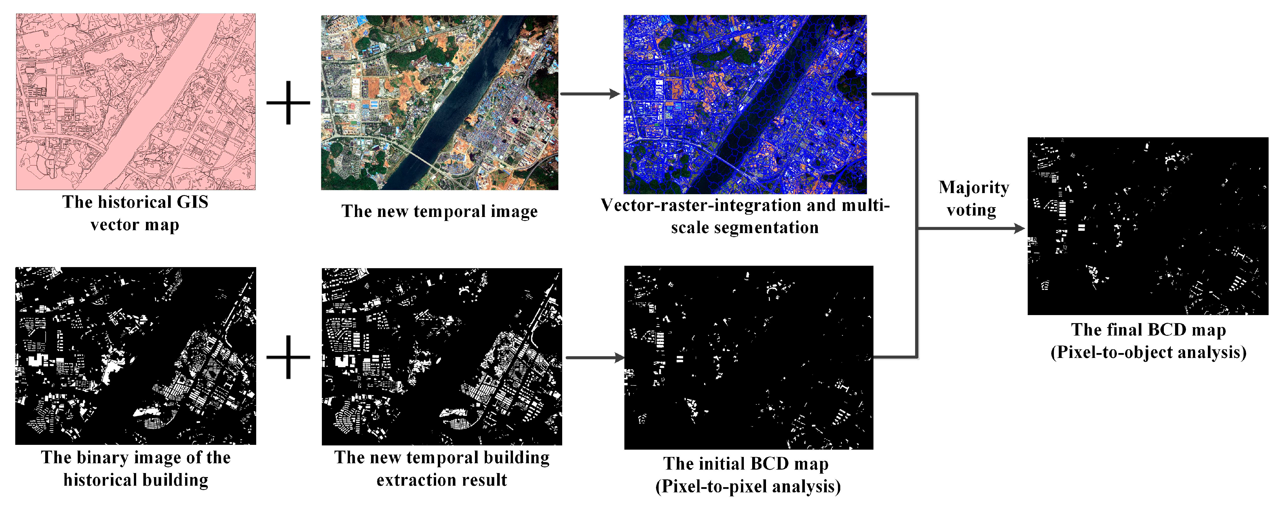
The T2 temporal remote sensing images are overlaid with HGVMs through raster–vector integration. This is followed by meticulous segmentation within vector boundaries, bolstering the building boundary and rooftop integrity using GIS vector constraints to yield segmented objects of varying scales. In this study, we utilised the Estimation of Scale Parameter tool (a plug-in based on the eCognition software 8.7 [65]) for optimal segmentation.

(2)

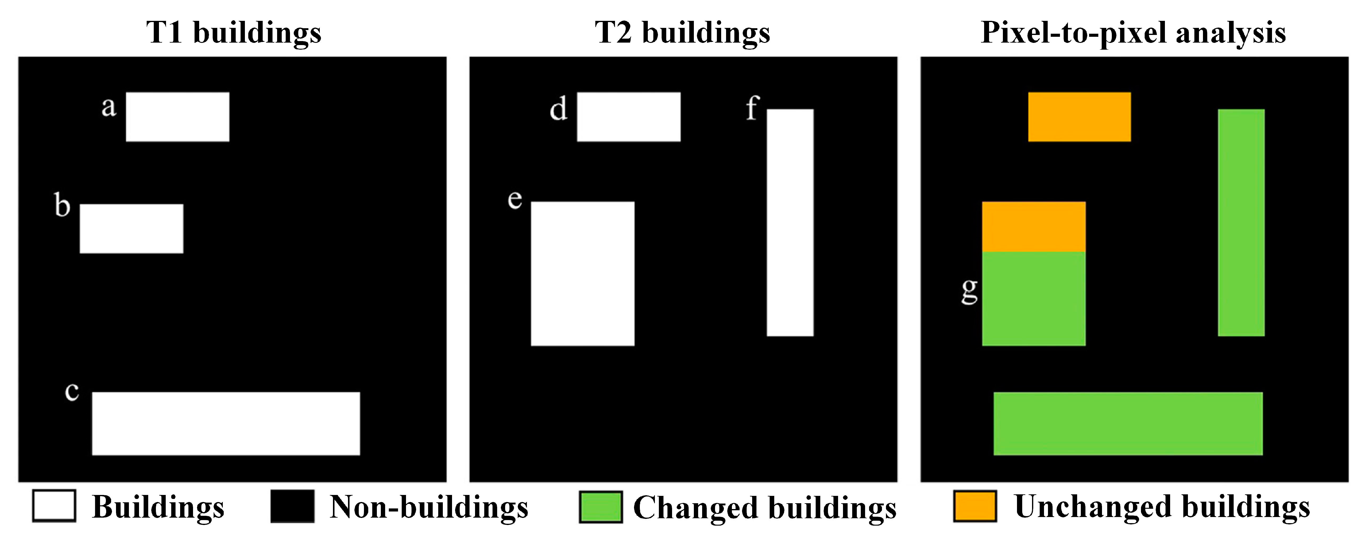
Following the extraction of buildings from the T2 temporal image, spatial analysis is conducted following the pixel-to-pixel comparison rules shown in Figure 5 to determine BCD between the T1 and T2 temporal image buildings.

(3)

To further preserve the integrity of changed building objects, a majority voting strategy is employed to achieve the final BCD and building extraction outcome.

3.4. Experimental Datasets

We collected 19 sets of 2015 GaoFen-2 (GF-2) and WorldView-2 (WV-2) satellite images covering Liuzhou City, China, along with corresponding GIS vector maps. Using the information from these vector maps, we extracted building footprints and converted them into pixel-level annotations through rasterisation. Both raster and vector data were sourced from China’s national geographic census data. The HGVMs, meticulously crafted by survey department experts using high-resolution remote sensing images from the relevant year at a scale of 1:10,000, blend field surveys and manual annotations to generate vector outlines meeting the criteria of China’s national geographic census. These images underwent pre-processing (i.e., data fusion and orthorectification), resulting in fused GF-2 images at 0.8 m resolution and fused WV-2 images at 0.5 m resolution. The images were composed of red, green, and blue channels. All of the WV-2 images were resampled to match the 0.8 m resolution. The data are shown in Figure 7. These images ranged in size from 3000 × 3000 to 10,000 × 10,000 pixels, covering a total area of 237.42 km². The 19 old temporal images were divided into non-overlapping 256 × 256-pixel blocks, excluding samples without building content. This resulted in a dataset of more than 55,000 image samples and their corresponding annotated blocks. We used these samples for network training and performed building extraction on the new temporal images.

During self-supervised contrastive pre-training using the SimSiam algorithm, we exclusively used these remote sensing image blocks and did not use the corresponding labelled blocks. The data augmentation process included random cropping, resizing, random horizontal or vertical flips, and colour transformations applied to the 256 × 256-pixel remote sensing image blocks, generating positive and negative view pairs from these unlabelled image blocks. Then, these pairs were input into the encoder network section of the SimSiam algorithm. The encoder aided the extraction of the image representations of these view pairs, with the final cost function aiming to minimise the difference between similar representations and maximise the difference between dissimilar ones. Finally, the pre-trained encoder was fine-tuned, effectively enhancing the downstream building extraction network for new temporal images by leveraging favourable parameter initialisation.

To validate the effectiveness of our proposed method, we conducted experiments using two large-scale, bi-temporal remote sensing image datasets. Both datasets were situated in Liuzhou City and were also sourced from national geographic survey data. In each dataset, the regions of interest for BCD encompassed urban and rural areas with a concentration of residential structures. These areas had consistent building density patterns, organised layouts, and comparable structural characteristics. The datasets also encompassed independent housing structures, including large-scale urban buildings and scattered residential units. In Experiment Dataset 1 (DS1), the old temporal GF-2 image (Figure 8a) was captured in April 2015, while the new temporal WV-2 image (Figure 8b) was taken in May 2017. The images were sized at 5748 × 4252 pixels. Corresponding to the old temporal GF-2 image, the HGVM (Figure 8c) depicted the area’s 2015 land cover and included 1776 building roof objects. The building change vector data included 848 change objects. The binary building change map (Figure 8d) was generated through vector-to-raster conversion. This dataset represented a typical urban scene with diverse building variation.

In Experiment Dataset 2 (DS2), the old temporal GF-2 image (Figure 9a) was captured in June 2015, and the new temporal WV-2 image (Figure 9b) was taken in November 2017. The images were sized at 4946 × 3674 pixels. The HGVM (Figure 9c) included 1582 building roof objects. The building change vector data included 792 change objects. The binary building change map is shown in Figure 9d. This dataset represented an urban area with varying building distributions, sizes, and structures, including temporary and unauthorised constructions, demolitions, and incomplete construction sites.

3.5. Implementation Details and Evaluation Metrics

We implemented the algorithm proposed in this paper using the PyTorch framework and conducted experiments on a workstation equipped with a 12th Gen Intel Core i9-12900K @ 3.19 GHz processor, a 64 GB RAM, and a NVIDIA GeForce RTX 3090 graphics card. The SimSiam algorithm’s encoder consisted of a backbone network, a projection head, and a prediction head. ResNet50 served as the backbone network. During the SimSiam pre-training phase, we used a stochastic gradient descent (SGD) optimiser with a batch size of 50 and a base learning rate of 0.05. The learning rate followed a cosine decay schedule [31]. We set the weight decay to 0.0001 and the SGD momentum to 0.9 and trained for 400 epochs. We evaluated the performance of the SimSiam algorithm on the downstream tasks of building extraction and CD through fine-tuning. For consistency, we used ResNet50 as the feature extractor during fine-tuning and employed the improved MS-ResUNet model. During the fine-tuning stage of MS-ResUNet, we did not apply data augmentation to the input data. The best performance of MS-ResUNet was achieved with the following configuration: we used the AdamW optimiser with an initial learning rate of 0.003 and batch size of 64 and trained for 150 epochs with early stopping expected after 20 epochs of patience. In this stage, we also applied the cosine decay schedule. We compared the performance of our algorithm to SOTA methods using four metrics: precision, recall, F1 score, and IoU. These metrics were defined as follows:

$$precision=\frac{TP}{TP+FP}$$

(8)

$$recall=\frac{TP}{TP+FN}$$

(9)

$$F1=\frac{2\times precision\times recall}{precision+recall}$$

(10)

$$IoU=\frac{TP}{TP+FP+FN}$$

(11)

where TP, TN, FP, and FN denote true-positive, true-negative, false-positive, and false-negative values, respectively.

3.6. Comparison with SOTA Approaches

We compared our proposed MS-ResUNet method for BCD with several SOTA approaches, including UNet++ [19], ResUNet [22], PSPNet [20], DeeplabV3+ [23], and HRNet [21]. PSPNet utilises a pyramid pooling module to aggregate contextual information from different regions of images, enabling the incorporation of complex contextual information into a pixel-level semantic segmentation framework. UNet++ and ResUNet are both improvements upon the traditional UNet architecture. UNet++ inherits UNet’s structure while also having the features of DenseNet’s dense connectivity [66], which maximises the preservation of both fine-grained details and global information. Alternatively, ResUNet combines the advantages of residual networks and UNet. DeeplabV3+ employs atrous spatial pyramid pooling (ASPP) [23] to capture multi-scale contextual information from images and introduces a new decoder module to further integrate low-level and high-level feature information. HRNet changes the link between high-resolution and low-resolution feature maps from a serial connection to a parallel one, thus maintaining high-resolution feature map representations throughout the entire network structure. To evaluate the effectiveness of the proposed pre-training method, we conducted a detailed comparative analysis with several other self-supervised pre-training approaches, namely, SimCLR [31], CMC [29], BT [33], MoCo v2 [30], and BYOL [34].

4. Experimental Analyses and Discussion

4.1. Performance Comparison for DS1

4.1.1. Comparison with SOTA Methods

The BCD results for DS1 using different SOTA methods are presented in Figure 10. To provide a more detailed comparison of the results among the different SOTA methods, Figure 11 displays the BCD outcomes for four scenarios featuring various building scenes. From left to right, these scenarios include the old temporal image from 2015, the new temporal image from 2017, the ground truth, and the results of UNet++, ResUNet, PSPNet, DeeplabV3+, HRNet, and MS-ResUNet. In DS1, the industrial area is primarily made up of low-rise buildings, with the rooftops of factory buildings distributed unevenly and varying in size. The residential areas include many newly constructed and demolished buildings. As construction projects are completed, some of the temporary low-rise shed-like structures disappear. In each community, the distribution of building rooftops is uniform, and the spectral characteristics are similar. The different residential rooftops exhibit significant differences in size and height. Within the DS1 images, there are both low-rise buildings with minimal projection differences and high-rise buildings with substantial projection differences, and these rooftops exhibit pronounced heterogeneity. From these detailed images, it is clear that the experimental areas selected for this study were highly representative and presented considerable challenges.

During the BCD process, multi-scale segmentation was conducted on the new temporal images from DS1, guided by an HGVM. The chosen scale range spanned from 10 to 100 in increments of 10. The colour weight factor was set to 0.7, the shape weight factor was set to 0.3, and both the smoothness and compactness weight factors were fixed at 0.5. The segmentation results at a scale of 40 were visually selected for post-processing in BCD, using a majority voting strategy to ensure object homogeneity.

Table 1. Comparison of the performance of different SOTA methods for DS1.

Type	Methods	ImageNet Pre-Training	DS1
			Precision	Recall	F1	IoU
Supervised method	UNet++	✔	77.97	86.42	81.98	69.46
	ResUNet	✔	78.04	87.81	82.64	70.42
	PSPNet	✔	74.74	86.40	80.15	66.87
	DeeplabV3+	✔	79.86	87.95	83.71	71.98
	HRNet	✔	80.83	87.33	83.96	72.35
	MS-ResUNet	✔	83.16	89.75	86.32	75.94

Developed as part of the present study. All values are percentages. Bold text indicates the highest values. ✔ indicates the inclusion of this step in the training process.

presents the precision evaluation results of different SOTA methods for BCD. Using these SOTA methods, we incorporated ImageNet pre-trained weights during the model training process. The outcomes clearly demonstrate that the MS-ResUNet method proposed in this study significantly enhanced the quality of BCD. Among all of the model comparisons, MS-ResUNet achieved the highest performance with an F1 score of 86.32% and an IoU score of 75.94%. As shown by the BCD results depicted in Figure 10i, they were closely aligned with the ground truth (Figure 10c). These findings firmly establish that the proposed approach is exceptionally well suited for BCD.

4.1.2. Comparison with Recent SSL Methods

In our downstream BCD tasks, we opted not to employ transformer models with global self-attention mechanisms. Instead, we used an enhanced MS-ResUNet network to address BCD at various scales. We incorporated the efficient ResNet 50 in the encoder and employed an MIP for input. Between the encoder and decoder, we integrated multi-level attention modules to facilitate feature interactions. This departure from traditional skip connections enabled the model to capture more feature interactions and generate more accurate building feature maps. Comparative experiments demonstrated that our MS-ResUNet outperformed other SOTA models, which makes it better suited for downstream tasks. To assess the effectiveness of different self-supervised contrastive pre-training methods, we fine-tuned our MS-ResUNet network using parameters from SimCLR, CMC, BT, MoCo v2, BYOL, and SimSiam. For a fair comparison, we initialised only the backbone part of the MS-ResUNet network, i.e., the ResNet 50 encoder, with pre-trained model parameters. The results for DS2 are shown in Figure 12, while Figure 13 shows the BCD results in various building scene scenarios. As summarised in

Table 2. Performance of the MS-ResUNet model for DS1 using different self-supervised contrastive pre-training methods.

Type	Methods	SSL Pre-Training	DS1
			Precision	Recall	F1	IoU
Self-supervised method	SimCLR	✔	83.26	89.73	86.38	76.02
	CMC	✔	83.94	90.21	86.96	76.93
	BT	✔	84.64	89.85	87.16	77.25
	MoCo v2	✔	84.59	90.54	87.46	77.72
	BYOL	✔	84.84	90.39	87.53	77.82
	SimSiam	✔	85.59	91.26	88.34	79.11

Developed as part of the present study. All values are percentages. Bold text indicates the highest values. ✔ indicates the inclusion of this step in the training process.

, our use of the SimSiam pre-training method achieved the highest F1 score (88.34%) and IoU score (79.11%). BYOL and MoCo v2 attained the second and third highest F1 scores (87.53% and 87.46%, respectively), along with IoU scores of 77.82% and 77.72%, respectively. These scores surpassed the accuracy of models pre-trained on ImageNet (F1: 86.32%, IoU: 75.94%). This underscores the ability of auxiliary tasks in self-supervised contrastive pre-training to capture additional discriminative features from unlabelled data, which, when transferred to downstream networks, significantly enhanced the downstream task performance.

4.2. Performance Comparison for DS2

4.2.1. Comparison with SOTA Methods

The BCD results using different SOTA methods for DS2 are shown in Figure 14. A more detailed comparison of the results among different SOTA methods is presented in Figure 15. Several observations can be made. In the industrial area, low-rise buildings dominate, although their distribution is uneven. The rooftops of these buildings vary in size and structure, with some temporary makeshift roofs used for construction projects. The old temporal imagery from 2015 and the new temporal imagery from 2017 exhibit minimal differences in building projections, and the rooftops display strong homogeneity. In the residential community areas, as construction projects are completed, some temporary makeshift roofs disappear. These areas contain both newly constructed and demolished buildings. Sub-region A includes both low-rise buildings with minimal projection differences and high-rise buildings with significant projection differences. While the rooftops of these buildings exhibit heterogeneity, the geometric displacement between adjacent building rooftops remains relatively consistent. Sub-region B contains a significant number of low-rise tile-roofed houses that were demolished, together with a few newly constructed rooftops. Sub-regions C and D contain a large number of newly constructed houses with dense and complex rooftops. These rooftops vary in size, structure, and distribution, and their homogeneity is relatively low.

In DS2, a scale range from 10 to 100 was maintained with increments of 10. The colour weight was set to 0.7, the shape weight was set to 0.3, and both smoothness and compactness weights were set to 0.5. Segmentation at a scale of 60 was chosen through visual interpretation for a spatial analysis of BCD, ensuring the completeness of building change objects.

Table 3. Comparison of the performance of different SOTA methods on DS2.

Type	Methods	ImageNet Pre-Training	DS2
			Precision	Recall	F1	IoU
Supervised method	UNet++	✔	75.27	85.29	79.97	66.62
	ResUNet	✔	75.87	85.55	80.42	67.25
	PSPNet	✔	73.49	85.28	78.95	65.22
	DeeplabV3+	✔	76.89	85.83	81.11	68.22
	HRNet	✔	77.27	87.45	82.20	69.34
	MS-ResUNet	✔	80.03	87.49	83.59	71.81

Developed as part of the present study. All values are percentages. Bold text indicates the highest values. ✔ indicates the inclusion of this step in the training process.

provides the precision evaluation results for the different SOTA methods in BCD. Using these SOTA methods, we employed ImageNet pre-trained weights during model training. The proposed method significantly enhanced the quality of BCD. Of all models, it achieved the best performance (F1, 83.59%; IoU, 71.81%). As seen in Figure 14i, it was closely aligned with the ground truth shown in Figure 14c. Compared to the SOTA methods, the spatial analysis rules applied in this study were more adaptable to BCD tasks from heterogeneous sensors and were suitable for large-scale BCD across extensive geographic areas.

4.2.2. Comparison with Recent SSL Methods

In DS2, to assess the effectiveness of various self-supervised contrastive pre-training methods, we fine-tuned the downstream MS-ResUNet network using the encoder parameters pre-trained from SimCLR, CMC, BT, MoCo v2, BYOL, and SimSiam. The quantitative visual comparison results for DS2 are shown in Figure 16. Figure 17 displays BCD results featuring different area scenes. As summarised in

Table 4. Performance of the MS-ResUNet model for DS2 using different self-supervised contrastive pre-training methods.

Type	Methods	SSL Pre-Training	DS2
			Precision	Recall	F1	IoU
Self-supervised method	SimCLR	✔	80.35	87.34	83.70	71.96
	CMC	✔	79.92	87.50	83.54	71.73
	BT	✔	80.44	88.17	84.13	72.61
	MoCo v2	✔	80.50	87.79	83.99	72.40
	BYOL	✔	80.37	88.15	84.08	72.53
	SimSiam	✔	80.75	88.54	84.47	73.11

Developed as part of the present study. All values are percentages. Bold text indicates the highest values. ✔ indicates the inclusion of this step in the training process.

, our adoption of the SimSiam pre-training method achieved the highest F1 score (84.47%) and IoU score (73.11%). BT and BYOL obtained the second and third highest F1 scores (84.13% and 84.08%, respectively), along with IoU scores of 72.61% and 72.53%, respectively. These scores outperformed the accuracy (F1: 83.59%, IoU: 71.81%) of ImageNet pre-training, which relies on a large sample size. This confirms that self-supervised contrastive pre-training methods can effectively capture valuable discriminative features from unlabelled image samples and transfer prior knowledge from unlabelled samples to downstream networks to enhance detection accuracy.

4.3. Discussion

4.3.1. Ablation Experiment

Most current architectural frameworks for building extraction rely on encoder–decoder structures. However, they often lack the necessary feature discrimination capabilities to effectively distinguish between small and similar contextual scenes. We therefore conducted a thorough analysis of the individual modules within the MS-ResUNet framework proposed in this paper and their influence on the performance of building extraction and CD. After pre-training with self-supervised contrastive learning using SimSiam, we delved deeper into the MIP module and the attention block module. Our aim was to enhance the model’s ability to maintain building consistency and capture fine details. The experimental results provide compelling evidence that the approach surpasses other SOTA methods based on two extensive building test datasets. To comprehensively evaluate the contributions of the MIP module and the attention block module, we conducted a series of ablation studies on these two dataset groups (

Table 5. Results of an ablation study on the MIP and the attention block module dataset groups.

Model	SimSiam Pre-Training	DS1		DS2
		F1	IoU	F1	IoU
MS-ResUNet without MIP	✔	85.45	76.87	80.84	68.92
MS-ResUNet without attention block	✔	86.67	77.15	81.93	70.95
MS-ResUNet	✔	88.34	79.11	84.47	73.11

Developed as part of the present study. All values are percentages. Bold text indicates the highest values. ✔ indicates the inclusion of this step in the training process.

). In the absence of the attention block module, it achieved an F1 score of 86.67% and an IoU score of 77.15% for DS1, and an F1 score of 81.93% and an IoU score of 70.95% for DS2. Similarly, without the MIP module, it still performed impressively, achieving an F1 score of 85.45% and an IoU score of 76.87% for DS1, and an F1 score of 80.84% and an IoU score of 68.92% for DS2. However, when the MIP module was combined with the attention block module, it delivered exceptional results, achieving an F1 score of 88.34% and an IoU score of 79.11% for DS1, and an F1 score of 84.47% and an IoU score of 73.11% for DS2. This performance clearly surpasses those of previous methods and further confirms the efficacy of our model.

4.3.2. Efficiency under Limited Labels

For large-scale BCD tasks, there is currently a lack of sufficiently large and publicly available annotated datasets. This hinders the further use of deep learning on remote sensing data. Annotating regions of change in bi-temporal remote sensing images from large-scale datasets is an expensive, cumbersome, time-consuming, and mainly manual process. There is an urgent need to develop methods that can learn and represent visual information in images without the need for annotated samples. Therefore, to thoroughly validate the performance of our model using a small number of annotated samples, we compared the impact of ImageNet pre-training methods and various self-supervised contrastive pre-training methods on BCD performance (

Table 6. Performance of the different pre-training methods evaluated using the improved MS-ResUNet model with limited labels.

Pre-Training Type	5% of the Labelled Samples
	DS1				DS2
	Precision	Recall	F1	IoU	Precision	Recall	F1	IoU
ImageNet supervised	69.43	37.02	48.30	31.84	66.14	50.84	57.49	40.34
SimCLR	68.91	39.66	50.35	33.64	67.29	55.75	60.98	43.87
CMC	70.67	39.58	50.74	34.01	66.57	55.87	60.75	43.63
BT	70.19	40.52	51.38	34.57	68.30	59.68	63.70	46.74
MoCo v2	70.49	40.81	52.01	35.58	68.31	57.97	62.71	45.68
BYOL	71.10	41.59	52.49	35.61	67.44	60.11	63.57	46.59
SimSiam	70.09	42.05	52.57	35.65	67.85	60.52	63.98	47.03

Developed as part of the present study. All values are percentages. Bold text indicates the highest values.

). For both datasets, the SimSiam method employed in this study consistently outperformed the other pre-trained models in terms of recall, F1, and IoU values. We only used 5% of the training labelled samples, achieving precision, recall, F1, and IoU values of 70.09%, 42.05%, 52.57%, and 35.65%, respectively, in the DS1 experiment results. In the DS2 experiment, the corresponding values were 67.85%, 60.52%, 63.98%, and 47.03%. These data further demonstrate that even when using only a small number of samples, self-supervised contrastive pre-training can still learn some additional discriminative feature information from unlabelled image samples in the study area. These highly discriminative feature insights are extremely beneficial for downstream BCD tasks. Self-supervised contrastive pre-training can effectively transfer well-learned parameters to downstream networks, significantly improving the performance of downstream tasks.

4.3.3. Model Complexity

This paper utilises floating point operations (FLOPs) and inference time as metrics to assess the complexity of diverse network models. We visually represent FLOPs and IoU for different comparative methods on two experimental datasets, as illustrated in Figure 18. In the figure, the blue bars denote IoU values on DS1, the green bars represent IoU on DS2, and the red inverted triangles signify FLOPs. It is apparent from Figure 18 that PSPNet boasts the lowest FLOPs value; however, its IoU values are consistently the lowest across both datasets. While HRNet secures the second highest IoU values in both datasets, it registers the highest FLOPs values among all comparative methods.

Table 7. Inference time for a single image patch for the models.

Method	UNet++	ResUNet	PSPNet	DeeplabV3+	HRNet	MS-ResUNet
Inference time	0.029 s	0.021 s	0.013 s	0.035 s	0.098 s	0.033 s

presents the inference times for different comparative methods on a single image patch. The proposed MS-ResUNet’s inference time falls within the intermediate range among various comparative methods, slightly surpassing that of PSPNet, ResUNet, and UNet++. In summary, MS-ResUNet consistently attains the highest IoU in both datasets, showcasing commendable overall performance with moderate FLOPs and inference speed.

5. Conclusions

Supervised deep learning models require a substantial amount of annotated data when undertaking the task of BCD within bi-temporal remote sensing images. Unfortunately, collecting and annotating samples containing the desired areas of change is both time-consuming and labour-intensive. To mitigate this challenge, transfer learning with pre-trained models has emerged as an effective approach. We harnessed the SimSiam algorithm in this study to cultivate domain-specific knowledge from experimental datasets. Subsequently, we applied the well-established weight parameters derived from pre-training on unlabelled remote sensing images to the downstream BCD task to attain the greatest detection accuracy. The SimSiam method is capable of extracting more discriminative features than other self-supervised contrastive pre-training methods, thereby providing a superior initial optimisation direction for downstream tasks. In addition, we introduced an MS-ResUNet network featuring multi-scale pyramid image inputs and multi-layer attention modules. Furthermore, we formulated an innovative spatial analysis rule for detecting changes in bi-temporal building vectors. This rule capitalises on domain expertise drawn from HGVMs, enhancing automatic BCD based on a spatial analysis of bi-temporal building vectors. We conducted pre-training and BCD experiments on experimental datasets collected in Liuzhou City, confirming the effectiveness of our proposed approach. Our self-supervised pre-training strategy was effective even for a limited number of labelled data samples. It makes it particularly beneficial for BCD applications, which face challenges in acquiring labelled data for regions of change due to cost constraints. Combining HGVMs with corresponding high-resolution remote sensing images offers the potential for building extractions using the method developed in this study. In the future, we plan to replace our method’s ResNet50 encoder component with a vision transformer to enhance the accuracy of BCD further.

References

1. Cao, Y.; Huang, X.; Weng, Q. A multi-scale weakly supervised learning method with adaptive online noise correction for high-resolution change detection of built-up areas. Remote Sens. Environ. 2023, 297, 113779. [Google Scholar] [CrossRef]
2. Liu, Z.; Tang, H.; Feng, L.; Lyu, S. China Building Rooftop Area: The first multi-annual (2016–2021) and high-resolution (2.5 m) building rooftop area dataset in China derived with super-resolution segmentation from Sentinel-2 imagery. Earth Syst. Sci. Data 2023, 15, 3547–3572. [Google Scholar] [CrossRef]
3. Guo, H.; Shi, Q.; Marinoni, A.; Du, B.; Zhang, L. Deep building footprint update network: A semi-supervised method for updating existing building footprint from bi-temporal remote sensing images. Remote Sens. Environ. 2021, 264, 112589. [Google Scholar] [CrossRef]
4. Cao, Y.; Huang, X. A full-level fused cross-task transfer learning method for building change detection using noise-robust pre-trained networks on crowd-sourced labels. Remote Sens. Environ. 2023, 284, 113371. [Google Scholar] [CrossRef]
5. Zhang, Z.; Guo, W.; Li, M.; Yu, W. GIS-supervised building extraction with label noise-adaptive fully convolutional neural network. IEEE Geosci. Remote Sens. Lett. 2020, 17, 2135–2139. [Google Scholar] [CrossRef]
6. Guo, Z.; Du, S. Mining parameter information for building extraction and change detection with very high-resolution imagery and GIS data. GIScience Remote Sens. 2017, 54, 38–63. [Google Scholar] [CrossRef]
7. Mnih, V. Machine Learning for Aerial Image Labeling. Ph.D. Thesis, University of Toronto, Toronto, ON, Canada, 2013. [Google Scholar]
8. Maggiori, E.; Tarabalka, Y.; Charpiat, G.; Alliez, P. Convolutional neural networks for large-scale remote-sensing image classification. IEEE Trans. Geosci. Remote Sens. 2017, 55, 645–657. [Google Scholar] [CrossRef]
9. Ji, S.; Wei, S.; Lu, M. Fully Convolutional Networks for Multisource Building Extraction From an Open Aerial and Satellite Imagery Data Set. IEEE Trans. Geosci. Remote Sens. 2018, 57, 574–586. [Google Scholar] [CrossRef]
10. Chen, Q.; Wang, L.; Wu, Y.; Wu, G.; Guo, Z.; Waslander, S. Aerial imagery for roof segmentation: A large-scale dataset towards automatic mapping of buildings. ISPRS J. Photogramm. Remote Sens. 2019, 147, 42–55. [Google Scholar] [CrossRef]
11. Chen, H.; Shi, Z. A spatial-temporal attention-based method and a new dataset for remote sensing image change detection. Remote Sens. 2020, 12, 1662. [Google Scholar] [CrossRef]
12. Ji, S.; Shen, Y.; Lu, M.; Zhang, Y. Building Instance Change Detection from Large-Scale Aerial Images using Convolutional Neural Networks and Simulated Samples. Remote Sens. 2019, 11, 1343. [Google Scholar] [CrossRef]
13. Liu, M.; Shi, Q.; Marinoni, A.; He, D.; Liu, X.; Zhang, L. Super-resolution-based change detection network with stacked attention module for images with different resolutions. IEEE Trans. Geosci. Remote Sens. 2021, 60, 4403718. [Google Scholar] [CrossRef]
14. Shen, L.; Lu, Y.; Chen, H.; Wei, H.; Xie, D.; Yue, J.; Chen, R.; Lv, S.; Jiang, B. S2looking: A satellite side-looking dataset for building change detection. Remote Sens. 2021, 13, 5094. [Google Scholar] [CrossRef]
15. Zhang, C.; Yue, P.; Tapete, D.; Jiang, L.; Shangguan, B.; Huang, L.; Liu, G. A deeply supervised image fusion network for change detection in high resolution bi-temporal remote sensing images. ISPRS J. Photogramm. Remote Sens. 2020, 166, 183–200. [Google Scholar] [CrossRef]
16. Marsocci, V.; Coletta, V.; Ravanelli, R.; Scardapane, S.; Crespi, M. Inferring 3D change detection from bi-temporal optical images. ISPRS J. Photogramm. Remote Sens. 2023, 196, 325–339. [Google Scholar] [CrossRef]
17. Badrinarayanan, V.; Kendall, A.; Cipolla, R. SegNet: A Deep Convolutional Encoder-Decoder Architecture for Scene Segmentation. IEEE Trans. Pattern Anal. Mach. Intell. 2015, 39, 2481–2495. [Google Scholar] [CrossRef] [PubMed]
18. Ronneberger, O.; Fischer, P.; Brox, T. U-Net: Convolutional Networks for Biomedical Image Segmentation. Med. Image Comput. Comput.-Assist. Interv. (MICCAI) 2015, 9351, 234–241. [Google Scholar]
19. Peng, D.; Zhang, Y.; Guan, H. End-to-End Change Detection for High Resolution Satellite Images Using Improved UNet++. Remote Sens. 2019, 11, 1382. [Google Scholar] [CrossRef]
20. Zhao, H.; Shi, J.; Qi, X.; Wang, X.; Jia, J. Pyramid scene parsing network. In Proceedings of the 2017 IEEE Conference on Computer Vision and Pattern Recognition, Honolulu, HI, USA, 21–26 July 2017; pp. 2881–2890. [Google Scholar]
21. Sun, K.; Zhao, Y.; Jiang, B.; Cheng, T.; Wang, J. High-resolution representations for labeling pixels and regions. arXiv 2019, arXiv:1904.04514. [Google Scholar]
22. Zhang, Z.; Liu, Q.; Wang, Y. Road extraction by deep residual u-net. IEEE Geosci. Remote Sens. Lett. 2018, 15, 749–753. [Google Scholar] [CrossRef]
23. Chen, L.C.; Zhu, Y.; Papandreou, G.; Schroff, F.; Adam, H. Encoder-decoder with atrous separable convolution for semantic image segmentation. In Proceedings of the European Conference on Computer Vision (ECCV), Munich, Germany, 8–14 September 2018; pp. 801–818. [Google Scholar]
24. Li, R.; Zheng, S.; Duan, C.; Su, J.; Zhang, C. Multi-stage Attention ResU-Net for Semantic Segmentation of Fine-Resolution Remote Sensing Images. IEEE Geosci. Remote. Sens. Lett. 2022, 19, 8009205. [Google Scholar]
25. Xia, L.; Chen, J.; Luo, J.; Zhang, J.; Yang, D.; Shen, Z. Building Change Detection Based on an Edge-Guided Convolutional Neural Network Combined with a Transformer. Remote Sens. 2022, 14, 4524. [Google Scholar] [CrossRef]
26. Liu, M.; Shi, Q.; Chai, Z.; Li, J. PA-Former: Learning Prior-Aware Transformer for Remote Sensing Building Change Detection. IEEE Geosci. Remote. Sens. Lett. 2022, 19, 6515305. [Google Scholar] [CrossRef]
27. Song, X.; Hua, Z.; Li, J. GMTS: GNN-based multi-scale transformer siamese network for remote sensing building change detection. Int. J. Digit. Earth 2023, 16, 1685–1706. [Google Scholar] [CrossRef]
28. Mohammadian, A.; Ghaderi, F. SiamixFormer: A fully-transformer Siamese network with temporal Fusion for accurate building detection and change detection in bi-temporal remote sensing images. Int. J. Remote Sens. 2023, 44, 3660–3678. [Google Scholar] [CrossRef]
29. Tian, Y.; Krishnan, D.; Isola, P. Contrastive Multiview Coding. arXiv 2019, arXiv:1906.05849. [Google Scholar]
30. He, K.; Fan, H.; Wu, Y.; Xie, S.; Girshick, R. Momentum contrast for unsupervised visual representation learning. arXiv 2019, arXiv:1911.05722. [Google Scholar]
31. Chen, T.; Kornblith, S.; Norouzi, M.; Hinton, G. A simple framework for contrastive learning of visual representations. arXiv 2020, arXiv:2002.05709. [Google Scholar]
32. Caron, M.; Misra, I.; Mairal, J.; Goyal, P.; Bojanowski, P.; Joulin, A. Unsupervised Learning of Visual Features by Contrasting Cluster Assignments. arXiv 2021, arXiv:2006.09882. [Google Scholar]
33. Jure, Z.; Li, J.; Ishan, M.; Yann, L.C.; Stéphane, D. Barlow twins: Self-supervised learning via redundancy reduction. arXiv 2021, arXiv:2103.03230. [Google Scholar]
34. Grill, J.B.; Strub, F.; Altché, F.; Tallec, C.; Richemond, P.H.; Buchatskaya, E.; Doersch, C.; Pires, B.A.; Guo, Z.; Azar, M.G.; et al. Bootstrap your own latent: A new approach to self-supervised learning. arXiv 2020, arXiv:2006.07733. [Google Scholar]
35. Chen, X.; He, K. Exploring simple siamese representation learning. In Proceedings of the IEEE/CVF Conference on Computer Vision and Pattern Recognition, Nashville, TN, USA, 20–25 June 2021; pp. 15750–15758. [Google Scholar]
36. Ghanbarzade, A.; Soleimani, H. Supervised and Contrastive Self-Supervised In-Domain Representation Learning for Dense Prediction Problems in Remote Sensing. arXiv 2023, arXiv:2301.12541. [Google Scholar]
37. Ghanbarzade, A.; Soleimani, H. Self-Supervised In-Domain Representation Learning for Remote Sensing Image Scene Classification. arXiv 2023, arXiv:2302.01793. [Google Scholar]
38. Dimitrovski, I.; Kitanovski, I.; Simidjievski, N.; Kocev, D. In-Domain Self-Supervised Learning Can Lead to Improvements in Remote Sensing Image Classification. arXiv 2023, arXiv:2307.01645. [Google Scholar]
39. Chopra, M.; Chhipa, P.C.; Mengi, G.; Gupta, V.; Liwicki, M. Domain Adaptable Self-supervised Representation Learning on Remote Sensing Satellite Imagery. arXiv 2023, arXiv:2304.09874. [Google Scholar]
40. Daudt, R.C.; Saux, B.L.; Boulch, A. Fully convolutional Siamese networks for change detection. In Proceedings of the 25th IEEE International Conference on Image Processing (ICIP), Athens, Greece, 7–10 October 2018; pp. 4063–4067. [Google Scholar]
41. Simonyan, K.; Zisserman, A. Very Deep Convolutional Networks for Large-Scale Image Recognition. In Proceedings of the International Conference on Learning Representations (ICLR), San Diego, CA, USA, 7–9 May 2015; pp. 1–14. [Google Scholar]
42. Fang, S.; Li, K.; Shao, J.; Li, Z. SNUNet-CD: A Densely Connected Siamese Network for Change Detection of VHR Images. IEEE Geosci. Remote Sens. Lett. 2022, 19, 8007805. [Google Scholar] [CrossRef]
43. Chen, J.; Yuan, Z.; Peng, J.; Chen, L.; Huang, H.; Zhu, J.; Liu, Y.; Li, H. DASNet: Dual attentive fully convolutional Siamese networks for change detection in high-resolution satellite images. IEEE J. Sel. Topics Appl. Earth Observ. Remote Sens. 2022, 14, 1194–1206. [Google Scholar] [CrossRef]
44. Shi, Q.; Liu, M.; Li, S.; Liu, X.; Wang, F.; Zhang, L. A Deeply Supervised Attention Metric-Based Network and an Open Aerial Image Dataset for Remote Sensing Change Detection. IEEE Trans. Geosci. Remote Sens. 2022, 60, 5604816. [Google Scholar] [CrossRef]
45. Papadomanolaki, M.; Verma, S.; Vakalopoulou, M.; Gupta, S.; Karantzalos, K. Detecting urban changes with recurrent neural networks from multitemporal Sentinel-2 data. In Proceedings of the 2019 IEEE International Geoscience and Remote Sensing Symposium, Yokohama, Japan, 28 July–2 August 2019; pp. 214–217. [Google Scholar]
46. Song, L.; Xia, M.; Jin, J.; Qian, M.; Zhang, Y. SUACDNet: Attentional change detection network based on Siamese U-shaped structure. Int. J. Appl. Earth Observ. Geoinf. 2021, 105, 102597. [Google Scholar] [CrossRef]
47. Lee, H.; Kee, K.S.; Kim, J.; Na, Y.; Hwang, J. Local Similarity Siamese Network for Urban Land Change Detection on Remote Sensing Images. IEEE J. Sel. Top. Appl. Earth Obs. Remote Sens. 2021, 14, 4139–4149. [Google Scholar] [CrossRef]
48. Yin, H.; Weng, L.; Li, Y.; Xia, M.; Hu, K.; Lin, H.; Qian, M. Attention-guided siamese networks for change detection in high resolution remote sensing images. Int. J. Appl. Earth Obs. Geoinf. 2023, 117, 103206. [Google Scholar] [CrossRef]
49. Zheng, Z.; Wan, Y.; Zhang, Y.; Xiang, S.; Peng, D.; Zhang, B. CLNet: Cross-layer convolutional neural network for change detection in optical remote sensing imagery. ISPRS J. Photogramm. Remote Sens. 2021, 175, 247–267. [Google Scholar] [CrossRef]
50. Chen, Y.; Bruzzone, L. A Self-Supervised Approach to Pixel-Level Change Detection in Bi-Temporal RS Images. IEEE Trans. Geosci. Remote Sens. 2022, 60, 4413911. [Google Scholar] [CrossRef]
51. Chen, Y.; Bruzzone, L. Self-Supervised Change Detection in Multiview Remote Sensing Images. IEEE Trans. Geo-Sci. Remote Sens. 2022, 60, 5402812. [Google Scholar] [CrossRef]
52. Caron, M.; Touvron, H.; Misra, I.; Jégou, H.; Mairal, J.; Bojanowski, P.; Joulin, A. Emerging Properties in Self-Supervised Vision Transformers. arXiv 2021, arXiv:2104.14294. [Google Scholar]
53. Yan, L.; Yang, J.; Wang, J. Domain Knowledge-Guided Self-Supervised Change Detection for Remote Sensing Images. IEEE J. Sel. Top. Appl. Earth Obs. Remote Sens. 2023, 16, 4167–4179. [Google Scholar] [CrossRef]
54. He, K.; Chen, X.; Xie, S.; Li, Y.; Dollár, P.; Girshick, R. Masked autoencoders arescalable vision learners. arXiv 2021, arXiv:2111.06377. [Google Scholar]
55. Xie, Z.; Zhang, Z.; Cao, Y.; Lin, Y.; Wei, Y.; Dai, Q.; Hu, H. On Data Scaling in Masked Image Modeling. arXiv 2022, arXiv:2206.04664. [Google Scholar]
56. Sun, X.; Wang, P.; Lu, W.; Zhu, Z.; Lu, X.; He, Q.; Li, J.; Rong, X.; Yang, Z.; Chang, H.; et al. RingMo: A Remote Sensing Foundation Model With Masked Image Modeling. IEEE Trans. Geosci. Remote Sens. 2023, 61, 5612822. [Google Scholar] [CrossRef]
57. Saha, S.; Ebel, P.; Zhu, X. Self-Supervised Multisensor Change Detection. IEEE Trans. Geosci. Remote Sens. 2022, 60, 4405710. [Google Scholar] [CrossRef]
58. Dong, H.; Ma, W.; Wu, Y.; Zhang, J.; Jiao, L. Self-Supervised Representation Learning for Remote Sensing Image Change Detection Based on Temporal Prediction. Remote Sens. 2020, 12, 1868. [Google Scholar] [CrossRef]
59. Ou, X.; Liu, L.; Tan, S.; Zhang, G.; Li, W.; Tu, B. A Hyperspectral Image Change Detection Framework With Self-Supervised Contrastive Learning Pretrained Model. IEEE J. Sel. Top. Appl. Earth Obs. Remote Sens. 2022, 15, 7724–7740. [Google Scholar] [CrossRef]
60. Ramkumar, V.R.T.; Bhat, P.; Arani, E.; Zonooz, B. Self-supervised pre-training for scene change detection. In Proceedings of the 35th Conference on Neural Information Processing Systems (NeurIPS 2021), Sydney, Australia, 6–14 December 2021; pp. 1–13. [Google Scholar]
61. Ramkumar, V.R.T.; Arani, E.; Zonooz, B. Differencing based self-supervised pre-training for scene change detection. arXiv 2022, arXiv:2208.05838. [Google Scholar]
62. Jiang, F.; Gong, M.; Zheng, H.; Liu, T.; Zhang, M.; Liu, J. Self-Supervised Global–Local Contrastive Learning for Fine-Grained Change Detection in VHR Images. IEEE Trans. Geosci. Remote Sens. 2023, 61, 4400613. [Google Scholar] [CrossRef]
63. Wang, J.; Zhong, Y.; Zhang, L. Change Detection Based on Supervised Contrastive Learning for High-Resolution Remote Sensing Imagery. IEEE Trans. Geosci. Remote Sens. 2023, 61, 5601816. [Google Scholar] [CrossRef]
64. Chen, H.; Li, W.; Chen, S.; Shi, Z. Semantic-Aware Dense Representation Learning for Remote Sensing Image Change Detection. IEEE Trans. Geosci. Remote Sens. 2022, 60, 5630018. [Google Scholar] [CrossRef]
65. Lucian, D.; Dirk, T.; Shaun, R. ESP: A tool to estimate scale parameter for multi-resolution image segmentation of remotely sensed data. Int. J. Geogr. Inf. Sci. 2010, 24, 859–871. [Google Scholar]
66. Jégou, S.; Drozdzal, M.; Vazquez, D.; Romero, A.; Bengio, Y. The one hundred layers tiramisu: Fully convolutional densenets for semantic segmentation. In Proceedings of the 2017 IEEE Conference on Computer Vision and Pattern Recognition Workshops (CVPRW), Honolulu, HI, USA, 21–26 July 2017; pp. 1175–1183. [Google Scholar]
Figure 1. Workflow of the proposed BCD method.
Remotesensing 15 05670 g001
Figure 2. Flow chart of the SimSiam algorithm.
Remotesensing 15 05670 g002
Figure 3. Structure of the proposed MS-ResUNet algorithm.
Remotesensing 15 05670 g003
Figure 4. MS-ResUNet attention block.
Remotesensing 15 05670 g004
Figure 5. Illustration of the pixel-to-pixel analysis.
Remotesensing 15 05670 g005
Figure 6. Flowchart of BCD operation.
Remotesensing 15 05670 g006
Figure 7. The pre-training dataset: (a) satellite images from 2015; (b) HGVMs; (c) overlays of building vector maps with images; and (d) binary building maps.
Remotesensing 15 05670 g007
Figure 8. The DS1: (a) an old temporal image from 2015; (b) a new temporal image from 2017; (c) HGVM; (d) ground truth.
Remotesensing 15 05670 g008
Figure 9. The DS2: (a) an old temporal image from 2015; (b) a new temporal image from 2017; (c) HGVM; (d) ground truth.
Remotesensing 15 05670 g009
Figure 10. Visual comparisons of the different SOTA models applied to DS1: (a) old temporal image from 2015; (b) new temporal image from 2017; (c) ground truth; (d) UNet++; (e) ResUNet; (f) PSPNet; (g) DeeplabV3+; (h) HRNet; and (i) MS-ResUNet. Grey: TN pixels; green: TP pixels; blue: FP pixels; red: FN pixels.
Remotesensing 15 05670 g010
Figure 11. Visual comparisons of different SOTA models applied to four sub-regions of DS1: (a) old temporal image from 2015; (b) new temporal image from 2017; (c) ground truth; (d) UNet++; (e) ResUNet; (f) PSPNet; (g) DeeplabV3+; (h) HRNet; and (i) MS-ResUNet. Grey: TN pixels; green: TP pixels; blue: FP pixels; red: FN pixels.
Remotesensing 15 05670 g011
Figure 12. Visual comparisons of the MS-ResUNet model applied to the DS1 using different self-supervised contrastive pre-training methods: (a) old temporal image from 2015; (b) new temporal image from 2017; (c) ground truth; (d) SimCLR; (e) CMC; (f) BT; (g) MoCo v2; (h) BYOL; and (i) SimSiam. Grey: TN pixels; green: TP pixels; blue: FP pixels; red: FN pixels.
Remotesensing 15 05670 g012
Figure 13. Visual comparisons of MS-ResUNet model with different self-supervised contrastive pre-training methods applied to four sub-regions of DS1: (a) old temporal image from 2015; (b) new temporal image from 2017; (c) ground truth; (d) SimCLR; (e) CMC; (f) BT; (g) MoCo v2; (h) BYOL; and (i) SimSiam. Grey: TN pixels; green: TP pixels; blue: FP pixels; red: FN pixels.
Remotesensing 15 05670 g013
Figure 14. Visual comparisons of the different SOTA models applied to DS2: (a) old temporal image from 2015; (b) new temporal image from 2017; (c) ground truth; (d) UNet++; (e) ResUNet; (f) PSPNet; (g) DeeplabV3+; (h) HRNet; and (i) MS-ResUNet. Grey: TN pixels; green: TP pixels; blue: FP pixels; red: FN pixels.
Remotesensing 15 05670 g014
Figure 15. Visual comparisons of different SOTA models applied to four sub-regions of DS2: (a) old temporal image from 2015; (b) new temporal image from 2017; (c) ground truth; (d) UNet++; (e) ResUNet; (f) PSPNet; (g) DeeplabV3+; (h) HRNet; and (i) MS-ResUNet. Grey: TN pixels; green: TP pixels; blue: FP pixels; red: FN pixels.
Remotesensing 15 05670 g015
Figure 16. Visual comparisons of the MS-ResUNet model applied to DS2 using different self-supervised contrastive pre-training methods: (a) an old temporal image from 2015; (b) a new temporal image from 2017; (c) ground truth; (d) SimCLR; (e) CMC; (f) BT; (g) MoCo v2; (h) BYOL; and (i) SimSiam. Grey: TN pixels; green: TP pixels; blue: FP pixels; red: FN pixels.
Remotesensing 15 05670 g016
Figure 17. Visual comparisons of the MS-ResUNet model with different self-supervised contrastive pre-training methods applied to four sub-regions of DS2: (a) an old temporal image from 2015; (b) a new temporal image from 2017; (c) ground truth; (d) SimCLR; (e) CMC; (f) BT; (g) MoCo v2; (h) BYOL; and (i) SimSiam. Grey: TN pixels; green: TP pixels; blue: FP pixels; red: FN pixels.
Remotesensing 15 05670 g017
Figure 18. FLOPs for each model and their IoU with the two datasets.
Remotesensing 15 05670 g018