
Cloud-Type Classification for Southeast China Based on Geostationary Orbit EO Datasets and the LighGBM Model


 , ,
, ,  and
and
Abstract
:1. Introduction
2. Data and Methods
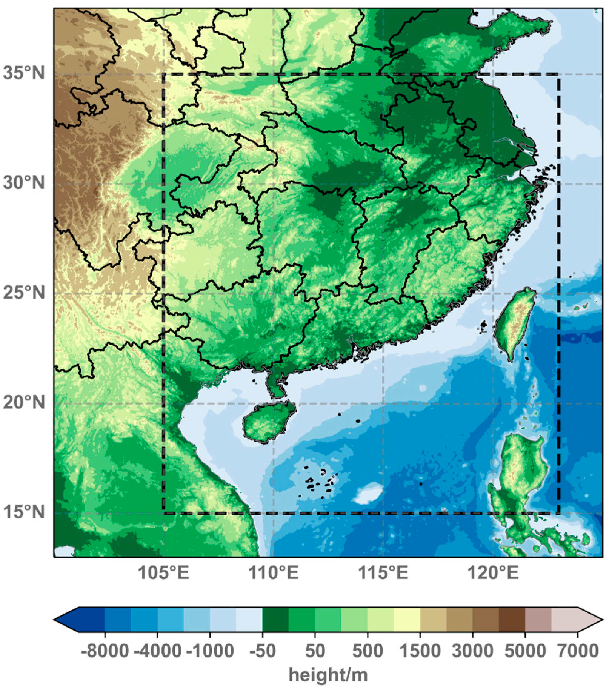
2.1. Data
2.1.1. FY-4A Dataset
2.1.2. Himawari-8 Dataset
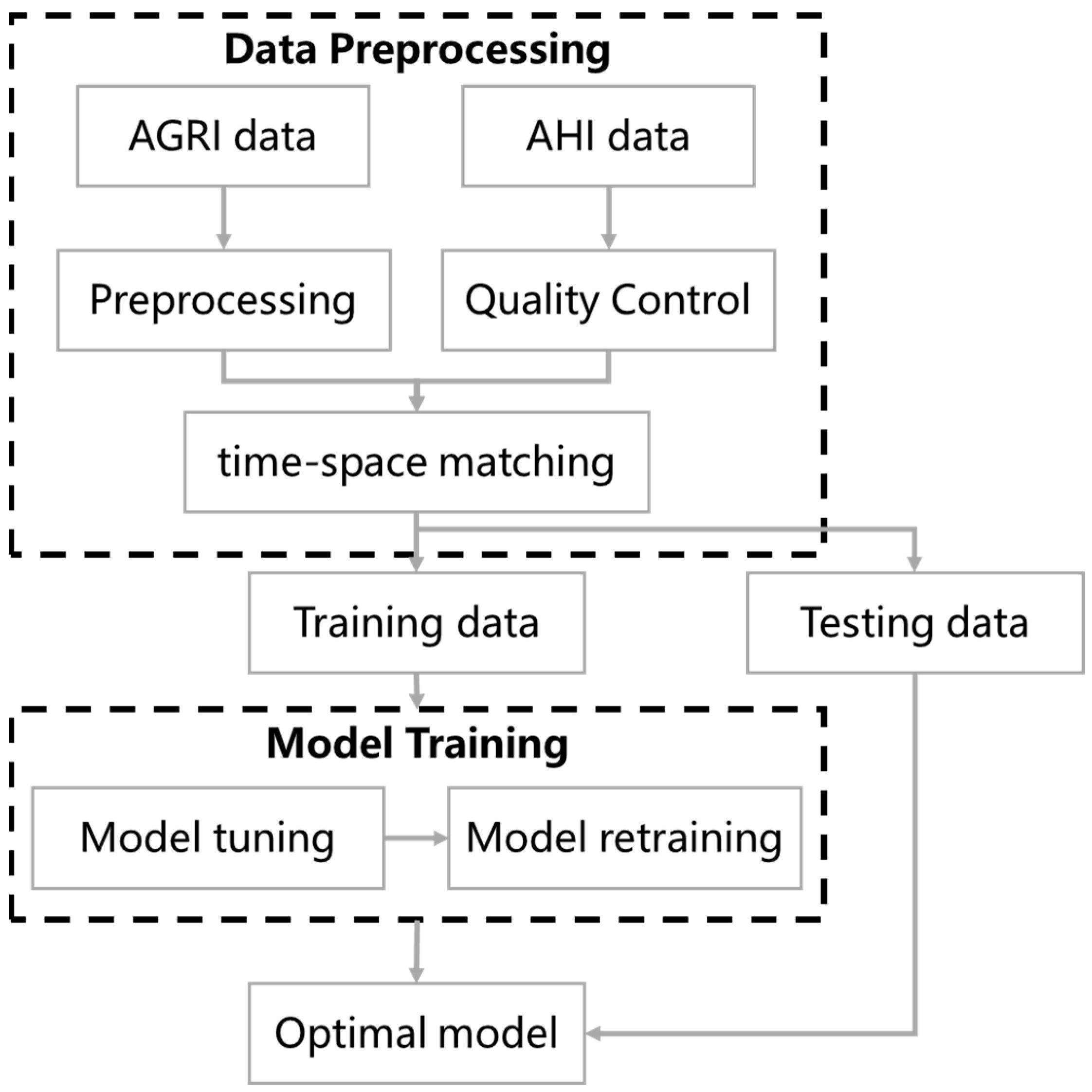
2.2. Data Pre-Processing
2.2.1. AGRI Data Preprocessing
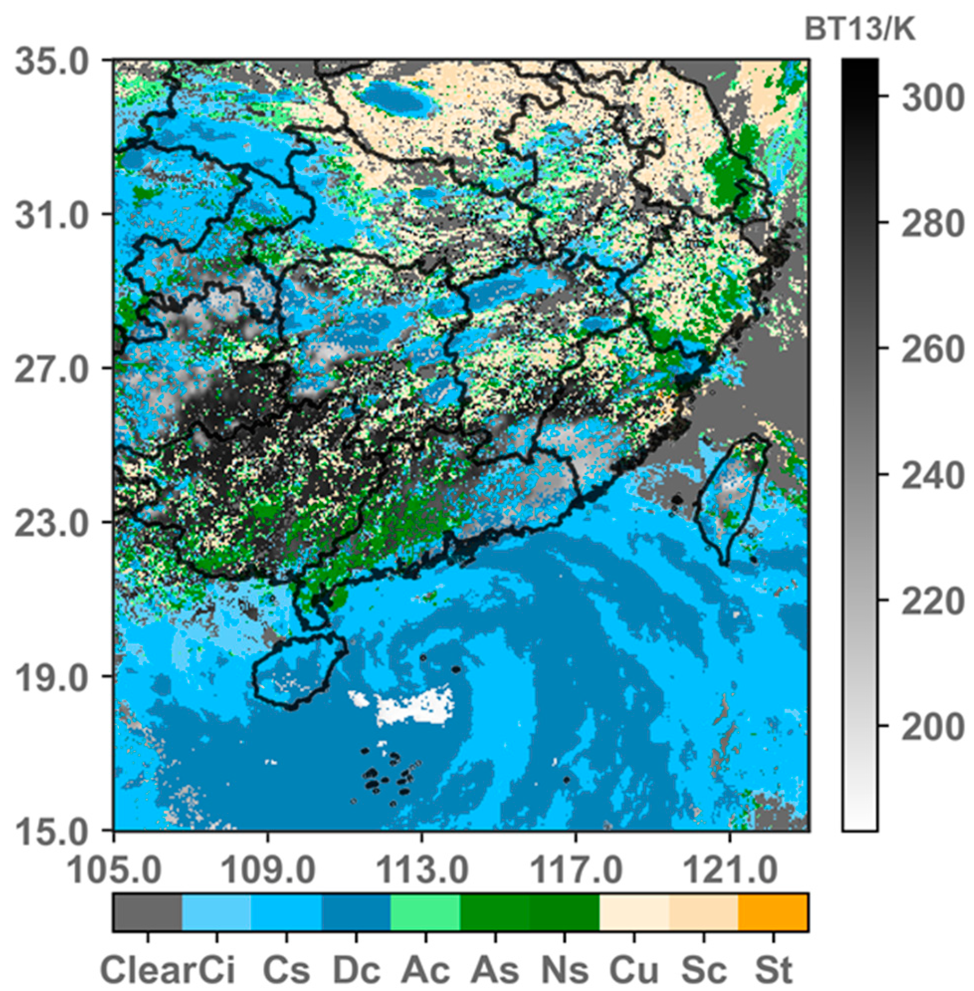
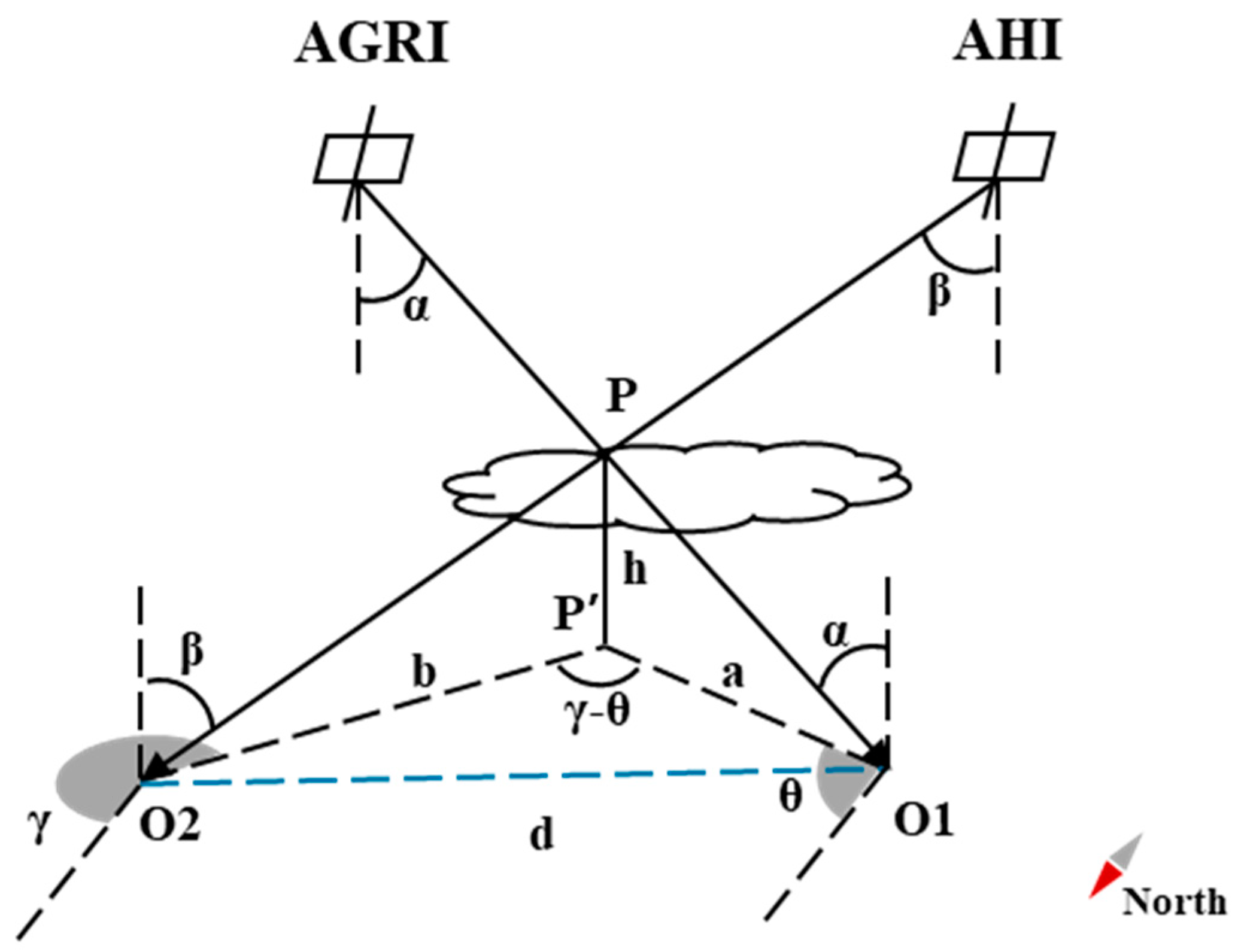
2.2.2. Cloud Type Label Matching
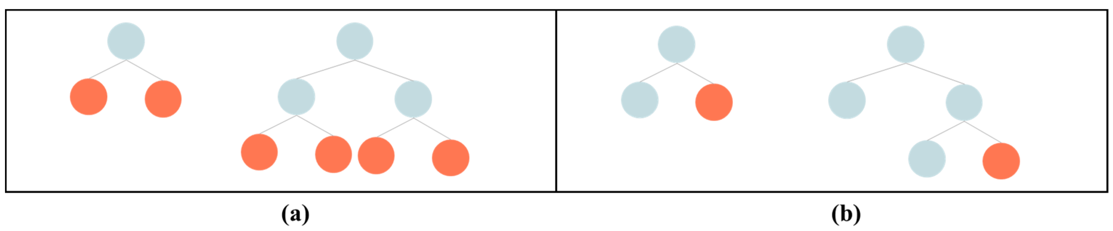
2.3. LightGBM
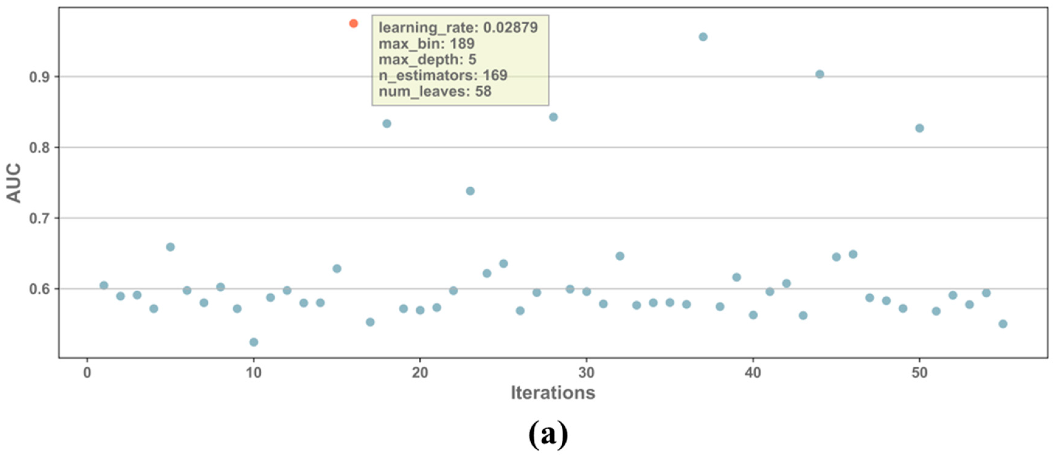
2.4. Bayesian-Optimization
- According to the maximized acquisition function , to find the next set of possible evaluation points, .
- Calculate the corresponding model performance based on the evaluation points .
- Update to the previous observation , and update the probabilistic surrogate model.
2.5. Evaluation Indicators
2.6. Experimental Setup
3. Results
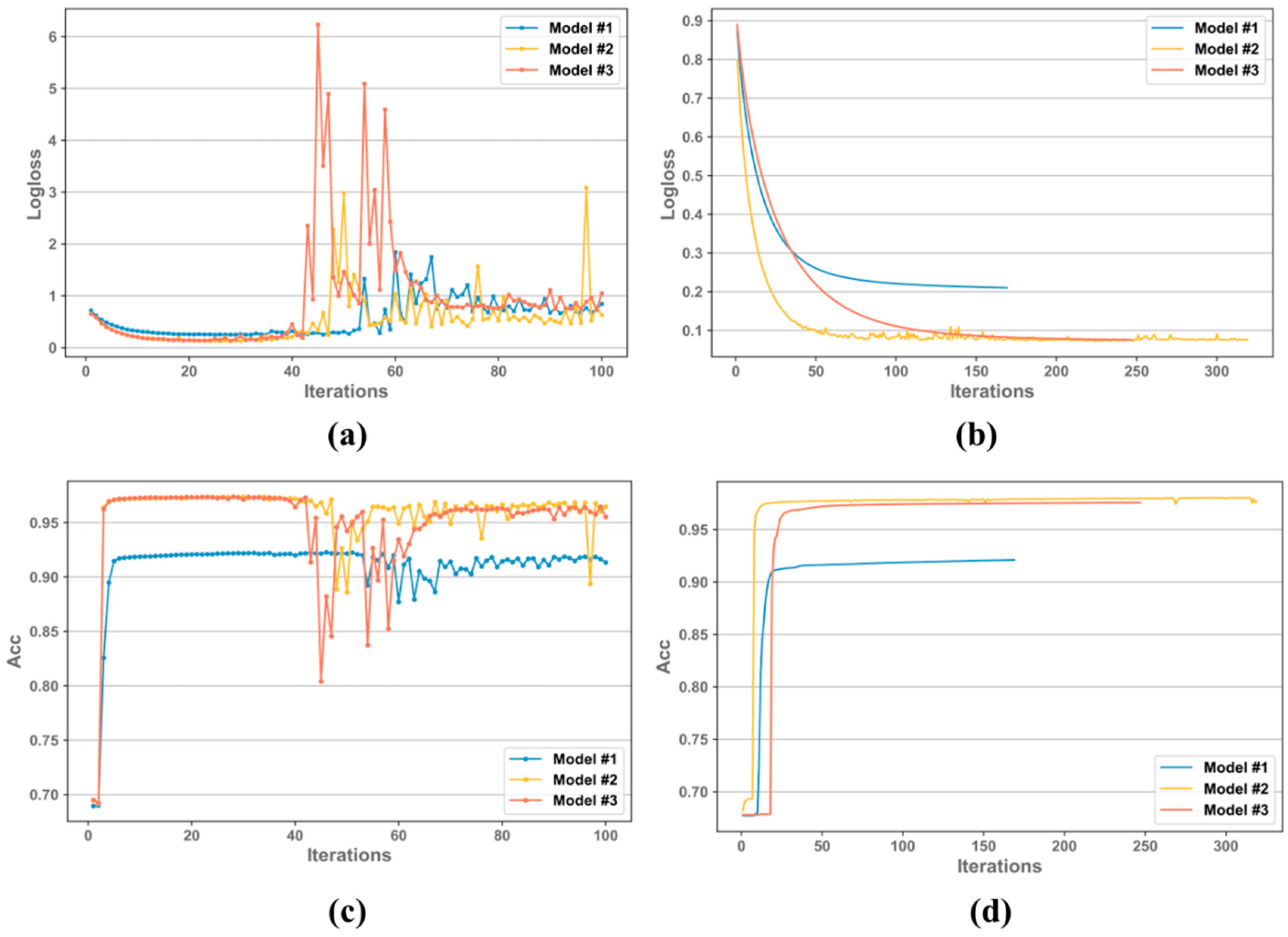
3.1. Model Tuning
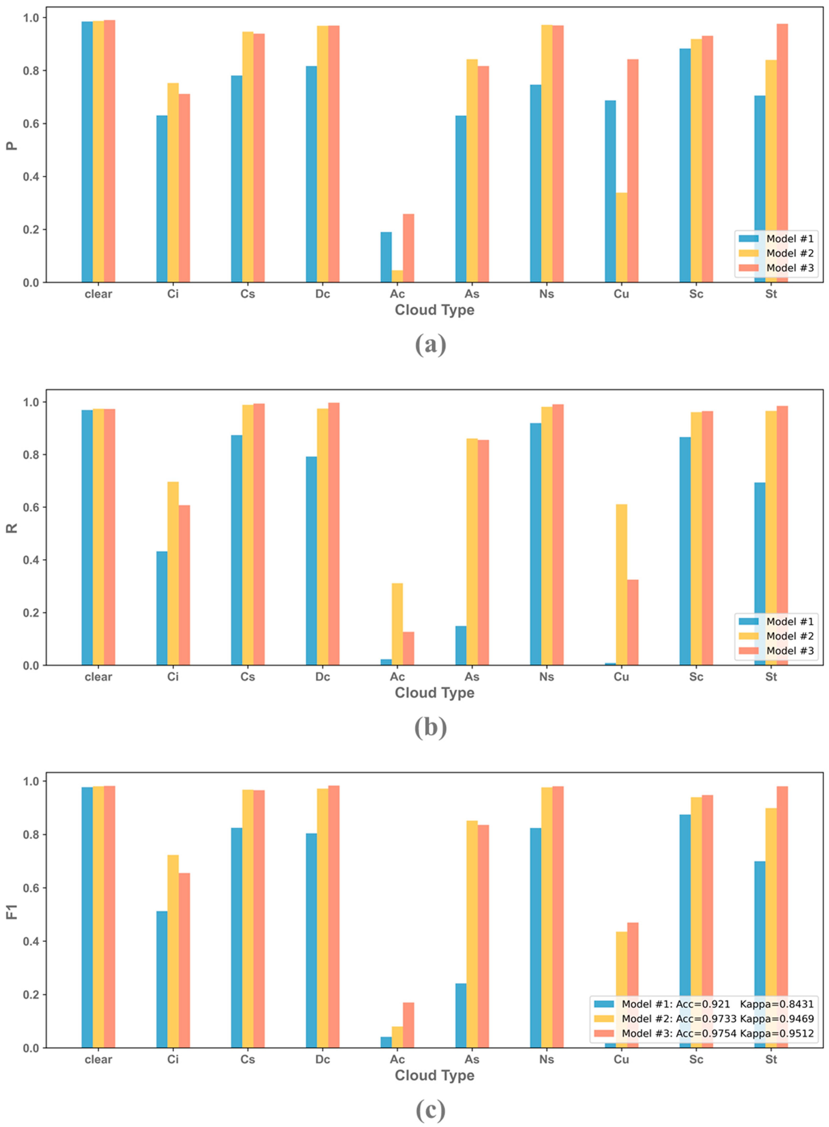
3.2. Comparison of Different Channel Combination Models
3.3. Model Evaluation
3.4. Comparison of Model Accuracy
4. Discussion
- By comparing the performance of the model before and after hyperparameter optimization for the three different input channel combinations, it was demonstrated that Bayesian optimization effectively improved the model performance.
- In evaluating the performance of the different input channel combination models on the testing set, we found that the advantage of the VIS and Shortwave channels in recognizing cloud thickness improved the classification effect of the models to a certain extent, especially the recall of Ac and Cu, which are two types of cloud types with thinner cloud thickness and lower cloud top height. However, because of the spectral similarity between clear and Ac and Cu, caused the model to misclassify clear as these two types of clouds, leading to decreased precision.
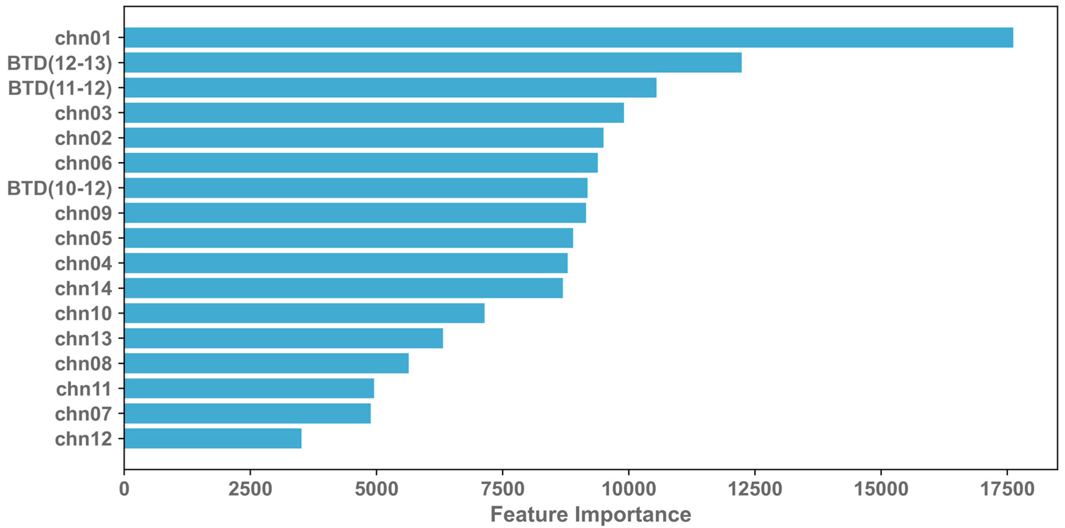
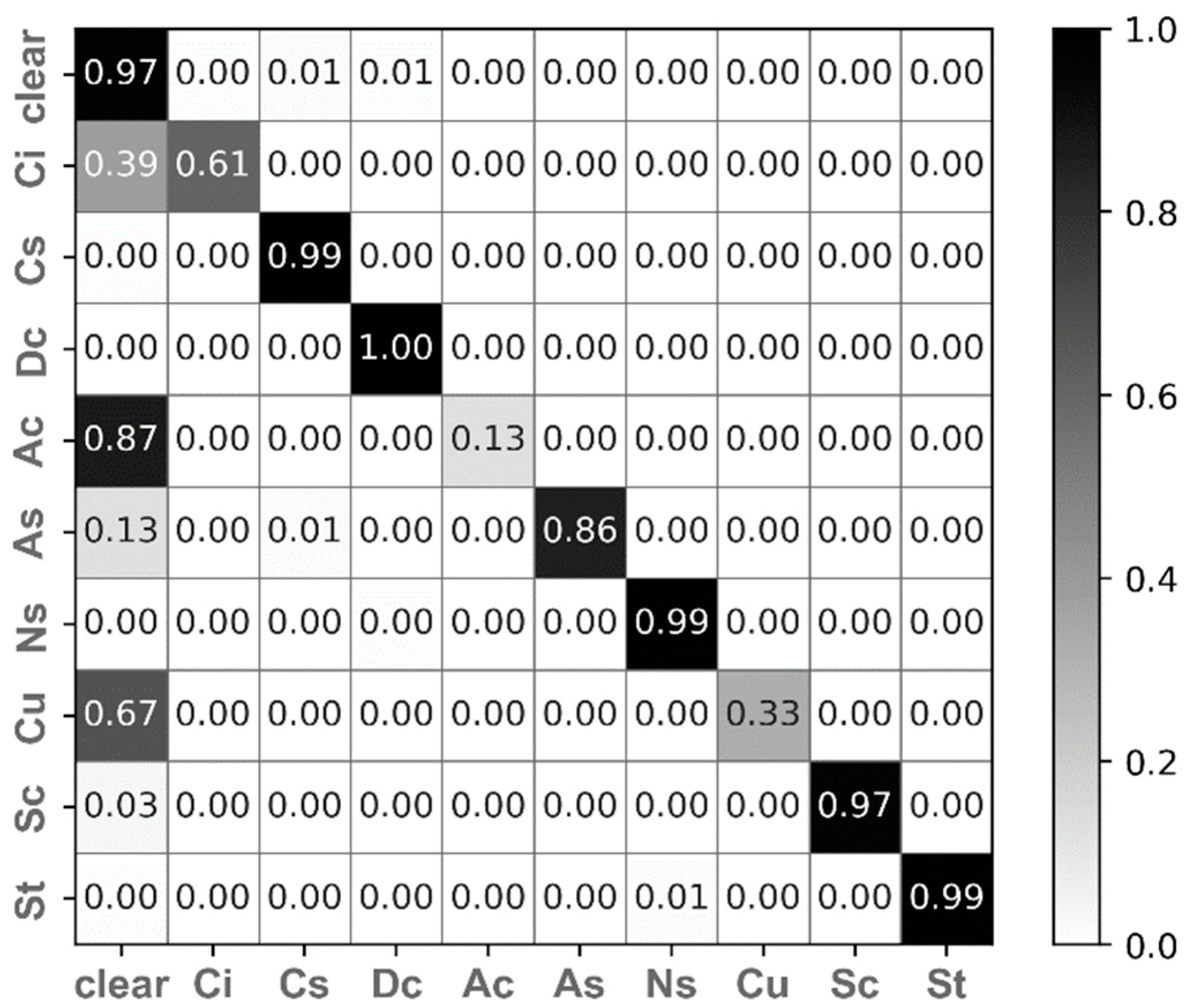
- In evaluating the optimal model, we found that the VIS and Shortwave infrared channels and the brightness temperature difference channel accounted for 43.79% and 21.84% of the overall features, and the top three feature variables in terms of feature importance were the first-channel (0.47 μm) albedo, BTD (12–13), and BTD (11–12). When the model classifies cloud types, it is easy to identify clouds with thinner cloud thickness (Ci, Ac, and Cu) as clear. One reason for this is that Ci, Ac, and Cu clouds tend to be located at the edges of the cloud, which are represented by a smaller number of training samples than other cloud types. This can lead to the model not having enough learning ability for these categories. Additionally, edge clouds are more likely to be impacted by parallax effects, and, even after quality control, there may still be labeling errors that affect the accuracy of the model’s classifications.
5. Conclusions
Author Contributions
Funding
Data Availability Statement
Acknowledgments
Conflicts of Interest
References
- Fernández-Prieto, D.; Van Oevelen, P.; Su, Z.; Wagner, W. Editorial “Advances in Earth Observation for Water Cycle Science”. Hydrol. Earth Syst. Sci. 2012, 16, 543–549. [Google Scholar] [CrossRef]
- Baker, M.B.; Peter, T. Small-Scale Cloud Processes and Climate. Nature 2008, 451, 299–300. [Google Scholar] [CrossRef] [PubMed]
- Bengtsson, L. The Global Atmospheric Water Cycle. Environ. Res. Lett. 2010, 5, 025202. [Google Scholar] [CrossRef]
- Stephens, G.L. Cloud Feedbacks in the Climate System: A Critical Review. J. Clim. 2005, 18, 237–273. [Google Scholar] [CrossRef]
- Huang, J. Effects of Humidity, Aerosol, and Cloud on Subambient Radiative Cooling. Int. J. Heat Mass Transf. 2022, 186, 122438. [Google Scholar] [CrossRef]
- Li, Y.; Fang, L.; Kou, X. Principle and standard of auto-observation cloud classification for satellite, ground measurements and model. Chin. J. Geophys. 2014, 57, 2433–2441. [Google Scholar]
- Forsythe, J.M.; Vonder Haar, T.H.; Reinke, D.L. Cloud-Base Height Estimates Using a Combination of Meteorological Satellite Imagery and Surface Reports. J. Appl. Meteor. 2000, 39, 2336–2347. [Google Scholar] [CrossRef]
- Beusch, L.; Foresti, L.; Gabella, M.; Hamann, U. Satellite-Based Rainfall Retrieval: From Generalized Linear Models to Artificial Neural Networks. Remote Sens. 2018, 6, 939. [Google Scholar] [CrossRef]
- Ren, J.; Xu, G.; Zhang, W.; Leng, L.; Xiao, Y.; Wan, R.; Wang, J. Evaluation and Improvement of FY-4A AGRI Quantitative Precipitation Estimation for Summer Precipitation over Complex Topography of Western China. Remote Sens. 2021, 13, 4366. [Google Scholar] [CrossRef]
- Rucong, Y.; Yongqiang, Y.; Minghua, Z. Comparing Cloud Radiative Properties between the Eastern China and the Indian Monsoon Region. Adv. Atmos. Sci. 2001, 18, 1090–1102. [Google Scholar] [CrossRef]
- Duan, A.; Hu, D.; Hu, W.; Zhang, P. Precursor Effect of the Tibetan Plateau Heating Anomaly on the Seasonal March of the East Asian Summer Monsoon Precipitation. JGR Atmos. 2020, 125, e2020JD032948. [Google Scholar] [CrossRef]
- Chiang, J.C.H.; Kong, W.; Wu, C.H.; Battisti, D.S. Origins of East Asian Summer Monsoon Seasonality. J. Clim. 2020, 33, 7945–7965. [Google Scholar] [CrossRef]
- Yihui, D.; Chan, J.C.L. The East Asian Summer Monsoon: An Overview. Meteorol. Atmos. Phys. 2005, 89, 117–142. [Google Scholar] [CrossRef]
- Doswell, C.A. Severe Convective Storms—An Overview. In Meteorological Monographs; Springer: Berlin/Heidelberg, Germany, 2001; Volume 50, pp. 1–26. [Google Scholar] [CrossRef]
- Schiffer, R.A.; Rossow, W.B. The International Satellite Cloud Climatology Project (ISCCP): The First Project of the World Climate Research Programme. Bull. Am. Meteorol. Soc. 1983, 64, 779–784. [Google Scholar] [CrossRef]
- Tapakis, R.; Charalambides, A.G. Equipment and Methodologies for Cloud Detection and Classification: A Review. Sol. Energy 2013, 95, 392–430. [Google Scholar] [CrossRef]
- Inoue, T. A Cloud Type Classification with NOAA 7 Split-Window Measurements. J. Geophys. Res. 1987, 92, 3991. [Google Scholar] [CrossRef]
- Lutz, H.-J.; Inoue, T.; Schmetz, J. Comparison of a Split-Window and a Multi-Spectral Cloud Classification for MODIS Observations. J. Meteorol. Soc. Jpn. 2003, 81, 623–631. [Google Scholar] [CrossRef]
- Purbantoro, B.; Aminuddin, J.; Manago, N.; Toyoshima, K.; Lagrosas, N.; Sumantyo, J.T.S.; Kuze, H. Comparison of Cloud Type Classification with Split Window Algorithm Based on Different Infrared Band Combinations of Himawari-8 Satellite. ARS 2018, 7, 218–234. [Google Scholar] [CrossRef]
- Christodoulou, C.I.; Michaelides, S.C.; Pattichis, C.S. Multifeature Texture Analysis for the Classification of Clouds in Satellite Imagery. IEEE Trans. Geosci. Remote Sens. 2003, 41, 2662–2668. [Google Scholar] [CrossRef]
- Zhang, C.; Zhuge, X.; Yu, F. Development of a High Spatiotemporal Resolution Cloud-Type Classification Approach Using Himawari-8 and CloudSat. Int. J. Remote Sens. 2019, 40, 6464–6481. [Google Scholar] [CrossRef]
- Azimi-Sadjadi, M.R.; Zekavat, S.A. Cloud Classification Using Support Vector Machines. In Proceedings of the IGARSS 2000. IEEE 2000 International Geoscience and Remote Sensing Symposium. Taking the Pulse of the Planet: The Role of Remote Sensing in Managing the Environment. Proceedings (Cat. No.00CH37120), Honolulu, HI, USA, 24–28 July 2000; Volume 2, pp. 669–671. [Google Scholar]
- Liu, C.; Yang, S.; Di, D.; Yang, Y.; Zhou, C.; Hu, X.; Sohn, B.-J. A Machine Learning-Based Cloud Detection Algorithm for the Himawari-8 Spectral Image. Adv. Atmos. Sci. 2022, 39, 1994–2007. [Google Scholar] [CrossRef]
- Jiang, Y.; Cheng, W.; Gao, F.; Zhang, S.; Wang, S.; Liu, C.; Liu, J. A Cloud Classification Method Based on a Convolutional Neural Network for FY-4A Satellites. Remote Sens. 2022, 14, 2314. [Google Scholar] [CrossRef]
- Li, T.; Wu, D.; Wang, L.; Yu, X. Recognition Algorithm for Deep Convective Clouds Based on FY4A. Neural Comput. Applic 2022, 34, 21067–21088. [Google Scholar] [CrossRef]
- Ke, G.; Meng, Q.; Finley, T.; Wang, T.; Chen, W.; Ma, W.; Ye, Q.; Liu, T.-Y. LightGBM: A Highly Efficient Gradient Boosting Decision Tree. In Advances in Neural Information Processing Systems, Proceedings of the NIPS 2017, Long Beach, CA, USA, 4–9 December 2017; pp. 3149–3157. [CrossRef]
- Lin, N.; Zhang, D.; Feng, S.; Ding, K.; Tan, L.; Wang, B.; Chen, T.; Li, W.; Dai, X.; Pan, J.; et al. Rapid Landslide Extraction from High-Resolution Remote Sensing Images Using SHAP-OPT-XGBoost. Remote Sens. 2023, 15, 3901. [Google Scholar] [CrossRef]
- Dai, J.; Liu, T.; Zhao, Y.; Tian, S.; Ye, C.; Nie, Z. Remote Sensing Inversion of the Zabuye Salt Lake in Tibet, China Using LightGBM Algorithm. Front. Earth Sci. 2023, 10, 1022280. [Google Scholar] [CrossRef]
- Zhong, J.; Zhang, X.; Gui, K.; Wang, Y.; Che, H.; Shen, X.; Zhang, L.; Zhang, Y.; Sun, J.; Zhang, W. Robust Prediction of Hourly PM2.5 from Meteorological Data Using LightGBM. Natl. Sci. Rev. 2021, 8, nwaa307. [Google Scholar] [CrossRef]
- Zhang, P.; Zhu, L.; Tang, S.; Gao, L.; Chen, L.; Zheng, W.; Han, X.; Chen, J.; Shao, J. General Comparison of FY-4A/AGRI with Other GEO/LEO Instruments and Its Potential and Challenges in Non-Meteorological Applications. Front. Earth Sci. 2019, 6, 224. [Google Scholar] [CrossRef]
- Letu, H.; Nagao, T.M.; Nakajima, T.Y.; Riedi, J.; Ishimoto, H.; Baran, A.J.; Shang, H.; Sekiguchi, M.; Kikuchi, M. Ice Cloud Properties from Himawari-8/AHI Next-Generation Geostationary Satellite: Capability of the AHI to Monitor the DC Cloud Generation Process. IEEE Trans. Geosci. Remote Sens. 2019, 57, 3229–3239. [Google Scholar] [CrossRef]
- Rossow, W.B.; Schiffer, R.A. Advances in Understanding Clouds from ISCCP. Bull. Am. Meteorol. Soc. 1999, 80, 2261–2287. [Google Scholar] [CrossRef]
- Kim, M.; Kim, J.; Lim, H.; Lee, S.; Cho, Y.; Yeo, H.; Kim, S.-W. Exploring Geometrical Stereoscopic Aerosol Top Height Retrieval from Geostationary Satellite Imagery in East Asia. Atmos. Meas. Tech. 2023, 16, 2673–2690. [Google Scholar] [CrossRef]
- Brochu, E.; Cora, V.M.; de Freitas, N. A Tutorial on Bayesian Optimization of Expensive Cost Functions, with Application to Active User Modeling and Hierarchical Reinforcement Learning. 2010. Available online: https://www.cs.ox.ac.uk/publications/publication7472-abstract.html (accessed on 19 September 2023).
- Brusca, S.; Famoso, F.; Lanzafame, R.; Messina, M.; Monforte, P. Placement Optimization of Biodiesel Production Plant by Means of Centroid Mathematical Method. Energy Procedia 2017, 126, 353–360. [Google Scholar] [CrossRef]
- Hao, X.; Zhang, Z.; Xu, Q.; Huang, G.; Wang, K. Prediction of F-CaO Content in Cement Clinker: A Novel Prediction Method Based on LightGBM and Bayesian Optimization. Chemom. Intell. Lab. Syst. 2022, 220, 104461. [Google Scholar] [CrossRef]
- Mohajerani, S.; Saeedi, P. Cloud-Net: An End-To-End Cloud Detection Algorithm for Landsat 8 Imagery. In Proceedings of the IGARSS 2019–2019 IEEE International Geoscience and Remote Sensing Symposium, Yokohama, Japan, 28 July–2 August 2019; pp. 1029–1032. [Google Scholar]
- Jeppesen, J.H.; Jacobsen, R.H.; Inceoglu, F.; Toftegaard, T.S. A Cloud Detection Algorithm for Satellite Imagery Based on Deep Learning. Remote Sens. Environ. 2019, 229, 247–259. [Google Scholar] [CrossRef]
- Yu, Z.; Ma, S.; Han, D.; Li, G.; Gao, D.; Yan, W. A Cloud Classification Method Based on Random Forest for FY-4A. Int. J. Remote Sens. 2021, 42, 3353–3379. [Google Scholar] [CrossRef]
- Wang, B.; Zhou, M.; Cheng, W.; Chen, Y.; Sheng, Q.; Li, J.; Wang, L. An Efficient Cloud Classification Method Based on a Densely Connected Hybrid Convolutional Network for FY-4A. Remote Sens. 2023, 15, 2673. [Google Scholar] [CrossRef]
- Xie, L.; Zhang, R.; Zhan, J.; Li, S.; Shama, A.; Zhan, R.; Wang, T.; Lv, J.; Bao, X.; Wu, R. Wildfire Risk Assessment in Liangshan Prefecture, China Based on An Integration Machine Learning Algorithm. Remote Sens. 2022, 14, 4592. [Google Scholar] [CrossRef]
- Liu, J.; Li, Y. Cloud phase detection algorithm for geostationary satellite data: Cloud phase detection algorithm for geostationary satellite data. J. Infrared Millim. Waves 2012, 30, 322–327. [Google Scholar] [CrossRef]


| Band | Spectral Coverage | Central Wavelength | Spectral Bandwidth | Main Applications |
|---|---|---|---|---|
| 1 | VIS/NIR | 0.47 µm | 0.45~0.49 µm | Aerosol, visibility |
| 2 | 0.65 µm | 0.55~0.75 µm | Fog and cloud | |
| 3 | 0.825 µm | 0.75~0.90 µm | Vegetation | |
| 4 | Shortwave IR | 1.375 µm | 1.36~1.39 µm | Cirrus cloud |
| 5 | 1.61 µm | 1.58~1.64 µm | Cloud and snow | |
| 6 | 2.25 µm | 2.1~2.35 µm | Cirrus clouds and aerosol | |
| 7 | Midwave IR | 3.75 µm | 3.5~4.0 µm | Fire point |
| 8 | 3.75 µm | 3.5~4.0 µm | Earth’s surface | |
| 9 | Water vapor | 6.25 µm | 5.8~6.7 µm | Upper-level WV |
| 10 | 7.1 µm | 6.9~7.3 µm | Mid-level WV | |
| 11 | Longwave IR | 8.5 µm | 8.0~9.0 µm | Cloud motion wind and cloud |
| 12 | 10.7 µm | 10.3~11.3 µm | Sea surface temperature | |
| 13 | 12.0 µm | 11.5~12.5 µm | Sea surface temperature | |
| 14 | 13.5 µm | 13.2~13.8 µm | Cloud top height |
| No. | Channel Combinations |
|---|---|
| 1 | Chn07~Chn14 |
| 2 | Chn01~chn14 |
| 3 | Chn01~chn14+ BTD (10−12) + BTD (11−12) + BTD (12−13) |
| Algorithms | Macro P | Macro R | Macro F1 | Acc | Kappa |
|---|---|---|---|---|---|
| LightGBM | 84.10% | 78.24% | 79.74% | 97.54% | 0.951 |
| TT | 26.60% | 31.20% | 22.92% | 51.06% | 0.351 |
| SVM | 70.00% | 56.98% | 59.63% | 96.47% | 0.929 |
| RF | 73.11% | 73.03% | 72.97% | 97.49% | 0.950 |
Disclaimer/Publisher’s Note: The statements, opinions and data contained in all publications are solely those of the individual author(s) and contributor(s) and not of MDPI and/or the editor(s). MDPI and/or the editor(s) disclaim responsibility for any injury to people or property resulting from any ideas, methods, instructions or products referred to in the content. |
© 2023 by the authors. Licensee MDPI, Basel, Switzerland. This article is an open access article distributed under the terms and conditions of the Creative Commons Attribution (CC BY) license (https://creativecommons.org/licenses/by/4.0/).
Share and Cite
Lin, J.; Bao, Y.; Petropoulos, G.P.; Mehraban, A.; Pang, F.; Liu, W. Cloud-Type Classification for Southeast China Based on Geostationary Orbit EO Datasets and the LighGBM Model. Remote Sens. 2023, 15, 5660. https://doi.org/10.3390/rs15245660
Lin J, Bao Y, Petropoulos GP, Mehraban A, Pang F, Liu W. Cloud-Type Classification for Southeast China Based on Geostationary Orbit EO Datasets and the LighGBM Model. Remote Sensing. 2023; 15(24):5660. https://doi.org/10.3390/rs15245660
Chicago/Turabian StyleLin, Jianan, Yansong Bao, George P. Petropoulos, Abouzar Mehraban, Fang Pang, and Wei Liu. 2023. "Cloud-Type Classification for Southeast China Based on Geostationary Orbit EO Datasets and the LighGBM Model" Remote Sensing 15, no. 24: 5660. https://doi.org/10.3390/rs15245660
APA StyleLin, J., Bao, Y., Petropoulos, G. P., Mehraban, A., Pang, F., & Liu, W. (2023). Cloud-Type Classification for Southeast China Based on Geostationary Orbit EO Datasets and the LighGBM Model. Remote Sensing, 15(24), 5660. https://doi.org/10.3390/rs15245660