
A Green Fingerprint of Antarctica: Drones, Hyperspectral Imaging, and Machine Learning for Moss and Lichen Classification

 , , , , and
Abstract
:1. Introduction
- The introduction of a unique workflow that amalgamates UAVs, MSI and HSI data, and ML classifiers for vegetation mapping in Antarctica.
- The development of a series of innovative spectral indices to amplify the classification precision of Antarctic vegetation.
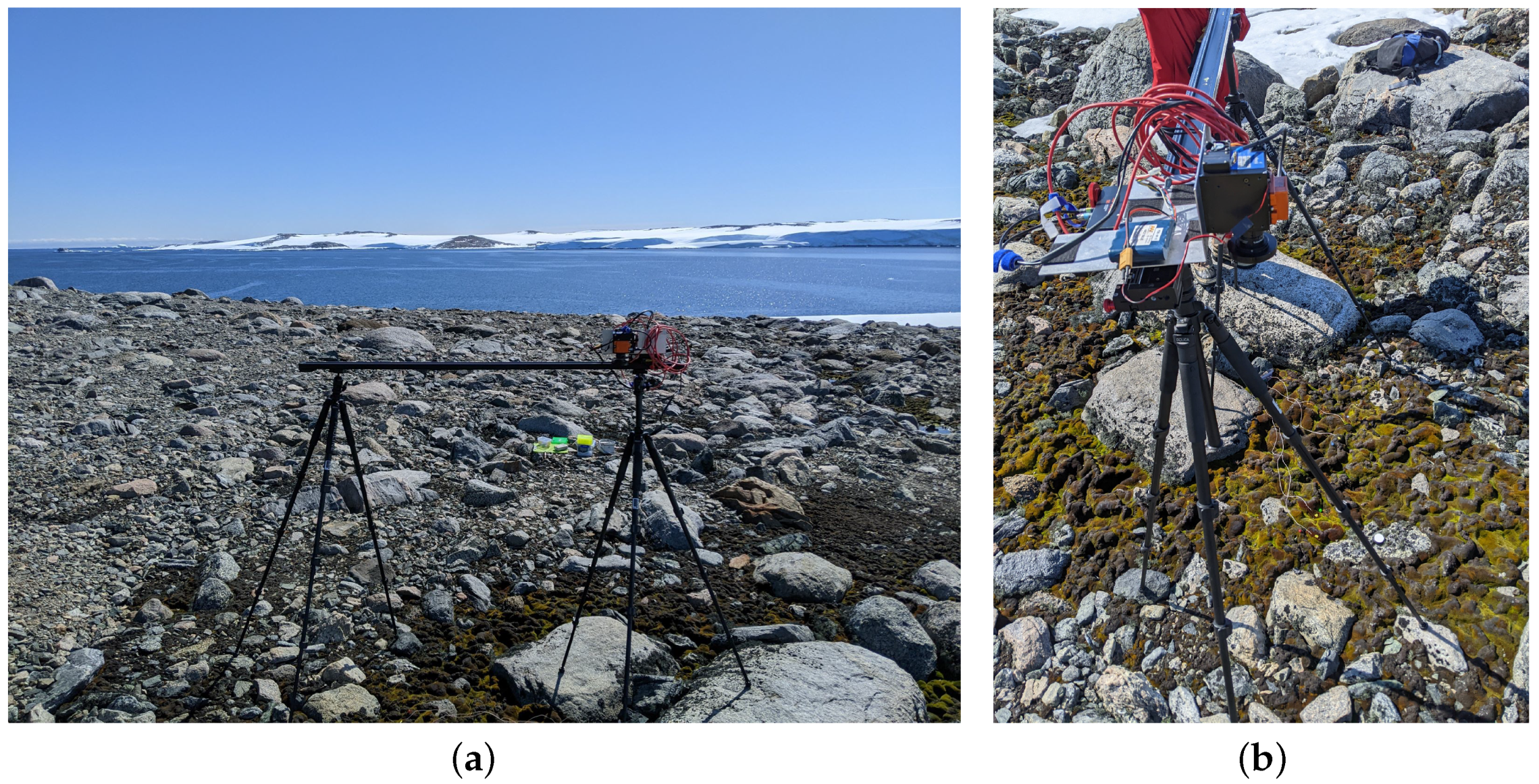
- The execution of a field experiment in ASPA 135 to gather aerial and ground data via custom-built UAVs and HSI cameras.
- The achievement of high accuracy results (95% to 98%) in lichen detection and the classification of moss health using XGBoost models.
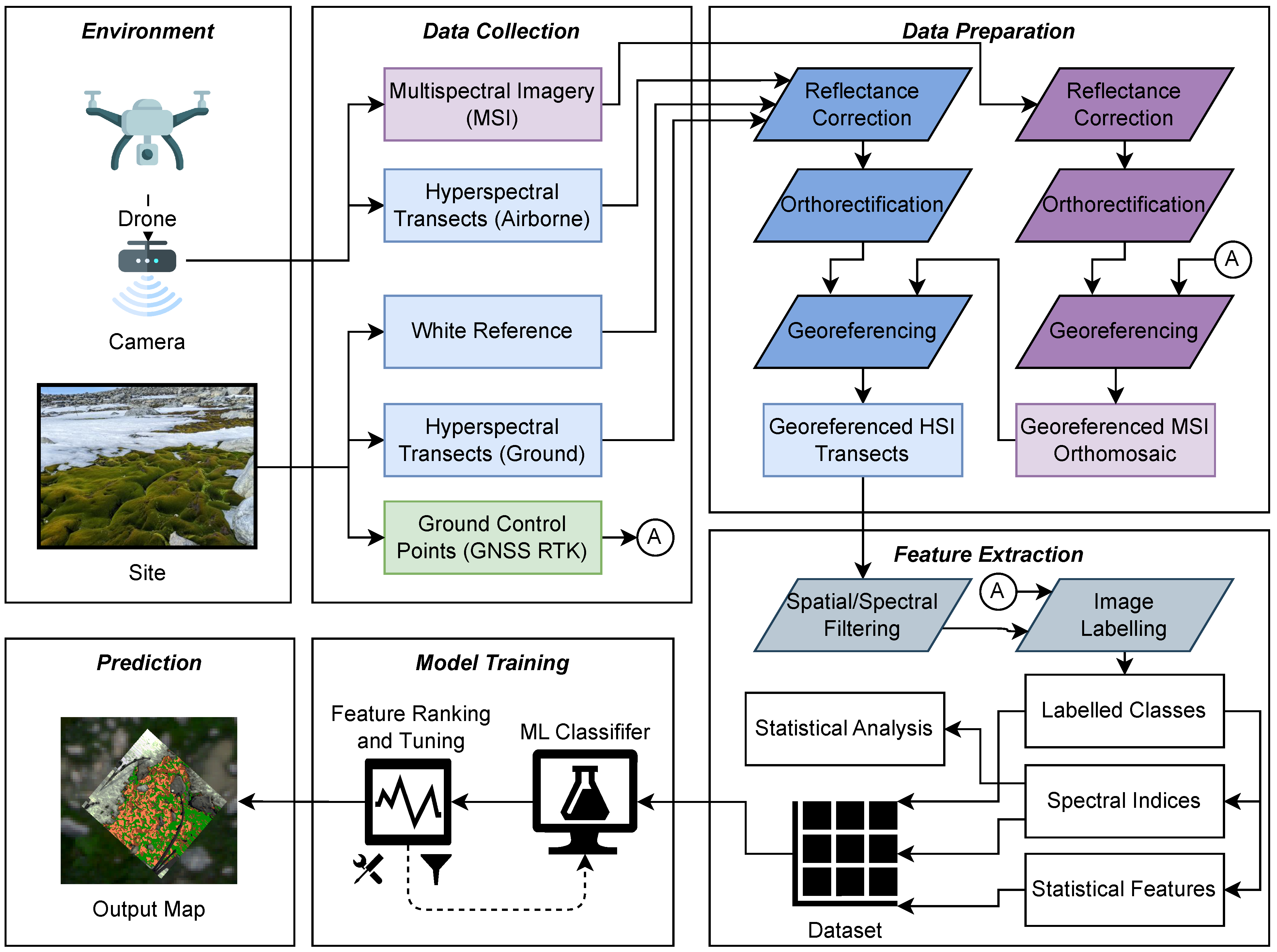
2. Remote Sensing Workflow
2.1. Data Collection
2.2. Data Preparation
2.3. Feature Extraction
2.4. Model Training
2.5. Prediction
3. Methods and Tools
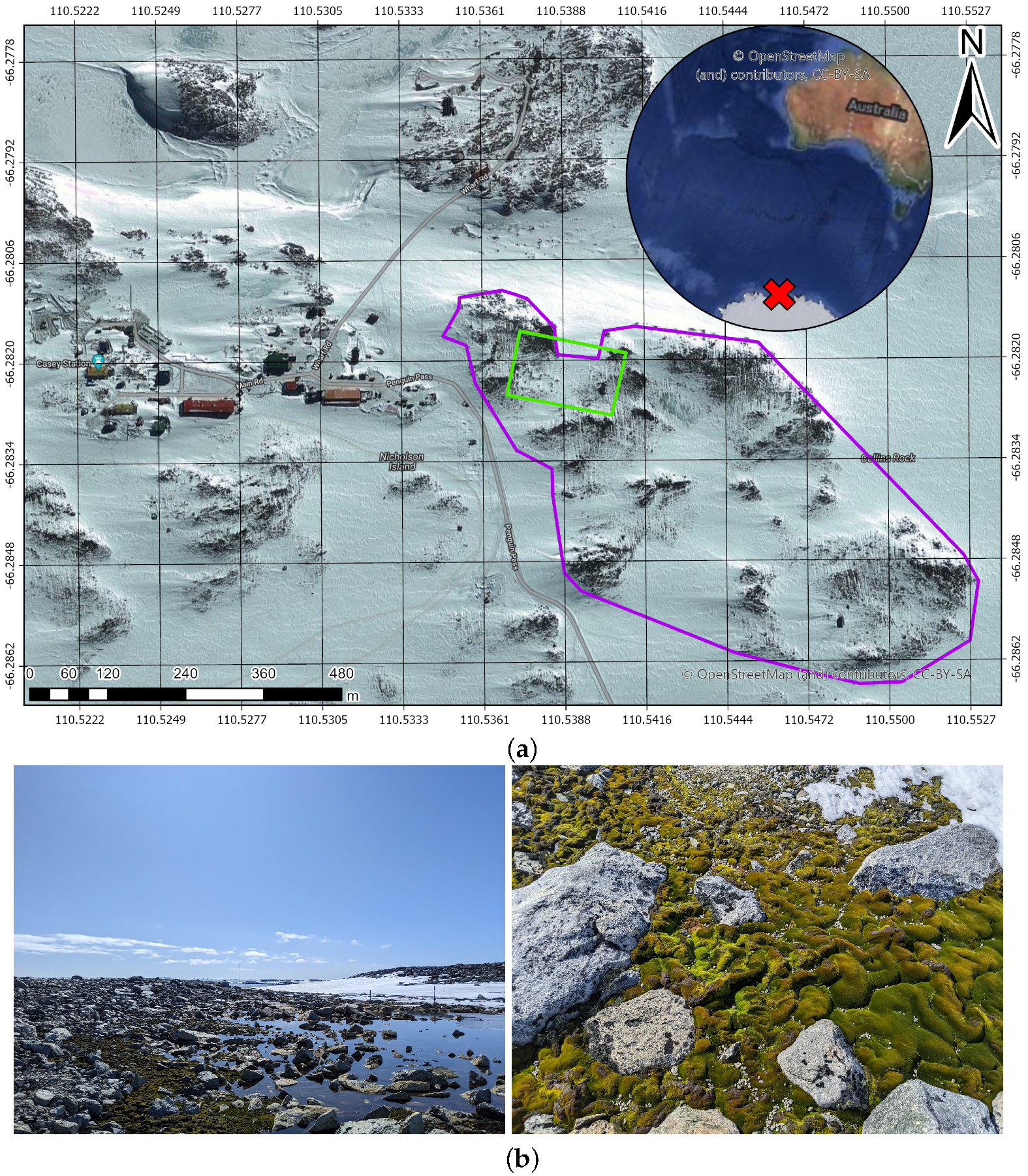
3.1. Site
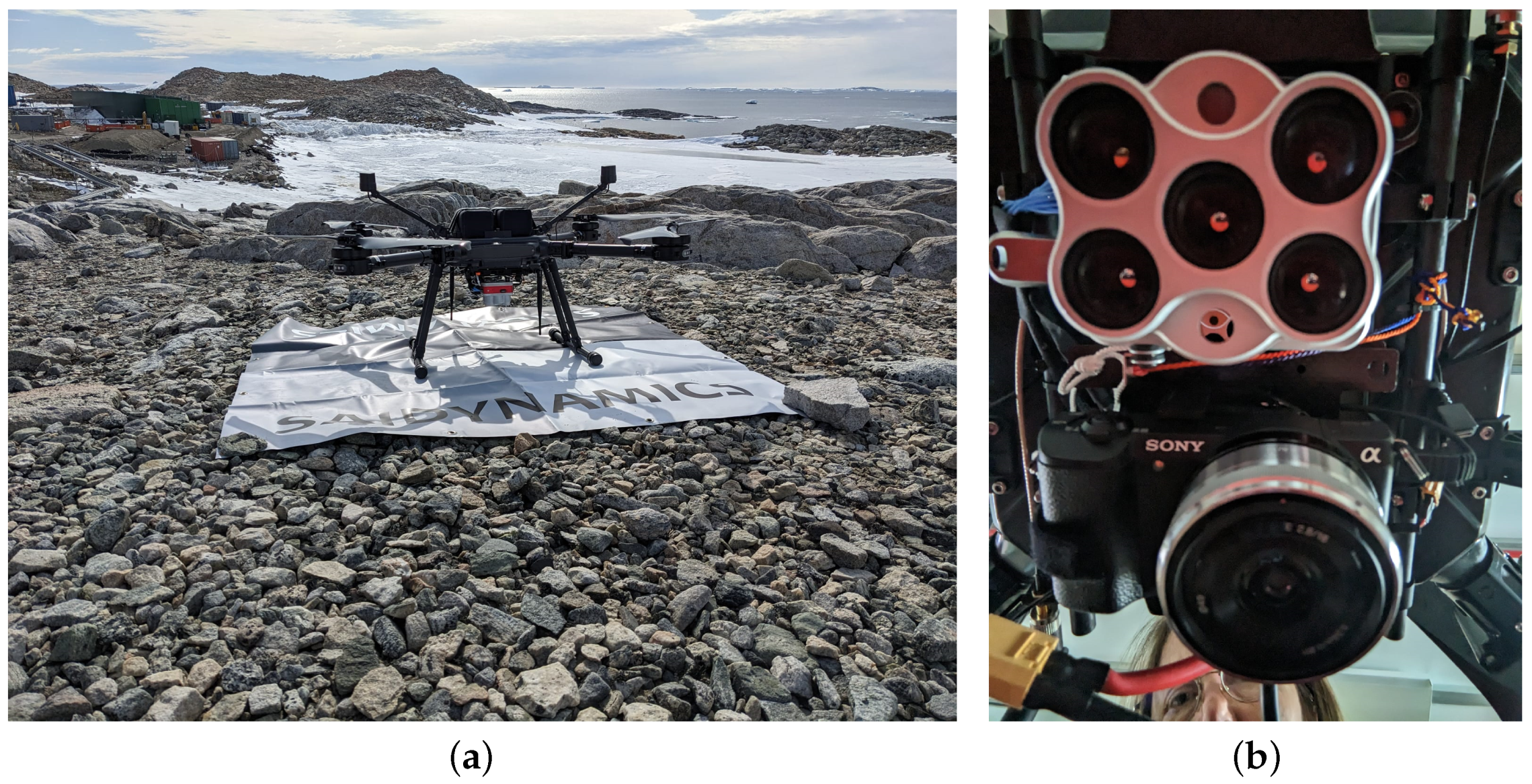
3.2. Aerial Data Collection
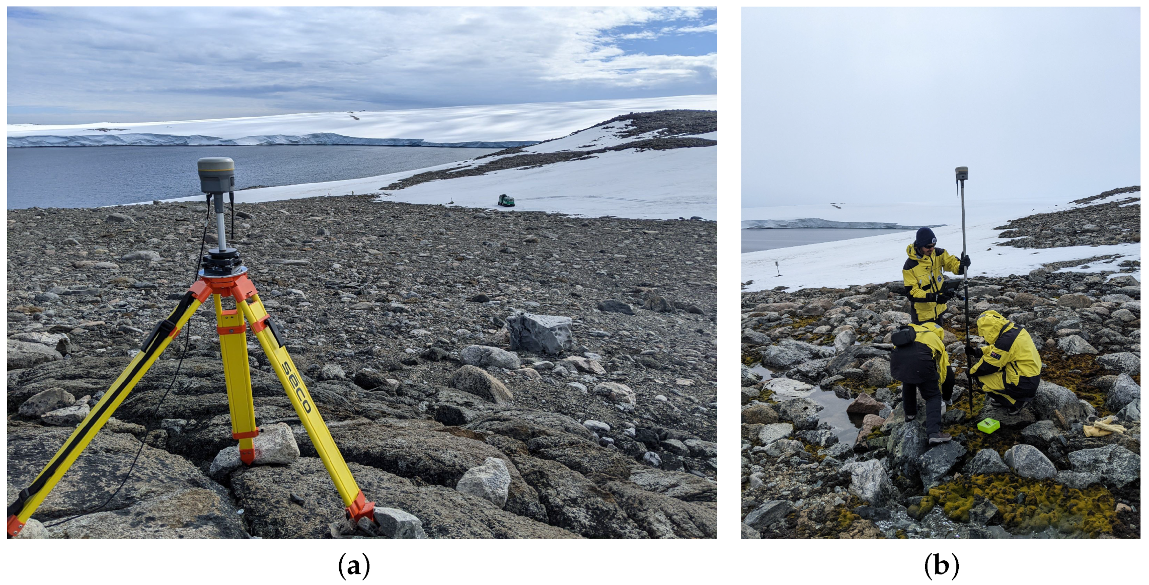
3.3. Ground Data Collection
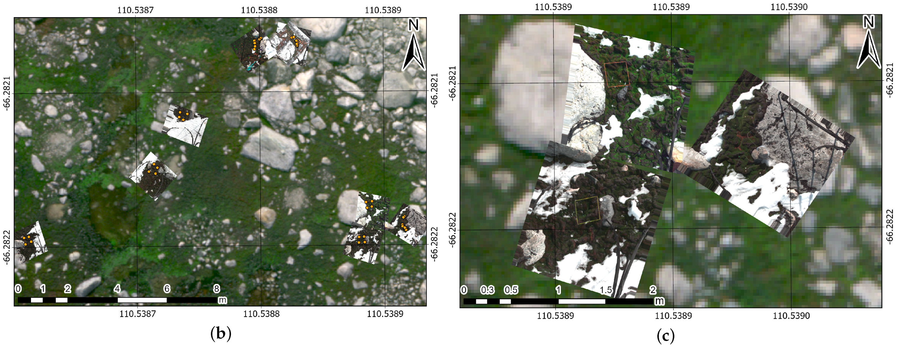
3.4. MSI and HSI Georeferenced Mosaics
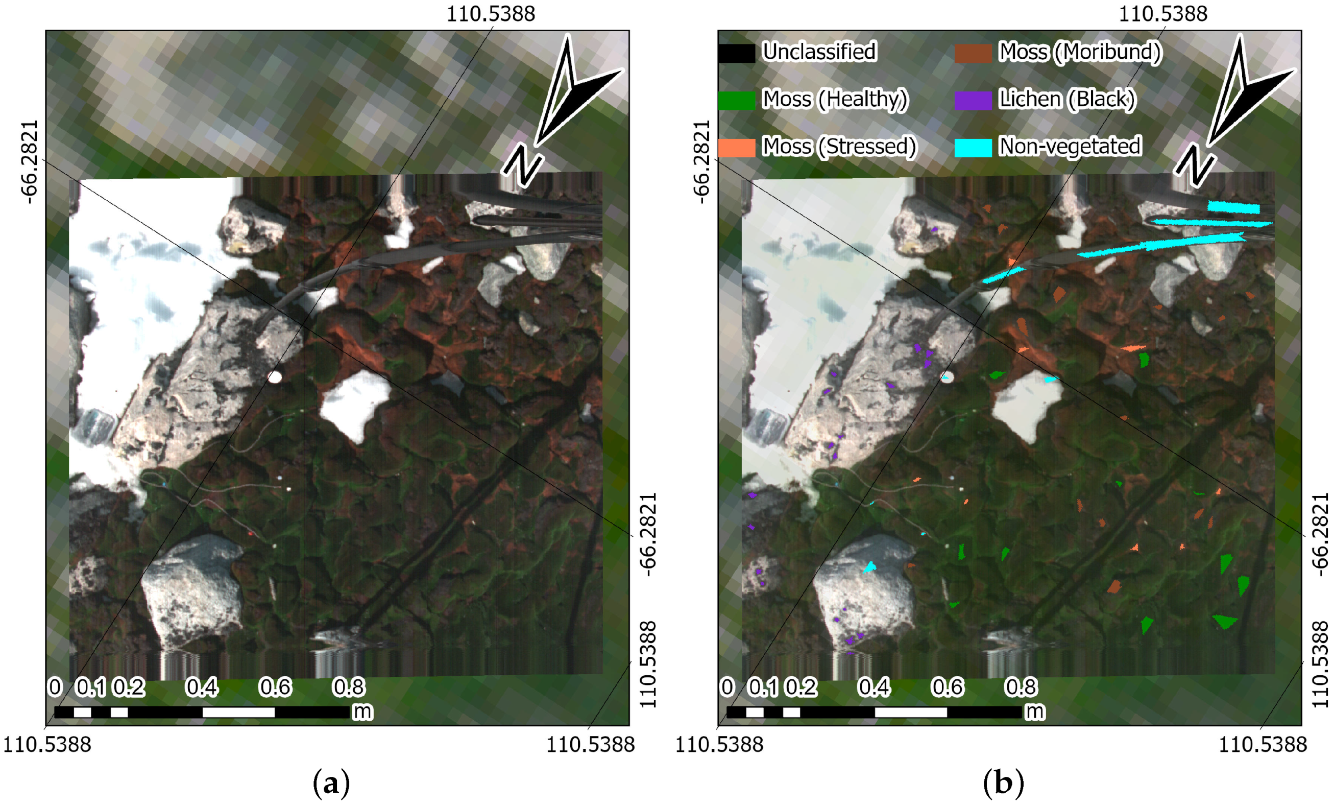
3.5. Training Sampling of HSI Scans
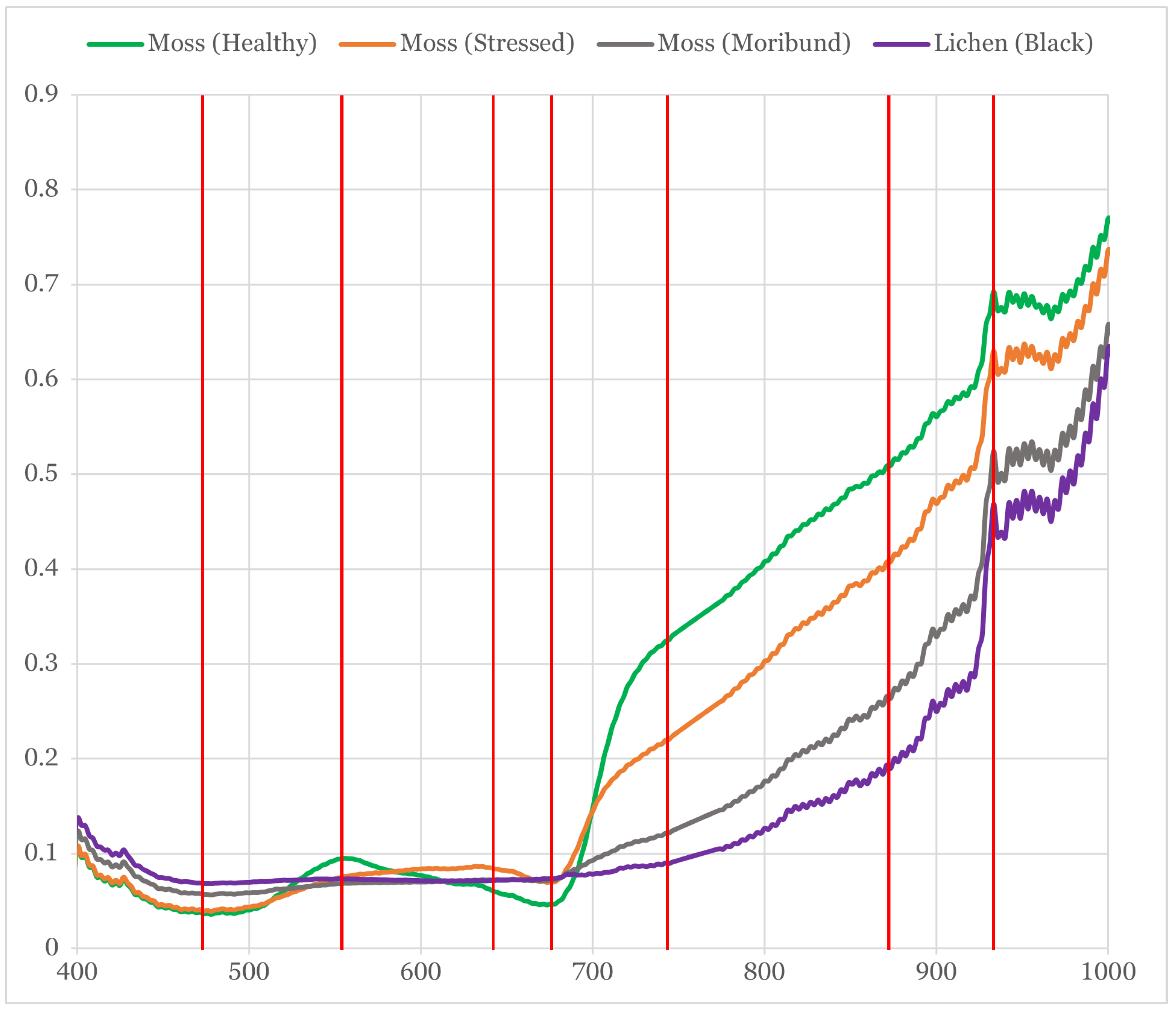
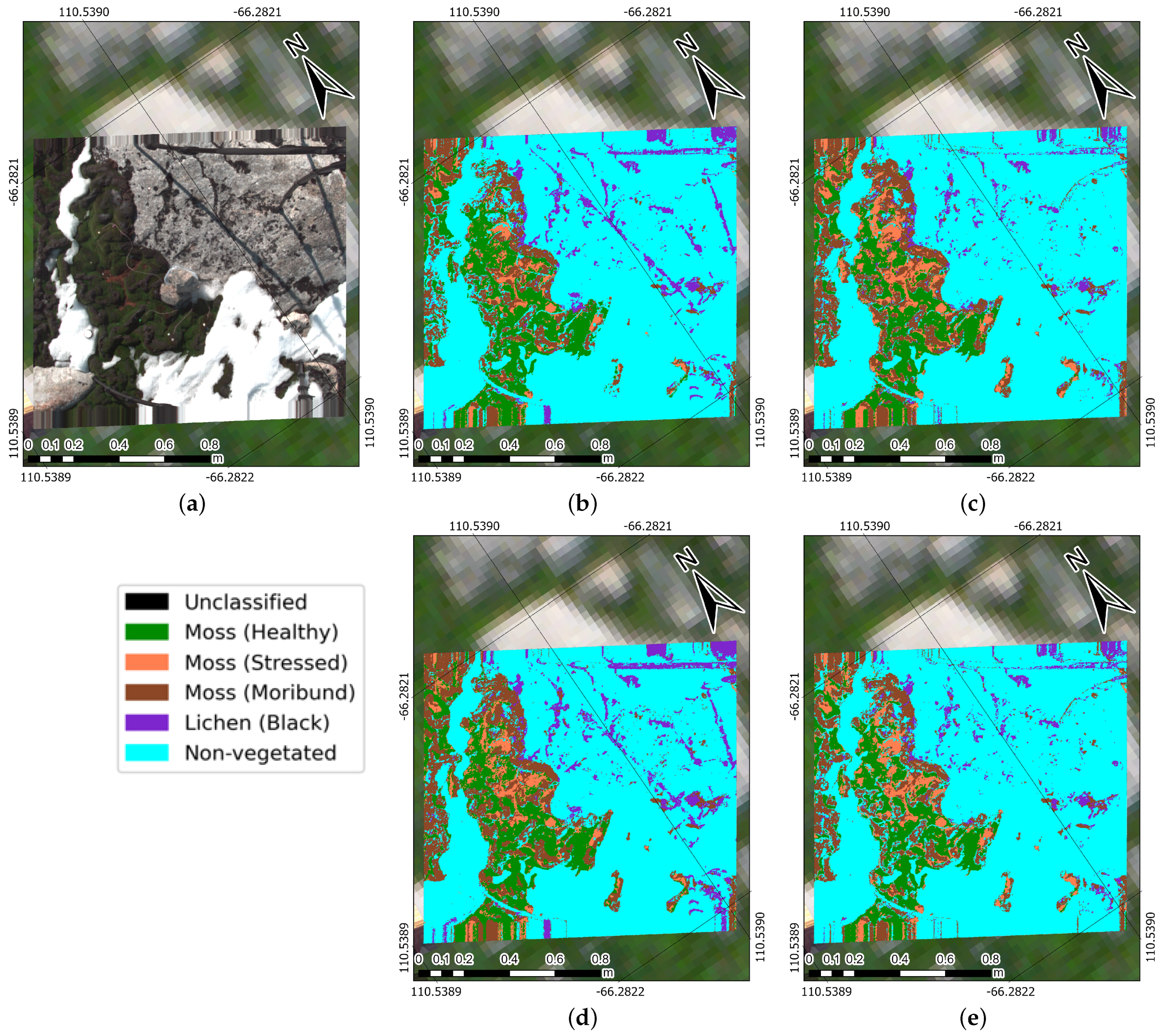
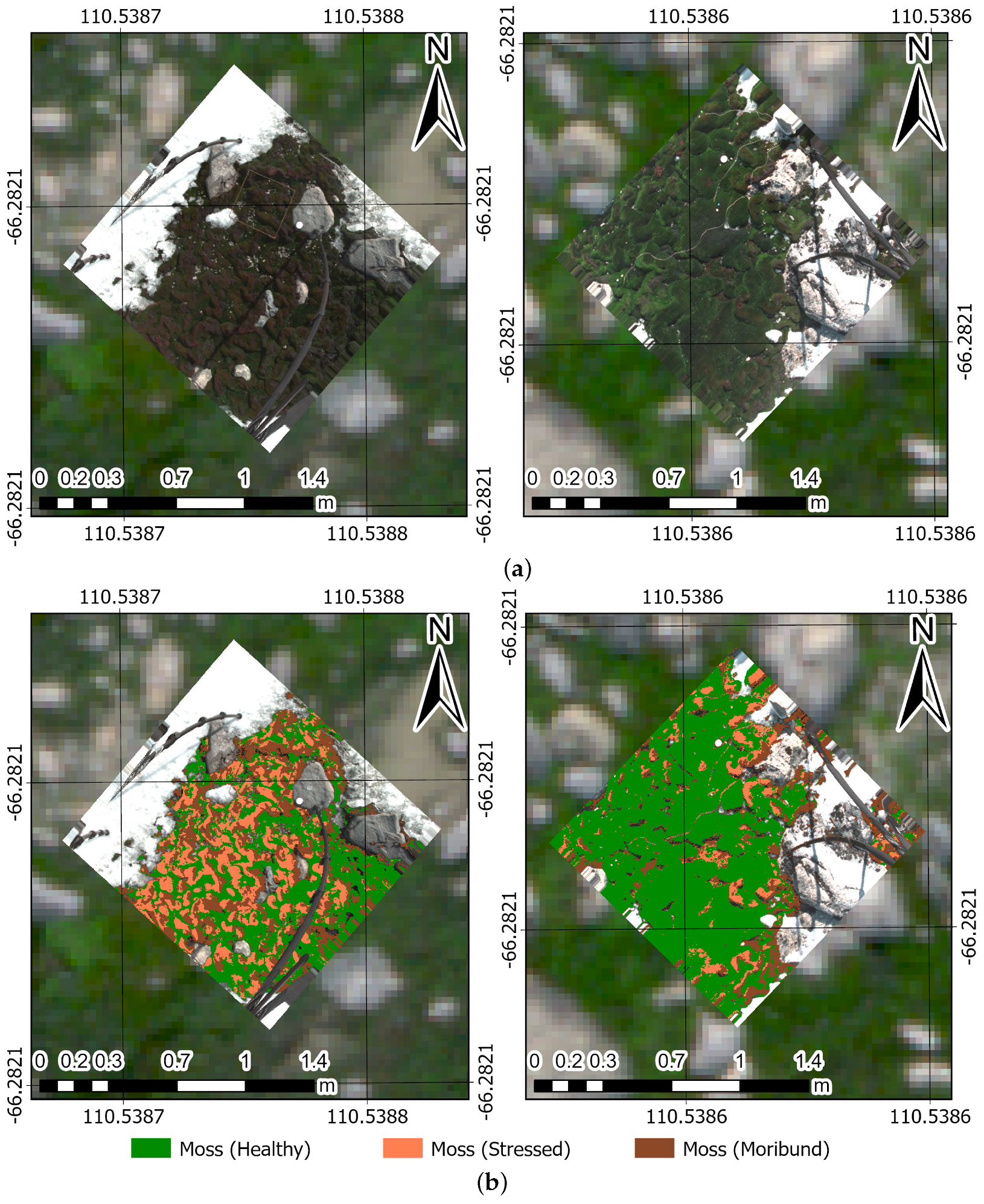
- Healthy moss: manifested by a vibrant green colour, signifying robust health.
- Moribund moss: displaying a pale-grey, brown, or black colour, signalling deteriorating health.
- Black lichen: a mix of black lichen species found at the ASPA (i.e., Usnea spp., Umbilicaria spp., and Pseudephebe spp.) and in coastal areas of the Antarctic ecosystem.
- Non-vegetated: an encompassing class that includes other materials scanned with the hyperspectral camera, such as ice, rocks, and human-made materials.
3.6. Reflectance Curves of Moss and Lichen
3.7. Spectral Indices
3.7.1. New Spectral Indices of Moss and Lichen
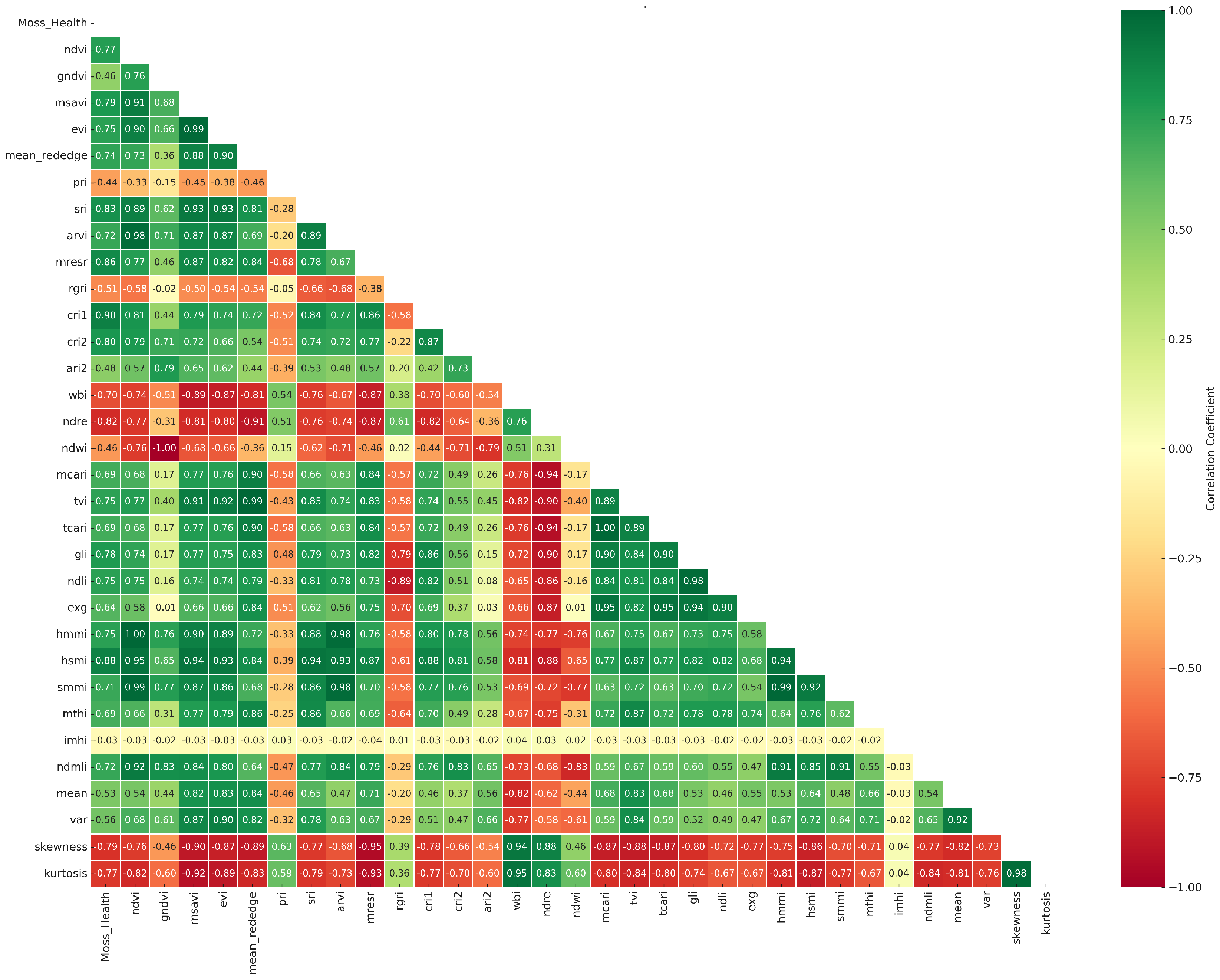
3.7.2. Correlation Matrix of Moss Health
3.8. Statistical Features
3.9. ML Classifier and Fine-Tuning
4. Results
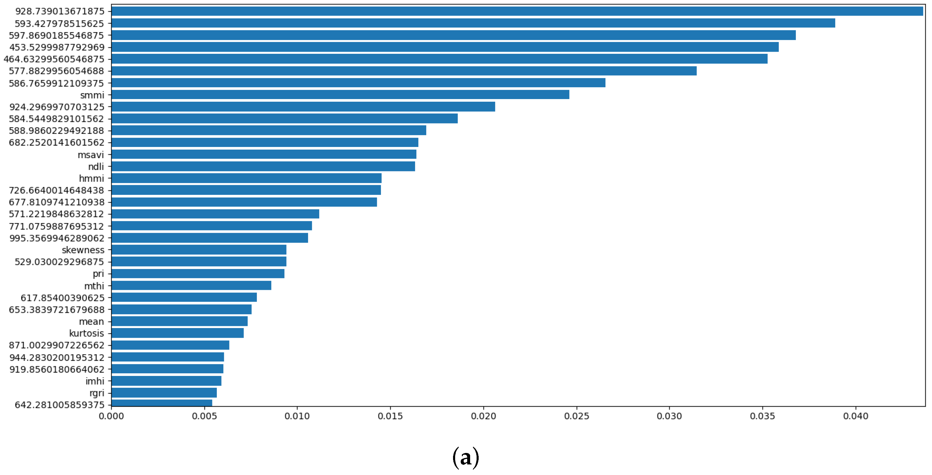
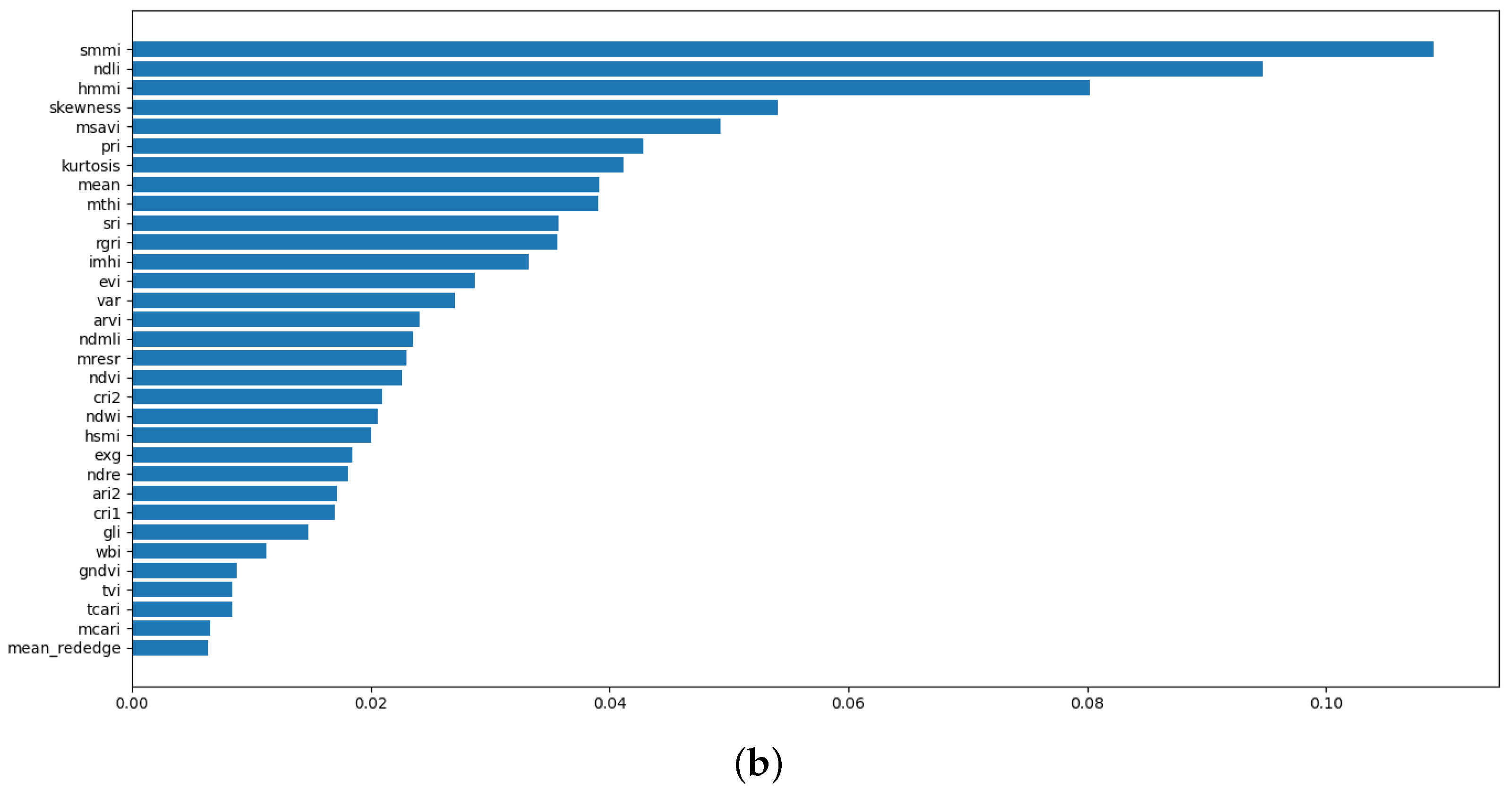
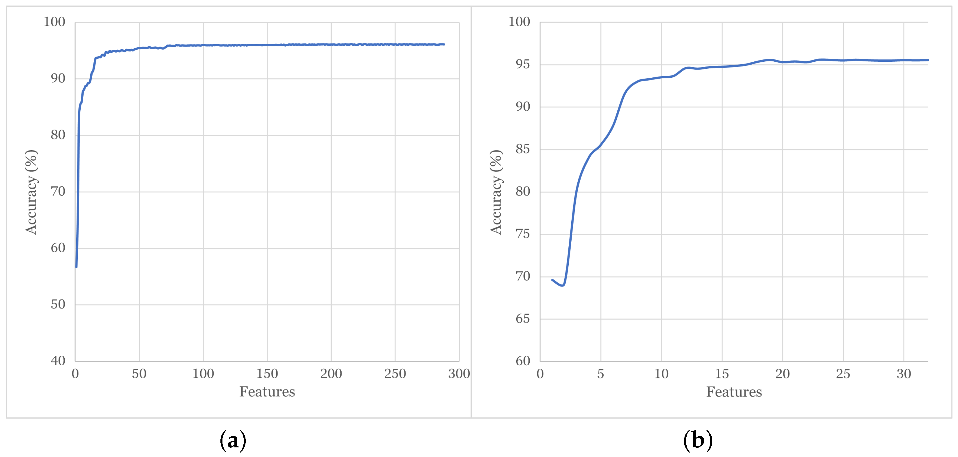
4.1. Correlation Analysis and Feature Ranking
4.2. Accuracy of Tested ML Models
4.3. Prediction Maps
5. Discussion
6. Conclusions and Future Work
Author Contributions
Funding
Data Availability Statement
Acknowledgments
Conflicts of Interest
Abbreviations
| AGL | Above-ground level |
| ASPA | Antarctic Specially Protected Area |
| DL | Deep learning |
| EVLOS | Extended visual line of sight |
| FOV | Field of view |
| GBDT | Gradient-boosted decision tree |
| GCP | Ground control point |
| GNSS | Global navigation satellite system |
| GSD | Ground sampling distance |
| HSI | Hyperspectral imagery |
| MDPI | Multidisciplinary Digital Publishing Institute |
| MP | Megapixels |
| MSI | Multispectral imagery |
| ML | Machine learning |
| NIR | Near infrared |
| RGB | Red, green, blue |
| RTK | Real-time kinematics |
| UAV | Unmanned aerial vehicle |
| XGBoost | Extreme gradient boosting |
References
- Newsham, K.K.; Davey, M.L.; Hopkins, D.W.; Dennis, P.G. Regional Diversity of Maritime Antarctic Soil Fungi and Predicted Responses of Guilds and Growth Forms to Climate Change. Front. Microbiol. 2020, 11, 615659. [Google Scholar] [CrossRef]
- Robinson, S.A.; King, D.H.; Bramley-Alves, J.; Waterman, M.J.; Ashcroft, M.B.; Wasley, J.; Turnbull, J.D.; Miller, R.E.; Ryan-Colton, E.; Benny, T.; et al. Rapid change in East Antarctic terrestrial vegetation in response to regional drying. Nat. Clim. Chang. 2018, 8, 879–884. [Google Scholar] [CrossRef]
- Yin, H.; Perera-Castro, A.V.; Randall, K.L.; Turnbull, J.D.; Waterman, M.J.; Dunn, J.; Robinson, S.A. Basking in the sun: How mosses photosynthesise and survive in Antarctica. Photosynth. Res. 2023, 158, 151–169. [Google Scholar] [CrossRef]
- Peck, L.S.; Convey, P.; Barnes, D.K.A. Environmental constraints on life histories in Antarctic ecosystems: Tempos, timings and predictability. Biol. Rev. Camb. Philos. Soc. 2006, 81, 75–109. [Google Scholar] [CrossRef]
- Bergstrom, D.M.; Wienecke, B.C.; van den Hoff, J.; Hughes, L.; Lindenmayer, D.B.; Ainsworth, T.D.; Baker, C.M.; Bland, L.; Bowman, D.M.J.S.; Brooks, S.T.; et al. Combating ecosystem collapse from the tropics to the Antarctic. Glob. Chang. Biol. 2021, 27, 1692–1703. [Google Scholar] [CrossRef]
- Convey, P.; Chown, S.L.; Clarke, A.; Barnes, D.K.A.; Bokhorst, S.; Cummings, V.; Ducklow, H.W.; Frati, F.; Green, T.G.A.; Gordon, S.; et al. The spatial structure of Antarctic biodiversity. Ecol. Monogr. 2014, 84, 203–244. [Google Scholar] [CrossRef]
- Bergstrom, D.M. Ecosystem shift after a hot event. Nat. Ecol. Evol. 2017, 1, 1226–1227. [Google Scholar] [CrossRef] [PubMed]
- Bergstrom, D.M.; Woehler, E.J.; Klekociuk, A.; Pook, M.J.; Massom, R. Extreme events as ecosystems drivers: Ecological consequences of anomalous Southern Hemisphere weather patterns during the 2001/02 austral spring-summer. Adv. Polar Sci. 2018, 29, 190–204. [Google Scholar] [CrossRef]
- Robinson, S.A.; Klekociuk, A.R.; King, D.H.; Pizarro Rojas, M.; Zúñiga, G.E.; Bergstrom, D.M. The 2019/2020 summer of Antarctic heatwaves. Glob. Chang. Biol. 2020, 26, 3178–3180. [Google Scholar] [CrossRef] [PubMed]
- Hirose, D.; Hobara, S.; Tanabe, Y.; Uchida, M.; Kudoh, S.; Osono, T. Abundance, richness, and succession of microfungi in relation to chemical changes in Antarctic moss profiles. Polar Biol. 2017, 40, 2457–2468. [Google Scholar] [CrossRef]
- Prather, H.M.; Casanova-Katny, A.; Clements, A.F.; Chmielewski, M.W.; Balkan, M.A.; Shortlidge, E.E.; Rosenstiel, T.N.; Eppley, S.M. Species-specific effects of passive warming in an Antarctic moss system. R. Soc. Open Sci. 2019, 6, 190744. [Google Scholar] [CrossRef]
- Randall, K. Of Moss and Microclimate. Spatial Variation in Microclimate of Antarctic Moss Beds: Quantification, Prediction and Importance for Moss Health and Physiology. Ph.D. Thesis, School of Biological Sciences, University of Wollongong, Wollongong, NSW, Australia, 2022. [Google Scholar]
- Newsham, K.K.; Hall, R.J.; Rolf Maslen, N. Experimental warming of bryophytes increases the population density of the nematode Plectus belgicae in maritime Antarctica. Antarct. Sci./Blackwell Sci. Publ. 2021, 33, 165–173. [Google Scholar] [CrossRef]
- Cannone, N.; Guglielmin, M. Influence of vegetation on the ground thermal regime in continental Antarctica. Geoderma 2009, 151, 215–223. [Google Scholar] [CrossRef]
- Green, T.G.A.; Sancho, L.G.; Pintado, A.; Schroeter, B. Functional and spatial pressures on terrestrial vegetation in Antarctica forced by global warming. Polar Biol. 2011, 34, 1643–1656. [Google Scholar] [CrossRef]
- Colesie, C.; Walshaw, C.V.; Sancho, L.G.; Davey, M.P.; Gray, A. Antarctica’s vegetation in a changing climate. Wiley Interdiscip. Rev. Clim. Chang. 2023, 14, e810. [Google Scholar] [CrossRef]
- King, D.H.; Wasley, J.; Ashcroft, M.B.; Ryan-Colton, E.; Lucieer, A.; Chisholm, L.A.; Robinson, S.A. Semi-Automated Analysis of Digital Photographs for Monitoring East Antarctic Vegetation. Front. Plant Sci. 2020, 11, 766. [Google Scholar] [CrossRef]
- Baker, D.J.; Dickson, C.R.; Bergstrom, D.M.; Whinam, J.; Maclean, I.M.D.; McGeoch, M.A. Evaluating models for predicting microclimates across sparsely vegetated and topographically diverse ecosystems. Divers. Distrib. 2021, 27, 2093–2103. [Google Scholar] [CrossRef]
- Malenovský, Z.; Lucieer, A.; King, D.H.; Turnbull, J.D.; Robinson, S.A. Unmanned aircraft system advances health mapping of fragile polar vegetation. Methods Ecol. Evol./Br. Ecol. Soc. 2017, 8, 1842–1857. [Google Scholar] [CrossRef]
- Turner, D.; Cimoli, E.; Lucieer, A.; Haynes, R.S.; Randall, K.; Waterman, M.J.; Lucieer, V.; Robinson, S.A. Mapping water content in drying Antarctic moss communities using UAS-borne SWIR imaging spectroscopy. Remote Sens. Ecol. Conserv. 2023. [Google Scholar] [CrossRef]
- Zhong, Y.; Wang, X.; Xu, Y.; Wang, S.; Jia, T.; Hu, X.; Zhao, J.; Wei, L.; Zhang, L. Mini-UAV-Borne Hyperspectral Remote Sensing: From Observation and Processing to Applications. IEEE Geosci. Remote Sens. Mag. 2018, 6, 46–62. [Google Scholar] [CrossRef]
- Bollard, B.; Doshi, A.; Gilbert, N.; Poirot, C.; Gillman, L. Drone technology for monitoring protected areas in remote and fragile environments. Drones 2022, 6, 42. [Google Scholar] [CrossRef]
- Bollard-Breen, B.; Brooks, J.D.; Jones, M.R.L.; Robertson, J.; Betschart, S.; Kung, O.; Craig Cary, S.; Lee, C.K.; Pointing, S.B. Application of an unmanned aerial vehicle in spatial mapping of terrestrial biology and human disturbance in the McMurdo Dry Valleys, East Antarctica. Polar Biol. 2015, 38, 573–578. [Google Scholar] [CrossRef]
- Turner, D.; Lucieer, A.; Malenovský, Z.; King, D.; Robinson, S.A. Assessment of Antarctic moss health from multi-sensor UAS imagery with Random Forest Modelling. Int. J. Appl. Earth Obs. Geoinf. 2018, 68, 168–179. [Google Scholar] [CrossRef]
- Lucieer, A.; Malenovský, Z.; Veness, T.; Wallace, L. HyperUAS-imaging spectroscopy from a multirotor unmanned aircraft system. J. Field Robot. 2014, 31, 571–590. [Google Scholar] [CrossRef]
- Chi, J.; Lee, H.; Hong, S.G.; Kim, H.C. Spectral Characteristics of the Antarctic Vegetation: A Case Study of Barton Peninsula. Remote Sens. 2021, 13, 2470. [Google Scholar] [CrossRef]
- Turner, D.J.; Malenovský, Z.; Lucieer, A.; Turnbull, J.D.; Robinson, S.A. Optimizing Spectral and Spatial Resolutions of Unmanned Aerial System Imaging Sensors for Monitoring Antarctic Vegetation. IEEE J. Sel. Top. Appl. Earth Obs. Remote Sens. 2019, 12, 3813–3825. [Google Scholar] [CrossRef]
- Turner, D.; Lucieer, A.; Malenovský, Z.; King, D.H.; Robinson, S.A. Spatial Co-Registration of Ultra-High Resolution Visible, Multispectral and Thermal Images Acquired with a Micro-UAV over Antarctic Moss Beds. Remote Sens. 2014, 6, 4003–4024. [Google Scholar] [CrossRef]
- Lucieer, A.; Turner, D.; King, D.H.; Robinson, S.A. Using an Unmanned Aerial Vehicle (UAV) to capture micro-topography of Antarctic moss beds. Int. J. Appl. Earth Obs. Geoinf. 2014, 27, 53–62. [Google Scholar] [CrossRef]
- ATS. ASPA 135: North-East Bailey Peninsula, Budd Coast, Wilkes Land. 2019. Available online: https://www.ats.aq/devph/en/apa-database/40 (accessed on 14 August 2023).
- Wasley, J.; Robinson, S.A.; Turnbull, J.D.; King, D.H.; Wanek, W.; Popp, M. Bryophyte species composition over moisture gradients in the Windmill Islands, East Antarctica: Development of a baseline for monitoring climate change impacts. Biodiversity 2012, 13, 257–264. [Google Scholar] [CrossRef]
- Australian Government. AUSPOS-Online GPS Processing Service. 2023. Available online: https://www.ga.gov.au/scientific-topics/positioning-navigation/geodesy/auspos (accessed on 27 October 2023).
- Waterman, M.J.; Bramley-Alves, J.; Miller, R.E.; Keller, P.A.; Robinson, S.A. Photoprotection enhanced by red cell wall pigments in three East Antarctic mosses. Biol. Res. 2018, 51, 49. [Google Scholar] [CrossRef]
- Waterman, M.J.; Nugraha, A.S.; Hendra, R.; Ball, G.E.; Robinson, S.A.; Keller, P.A. Antarctic Moss Biflavonoids Show High Antioxidant and Ultraviolet-Screening Activity. J. Nat. Prod. 2017, 80, 2224–2231. [Google Scholar] [CrossRef]
- Lovelock, C.E.; Robinson, S.A. Surface reflectance properties of Antarctic moss and their relationship to plant species, pigment composition and photosynthetic function. Plant Cell Environ. 2002, 25, 1239–1250. [Google Scholar] [CrossRef]
- NV5 Geospatial Solutions. ENVI|Image Processing & Analysis Software. 2023. Available online: https://www.nv5geospatialsoftware.com/Products/ENVI (accessed on 30 October 2023).
- Zeng, Y.; Hao, D.; Huete, A.; Dechant, B.; Berry, J.; Chen, J.M.; Joiner, J.; Frankenberg, C.; Bond-Lamberty, B.; Ryu, Y.; et al. Optical vegetation indices for monitoring terrestrial ecosystems globally. Nat. Rev. Earth Environ. 2022, 3, 477–493. [Google Scholar] [CrossRef]
- Rouse, J.W., Jr.; Haas, R.H.; Schell, J.A.; Deering, D.W. Monitoring Vegetation Systems in the Great Plains with ERTS; Technical Report PAPER-A20; NASA Special Publications: Washington, DC, USA, 1974.
- Gitelson, A.A.; Zur, Y.; Chivkunova, O.B.; Merzlyak, M.N. Assessing carotenoid content in plant leaves with reflectance spectroscopy. Photochem. Photobiol. 2002, 75, 272–281. [Google Scholar] [CrossRef]
- Gitelson, A.A.; Merzlyak, M.N. Remote sensing of chlorophyll concentration in higher plant leaves. Adv. Space Res. Off. J. Comm. Space Res. 1998, 22, 689–692. [Google Scholar] [CrossRef]
- Qi, J.; Chehbouni, A.; Huete, A.R.; Kerr, Y.H.; Sorooshian, S. A modified soil adjusted vegetation index. Remote Sens. Environ. 1994, 48, 119–126. [Google Scholar] [CrossRef]
- Gamon, J.A.; Serrano, L.; Surfus, J.S. The photochemical reflectance index: An optical indicator of photosynthetic radiation use efficiency across species, functional types, and nutrient levels. Oecologia 1997, 112, 492–501. [Google Scholar] [CrossRef]
- Huete, A.; Didan, K.; Miura, T.; Rodriguez, E.P.; Gao, X.; Ferreira, L.G. Overview of the radiometric and biophysical performance of the MODIS vegetation indices. Remote Sens. Environ. 2002, 83, 195–213. [Google Scholar] [CrossRef]
- Gamon, J.A.; Surfus, J.S. Assessing leaf pigment content and activity with a reflectometer. New Phytol. 1999, 143, 105–117. [Google Scholar] [CrossRef]
- Barnes, E.M.; Clarke, T.R.; Richards, S.E.; Colaizzi, P.D.; Haberland, J.; Kostrzewski, M.; Waller, P.; Choi, C.; Riley, E.; Thompson, T.; et al. Coincident detection of crop water stress, nitrogen status and canopy density using ground based multispectral data. In Proceedings of the Fifth International Conference on Precision Agriculture, Bloomington, MN, USA, 16–19 July 2000; Volume 1619, p. 6. [Google Scholar]
- Daughtry, C.S.T.; Walthall, C.L.; Kim, M.S.; De Colstoun, E.B.; McMurtrey, J.E. Estimating corn leaf chlorophyll concentration from leaf and canopy reflectance. Remote Sens. Environ. 2000, 74, 229–239. [Google Scholar] [CrossRef]
- Birth, G.S.; McVey, G.R. Measuring the color of growing turf with a reflectance spectrophotometer1. Agron. J. 1968, 60, 640–643. [Google Scholar] [CrossRef]
- Kaufman, Y.J.; Tanre, D. Atmospherically resistant vegetation index (ARVI) for EOS-MODIS. IEEE Trans. Geosci. Remote Sens. 1992, 30, 261–270. [Google Scholar] [CrossRef]
- Datt, B. A New Reflectance Index for Remote Sensing of Chlorophyll Content in Higher Plants: Tests using Eucalyptus Leaves. J. Plant Physiol. 1999, 154, 30–36. [Google Scholar] [CrossRef]
- Louhaichi, M.; Borman, M.M.; Johnson, D.E. Spatially Located Platform and Aerial Photography for Documentation of Grazing Impacts on Wheat. Geocarto Int. 2001, 16, 65–70. [Google Scholar] [CrossRef]
- Broge, N.H.; Leblanc, E. Comparing prediction power and stability of broadband and hyperspectral vegetation indices for estimation of green leaf area index and canopy chlorophyll density. Remote Sens. Environ. 2001, 76, 156–172. [Google Scholar] [CrossRef]
- Gao, B.C. Normalized difference water index for remote sensing of vegetation liquid water from space. In Proceedings of the Imaging Spectrometry, Orlando, FL, USA, 12 June 1995; SPIE: Bellingham, WA, USA, 1995; Volume 2480, pp. 225–236. [Google Scholar] [CrossRef]
- Haboudane, D.; Miller, J.R.; Pattey, E.; Zarco-Tejada, P.J.; Strachan, I.B. Hyperspectral vegetation indices and novel algorithms for predicting green LAI of crop canopies: Modeling and validation in the context of precision agriculture. Remote Sens. Environ. 2004, 90, 337–352. [Google Scholar] [CrossRef]
- Champagne, C.; Pattey, E.; Abderrazak, B.; Strachan, I.B. Mapping crop water stress: Issues of scale in the detection of plant water status using hyperspectral indices. Mes. Phys. Signatures Télédétection 2001, 79–84. [Google Scholar]
- Gitelson, A.A.; Merzlyak, M.N.; Chivkunova, O.B. Optical properties and nondestructive estimation of anthocyanin content in plant leaves. Photochem. Photobiol. 2001, 74, 38–45. [Google Scholar] [CrossRef]
- Woebbecke, D.M.; Meyer, G.E.; Von Bargen, K.; Mortensen, D.A. Color indices for weed identification under various soil, residue, and lighting conditions. Trans. ASAE Am. Soc. Agric. Eng. 1995, 38, 259–269. [Google Scholar] [CrossRef]
- The Pandas Development Team. Pandas. 2023. Available online: https://zenodo.org/records/10045529 (accessed on 28 June 2023).
- Chen, T.; Guestrin, C. XGBoost: A Scalable Tree Boosting System. In Proceedings of the 22nd ACM SIGKDD International Conference on Knowledge Discovery and Data Mining, New York, NY, USA, 13–17 August 2016; KDD ’16. pp. 785–794. [Google Scholar] [CrossRef]
- Sandino, J.; Gonzalez, F.; Mengersen, K.; Gaston, K.J. UAVs and Machine Learning Revolutionising Invasive Grass and Vegetation Surveys in Remote Arid Lands. Sensors 2018, 18, 605. [Google Scholar] [CrossRef]
- Parsons, M.; Bratanov, D.; Gaston, K.; Gonzalez, F. UAVs, Hyperspectral Remote Sensing, and Machine Learning Revolutionizing Reef Monitoring. Sensors 2018, 18, 2026. [Google Scholar] [CrossRef]
- Costello, B.; Osunkoya, O.O.; Sandino, J.; Marinic, W.; Trotter, P.; Shi, B.; Gonzalez, F.; Dhileepan, K. Detection of Parthenium weed (Parthenium hysterophorus L.) and its growth stages using artificial intelligence. Collect. FAO Agric. 2022, 12, 1838. [Google Scholar] [CrossRef]
- NVIDIA. XGBoost. 2023. Available online: https://www.nvidia.com/en-us/glossary/data-science/xgboost/ (accessed on 23 November 2023).
- Pedregosa, F.; Varoquaux, G.; Gramfort, A.; Michel, V.; Thirion, B.; Grisel, O.; Blondel, M.; Prettenhofer, P.; Weiss, R.; Dubourg, V.; et al. Scikit-learn: Machine Learning in Python. J. Mach. Learn. Res. JMLR 2011, 12, 2825–2830. [Google Scholar]
- Boggs, T. Spectral: Python Module for Hyperspectral Image Processing (0.23.1) [Computer Software]. Github. 2022. Available online: https://github.com/spectralpython/spectral (accessed on 30 October 2023).
- Harris, C.R.; Millman, K.J.; van der Walt, S.J.; Gommers, R.; Virtanen, P.; Cournapeau, D.; Wieser, E.; Taylor, J.; Berg, S.; Smith, N.J.; et al. Array programming with NumPy. Nature 2020, 585, 357–362. [Google Scholar] [CrossRef] [PubMed]
- El Mrabet, M.A.; El Makkaoui, K.; Faize, A. Supervised machine learning: A survey. In Proceedings of the 2021 4th International Conference on Advanced Communication Technologies and Networking (CommNet), Rabat, Morocco, 3–5 December 2021; pp. 1–10. [Google Scholar] [CrossRef]
- Yeturu, K. Machine learning algorithms, applications, and practices in data science. In Handbook of Statistics; Srinivasa Rao, A.S.R., Rao, C.R., Eds.; Elsevier: Amsterdam, The Netherlands, 2020; Volume 43, pp. 81–206. [Google Scholar] [CrossRef]
- Sotille, M.E.; Bremer, U.F.; Vieira, G.; Velho, L.F.; Petsch, C.; Auger, J.D.; Simões, J.C. UAV-based classification of maritime Antarctic vegetation types using GEOBIA and random forest. Ecol. Inform. 2022, 71, 101768. [Google Scholar] [CrossRef]
- Váczi, P.; Barták, M. Multispectral aerial monitoring of a patchy vegetation oasis composed of different vegetation classes. UAV-based study exploiting spectral reflectance indices. Czech Polar Rep. 2022, 12, 131–142. [Google Scholar] [CrossRef]
- Levy, J.; Craig Cary, S.; Joy, K.; Lee, C.K. Detection and community-level identification of microbial mats in the McMurdo Dry Valleys using drone-based hyperspectral reflectance imaging. Antarct. Sci./Blackwell Sci. Publ. 2020, 32, 367–381. [Google Scholar] [CrossRef]
- Kirillov, A.; Mintun, E.; Ravi, N.; Mao, H.; Rolland, C.; Gustafson, L.; Xiao, T.; Whitehead, S.; Berg, A.C.; Lo, W.Y.; et al. Segment Anything. arXiv 2023, arXiv:2304.02643. [Google Scholar]
- Hatamizadeh, A.; Yin, H.; Heinrich, G.; Kautz, J.; Molchanov, P. Global Context Vision Transformers. In Proceedings of the 40th International Conference on Machine Learning, Honolulu, HI, USA, 23–29 July 2023; Krause, A., Brunskill, E., Cho, K., Engelhardt, B., Sabato, S., Scarlett, J., Eds.; PMLR, 2023; Volume 202, pp. 12633–12646. [Google Scholar]
- Ronneberger, O.; Fischer, P.; Brox, T. U-Net: Convolutional Networks for Biomedical Image Segmentation. arXiv 2015, arXiv:1505.04597. [Google Scholar]


| Class | Name | Labelled Pixels |
|---|---|---|
| 1 | Moss (healthy) | 14,060 |
| 2 | Moss (stressed) | 12,914 |
| 3 | Moss (moribund) | 17,549 |
| 4 | Lichen (black) | 7972 |
| 5 | Non-vegetated | 56,976 |
| Total | 109,471 |
| Category | Name | Category | Name |
|---|---|---|---|
| Vegetation | Normalised Difference Vegetation Index (NDVI) [38] | Chlorophyll and Pigment | Carotenoid Reflectance Index 1 (CRI1) [39] |
| Green Normalised Difference Vegetation Index (GNDVI) [40] | Carotenoid Reflectance Index 2 (CRI2) [39] | ||
| Modified Soil Adjusted Vegetation Index (MSAVI) [41] | Photochemical Reflectance Index (PRI) [42] | ||
| Enhanced Vegetation Index (EVI) [43] | Red–Green Ratio Index (RGRI) [44] | ||
| Mean Red Edge (MRE) [45] | Modified Chlorophyll Absorption Ratio Index (MCARI) [46] | ||
| Simple Ratio Index (SRI) [47] | Stress and Disease | Atmospherically Resistant Vegetation Index (ARVI) [48] | |
| Normalised Difference Red Edge (NDRE) [45] | Modified Red-Edge Simple Ratio (MRESR) [49] | ||
| Green Leaf Index (GLI) [50] | Other | Triangular Vegetation Index (TVI) [51] | |
| Water Content | Normalised Difference Water Index (NDWI) [52] | Transformed Chlorophyll Absorption Reflectance Index (TCARI) [53] | |
| Water Band Index (WBI) [54] | Anthocyanin Reflectance Index 2 (ARI2) [55] | ||
| Excess Green (ExG) [56] |
| Name | Equation | Name | Equation |
|---|---|---|---|
| Normalized Difference Lichen Index (NDLI) | Moss Triple Health Index (MTHI) | ||
| Healthy–Moribund Moss Index (HMMI) | Inverse Moss Health Index (IMHI) | ||
| Healthy–Stressed Moss Index (HSMI) | Normalised Difference Moss–Lichen Index (NDMLI) | ||
| Stressed–Moribund Moss Index (SMMI) |
| Model | Description and Model Input | Input Features |
|---|---|---|
| 1 | A classifier incorporating over 200 reflectance bands from HSI scans, plus spectral indices, and statistical features. | 288 |
| 2 | An optimised version of Model 1, where feature selection techniques are applied to choose the best features from the original set. | 79 |
| 3 | A classifier that uses derivative features only, including spectral indices and statistical features. | 32 |
| 4 | An optimised instance of Model 3, employing feature selection to pinpoint the best derivative features for classification. | 23 |
| Class | Metric | Model 1 | Model 2 | Model 3 | Model 4 |
|---|---|---|---|---|---|
| Moss (healthy) | Precision | 0.99 | 1.00 | 0.99 | 0.99 |
| Recall | 1.00 | 1.00 | 1.00 | 0.99 | |
| F1-score | 1.00 | 1.00 | 1.00 | 0.99 | |
| Moss (stressed) | Precision | 1.00 | 0.98 | 1.00 | 0.97 |
| Recall | 0.98 | 0.99 | 0.98 | 0.98 | |
| F1-score | 0.99 | 0.98 | 0.99 | 0.98 | |
| Moss (moribund) | Precision | 0.98 | 0.96 | 0.97 | 0.94 |
| Recall | 0.98 | 0.98 | 0.98 | 0.97 | |
| F1-score | 0.98 | 0.97 | 0.98 | 0.96 | |
| Lichen (black) | Precision | 0.92 | 0.91 | 0.91 | 0.90 |
| Recall | 0.92 | 0.72 | 0.90 | 0.69 | |
| F1-score | 0.92 | 0.80 | 0.91 | 0.78 | |
| Non-vegetated | Precision | 0.99 | 0.97 | 0.99 | 0.97 |
| Recall | 0.99 | 0.98 | 0.99 | 0.98 | |
| F1-score | 0.99 | 0.98 | 0.99 | 0.97 |
| Metric | Average | Model 1 | Model 2 | Model 3 | Model 4 | Support | Class |
|---|---|---|---|---|---|---|---|
| Precision | Macro | 0.98 | 0.96 | 0.97 | 0.95 | 3322 | 1 |
| Weighted | 0.97 | 0.93 | 0.97 | 0.92 | 2485 | 2 | |
| Recall | Macro | 0.97 | 0.95 | 0.97 | 0.94 | 4405 | 3 |
| Weighted | 0.98 | 0.97 | 0.98 | 0.96 | 1465 | 4 | |
| F1-score | Macro | 0.98 | 0.97 | 0.98 | 0.96 | 15,239 | 5 |
| Weighted | 0.98 | 0.97 | 0.98 | 0.96 | |||
| Accuracy | 0.98 | 0.97 | 0.98 | 0.96 | 26,916 | Total | |
| Model | Mean Accuracy | Mean Standard Deviation |
|---|---|---|
| Model 1 | 0.95 | 0.017 |
| Model 3 | 0.95 | 0.009 |
| Class | Model | Moss (Healthy) | Moss (Stressed) | Moss (Moribund) | Lichen (Black) | Non-Vegetated |
|---|---|---|---|---|---|---|
| Moss (healthy) | 1 | 3318 | 1 | 0 | 0 | 3 |
| 2 | 3312 | 8 | 0 | 0 | 2 | |
| 3 | 3321 | 1 | 0 | 0 | 0 | |
| 4 | 3304 | 18 | 0 | 0 | 0 | |
| Moss (stressed) | 1 | 17 | 2440 | 20 | 0 | 8 |
| 2 | 14 | 2461 | 10 | 0 | 0 | |
| 3 | 16 | 2447 | 19 | 0 | 3 | |
| 4 | 24 | 2441 | 20 | 0 | 0 | |
| Moss (moribund) | 1 | 1 | 4 | 4309 | 2 | 89 |
| 2 | 2 | 47 | 4297 | 1 | 58 | |
| 3 | 1 | 6 | 4315 | 9 | 74 | |
| 4 | 3 | 50 | 4287 | 4 | 61 | |
| Lichen (black) | 1 | 0 | 0 | 20 | 1350 | 95 |
| 2 | 0 | 0 | 28 | 1048 | 389 | |
| 3 | 0 | 0 | 31 | 1325 | 109 | |
| 4 | 0 | 0 | 33 | 1011 | 421 | |
| Non-vegetated | 1 | 2 | 0 | 46 | 115 | 15,076 |
| 2 | 0 | 2 | 156 | 98 | 14,983 | |
| 3 | 1 | 0 | 68 | 125 | 15,045 | |
| 4 | 0 | 6 | 204 | 114 | 14,915 |
Disclaimer/Publisher’s Note: The statements, opinions and data contained in all publications are solely those of the individual author(s) and contributor(s) and not of MDPI and/or the editor(s). MDPI and/or the editor(s) disclaim responsibility for any injury to people or property resulting from any ideas, methods, instructions or products referred to in the content. |
© 2023 by the authors. Licensee MDPI, Basel, Switzerland. This article is an open access article distributed under the terms and conditions of the Creative Commons Attribution (CC BY) license (https://creativecommons.org/licenses/by/4.0/).
Share and Cite
Sandino, J.; Bollard, B.; Doshi, A.; Randall, K.; Barthelemy, J.; Robinson, S.A.; Gonzalez, F. A Green Fingerprint of Antarctica: Drones, Hyperspectral Imaging, and Machine Learning for Moss and Lichen Classification. Remote Sens. 2023, 15, 5658. https://doi.org/10.3390/rs15245658
Sandino J, Bollard B, Doshi A, Randall K, Barthelemy J, Robinson SA, Gonzalez F. A Green Fingerprint of Antarctica: Drones, Hyperspectral Imaging, and Machine Learning for Moss and Lichen Classification. Remote Sensing. 2023; 15(24):5658. https://doi.org/10.3390/rs15245658
Chicago/Turabian StyleSandino, Juan, Barbara Bollard, Ashray Doshi, Krystal Randall, Johan Barthelemy, Sharon A. Robinson, and Felipe Gonzalez. 2023. "A Green Fingerprint of Antarctica: Drones, Hyperspectral Imaging, and Machine Learning for Moss and Lichen Classification" Remote Sensing 15, no. 24: 5658. https://doi.org/10.3390/rs15245658
APA StyleSandino, J., Bollard, B., Doshi, A., Randall, K., Barthelemy, J., Robinson, S. A., & Gonzalez, F. (2023). A Green Fingerprint of Antarctica: Drones, Hyperspectral Imaging, and Machine Learning for Moss and Lichen Classification. Remote Sensing, 15(24), 5658. https://doi.org/10.3390/rs15245658