Machine Learning in the Hyperspectral Classification of Glycaspis brimblecombei (Hemiptera Psyllidae) Attack Severity in Eucalyptus

Abstract

Assessing different levels of red gum lerp psyllid (Glycaspis brimblecombei) can influence the hyperspectral reflectance of leaves in different ways due to changes in chlorophyll. In order to classify these levels, the use of machine learning (ML) algorithms can help process the data faster and more accurately. The objectives were: (I) to evaluate the spectral behavior of the G. brimblecombei attack levels; (II) find the most accurate ML algorithm for classifying pest attack levels; (III) find the input configuration that improves performance of the algorithms. Data were collected from a clonal eucalyptus plantation (clone AEC 0144—Eucalyptus urophilla) aged 10.3 months old. Eighty sample evaluations were carried out considering the following severity levels: control (no shells), low infestation (N1), intermediate infestation (N2), and high infestation (N3), for which leaf spectral reflectances were obtained using a spectroradiometer. The spectral range acquired by the equipment was 350 to 2500 nm. After obtaining the wavelengths, they were grouped into representative interval means in 28 bands. Data were submitted to the following ML algorithms: artificial neural networks (ANN), REPTree (DT) and J48 decision trees, random forest (RF), support vector machine (SVM), and conventional logistic regression (LR) analysis. Two input configurations were tested: using only the wavelengths (ALL) and using the spectral bands (SB) to classify the attack levels. The output variable was the severity of G. brimblecombei attack. There were differences in the hyperspectral behavior of the leaves for the different attack levels. The highest attack level shows the greatest distinction and the highest reflectance values. LR and SVM show better accuracy in classifying the severity levels of G. brimblecombei attack. For the correct classification percentage, the RL and SVM algorithms performed better, both with accuracy above 90%. Both algorithms achieved F-score values close to 0.90 and above 0.8 for Kappa. The entire spectral range guaranteed the best accuracy for both algorithms.

1. Introduction

Red gum lerp psyllid (Glycaspis brimblecombei More, 1964) is a highly invasive pest in eucalyptus plants. International agencies such as the Food and Agriculture Organization (FAO) of the United Nations have already reported concerns about this insect [1,2,3]. The adults and nymphs of the insect feed on the sap in the phloem of the plants, causing damage to the tree. In cases of severe infestation, it causes defoliation (from 20 to 30%), death of shoots and branches, and, in extreme cases, the death of some highly susceptible species, with mortality rates from 20 to 95% [1,4,5,6,7,8,9]. Lima Vieira et al. (2018) reported that leaf deformation and yellowing can also occur as a result of reduced photosynthesis caused by suction and the presence of the “shells” that protect the nymphs [10].

There may be variations in G. brimblecombei infestation between Eucalyptus species and across cultivation sites, showing that there is a certain selectivity by insects when choosing the species and its intensity of attack [11], causing different levels of damage to the plant. As a result of the damage caused to the leaves, the plant will have different spectral behavior due to the changes caused, especially to chlorophyll, structure, and internal cellular water content, making it possible to monitor or map the plant’s response to biotic stresses using sensors [12,13].

Ref. [14] carried out reflectance analyses on healthy and leafhopper-infested plants, which showed significant differences in the near-infrared (NIR) and visible (VIS) regions. Infested plants show a decrease in pigments, making it promising to use remote sensing techniques, especially those using hyperspectral sensors, to quickly map pest attack levels [15]. Ref. [16] proposed an approach using models based on deep machine learning to detect and separate plants damaged by Spodoptera frugiperda and Dichelops melacanthus in damaged and undamaged maize plants using only reflectance measurements. The authors reported that the most contributing spectral regions are located in the near-infrared range, and, to a lesser extent, in red, green, and blue, in that particular order.

Another application of these sensors is the quantification of damage levels based on mite attacks. Studies evaluating the incidence of spider mite on leaves of pepper (Capsicum annuum), common bean (Phaseolus vulgaris), and cotton using hyperspectral (400–1000 nm) and multispectral (five common bands) data, independently cross-validated by partial least squares discriminant analysis models, resulted in 100% and 95% success in identifying early damage from reflected hyperspectral data in pepper and common bean and with 92% success from multispectral data reflected in pepper. The multispectral optical sensor was also able to distinguish different levels of infestation caused by this mite at the beginning of the cotton crop cycle [17]. In this way, management decisions can be made quickly due to the availability of information [18]. Despite technological advances in agricultural practices, phenotype evaluation techniques in the field are still manual and involve less automation, being prone to being subjective [19].

Combining the use of hyperspectral data with machine learning techniques could be a promising approach to analyzing data of this nature [16]. Machine learning techniques are highly efficient when working with high-dimensional data obtained from sensors, and high classifications can be achieved even when the data may appear visually very similar [20], as can happen among healthy plants at the onset of biotic stress. The identification of isolated spectral regions is an important feature to be incorporated into studies that aim to evaluate different behaviors in plants. The main idea behind it is to propose more direct and clear spectral bands to be associated with the respective problem [16].

The evaluation of different levels of psyllid attack can influence the hyperspectral reflectance of leaves in different ways due to changes in chlorophyll. In this context, the use of machine learning can help process the data in order to classify these levels more quickly and accurately. The objectives of this study were: (I) to evaluate the spectral behavior of the levels of red gum lerp psyllid (G. brimblecombei) attack; (II) find the most accurate machine learning technique for classifying pest attack levels; (III) find the input database for the algorithms that improve their performance.

2. Material and Methods

2.1. Data Collection

Data were collected from a clonal eucalyptus plantation (clone AEC 0144—Eucalyptus urophilla), 10.3 months old, grown at a spacing of 3.0 m × 3.0 m at the experimental area of the Federal University of Mato Grosso do Sul, Chapadão do Sul Campus (coordinates 18°46′15.46″S and 52°37′26.60″W). Planting was carried out in holes with a 20 cm diameter and 60 cm depth. To improve soil fertility, the basic fertilizing consisted of 100 g of super simple, 100 g of NPK 8-28-16, and 3 g of boric acid, which were incorporated into the soil filling the hole. The experiment has 197 trees, with an average diameter at the base of the stem of 6.28 cm and average plant height of 4.83 m. Weed control was carried out by hoeing a radius of 60 cm from the seedlings and using semi-mechanized rotary cultivators between the rows.

Soil at the site is classified as red oxisol with a medium texture. According to the Köppen classification, the climate is tropical humid (Aw), with well-defined seasons, one rainy in summer and the other dry in winter, average annual rainfall of 1850 mm, and an average annual temperature ranging from 13 °C to 28 °C.

The leaves were collected between 8 and 9 a.m. from the apical third of the eucalyptus plants, randomly distributed throughout the area, avoiding borders. The leaves were stored in labeled paper containers so that the shells were not removed.

Forty eucalyptus leaves were collected for each level of G. brimblecombei infestation (Figure 1): control (no shells); N1: low infestation (average of 10 shells/leaf); N2: intermediate infestation (average of 20 shells/leaf); and N3: high infestation (average of 35 shells/leaf). The shells were quantified using a stereoscopic microscope at 40× magnification.

A total of 80 sample evaluations were carried out within each severity level, in which spectral information was obtained using a spectroradiometer (FieldSpec 3 Jr from Analytical Spectral Devices, Longmont, CO, USA). On each leaf, two readings were taken on the adaxial side in areas where there was the highest concentration of insects abaxial to the leaf. The read range is 1.4 nm in the 50 to 1050 nm range and 2 nm in the 1000 to 2500 nm range. It has a spectral resolution of 3 nm in the range from 350 to 700 nm and 30 nm in the range from 1400 to 2100 nm, obtained by means of an ASD plant probe, designed to carry out contact spectral measurements on solid materials. The equipment was calibrated using a barium sulfate white plate that reflects 100% of the light.

Once the wavelengths had been obtained, they were grouped into means of representative-band intervals as suggested by [21], in which the bands are related to important physiological processes for the plant, related to the spectral response also described by [21]. These bands are divided from B1–B28, being used as representative averages within each band: B1: 350–369; B2: 370; B3: 371–419; B4: 420; B5:421–424; B6: 425; B7: 426–444; B8: 445–475; B9: 480; B10: 481–500; B11: 501–530; B 12: 531–539; B13: 540; B14: 541–649; B15: 650; B16: 661–670; B17: 675; B18: 676–684; B 19: 685–689; B20: 690–700; B21: 701–709; B22: 710; B23: 711–730; B24: 960; B25: 1100; B26: 1400; B27: 1930; and B28: 2200.

2.2. Machine Learning Analyses

Data were submitted to ML analysis using the following algorithms: artificial neural networks (ANN), J48 decision tree (J48), REPTree (DT), random forest (RF), and support vector machine (SVM). A logistic regression (RL) analysis was used as control model. The parameters of the algorithms were set according to the default configuration of the Weka 3.8.5 software [22], except for ANN, where 10 neurons in the first layer and 10 neurons in the second layer were defined. Weka is an open-source software that brings together several machine learning algorithms for data mining tasks. It makes it possible to deal with diverse tasks with data such as classification, regression, clustering, association rule mining, and visualization.

ANN consisted of multilayer perceptron using a backpropagation algorithm with a learning rate equal to 0.3, momentum equal to 0.2, and number of epochs equal to 500. J48 is a classifier algorithm that uses an additional pruning step based on an error reduction strategy [23]. For the J48 algorithm, the parameter adopted for the minimum number of instances to allow at a leaf node was 4 and a pruning was used. REPTree (DT) is a decision tree logic that selects the best tree using information gain and performs error reduction pruning as a splitting criterion Weka’s default for the DT algorithm uses no restriction for tree depth and a minimum total weight of the instances in a leaf equal to 2.0. The RF algorithm creates several prediction trees and use a voting scheme among all learned trees to predict new values [24]. For the RF algorithm, the number of trees generated was 100, the number of execution slots to use for constructing the ensemble was equal to 1, and the remaining hyperparameters were adjusted using default settings. SVM performs classification tasks by building hyperplanes in multidimensional space to distinguish different classes [25]. SVM analysis was performed using the LibSVM Library [26] of the Weka, adopting the default setting of the software, in which the kernel type is radial basis function, the degree of the kernel is equal to 3.0, tolerance of the termination criterion (eps) is 1.0 × 10⁻⁴, and the cost parameter is equal to 1.0.

Two input configurations were tested: using only wavelengths (ALL, 350–2500 nm) and using spectral bands (SB, B1–B28), formed by the average reflectance of the spectral range of each band, totaling 28 bands, seeking to determine the input that classifies attack levels with the greater accuracy. The output variable was the severity levels of G. brimblecombei attack. Classification was carried out using stratified cross-validation with k-fold = 10 and 10 repetitions (totalizing 100 runs).

2.3. Statistical Analyses

For evaluating the classification accuracy of the algorithms, the percentage of correct classifications (CC), F-score, and kappa coefficient were estimated. Then, analysis of variance was performed, adopting a completely randomized design (CRD). For the CRD, machine learning models (ANNs, J48, REPTree, RF, and SVM) plus logistic regression (RL) applied to the two input configurations were considered. For grouping the means of CC and F-score, the Scott–Knott test at 5% probability was adopted. Afterwards, boxplot graphs were generated for the accuracy parameters (CC, F-score, and kappa) for each output variable and input configuration. Afterwards, a confusion matrix was constructed containing the correct classification values for each class on the main diagonal and the errors off the diagonal. Rbio software version 162 [27] and the ExpDes.pt and ggplot2 packages of the R software version 4.1.0 [28] were used for all statistical analyses.

3. Results

Spectral curve formed by eucalyptus leaves for each level of severity of G. brimblecombei attack were different. In the 350–700 nm range, which corresponds to the visible range (Figure 2A), there is a greater distinction between the control level and the N3 curve; the N1 and N2 curves are very close, and are similar in this range in terms of reflectance. In the 700–1300 nm range, NIR, (Figure 2B) there is a clearer distinction between the N3 and N2 curves, with a higher reflectance factor for the N3 curve. N1 and control are close and have a lower reflectance factor than the other curves.

In the 1300–2500 SWIR range, severity level N3 shows greater distinction and higher reflectance than the others. In Figure 2C, there is greater proximity between N1 and the control, while in Figure 2D, the greatest proximity is between the N2 and N1 curves. The control level shows low reflectance throughout the spectral range, while the highest severity level (N3) shows higher reflectance.

With the possibility of distinguishing the severity of the G. brimblecombei attack, data were submitted to ML analysis by means of classification. For the correct classification (CC) accuracy metric, when the input used was all the information from the spectral range evaluated, the RL and SVM algorithms achieved the best classification performance. When the input tested was SB, the RL and ANN algorithms achieved the best classification performance.

Comparing both inputs within each ANN algorithm, SB provides a better performance for this algorithm than ALL. The other algorithms perform better using ALL as an input than SB (Figure 3,

Table 1. Significant interaction for the correct classification (CC, %) accuracy metric between the machine learning (ML) algorithms and the inputs tested.

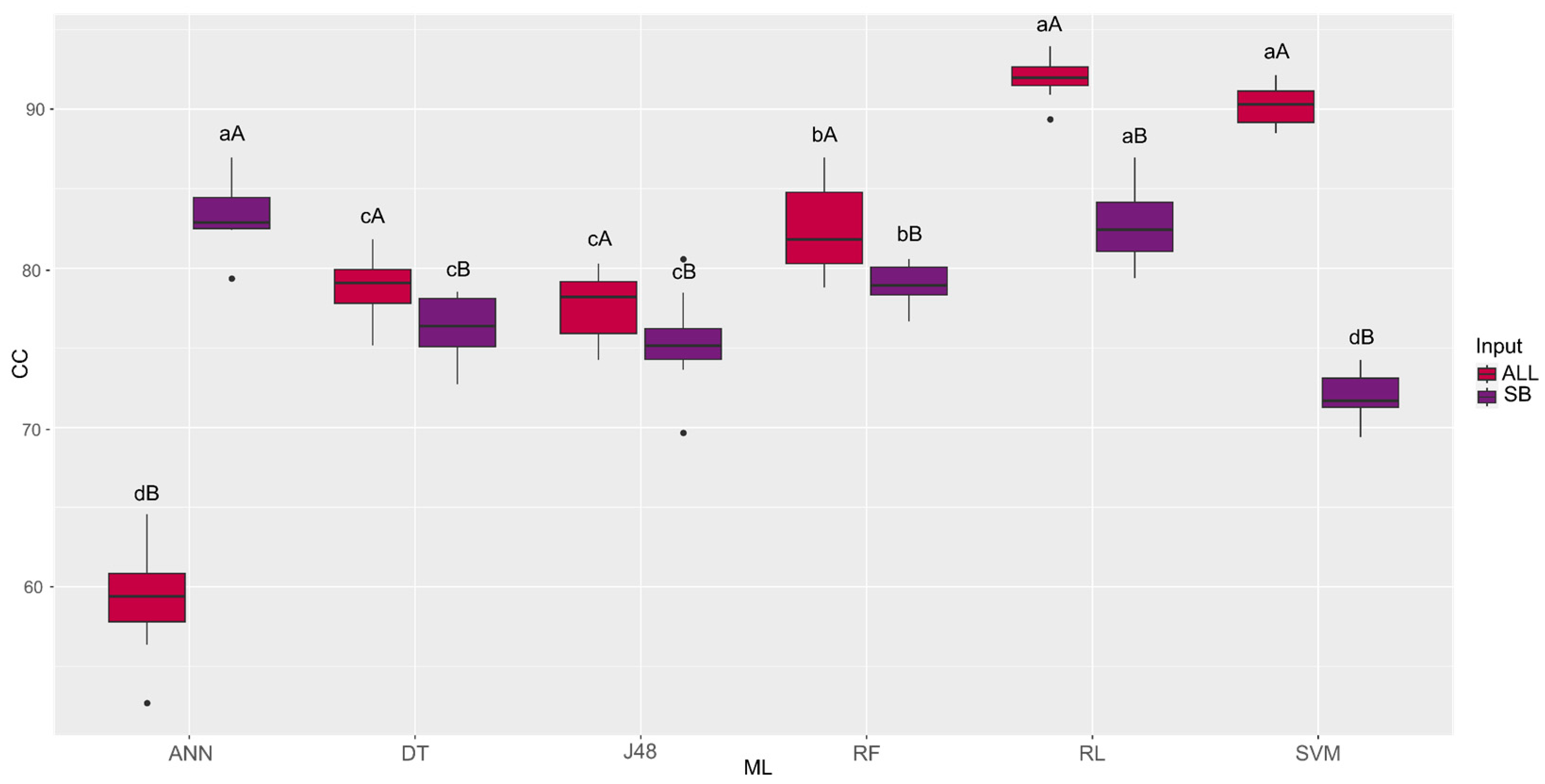
Machine Learning	ALL	SB
ANN	59.11 dB	83.38 aA
DT	78.88 cA	76.22 cB
J48	77.61 cA	75.35 cB
RF	82.38 bA	79.00 bB
RL	91.93 aA	82.69 aB
SVM	90.18 aA	72.03 dB

Means followed by the same uppercase letters in the row for the different inputs and the same lowercase letters in columns for the different ML algorithms do not differ by the Scott–Knott test at 5% probability.

).

When ALL is used as input, RL shows the best results for the F-score accuracy metric (Figure 4,

Table 2. Significant interaction for the F-score accuracy metric between the machine learning (ML) algorithms and the inputs tested.

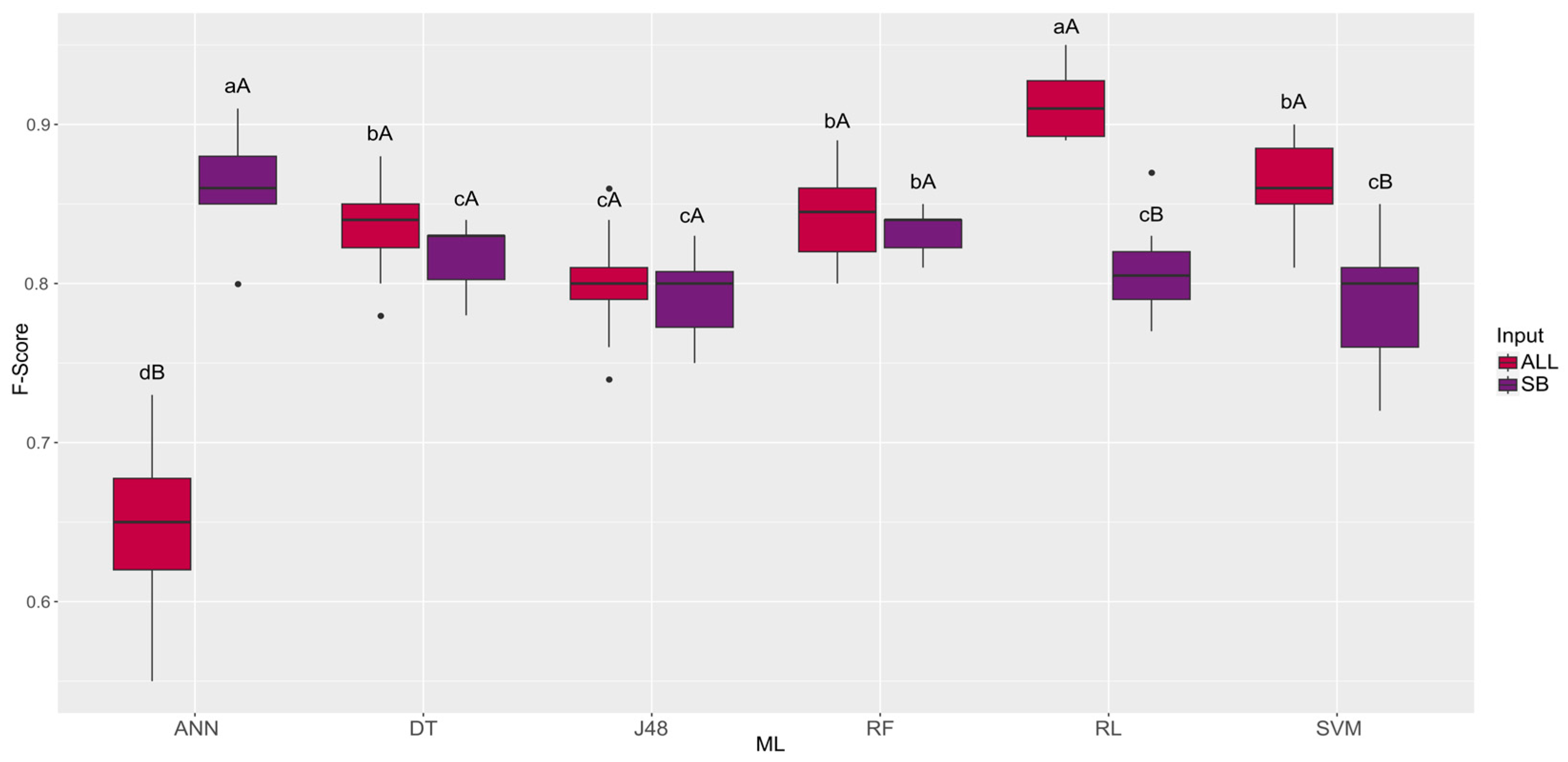
Machine Learning	ALL	SB
ANN	0.65 dB	0.86 aA
DT	0.84 bA	0.82 cA
J48	0.80 cA	0.79 cA
RF	0.84 bA	0.83 bA
RL	0.91 aA	0.81 cB
SVM	0.86 bA	0.79 cB

Means followed by the same uppercase letters in the row for the different inputs and the same lowercase letters in columns for the different ML algorithms do not differ by the Scott–Knott test at 5% probability.

). When SB is used, ANN shows better results. Comparing both inputs within each ML technique, ANN shows better accuracy than SB. DT, J48, and RF show no difference in performance between the inputs. RL and SVM show better results when the input used is ALL.

RL and SVM show better accuracy when ALL is used as input (Figure 5,

Table 3. Significant interaction for the kappa coefficient accuracy metric between the machine learning (ML) algorithms and the inputs tested.

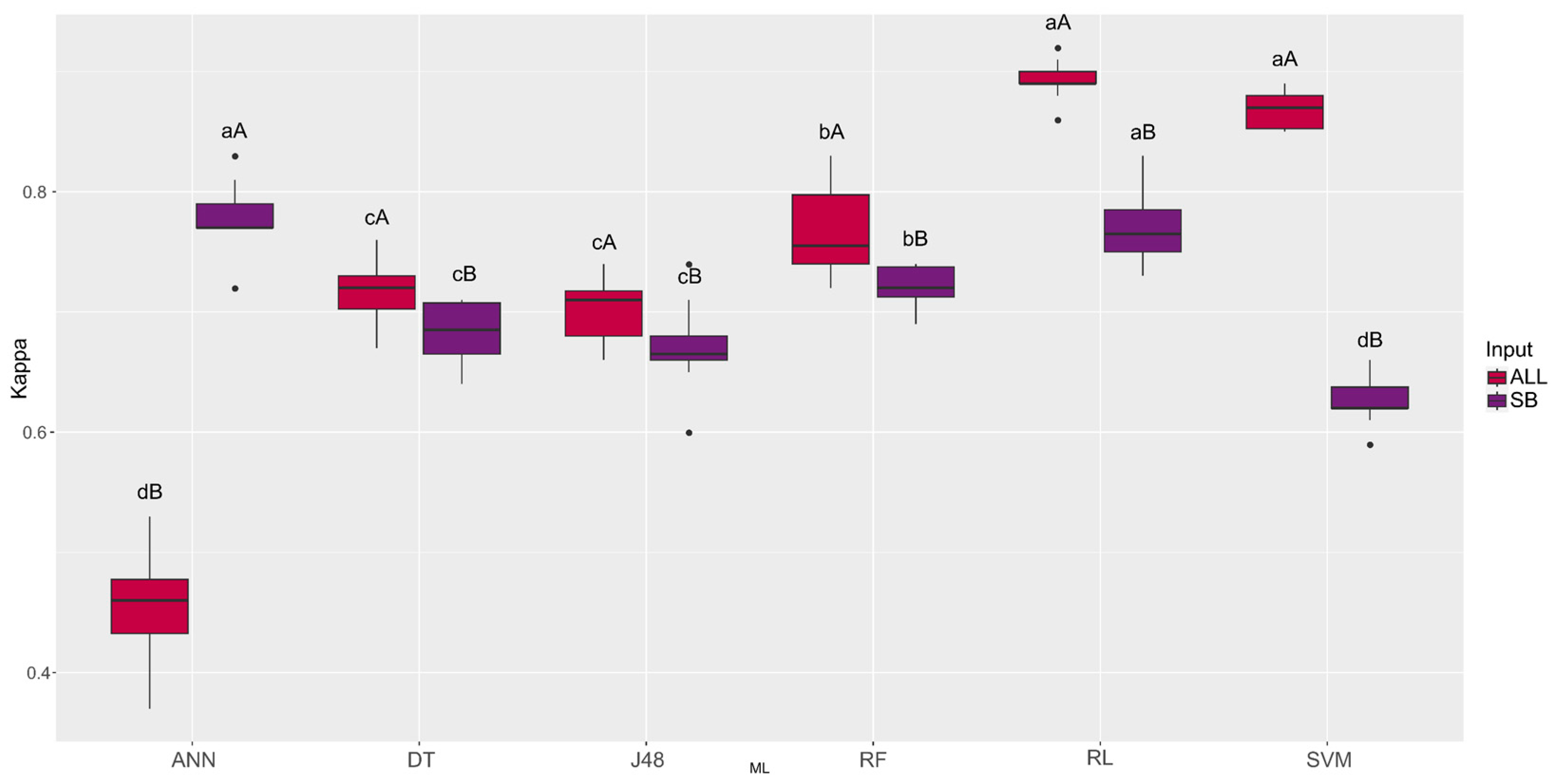
Machine Learning	ALL	SB
ANN	0.45 dB	0.78 aA
DT	0.72 cA	0.68 cB
J48	0.70 cA	0.67 cB
RF	0.77 bA	0.72 bB
RL	0.89 aA	0. 77 aB
SVM	0.87 aA	0.63 dB

Means followed by the same uppercase letters in the row for the different inputs and the same lowercase letters in columns for the different ML algorithms do not differ by the Scott–Knott test at 5% probability.

). ANN and RL show better results when SB is used as an input. When comparing the inputs within each algorithm, all algorithms except ANN perform better when ALL is used.

Overall, the RL and SVM algorithms show the best results for the three accuracy metrics tested, especially when using the ALL input, which uses all the information provided in the spectral range evaluated. Figure 6 shows the confusion matrix for the best algorithms, RL and SVM, using all the spectral information as model input. Values with dark purple shades show the number of correct classifications obtained for each cluster, while lighter pink shades show the error rate for the best configuration of each algorithm.

4. Discussion

Damage to the plant that physiologically affects chlorophyll or water content or causes cell damage interferes with the plant’s spectral response [29]. In this way, the spectral response changes according to the stress the plant is undergoing, be it from water deficit, disease, or insect attack [30]. Healthy plants reflect less in the visible range from 400 to 700 nm, due to the high absorption of these wavelengths by the photosynthesizing pigments [31]. The spectral curve of healthy leaves reflected less in this range (Figure 2A), which did not occur with plants damaged by G. brimblecombei. As the damage increased, the reflectance increased, i.e., changes in leaf reflectance caused by pest attack damage causes a decrease in photosynthesizing pigments, alters the plant’s internal water content, and damages the cell structure [12], making their leaves reflect more. Hyperspectral datasets provide particularly beneficial conditions for machine learning and deep learning due to the large amount of data, complex features, and unknown relationships [17].

When the plant suffers some stress, it is generally characterized by a higher reflectance in the visible region (400–700 nm) as a result of the lower pigment concentration [32]. It is usual that when the plant undergoes biotic stress there is a lower reflectance in the near-infrared (NIR, 700–1300 nm) and SWIR regions due to changes in the cell wall, which becomes thinner, and more air spaces occurring in the internal structure of the leaf [32]. However, each biotic stress that the plant may experience triggers different reactions, altering the color and roughness of the leaf surface in different ways, which, in turn, influences the radiation absorbed, transmitted, or reflected by it. On rough surfaces, damage causes the light beam to reflect at higher values due to the angle formed by the reflected beam at the wavelength [33], which explains the higher reflectance in the NIR band on leaves with N2 and N3 levels of G. brimblecombei infestation.

Once the reflectance of the leaves had been distinguished according to the severity level of G. brimblecombei attack, data were submitted to ML analysis in an attempt to ensure that the algorithms achieved satisfactory accuracy in distinguishing the levels. The algorithms that showed the best performance were RL and SVM using all the information in the spectral range evaluated as input. The use of ML techniques has been proposed to circumvent and solve complex issues in agriculture regarding the prediction and classification of multiple variables [34], especially when trying to relate these variables to spectral information. Furuya et al. (2021) used eight algorithms to detect attacks by S. frugiperda and D. melacanthus, with random forest (RF) performing best after the 5th day of analysis [16].

Using hyperspectral sensors can provide a large amount of relevant information across the entire spectral range, allowing for a better understanding of the features assessed [35]. Ref. [36] reported that SVM is highly effective and accurate in classifying biotic attacks on plants. Furthermore, combining spectral features with ML algorithms achieves high levels of accuracy in differentiating the different biotic attacks that plants can suffer [37]. This algorithm showed sensitivity and accuracy in detecting diseases in the early stages of attack, even without a physical signal, and its performance was increased by using hyperspectral data [38]. Additionally, reflectance values across different wavelengths guarantees more information for the algorithms, improving their performance. Hyperspectral sensing enables the detection of abiotic and biotic stresses, which opens new opportunities for pests and diseases management and field phenotyping [17].

Using all the information available from the sensor also provided better performance for algorithms such as ANN and SVM in classifying soybean genotypes for oil and protein contents in the grain [39]. Gava et al. [40], seeking to identify soybean cultivars using data from orbital sensors, achieved high accuracy using the canopy reflectance across spectral bands processed by ANN algorithm. Artificial neural networks showed good results when SB was used as an input to the algorithm. Thus, a reduced amount of information for this algorithm can provide high accuracy [38]. Powerful data manipulation and analysis approaches such as signal processing, computer vision, pattern recognition, machine learning, and data mining are associated technologies that help implement modern methods for agriculture [17].

This study brings an unprecedented and preliminary approach on the spectral behavior of eucalyptus plants under different levels of severity of G. brimblecombei infestation. This information can be used as input for training machine learning algorithms to quickly identify the start of the infestation and monitor its progress, since it has a habit of attacking the youngest leaves, which are in the outermost part of the plant canopy, associated with the size that eucalyptus can reach, which can facilitate the use of this sampling technique, and, hence, can enable the early adoption of control strategies. Such algorithms can be integrated into systems that involve the use of remote sensing, broadening the applications and benefits of this approach. This integrated framework can optimize data collection and remote analysis, making it possible to obtain accurate estimates on the severity of the infestation, providing a solid and rapid basis for decision-making, which contributes to boosting the yield of forest plantations.

5. Conclusions

The hyperspectral behavior of red gum lerp psyllid (Glycaspis brimblecombei) attack levels shows differences between healthy plants, while level one shows similar behavior. The highest attack level shows the highest and clearest difference in reflectance from the others, making it possible to distinguish the attack levels.

The logistic regression and support vector machine showed better accuracy in classifying the severity levels of G. brimblecombei attack. For the correct classification accuracy metric, the RL and SVM algorithms performed better, both with accuracy above 90. Both algorithms achieved f-score values close to 0.90 and for kappa, above 0.87–0.89. The entire spectral range guaranteed the best accuracy for both algorithms.

References

- Reguia, K.; Peris-Felipo, F.J. Glycaspis Brimblecombei Moore, 1964 (Hemiptera Psyllidae) Invasion and New Records in the Mediterranean Area. Biodivers. J. 2013, 4, 501–506. [Google Scholar]
- Ferreira-Filho, P.J.; Wilcken, C.F.; Masson, M.V.; de Souza Tavares, W.; Guerreiro, J.C.; Do Carmo, J.B.; Prado, E.P.; Zanuncio, J.C. Influence of Temperature and Rainfall on the Population Dynamics of Glycaspis Brimblecombei and Psyllaephagus Bliteus in Eucalyptus Camaldulensis Plantations. Rev. Colomb. Entomol. 2017, 43, 1–6. [Google Scholar] [CrossRef]
- Mannu, R.; Buffa, F.; Pinna, C.; Deiana, V.; Satta, A.; Floris, I. Preliminary Results on the Spatio-Temporal Variability of Glycaspis Brimblecombei (Hemiptera Psyllidae) Populations from a Three-Year Monitoring Program in Sardinia (Italy). Redia 2018, 101, 107–114. [Google Scholar] [CrossRef]
- Wylie, F.R.; Speight, M.R. Insect Pests in Tropical Forestry; CABI: Wallingford, UK, 2012; ISBN 1845936361. [Google Scholar]
- Fuentes, A.H.; Faúndez, M.; Araya, J.E. Susceptibility of Eucafyptus Spp. to an Induced Infestation of Red Gum Lerp Psyllid Glycaspis Brimblecombei Moore (Hemiptera: Psyllidae) in Santiago, Chile. Cienc. Investig. Agrar. Rev. Latinoam. Cienc. Agric. 2010, 37, 27–33. [Google Scholar]
- do Amaral Dal, M.H.F.; Wilcken, C.F.; Gimenes, M.J.; de Souza Christovam, R.; Prado, E.P. Control of Red-Gum Lerp Psyllid with Formulated Mycoinsecticides under Semi-Field Conditions. Int. J. Trop. Insect. Sci. 2011, 31, 85–91. [Google Scholar] [CrossRef]
- Wilcken, C.F.; do Couto, E.B.; Orlato, C.; Ferreira-Filho, P.J.; Firmino, D.C. Ocorrência Do Psilídeo-de-Concha (Glycaspis Brimblecombei) Em Florestas de Eucalipto No Brasil. Circ. Téc. IPEF 2003, 201, 1–11. [Google Scholar]
- Wilcken, C.F.; Firmino-Winckler, D.C.; Dal Pogetto, M.; Dias, T.K.R.; Lima, A.C.V.; de SÁ, L.A.N.; Ferreira Filho, P.J. Psilídeo-de-Concha-Do-Eucalipto, Glycaspis Brimblecombei Moore. In Pragas Introduzidas No Brasil: Insetos e Ácaros; FEALQ: Piracicaba, Brazil, 2015; pp. 883–897. [Google Scholar]
- Gill, R.J. New State Record: Redgum Lerp Psyllid, Glycaspis Brimblecombei. Calif. Plant Pest Dis. Rep. 1998, 17, 7–8. [Google Scholar]
- de Lima Vieira, R.; Pessoa, L.G.A.; de Souza Loureiro, E.; Poersh, N.L. Ocorrência de Glycaspis Brimblecombei Sobre Eucalyptus Em Chapadão Do Sul, Mato Grosso Do Sul. Rev. Agric. Neotrop. 2018, 5, 91–93. [Google Scholar] [CrossRef][Green Version]
- Jere, V.; Mhango, J.; Njera, D.; Jenya, H. Infestation of Glycaspis Brimblecombei (Hemiptera: Psyllidae) on Three Eucalyptus Species in Selected Ecological Zones in Malawi. Afr. J. Ecol. 2020, 58, 251–259. [Google Scholar] [CrossRef]
- Sankaran, S.; Mishra, A.; Ehsani, R.; Davis, C. A Review of Advanced Techniques for Detecting Plant Diseases. Comput. Electron. Agric. 2010, 72, 1–13. [Google Scholar] [CrossRef]
- Escalante-Ramirez, B. Remote Sensing-Applications; IntechOpen: Rijeka, Croatia, 2012; ISBN 9535106511. [Google Scholar]
- Pandey, P.; Prabhakar, R. An Analysis of Machine Learning Techniques (J48 & AdaBoost)-for Classification. In Proceedings of the 2016 1st India International Conference on Information Processing (IICIP), Delhi, India, 12–14 August 2016; pp. 1–6. [Google Scholar]
- Johnson, J.B.; Naiker, M. Seeing Red: A Review of the Use of near-Infrared Spectroscopy (NIRS) in Entomology. Appl. Spectrosc. Rev. 2020, 55, 810–839. [Google Scholar] [CrossRef]
- Furuya, D.E.G.; Ma, L.; Pinheiro, M.M.F.; Gomes, F.D.G.; Gonçalvez, W.N.; Junior, J.M.; de Castro Rodrigues, D.; Blassioli-Moraes, M.C.; Michereff, M.F.F.; Borges, M.; et al. Prediction of Insect-Herbivory-Damage and Insect-Type Attack in Maize Plants Using Hyperspectral Data. Int. J. Appl. Earth Obs. Geoinf. 2021, 105, 102608. [Google Scholar]
- Mahlein, A.-K.; Kuska, M.T.; Behmann, J.; Polder, G.; Walter, A. Hyperspectral Sensors and Imaging Technologies in Phytopathology: State of the Art. Annu. Rev. Phytopathol. 2018, 56, 535–558. [Google Scholar] [CrossRef] [PubMed]
- Ali, M.M.; Bachik, N.A.; Muhadi, N.; Yusof, T.N.T.; Gomes, C. Non-Destructive Techniques of Detecting Plant Diseases: A Review. Physiol. Mol. Plant Pathol. 2019, 108, 101426. [Google Scholar] [CrossRef]
- Sai Reddy, B.; Neeraja, S. Plant Leaf Disease Classification and Damage Detection System Using Deep Learning Models. Multimed. Tools Appl. 2022, 81, 24021–24040. [Google Scholar] [CrossRef]
- Adelabu, S.; Mutanga, O.; Adam, E. Evaluating the Impact of Red-Edge Band from Rapideye Image for Classifying Insect Defoliation Levels. ISPRS J. Photogramm. Remote Sens. 2014, 95, 34–41. [Google Scholar] [CrossRef]
- da Silva Junior, C.A.; Nanni, M.R.; Shakir, M.; Teodoro, P.E.; de Oliveira-Júnior, J.F.; Cezar, E.; de Gois, G.; Lima, M.; Wojciechowski, J.C.; Shiratsuchi, L.S. Soybean Varieties Discrimination Using Non-Imaging Hyperspectral Sensor. Infrared Phys. Technol. 2018, 89, 338–350. [Google Scholar] [CrossRef]
- Bouckaert, R.R.; Frank, E.; Hall, M.A.; Holmes, G.; Pfahringer, B.; Reutemann, P.; Witten, I.H. WEKA—Experiences with a Java Open-Source Project. J. Mach. Learn. Res. 2010, 11, 2533–2541. [Google Scholar]
- Al Snousy, M.B.; El-Deeb, H.M.; Badran, K.; Al Khlil, I.A. Suite of Decision Tree-Based Classification Algorithms on Cancer Gene Expression Data. Egypt. Inform. J. 2011, 12, 73–82. [Google Scholar] [CrossRef]
- Belgiu, M.; Drăguţ, L. Random Forest in Remote Sensing: A Review of Applications and Future Directions. ISPRS J. Photogramm. Remote Sens. 2016, 114, 24–31. [Google Scholar] [CrossRef]
- Rajvanshi, N.; Chowdhary, K.R. Comparison of SVM and Naïve Bayes Text Classification Algorithms Using WEKA. Int. J. Eng. Res. 2017, 6, 141–143. [Google Scholar] [CrossRef]
- Chang, C.C.; Lin, C.-J. LIBSVM: A Library for Support Vector Machines. ACM Trans. Intell. Syst. Technol. 2001, 2, 1–27. [Google Scholar] [CrossRef]
- Bhering, L.L. Rbio: A Tool for Biometric and Statistical Analysis Using the R Platform. Crop Breed. Appl. Biotechnol. 2017, 17, 187–190. [Google Scholar] [CrossRef]
- R Core Team. R: A Language and Environment for Statistical Computing; R Foundation for Statistical Computing: Vienna, Austria, 2013; pp. 275–286. [Google Scholar]
- Semeraro, T.; Mastroleo, G.; Pomes, A.; Luvisi, A.; Gissi, E.; Aretano, R. Modelling Fuzzy Combination of Remote Sensing Vegetation Index for Durum Wheat Crop Analysis. Comput. Electron. Agric. 2019, 156, 684–692. [Google Scholar] [CrossRef]
- Abdulridha, J.; Ampatzidis, Y.; Roberts, P.; Kakarla, S.C. Detecting Powdery Mildew Disease in Squash at Different Stages Using UAV-Based Hyperspectral Imaging and Artificial Intelligence. Biosyst. Eng. 2020, 197, 135–148. [Google Scholar] [CrossRef]
- Moreira, M.A. Fundamentos Do Sensoriamento Remoto e Metodologias de Aplicação, 3rd ed.; UFV: Viçosa, Brazil, 2005. [Google Scholar]
- Liu, Z.-Y.; Qi, J.-G.; Wang, N.-N.; Zhu, Z.-R.; Luo, J.; Liu, L.-J.; Tang, J.; Cheng, J.-A. Hyperspectral Discrimination of Foliar Biotic Damages in Rice Using Principal Component Analysis and Probabilistic Neural Network. Precis. Agric. 2018, 19, 973–991. [Google Scholar] [CrossRef]
- Zahir, S.A.D.M.; Omar, A.F.; Jamlos, M.F.; Azmi, M.A.M.; Muncan, J. A Review of Visible and Near-Infrared (Vis-NIR) Spectroscopy Application in Plant Stress Detection. Sens. Actuators A Phys. 2022, 338, 113468. [Google Scholar] [CrossRef]
- Christodoulou, E.; Ma, J.; Collins, G.S.; Steyerberg, E.W.; Verbakel, J.Y.; Van Calster, B. A Systematic Review Shows No Performance Benefit of Machine Learning over Logistic Regression for Clinical Prediction Models. J. Clin. Epidemiol. 2019, 110, 12–22. [Google Scholar] [CrossRef]
- Ravikanth, L.; Jayas, D.S.; White, N.D.G.; Fields, P.G.; Sun, D.-W. Extraction of Spectral Information from Hyperspectral Data and Application of Hyperspectral Imaging for Food and Agricultural Products. Food Bioprocess Technol. 2017, 10, 1–33. [Google Scholar] [CrossRef]
- Huang, L.; Liu, W.; Huang, W.; Zhao, J.; Song, F. Remote Sensing Monitoring of Winter Wheat Powdery Mildew Based on Wavelet Analysis and Support Vector Machine. Trans. Chin. Soc. Agric. Eng. 2017, 33, 188–195. [Google Scholar]
- Zhao, X.; Zhang, J.; Huang, Y.; Tian, Y.; Yuan, L. Detection and Discrimination of Disease and Insect Stress of Tea Plants Using Hyperspectral Imaging Combined with Wavelet Analysis. Comput. Electron. Agric. 2022, 193, 106717. [Google Scholar] [CrossRef]
- Khairunniza-Bejo, S.; Shahibullah, M.S.; Azmi, A.N.N.; Jahari, M. Non-Destructive Detection of Asymptomatic Ganoderma Boninense Infection of Oil Palm Seedlings Using NIR-Hyperspectral Data and Support Vector Machine. Appl. Sci. 2021, 11, 10878. [Google Scholar] [CrossRef]
- Santana, D.C.; Teodoro, L.P.R.; Baio, F.H.R.; dos Santos, R.G.; Coradi, P.C.; Biduski, B.; da Silva Junior, C.A.; Teodoro, P.E.; Shiratsuchi, L.S. Classification of Soybean Genotypes for Industrial Traits Using UAV Multispectral Imagery and Machine Learning. Remote Sens. Appl. 2023, 29, 100919. [Google Scholar] [CrossRef]
- Gava, R.; Santana, D.C.; Cotrim, M.F.; Rossi, F.S.; Teodoro, L.P.R.; da Silva Junior, C.A.; Teodoro, P.E. Soybean Cultivars Identification Using Remotely Sensed Image and Machine Learning Models. Sustainability 2022, 14, 7125. [Google Scholar] [CrossRef]