Article

A Multi-Source-Data-Assisted AUV for Path Cruising: An Energy-Efficient DDPG Approach

Division of Advanced Manufacturing, Shenzhen International Graduate School, Tsinghua University, Shenzhen 518055, China
*
Author to whom correspondence should be addressed.
Remote Sens. 2023, 15(23), 5607; https://doi.org/10.3390/rs15235607
Submission received: 6 September 2023 / Revised: 17 October 2023 / Accepted: 20 October 2023 / Published: 2 December 2023
(This article belongs to the Topic Artificial Intelligence in Navigation)

Abstract

:
As marine activities expand, deploying underwater autonomous vehicles (AUVs) becomes critical. Efficiently navigating these AUVs through intricate underwater terrains is vital. This paper proposes a sophisticated motion-planning algorithm integrating deep reinforcement learning (DRL) with an improved artificial potential field (IAPF). The algorithm incorporates remote sensing information to overcome traditional APF challenges and combines the IAPF with the traveling salesman problem for optimal path cruising. Through a combination of DRL and multi-source data optimization, the approach ensures minimal energy consumption across all target points. Inertial sensors further refine trajectory, ensuring smooth navigation and precise positioning. The comparative experiments confirm the method’s energy efficiency, trajectory refinement, and safety excellence.

1. Introduction

The marine industry has rapidly developed thanks to the increasing attention being paid to the ocean worldwide. The intricacy and unpredictability of the marine environment present substantial challenges to the effective exploitation and utilization of ocean resources. Autonomous underwater vehicles (AUVs) have emerged as invaluable assets for environmental monitoring, resource exploration, military surveillance, disaster prediction, and other critical domains due to their autonomy and mobility [1,2,3]. Many tasks require an AUV to traverse multiple essential points continuously and highly emphasize the AUV’s autonomy. A fundamental component of an AUV’s autonomy revolves around proficiently executing motion planning and obstacle avoidance [4] while concurrently managing energy consumption, which significantly influences the AUV’s application prospects.
AUV missions usually require reaching some target points, including underwater target search, underwater node maintenance, underwater information collection, etc. [5]. An AUV carries limited energy, so efficiently traversing multiple target points is vital to completing a mission. On the one hand, an AUV successfully crossing all the target points means mission completion. On the other hand, an AUV’s energy consumption is crucial because too much energy consumption may cause the AUV to fail to return, which will cause significant economic losses. These two factors determine an AUV’s success and efficiency in performing its tasks. Therefore, it is crucial to complete path cruising in the shortest cruise sequence and complete the task efficiently.
AUVs currently focus on obstacle avoidance and path planning in the execution of tasks, aiming to improve their security through algorithm innovation [6,7]. Zhu et al. [8] embedded bio-inspired neural networks into self-organizing maps to realize path planning and obstacle avoidance while ensuring comprehensive path coverage in intricate underwater environments. Hao et al. [9] introduced a motion-planning method that integrates a genetic algorithm and vector artificial potential field algorithm (VAPF). This innovative approach capitalizes on the global path-planning capabilities of the genetic algorithm and the local path-planning strengths of the VAPF to effectively address the challenges of path planning in complex and dynamically changing marine environments. Lin et al. [10] regarded the AUV flock as a whole and proposed an AUV flock control model based on an artificial potential field algorithm. This method effectively realizes the obstacle avoidance of an AUV flock in path planning. Unfortunately, the above schemes only complete the path planning but do not realize cruising to multiple target points. Motivated by AUVs needing to complete multiple tasks simultaneously, many scholars began studying AUV multi-point cruising. Yu et al. [11] combined differential evolution (DE), ant colony optimization (ACO), and clustering-based adjustment strategies to generate the DE-C-ACO algorithm, which can generate an AUV’s navigation sequence. Then, they used the shortest path faster algorithm to build the cost map between the target and candidate points. The A* search is used to complete the path planning of multiple target points. Unfortunately, it does not consider the AUV’s motion model, which makes it hardly applied. Ma et al. [12] proposed an algorithm combining velocity vector synthesis and a bionic neural network, which employs the strategy of node-space recursion and spatial decomposition to provide dynamic navigation for AUVs and uses the grid model constructed by closed boundary functions to avoid obstacles in motion forms. However, this algorithm only focuses on completing the task and does not consider the AUV’s energy consumption.
Recently, with the rapid development of computer technology, reinforcement learning has been widely used in the field of robot control [13,14] and has achieved good results by its ability to adapt to the environment. Bu et al. [15] made AUVs communicate by using sensing devices and combined the DQN algorithm with energy consumption, which weighs the information age and energy consumption to generate the optimal working path, but the obstacle avoidance ability is weakened, leading to collisions during path planning. Yang et al. [16] designed a 3D continuous motion control algorithm based on DRL and combined it with energy consumption, which maximizes the system’s energy efficiency during trajectory optimization. This method realizes multi-point communication coverage and energy optimization without fully considering the cruise sequence of target points. Considering the shortcomings of the above algorithms, this paper proposes an AUV multi-point cruising solution based on the DDPG algorithm, which combines the improved artificial potential field algorithm and the traveling salesman problem (TSP) to find the best cruise path and uses DRL to optimize the path to improve the AUV’s navigation safety and energy optimization. Specifically, the main contributions of this paper can be summarized as follows:
  • A novel approach is introduced that utilizes remote sensing data to tackle the local minima inherent in APF. This methodology is suitable for 2D and 3D environments.
  • Determining an optimal cruising sequence among multiple objectives has been likened to the traveling salesman problem (TSP). This paper proposes the TSP-IAPF method, which substitutes the Euclidean distance in the TSP with the IAPF path distance between two points. As a result, it automatically generates a cruise sequence with the shortest path across all target points.
  • This paper introduces an algorithm combining the IAPF with DDPG, integrating multi-resource data from the gyroscope, accelerometer, rangefinder, and energy consumption. By embedding this multi-source data into an IAPF-DDPG-driven motion control system, the resultant path ensures safe navigation across all target points while emphasizing energy efficiency and trajectory smoothness.
Section 2 and Section 3 present related works, motion models, and energy consumption models. Section 4 introduces the methods used, including IAPF, TSP, utilization of inertial devices, and path-planning algorithms based on DRL. Section 5 encapsulates the experimental findings, offering an intuitive illustration of the method’s superiority through comprehensive data analysis and comparisons. Section 6 shows the conclusions drawn from this study and future work.

2. Related Works

As a burgeoning type of underwater vehicle, AUVs have been widely used to perform various underwater tasks [17,18]. Guo et al. [19] used the improved genetic algorithm to optimize the navigation state and speed of the AUV execution task to save energy consumption. The method does not adequately consider the AUV’s mechanistic constraints and kinematic models. Wen et al. [20] used an ant colony algorithm and quasi-annealing algorithm to optimize the genetic algorithm, which gave AUV path planning better convergence and obstacle avoidance ability. Unfortunately, this method cannot complete the multi-target task. Yang et al. [21] embedded the enhanced dynamic window into the A* algorithm, which improved the AUV’s obstacle avoidance function and enabled the AUV to pass through multiple target points. However, this method did not consider energy consumption, making it difficult to apply to AUV tasks. Yu et al. [22] introduced a method that integrates the ant colony and A* algorithms, denoted as ACO-A*. Based on ACO path planning, the A* algorithm was used to deal with dense obstacles, realizing the purpose of completing rescue tasks in complex underwater environments. The method can perform tasks involving multiple target points but does not consider the AUV’s motion model. Sun et al. [23] proposed an AUV path coverage method based on the biomimetic neural network, which embedded discrete and centralized path planning in the biomimetic neural network to achieve the path coverage of multiple target points. This method achieves energy savings by reducing the AUV’s turn, but it does not consider the AUV’s kinematic constraints.
Recently, reinforcement learning has been widely used in AUV execution due to its excellent adaptability [24,25,26]. Zhu et al. [27] integrated sequence data into a long-short-term memory (LSTM) network and used it together with an obstacle collision prediction model (CPM) and proximal strategy optimization (PPO) network, which finally achieved a sophisticated path-planning solution for AUV navigation in dynamic underwater environments. The computational complexity of this approach is enormous due to the need to switch the memory network. This method concentrates on path planning without involving energy consumption. Chu et al. [28] introduced a path-planning methodology grounded in the double deep Q-network (DDQN). This method effectively empowers an AUV to plan paths in complex and dynamic ocean current environments by improving its neural networks and dynamic reward functions. Regretfully, this method is only suitable for a single task but cannot realize the path planning of multiple target points. Hadi et al. [29] combined the double-delay depth deterministic strategy algorithm with the navigation information of sensors in the AUV and proposed a composite reward function, and the AUV achieves nonlinear motion by controlling the fins. This method realizes AUV multi-point cruising and optimizes the AUV’s navigation control. Regrettably, this method only works for two-dimensional scenarios and does not calculate the AUV’s energy consumption. Su et al. [30] manually set multiple target points and used the double deep Q-learning network (DDQN) to proficiently execute motion-planning tasks, while the mechanical properties in the AUV are strictly limited. Energy consumption and sensor data are introduced into the algorithm, culminating in successfully completing path-planning tasks involving multiple target points with lower energy. Bu et al. [15] embedded the AUV energy consumption and communication models into the DRL to complete the underwater information acquisition task. This method uses acoustic technology to help the AUV achieve information collection, which optimizes the AUV’s energy consumption and completes multi-point cruise tasks. The AUV’s model in the above scheme is rough, and there is no index to measure energy consumption.
The work in this paper is different from the above literature. First, this paper overcomes the defect in APF by combining sensor data with TSP to produce the shortest AUV cruise sequence. Secondly, in this paper we embedded the AUV’s kinematic model, energy consumption model, and mechanical constraints into the IAPF to easily measure the AUV’s motion data. Finally, this paper combines the deep deterministic policy gradient algorithm (DDPG) and IAPF algorithm to optimize the AUV’s safety and energy consumption in the cruise path.

3. Problem Formulation

3.1. Kinematics and Dynamics Models

With limited energy, an AUV passes through multiple target points in a complex underwater environment. Finally, it reaches the designated location, which minimizes energy consumption to complete obstacle avoidance and the multi-point cruise. This is crucial in determining the AUV’s availability in the ocean. Figure 1 shows a schematic diagram where the AUV skillfully crosses multiple target points and successfully avoids obstacles to reach the target point during an underwater mission.
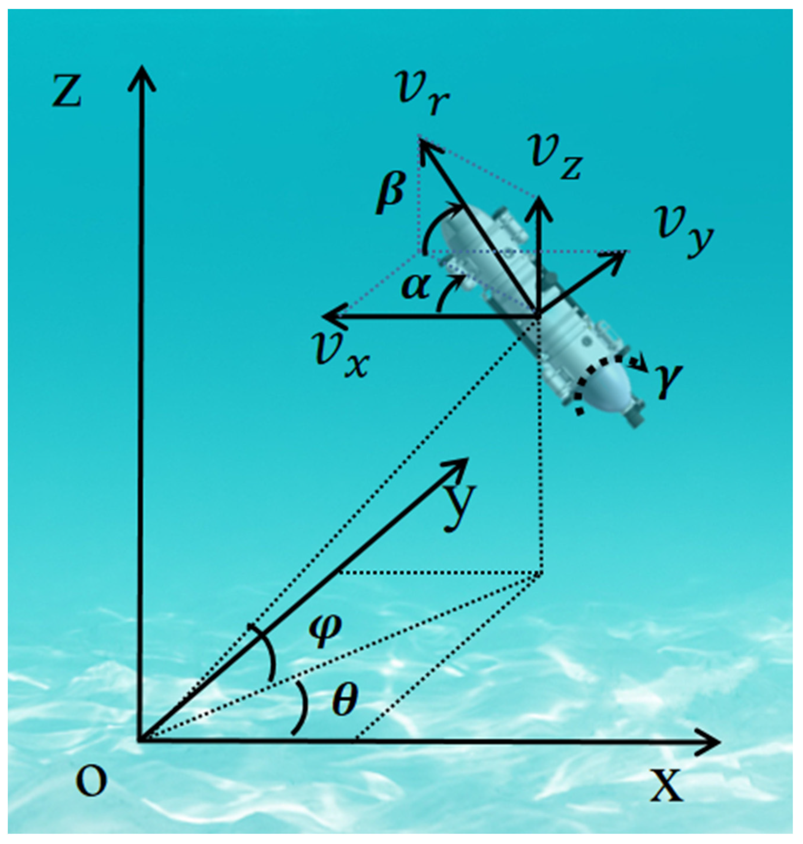
Since an AUV needs to perform tasks mainly in underwater environments, this study centers on motion planning for a three-degrees-of-freedom (3-DOFs) underdriven AUV within static settings. Figure 2 visually represents the established AUV’s kinematic and kinetic models. T.I. Fossen et al. [31] introduced the modeling approach on ships, ignoring the AUV’s swing, pitch, and rolling motion, and the models are simplified as follows:
η ˙ = R y ( α ) R z ( β ) v r ,
M v ˙ r + C ( v r ) v r + D ( v r ) v r = G ( v r ) τ ,
R y ( α ) = cos α 0 sin α 0 1 0 sin α 0 cos α ,
R z ( β ) = cos β sin β 0 sin β cos β 0 0 0 1 .
To further explain the formula, it is necessary to establish two reference coordinate systems: {a} represents the earth coordinate system, and {b} represents the body coordinate system. In Figure 2, η = [ x ,   y ,   z ] T describes the space information of the AUV within {a}. v r = [ v r ,   φ ,   θ ] T is used to represent the vector matrix, where v r is the forward velocity. φ and θ represent the pitch and yaw angles within {a}, respectively. Since the AUV’s rolling angle has no effect on navigation, γ is not taken into account in the model constraint. The navigation information within {a} is transformed into {b} through the matrix R y ( α ) and R z ( β ) . M R 3 3 denotes the mass matrix, and C ( v r ) R 3 3 signifies the Coriolis centrifugal force matrix. D ( v r ) R 3 3 designates the damping matrix, and G ( v r ) R 3 3 corresponds to the input configuration matrix. The three control signals controlling AUV’s motion are represented by τ = [ τ v ,   τ α , τ β ] T , where τ v represents the real-time forward thrust, τ α and τ β represent the real-time steering and attack angles, respectively.
The AUV’s displacement is obtained by integrating the forward velocity, and the AUV’s acceleration is obtained by differentiating the forward velocity:
L = v r d t ,
a c = v r t ,
where L represents the AUV’s displacement, and a c represents the AUV’s acceleration.

3.2. Energy Consumption Model

The AUV consumes the carried battery energy when traveling underwater. Minimizing energy consumption was achieved by analyzing the AUV’s energy consumption model and applying it to path planning. The AUV’s energy consumption power comprises two main components: propulsion power (denoted as Ρ p ) and hotel load power (denoted as Ρ h ) [32]. Ρ p is the motion-consumed power during AUV navigation, and Ρ h is the consumed power by other subsystems. Therefore, the energy consumption model can be expressed as follows:
Ρ p = ρ 2 η a η p C D A v r 3 ,
where ρ is the fluid density, C D is the drag coefficient, A is the wet surface area of the system, η a is the actuator efficiency, η p is the propulsion efficiency, and v r is the Euclidean vector norm of the velocity.
In an ideal case, the brake efficiency η a and the propulsion efficiency η p are 100%, and the formula can be simplified as:
Ρ p = ρ 2 C D A v r 3 .
This formula is the power of the AUV to overcome resistance. The velocity-varying AUV propulsion power is the sum of the resistance and speed change power. When the velocity decay is greater than the effect of drag on the AUV, the AUV does not produce the energy expenditure of the propulsion system.

4. Method

4.1. Improved Artificial Potential Field

Khatib [33] introduced a pioneering methodology known as the artificial potential field (APF) algorithm in 1986. The methodology involves manually simulating an electric potential field within the operational environment. The robot is subjected to repulsive and attractive forces within the operational environment and autonomously moves based on the integrated potential field.

4.1.1. Improved Method for Inaccessible Target

The underlying issue causing the failure to reach the target point is that the target point is not situated at a minimum point in the integrated potential field. In the APF, an additional correction factor is introduced into the repulsion potential field function to address the challenge of an inaccessible target point while keeping the attraction potential field function. This correction factor effectively balances the variations between repulsion and attraction forces, particularly when the repulsion potential field experiences rapid growth. Therefore, in the integrated potential field, while the robot approaches the target point closely, the correction factor ensures that the target point situates the minimum point. The modified repulsive function is presented as follows:
U r e p = 1 2 k r e p ( 1 ( X n X 0 ) 1 r 0 ) 2 d n ( X n , X g )     , ( X n X 0 ) r 0 0 , ( X n X 0 ) > r 0 ,
where d ( X n ,   X g ) represents the Euclidean distance between the current position and the target point, and n is a positive number. k r e p represents the repulsive factor in the repulsion potential field. From Equation (9), the repulsion potential field decreases and approaches zero while the robot approaches the target point, which guarantees the target point maintains a minimum.
The repulsion force can be derived from the revised repulsion potential field and can be represented as follows:
F r e p = U r e p = F r e p 1 + F r e p 2     , ( X n X 0 ) r 0 0 ( X n X 0 ) > r 0 ,
F r e p 1 = k r e p ( 1 ( X n X 0 ) 1 r 0 ) d n ( X n X g ) d 2 ( X n X 0 ) ,
F r e p 2 = n 2 k r e p ( 1 ( X n X 0 ) 1 r 0 ) 2 d n 1 ( X n , X g ) .

4.1.2. Improved Method for Local Minima

Ideally, the AUV will stop moving when it reaches the target point. However, while traversing an integrated potential field containing multiple obstacles, the AUV may encounter circumstances where the resulting integrated potential force becomes zero or the current position is the local minimum. In this case, the AUV will be unable to move and will not finally reach the target point. The forces on the AUV are as follows:
F = F a t t + F r e p = 0 ,
where F a t t is the attraction from the target point, and the resultant force F on the AUV is zero.
Two situations must be considered when an AUV tries to escape the “potential field trap.” First, the AUV must avoid collision with obstacles as much as possible and complete the path-planning task as soon as possible. Inspired by Zhou et al. [34], this paper invents a method to solve the “potential field trap” problem by utilizing the remote sensing data in the AUV. Remote sensing data from a sonar or photoacoustic range finder [35] are used to measure the distance continuously between the AUV and obstacles, which helps the AUV solve the local optimal problem in the APF and ensures the AUV safe navigation. The accuracy of remote sensing data is critical to ensuring the AUV’s navigation safety.
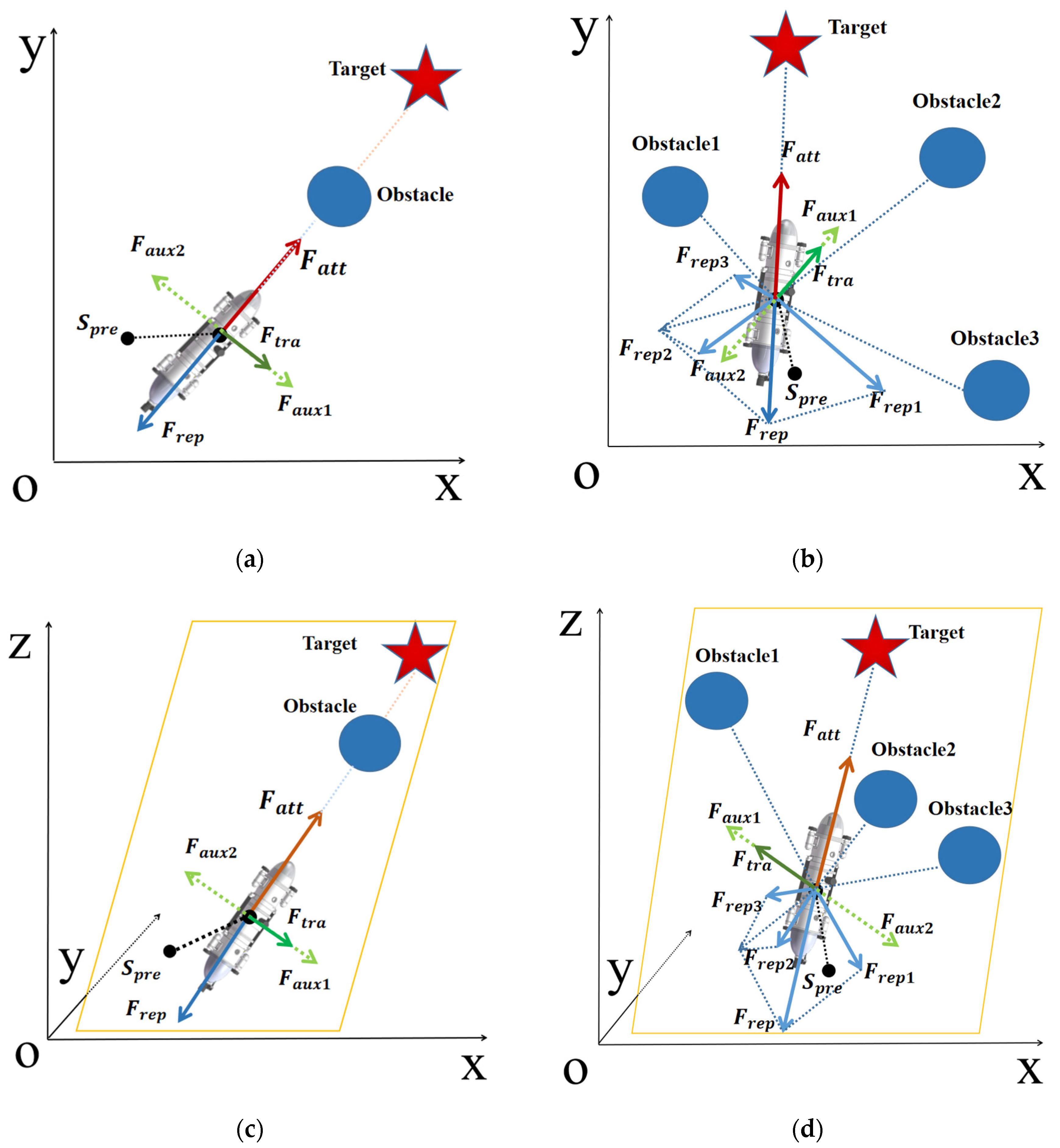
In the IAPF, the application of the AUV’s navigation includes two-dimensional (2D) and three-dimensional (3D) environments. Meanwhile, the scene is divided into a single obstacle and multiple obstacles. Figure 3 is an improvement scheme for the local optima case. The AUV trapped at a local minimum requires traction force to help it escape the trap. The auxiliary forces and traction forces required to be added to the improvement strategy are as follows:
| F a u x | = | F a t t | ,
| F t r a | = | F a u x × F r e p | ,
where the magnitude of the auxiliary force F a u x is the same as that of the attraction force F a t t , and the magnitude of the traction force F t r a is equal to that of the vector product by the auxiliary force F a u x and the repulsion force F r e p .
In the 2D environment, the scene with a single obstacle is shown in Figure 3a, and the resultant force of repulsion and attraction can be zero only if the target point, obstacle, and AUV align in a straight line. In order to get the AUV out of the local minimum, an auxiliary force needs to be constructed. Its direction should be perpendicular to the nearest obstacle for ensuring the AUV’s navigation safety. It should be at an acute angle to the previous displacement to ensure the AUV’s navigation smoothness, so it should be parallel with the F a u x 1 , and its magnitude is shown in Equation (12). The traction force is constructed from the auxiliary force. It should be in the same direction as the auxiliary force, and its magnitude is shown in Equation (13). The scene with multiple obstacles is shown in Figure 3b. Similarly, in order to ensure the AUV’s navigation safety and smoothness, the auxiliary force should be in the same direction as the F a u x 1 , and its magnitude is shown in Equation (12). The traction force is in the same direction as the auxiliary force, and its magnitude is shown in Equation (13).
In the 3D environment, the AUV trapped in the local minimum escapes the trap by constructing the auxiliary plane. The scene with a single obstacle is shown in Figure 3c, and the resultant force of repulsion and attraction can be zero only if the target point, obstacle, and AUV are aligned in the same line. The auxiliary plane is constructed by previous displacement, AUV position, and target point. In order to ensure the AUV’s navigation safety and smoothness, the auxiliary force should be in the same direction as the F a u x 1 , and its magnitude is shown in Equation (12). The traction force is in the same direction as the auxiliary force, and its magnitude is shown in Equation (13). Similarly, the scene with multiple obstacles is shown in Figure 3d, and the auxiliary plane is constructed by previous displacement, AUV position, and target point. The auxiliary and traction forces are constructed to help the AUV out of the local minimum.

4.2. Traveling Salesman Problem

The traveling salesman problem is that a businessman starting from a city wants to navigate all the target cities, and each of which must only be visited once. The problem to study is determining the most efficient path among all the feasible paths. The motion-planning problem of multi-target points is similar to that of the traveling salesman problem, finding the shortest path to cross all the points in 3D space. In multiple target tasks, it is crucial to consider obstacle avoidance and the actual path length between two points. Therefore, this paper integrates the IAPF with the TSP so that the AUV can autonomously generate a 3D path that considers the path obstacle avoidance challenges and the TSP in the underwater environment.
The mathematical expression is provided as follows:
Setting G = V ,   E as the weighted graph, V = 1 ,   2 ,   L ,   n is used for the vertex set, and E is an edge set. The distance between vertices generated using the IAPF is D i j , where D i j > 0 , and i ,   j V , and the following is set:
x i j = 1 ,                           O p t i m a l   p a t h 0 ,                                                 o t h e r       ,
So, the mathematical model of the TSP problem in 3D space is:
M i n   Z = i j D i j x i j ,
S . t   i j x i j   ,                   j V ,
i , j S x i j     k 1   ,     k V ,
x i j 0,1 ,     i V ,     j V ,
where k is all non-empty sets of V , and K is the number of all vertices of the set k , including graph G .

4.3. Utilization of Inertial Devices

There are many sensors in an AUV, such as inertial devices, and their data play a pivotal role in AUV positioning and navigation [36]. The multi-source data used in this paper include the inertial system data and the ranging system data, where the inertial system data come from the gyroscopes and the accelerometers, and they can provide real-time motion information about the AUV [37]. When an AUV is sailing underwater, it will encounter problems with speed and steering. Speed and steering angle have their threshold values, and the AUV makes it challenging to complete extreme changes. For this issue, Kalman filtering is employed for the inertial system, considering the structural and kinematic constraints specific to the AUV. Kalman filtering serves a dual purpose: it enhances AUV localization accuracy and promotes smoother motion trajectories, thus safeguarding the mechanical structure in the AUV [38].
Kalman filtering is a recursive linear quadratic estimation method for the optimal estimation of target variables by combining measurement and prediction information along with statistical noise and error information. The characteristic of its recursive processing makes it an excellent real-time property in computer applications. Kalman filtering is widely used in vehicle and aircraft navigation, signal processing, and robot control.
Kalman filtering consists of two processes: prediction and updating. During the prediction process, the current prediction value and the corresponding covariance are obtained according to the previous target value and the equation of state. Based on this, the update is combined with the measured value to obtain new target values and covariances to achieve recursion. The following are the prediction and update equations for Kalman filtering:
x k + 1 = A k x k + B k u k + w k ,
y k = H k x k + v k ,
where state x is transferred from step k to step k + 1 by a model function, x k R n represents the state space, x k denotes the measured state vector, and x k + 1 denotes the estimated state vector based on the function. A k R n n represents the transfer matrix, while u k represents the linear residual in the model. B k transforms the residual vector u k into x k . w k is set as the model estimation error. x k is linked to the observation vector y k by the observation function. H k represents the measurement matrix (ensuring the system is linear), and v k represents the measurement error.
Furthermore, assuming systematic prediction and measurement errors are Gaussian white noise, all measurements are independent. The following equation follows:
E [ v i v j T ] = r               i = j N ,
E [ w i w j T ] = Q               i = j N ,
where r is the covariance constructed by the measurement error v k , and Q is the covariance constructed by model estimation error w k .
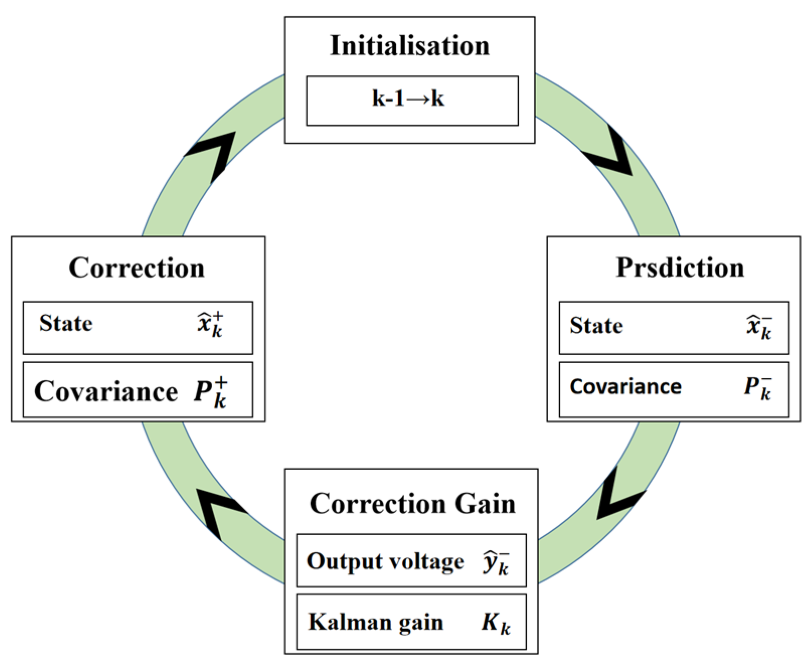
Figure 4 illustrates the Kalman filter process [39]. The Kalman filter operates as a predictor–corrector methodology. Initially, it predicts the state x ^ k and the covariance P k . Subsequently, it calculates the Kalman gain K k for this phase. Then, it corrects the prediction x ^ k + and P k + by weighting the difference between the actual measurement result u k and the predicted measurement result y k using the Kalman gain K k . Finally, this process updates x ^ k to achieve initialization.

4.4. Markov Decision Process

This paper proposes an AUV path-planning algorithm based on RL to solve the lowest energy consumption for AUV navigation trajectory while crossing multiple target points. The AUV integrates the IAPF and the TSP to derive a navigation plan that covers multiple target points with the shortest distance. Subsequently, within this navigation plan, the combination of DRL and the IAPF is employed to optimize the navigation trajectory, ultimately achieving the lowest energy consumption in the trajectory.
The path-planning problem based on RL can be formulated as a Markov decision process (MDP), represented by a five-tuple, denoted as M = S ,   A ,   P ,   R ,   γ , where S represents the state space, A represents the action space, P represents the state transition probability, R represents the reward function, and γ represents the discount factor that determines the priority of short-term rewards. At step n , given the state s S , the agent selects the action a A according to the strategy π , while receiving the corresponding reward r . When completing all actions, the total benefit is R n = i = n N γ i n r s i ,   a i , while simultaneously obtaining a series of decision trajectories τ = s 0 ,   a 0 ,   r 1 ,   s 1 ,   a 1 ,   r 2 , . . . , s T 1 ,   a T 1 ,   r T , . RL aims to find the optimal strategy that maximizes the expected cumulative reward. To apply RL to the navigation trajectory planning for the AUV, it needs to model the navigation of the AUV by MDP and then find the optimization strategy of MDP using RL. MDP is set as follows:
1.
State s n at the n step.
x n ,   y n ,   z n : 3D coordinates of the AUV in a given region.
Formally, s n = x n ,   y n ,   z n ,   D is set, where x n ,   y n ,   z n signifies the AUV’s location information, and D signifies the environmental information in space.
2.
State s n at the n step.
2.1: α ¯ n [ 0 ,   2 π ) : the steering angle of AUV at n step. β ¯ n [ 0 ,   2 π ) : the attack angle of the AUV at n step.
2.1: v ¯ n [ 0 ,   v m a x ) : the navigational velocity of the AUV at n step.
Formally, the action is defined as a n = α ¯ n ,   β ¯ n ,   v ¯ n . Since the three action variables are continuous values, trajectory optimization for the AUV constitutes a continuous control problem.
3.
Reward r n at the n step.
In the path-planning tasks, the positive reward is generally obtained only when the target point is reached, with no rewards during the movement process. Sparse rewards are generally used for path planning. In addition, at the outset of training, the agent uses a random strategy and receives the reward through a series of complex maneuvers. When the RL is directly used to optimize such problems, the training difficulty of the original algorithm will increase exponentially with the number of target points and the convergence is not guaranteed. For this issue, this paper proposes a reward-shaping mechanism that transforms the original sparse reward into a dense reward. Specifically, the reward design is defined as:
r n = r t     s m o o t h   r e w a r d r e       e n e r g y   r e w a r d r p             p a t h   r e w a r d ,
where r t is the reward at the n step, and the smoother the path, the higher the reward. r e is the energy reward at the n step, with lower energy consumption and a higher reward. r p is the path reward at the n step, and the closer to the target point, the higher the reward. The dense reward designed above allows the algorithm to converge quickly and eventually generates a path that integrates path smoothness, energy consumption, and path length.

4.5. AUV Motion-Planning Method based on DDPG Algorithm

RL, as a subfield of artificial intelligence, constructs the DRL [40]. The agent will be rewarded during training. The primary objective of RL is to maximize the total reward while the agent studies the optimal strategy to achieve predefined goals. Meanwhile, the agent refines action choices based on evaluating resulting action values during interactions with the environment. Deep learning, a pivotal part of artificial intelligence, independently learns raw data through deep neural networks and extracts high-fidelity sample features. DRL has significantly advanced continuous motion control by leveraging the strengths of both DL and RL. DDPG, as a typical DRL algorithm, has found widespread application in the transportation sector [41].

4.5.1. DDPG

Figure 5 illustrates the AUV path-planning method assisted by multi-source data and the DDPG algorithm. The actor–critic architecture, coupled with the DQN algorithm, forms the DDPG algorithm. This combination addresses the challenge of continuous action spaces while enhancing network training stability and effectiveness. Meanwhile, it solves convergence issues when approximating function values using neural networks [42]. The network structure of DDPG comprises an actor network and a critic network, each with its dedicated target and online networks. The online network is responsible for real-time action output and evaluation, as well as online parameter training and updates. In contrast, the two target networks update the value and policy network systems without conducting real-time parameter training and updates [43]. From Figure 5, the agents learn current environmental information and behavioral policy to generate appropriate actions s t . Data containing information about the current state, action, reward, and next action are then stored in an experience pool. Additionally, the neural network samples and trains the sample data in the experience pool, fine-tunes the action strategy, and makes the behavioral policy of the agent more adaptable to the environment.
Aiming at minimizing the loss function L ( θ Q ) in the critic network:
L ( θ Q ) = 1 N i ( y i Q ( s i , a i | θ Q ) ) 2 y i = r ( s i , a i ) + γ Q ( s i + 1 , μ , ( s i + 1 | θ μ ) | θ Q )   ,
where θ Q and θ Q denote the parameters in the critic network. θ μ denotes the parameter in the actor network.
The following is the actor network update policy gradient:
θ μ J = 1 N i N a i Q ( S i , a i | θ Q ) θ μ μ ( S i | θ μ ) ,
where θ μ J magnifies the policy gradient.
The weight factors are updated in the target networks as follows:
θ Q   τ θ Q + ( 1 τ ) θ Q   θ μ   τ θ μ + ( 1 τ ) θ μ   ,
where 0 τ 1 .

4.5.2. AUV Motion-Planning Model Based on DDPG Algorithm with Multi-Source Data

Figure 5 shows the multi-source-data-assisted AUV motion-planning method with multi-source data from the ranging device and the inertial sensor in the AUV. Kalman filtering is embedded in the IAPF algorithm to optimize the navigational path. The IAPF algorithm provides the DDPG with information on the AUV’s current state, including velocity, direction, angular speed, environmental obstacles, and the target point. The energy consumption model is embedded into the reward function, and the DDPG algorithm generates the optimal action output based on the AUV’s state information and the reward function. The action output is converted into six-degrees-of-freedom data in the Cartesian coordinate system. The data information is stored in the experience pool and randomly sampled for training. Simultaneously, the AUV continuously learns from these actions, improving subsequent control policy. Finally, the model with the highest cumulative reward is selected from all the models as the training model for the AUV and generates the cruise path. For the DDPG model, in the critic network, two hidden layers have 512 and 256 neurons, respectively. In the actor network, both hidden layers have 256 neurons. The hidden layers employ the ReLU activation function, while the final layer utilizes the Tanh activation function, constraining the output value between -1 and 1.

4.5.3. State Space

In the DDPG framework, the AUV gathers valuable information from the state space and leverages it to optimize its decision. In this experiment, as input to the neural network, the state space is configured as:
S t = [ x t ,   y t ,   z t ,   D ] ,
where [ x t ,   y t ,   z t ] denotes the position information within Cartesian coordinate space, and D corresponds to the environment information.

4.5.4. Action Space

The motion of the AUV is 3-DOFs, including the yaw angle, pitch angle, and velocity:
a t = [ v t , α t , β t ] ,
where v t is the velocity. α t and β t are the yaw and attack angles, respectively.

4.5.5. Reward Function

The reward function is a critical element for algorithm convergence and plays a central role in accomplishing the navigation task. The common sparse rewards do not converge well in path planning with multiple objectives, so this paper uses dense rewards. This paper adopts the following reward function:
r e w a r d = + 10 R e a c h   t a r g e t   p o i n t 30 H i t   t h e   o b s t a c l e d i s 1 d i s 2 0.01 v 3 0.1 ( α + β ) t h e   n   s t e p ,
where d i s 1 is the distance from the current position to the target point, and d i s 2 is the distance from the starting point to the target point. v is the velocity at the n step, α is the steering angle at the n step, and β is the attack angle at the n step. Using the above dense rewards, the AUV can reduce energy consumption and keep the path smooth while completing the path planning.

4.5.6. Mixed Noise

The robot’s search capability is improved since the DDPG output action includes noise. The two common types of noise used are Gaussian noise and OU noise. Gaussian noise generates uncorrelated perturbations in time series, while OU noise generates correlated perturbations. OU noise has the property that the previous step influences the current step, and it is calculated using the following formula:
N O U ( d a t ) = θ ( a ¯ a t ) d t + δ d W t ,
where a t represents the action at time t , θ represents the learning rate in the random process, a ¯ represents the average of the action sampling data, δ represents the random weights of OU, and W t represents the Wiener process.
Mixed noise can further enhance the optimization of the search strategy, so the mixed noise composed of Gaussian noise and OU noise in this paper is as follows:
a t N G a u s s i a n ( a t + N O U ( d a t ) , v a r ) ,
where v a r denotes the Gaussian variance. As the robot accumulates training experience and adapts to the environment, it becomes necessary to reduce the search rate. Thus, v a r is defined as v a r = v a r C , and C is the specified decay rate.
The motion-planning method for multiple target points proposed in this paper addresses improving the APF algorithm, integrating DRL, and incorporating multi-source data into path planning to make the generated paths safer and to lower energy consumption. The quasi-code of the DDPG algorithm-based multi-source-data-assisted AUV for path cruising with multiple target points is as follows (Algorithm 1):
Algorithm 1. Multi-source-data-assisted AUV for path cruising based on the DDPG algorithm.
Remotesensing 15 05607 i001

5. Simulation Results

This paper introduces a novel approach to improve APF, suitable for 2D and 3D environments. Since the improved principle for APF in 2D and 3D environments is the same, and the 3D environment contains the 2D environment, only the 3D environment is required in the simulation. In this paper, we adopt the learning framework of DDPG and set up a simulation environment for 11 * 12 * 6 hm with multiple obstacles, while embedding both the motion and the energy models into the AUV. This simulation environment is built on a fixed inertial coordinate system, and the AUV is cruising in that coordinate system, which is a linear system. Information related to location variations is based on this coordinate system. Alternatively, the information related to navigation angle is based on the fixed body coordinate system in the AUV. The information in the fixed body coordinate system is converted into that in the fixed ground coordinate system by matrix calculation. In the simulation, the AUV moves using equal time intervals so that location variations, velocity, and acceleration can be transformed into each other and directly limit each other. The algorithm is trained a thousand times to obtain the best-trained model, which is used to generate the optimal cruise path. The comparison experiments used advanced reinforcement learning algorithms including PPO and TD3. The simulation experiment mainly includes multiple cruising target points and tracking performance under the remote sensing error for the AUV. The following conventions display data conveniently: positive values for left turns, negative values for right turns, positive values for climb angles, and negative values for descent angles. Table 1 shows the mechanical capacity parameters for the AUV and the hyperparameters for DDPG.

5.1. Target Point Cruise Sequence

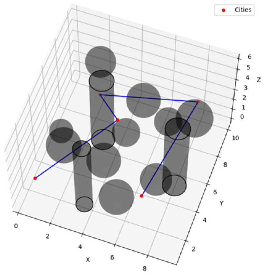
The start and target points were randomly set, and the cruise sequence for the target points was automatically generated using the proposed TSP-IAPF method. In the obstacle environment, IAPF is used for path planning and to generate the corresponding path distance between different points. Then, the path distance is introduced into the TSP problem, which generates the cruise sequence for multiple target points with the shortest path. Several target points are randomly selected in the simulation environment, and the cruise sequence pathways randomly generated according to the TSP-IAPF method are shown in Figure 6. The cruise sequence can be clearly seen in the figure, and the subsequent comparison experiment will continue and simulate according to it.

5.2. Motion Planning for Multiple Target Points

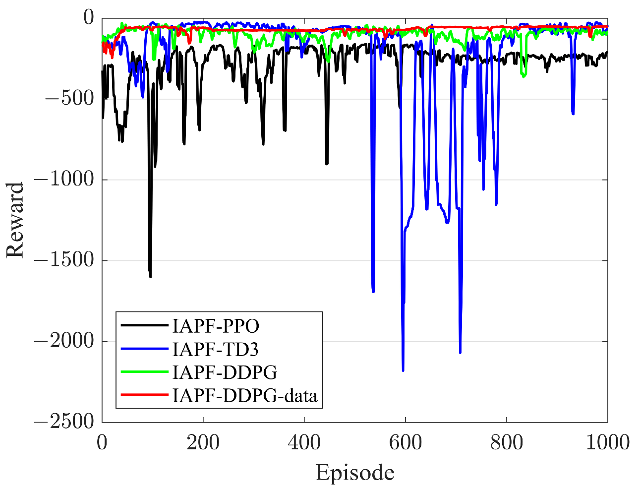
The comparison algorithm adopts the RL methods to better show the motion-planning effect of the proposed algorithm. The algorithms in the comparison experiments are TD3-IAPF, PPO-IAPF, DDPG-IAPF, and DDPG-IAPF-data. Figure 7 displays the reward curves of these four algorithms, with clear evidence that the proposed algorithm achieves rapid convergence.
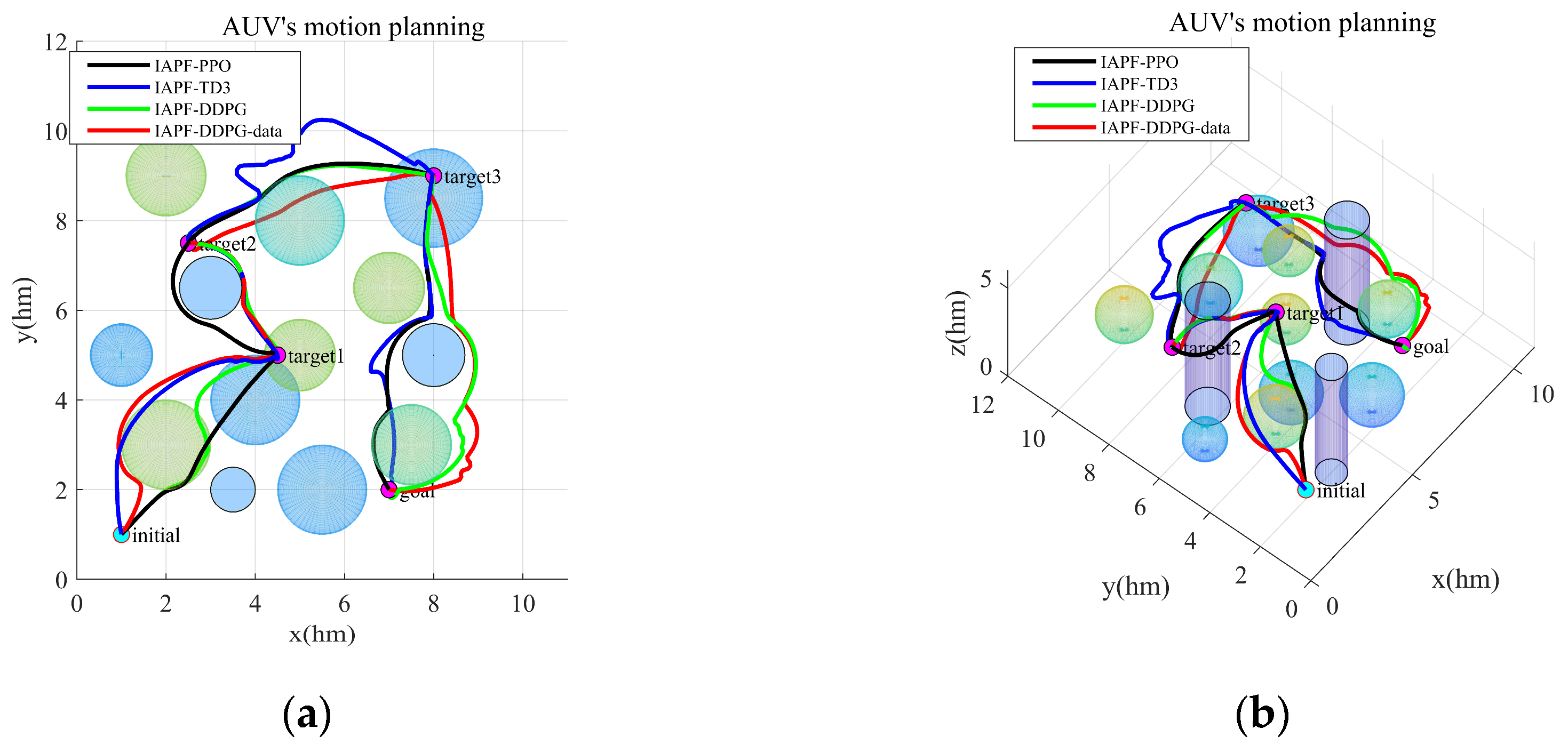
Figure 8 depicts the 3D paths of motion planning generated by the four algorithms, with Figure 8a showing the top view and Figure 8b showing the 3D view. In Figure 8, the AUV crosses four target points in turn, and the black, blue, green, and red curves are motion-planning curves generated by the four algorithms, respectively. It becomes evident that the red and black curves are relatively smooth, while the blue and the green curves have more turning line segments. To clearly show the data for the AUV in motion, this paper exports the data during the movement-planning process and draws data including pitch angle, the closest distance to an obstacle (collision uses negative value), attack angle, steering angle, speed, and acceleration. Figure 9 shows the curves of the above data.
Figure 9 illustrates various motion data related to the AUV and generated by the four algorithms. The attack angle signifies the vertical plane’s angle between the previous and current steps’ displacement, while the steering angle signifies the horizontal plane’s angle between these displacements. Figure 9a shows the data about steering angle, Figure 9b shows the data about attack angle, Figure 9c shows the data about pitch angle, Figure 9d shows the data about the closest distance to the obstacle, Figure 9e shows the data about velocity, and Figure 9f shows the data about acceleration. According to Figure 9a,b, it can be clearly concluded that the turn of the AUV in underwater navigation is optimized, and the occurrence of extreme turns is reduced, which facilitates easier steering and safeguards the AUV’s mechanical structure. The pitch angle represents the AUV’s forward posture while sailing, and it can be seen from Figure 9c that the posture while moving forward has been improved. Figure 9d highlights that the proposed algorithm ensures that the AUV maintains a safer distance from underwater obstacles when navigating underwater. The superiority of the method proposed in this paper can be directly shown by comparing it with other algorithms. Figure 9e indicates the velocity data of the AUV, and Figure 9f demonstrates the acceleration data of the AUV. Figure 9e,f indicate that the proposed algorithm excels in velocity and acceleration control. Figure 9 clearly demonstrates that the proposed algorithm has smooth turn advantages, safety and reliability, and velocity control.
For a concise comparison, the motion data in the experiment are displayed in Table 2, including energy consumption, average steering angle, average attack angle, pitch angle, closest distance to the obstacle, velocity, acceleration, path length, and navigation time. Combining the data presented in Figure 9 with the information in Table 2, it becomes evident that the proposed algorithm achieves multi-target point cruising tasks with reduced energy consumption while ensuring safe navigation. Meanwhile, the planned motion trajectory has less steering, which makes turning for the AUV easier to achieve.
This paper uses Monte Carlo experiments to test the reliability of the four algorithms. For facilitating the comparison of experimental results, a predefined number of obstacles were selected in a static obstacle environment and were set to change positions randomly, and 500 simulations were performed. Figure 10 illustrates the experimental outcomes visually. Figure 10a shows the energy consumption and the closest distance to the obstacle for the AUV, and Figure 10b shows the travel time and path length for the AUV. Figure 10a shows that the proposed algorithm excels in ensuring safe navigation and minimizing energy consumption. It can be observed from Figure 10b that the proposed algorithm possesses better path stability when the environment changes. Based on the results from the Monte Carlo experiments, the proposed algorithm has excellent performance in terms of safety, energy consumption, and path stability during motion planning.
This study conducts simulations for dynamic underwater environments to better adapt to realistic underwater navigation scenarios. This simulation environment is built on a fixed inertial coordinate system, wherein static obstacles remain stationary while dynamic obstacles undergo linear motion. For a concise comparison, the obstacle positions in the static environment are simply adjusted so that none of the paths generated by the four algorithms collide, and then the dynamic obstacles are added. Figure 11 shows the motion-planning curves generated by the four algorithms in the dynamic environment, and the AUV’s motion data in the dynamic environment are extracted and presented in Table 2.
It is obvious from Figure 11 that the IAPF-PPO algorithm and the IAPF-DDPG-data algorithm have fewer turns in the path profile for motion planning. Combining the data in Table 3, it becomes evident that the proposed algorithm has obvious advantages in navigation safety. Additionally, the algorithm displays strong performance in energy consumption and turning control. It is illustrated that embedding multi-source data into the DRL algorithm and using the algorithm to assist the AUV in motion planning have more significant potential.

5.3. Trajectory Tracking and Path Optimization with Remote Sensing Information

The AUV must follow a pre-designed route when performing path cruising with multiple target points. The remote sensing equipment’s performance differences and detection errors caused the AUV to deviate from its intended cruise path when navigating underwater. Consequently, this research emphasizes the trajectory-tracking task under detection errors and the impact of remote sensing equipment performance differences on energy consumption and navigation safety.
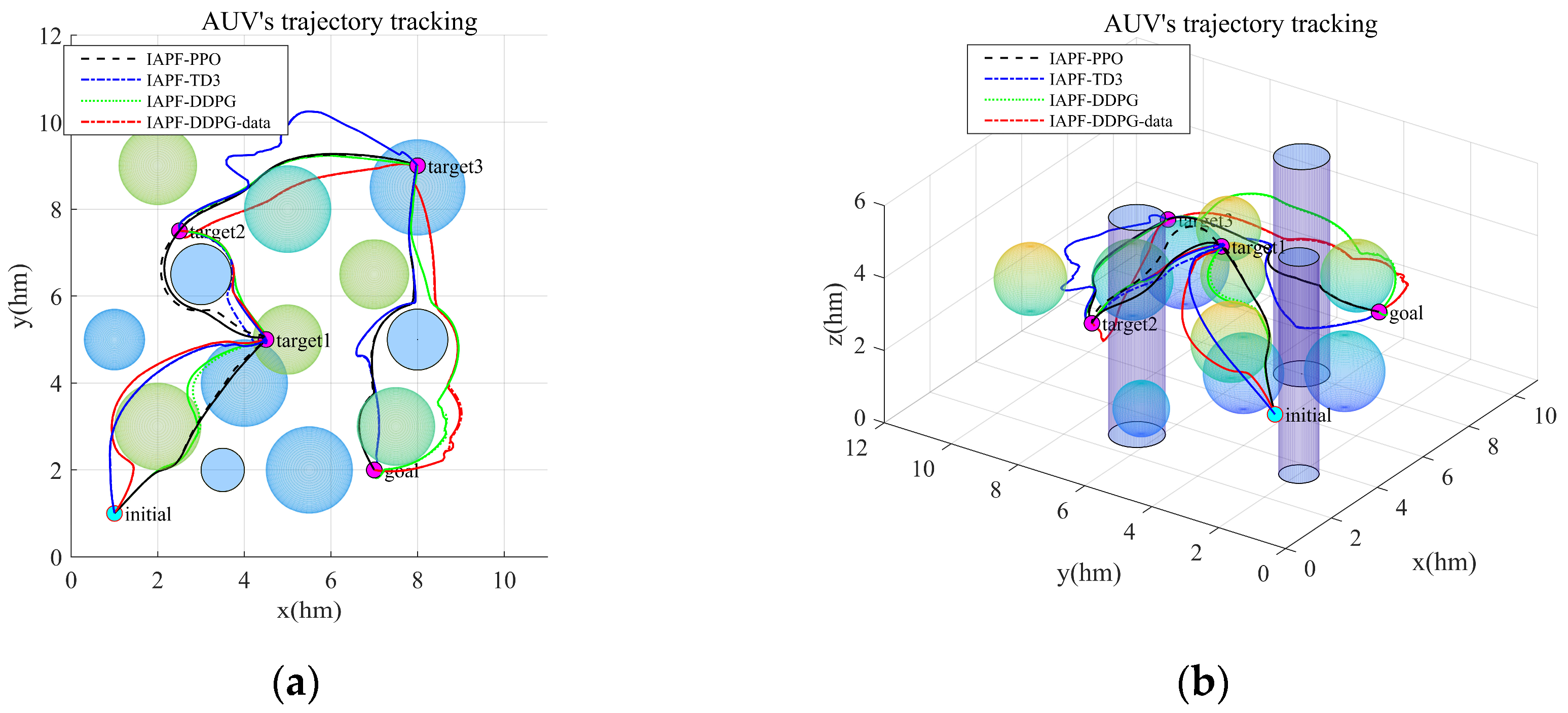
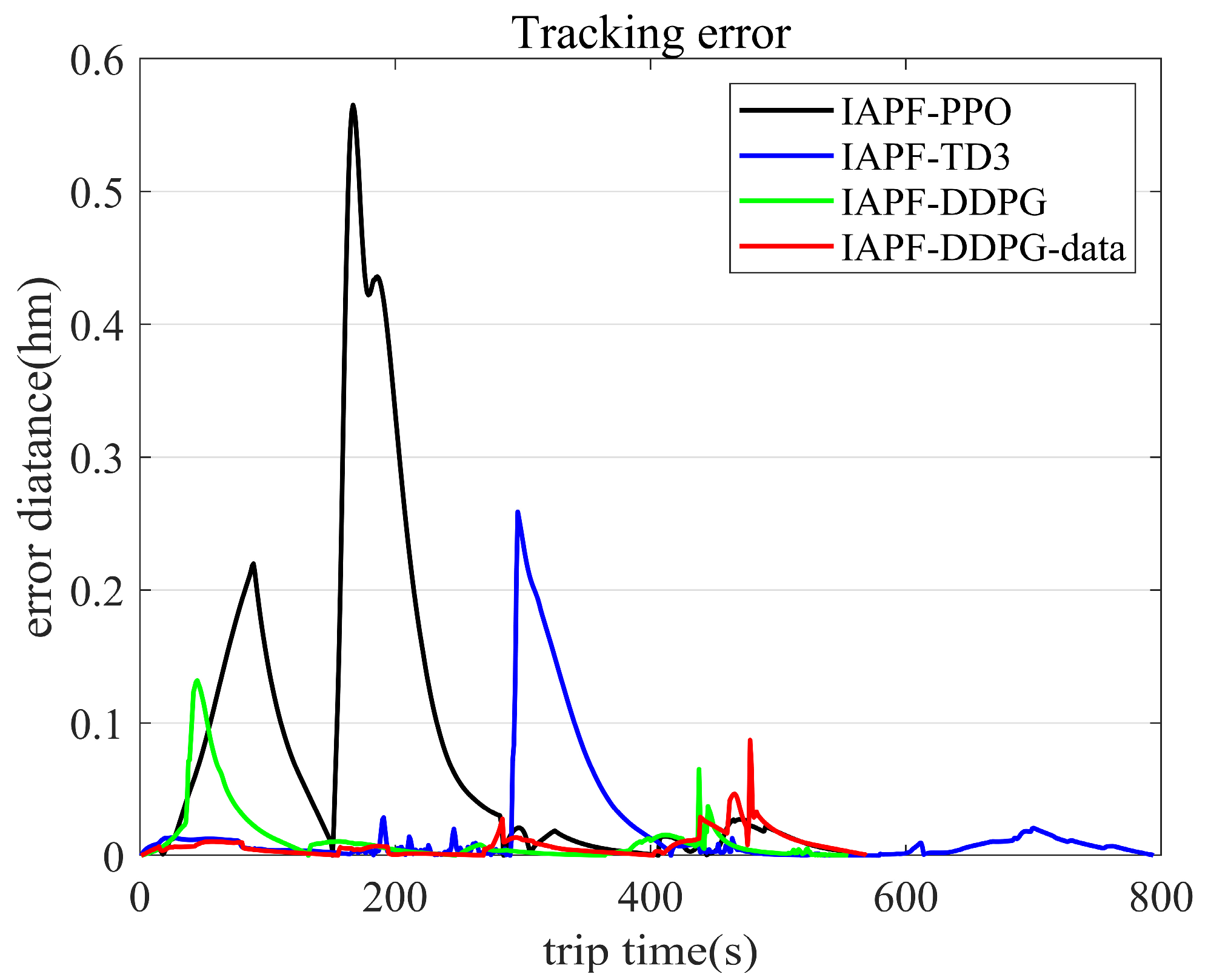
Since the accuracy of the underwater detection equipment is above one percent, this experiment sets the detection error to one percent. It explores the AUV’s trajectory-tracking capability in a static environment. Figure 12 shows that the AUV’s movement under the detection error.
During the trajectory tracking, the AUV’s main task is to avoid collision. For showing the tracking ability of the four algorithms, the shortest distance from the target curve during the motion is taken as the trajectory-tracking error. This error is shown in Figure 13, from which the trajectory-tracking capability of the four algorithms with the detection error can be clearly observed. The experimental results highlight the superior trajectory-tracking capabilities of the proposed algorithm.
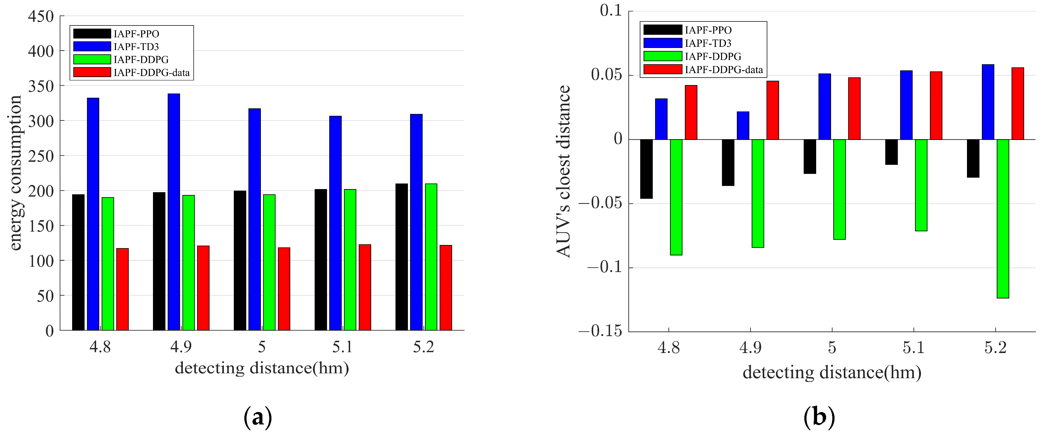
This paper also explores the effects of different remote sensing devices on AUV motion planning. The detection distance of the remote sensing equipment used in this paper during the simulation is 5 hm. Simulation of the motion planning at different detection distances is carried out to ensure that all four algorithms can accomplish the cruising task for multiple target points. The experimental results are presented in Figure 14. By comparing the energy consumption generated and the closest distance to the obstacle by the four algorithms, it becomes evident that the proposed algorithm completes the cruising task of multiple target points with the lowest energy consumption and safer navigation.
For estimating the computational resources consumed by the algorithm during its operation, it is essential to analyze the computational complexity. The computational complexity primarily considers the path generation based on the trained model, which involves executing a motion cruising task. Since only one iteration is performed, the dense neural network in the DRL algorithm determines the computational complexity. In the DNN, the computational complexity is O ( μ γ 2 ) . In the neural network, γ represents the number of layers, and μ represents the biggest number of layer neurons. In the neural network, the dimensionality in the input layer determines the number of neurons per layer, and the operational complexity is independent of the number of layers, so the computational complexity is O ( n 2 ) .

6. Conclusions and Future Work

In this paper, we introduced the TSP-IAPF-DDPG-data algorithm, which is a method to autonomously generate cruise sequences for multiple target points and generate the safest motion-planning path while consuming the least energy by using multi-source data for AUVs. The method improves the local optimum in APF and embeds the AUV’s motion model into the IAPF, which is combined with the TSP to automatically generate a cruising sequence to multiple target points in the 3D environment. The multi-source data and energy consumption models are embedded in the DDPG algorithm and combined with the IAPF algorithm, which contains a motion model, to optimize the path for cruising at multiple target points. We have simulated and compared the proposed algorithm with three related algorithms in multiple environments to demonstrate the superiority of the proposed algorithm in this paper. It also further verifies the proposed algorithm’s excellent performance when tracking trajectory with remote sensing information. The simulation data prove that the cruising path generated by this method has significant advantages in terms of minimum energy consumption, safe navigation, and turning smoothness.
In the future, we will work on multiple AUVs cruising and returning with minimal energy to multiple target points with path coverage. We will also work on migrating the algorithm to physical tests and further optimizing the proposed algorithm by using the data from physical tests.

Author Contributions

Conceptualization, T.X., X.W. and K.D.; methodology, T.X. and K.D.; software, T.X.; validation, T.X.; formal analysis, T.X., X.W. and K.D.; investigation, T.X.; resources, T.X., X.W. and Q.Z.; writing—original draft preparation, T.X.; writing—review and editing, T.X., Q.Z., K.D., X.W. and K.N.; visualization, T.X. and K.D.; supervision, Q.Z., X.W. and K.N.; project administration, Q.Z. and K.N.; funding acquisition, Q.Z. and K.N. All authors have read and agreed to the published version of the manuscript.

Funding

Shenzhen Science and Technology Innovation Committee (JCYJ20200109143006048, JCYJ20210324115813037).

Data Availability Statement

Not applicable.

Conflicts of Interest

The authors declare no conflict of interest.

References

  1. Sahoo, A.; Dwivedy, S.K.; Robi, P. Advancements in the field of autonomous underwater vehicle. Ocean Eng. 2019, 181, 145–160. [Google Scholar] [CrossRef]
  2. Stankiewicz, P.; Tan, Y.T.; Kobilarov, M. Adaptive sampling with an autonomous underwater vehicle in static marine environments. J. Field Robot. 2021, 38, 572–597. [Google Scholar] [CrossRef]
  3. Du, J.; Song, J.; Ren, Y.; Wang, J. Convergence of broadband and broadcast/multicast in maritime information networks. Tsinghua Sci. Technol. 2021, 26, 592–607. [Google Scholar] [CrossRef]
  4. Cao, X.; Ren, L.; Sun, C. Research on obstacle detection and avoidance of autonomous underwater vehicle based on forward-looking sonar. IEEE Trans. Neural Netw. Learn. Syst. 2022. [Google Scholar] [CrossRef]
  5. Wang, Z.; Zhang, Z.; Wang, J.; Jiang, C.; Wei, W.; Ren, Y. AUV-Assisted Node Repair for IoUT Relying on Multi-Agent Reinforcement Learning. IEEE Internet Things J. 2023. [Google Scholar] [CrossRef]
  6. Sun, B.; Zhang, W.; Li, S.; Zhu, X. Energy optimised D* AUV path planning with obstacle avoidance and ocean current environment. J. Navig. 2022, 75, 685–703. [Google Scholar] [CrossRef]
  7. Cao, X.; Chen, L.; Guo, L.; Han, W. AUV Global Security Path Planning Based on a Potential Field Bio-Inspired Neural Network in Underwater Environment. Intell. Autom. Soft Comput. 2021, 27, 391–407. [Google Scholar] [CrossRef]
  8. Zhu, D.; Cao, X.; Sun, B.; Luo, C. Biologically inspired self-organizing map applied to task assignment and path planning of an AUV system. IEEE Trans. Cogn. Dev. Syst. 2017, 10, 304–313. [Google Scholar] [CrossRef]
  9. Hao, K.; Zhao, J.; Li, Z.; Liu, Y.; Zhao, L. Dynamic path planning of a three-dimensional underwater AUV based on an adaptive genetic algorithm. Ocean Eng. 2022, 263, 112421. [Google Scholar] [CrossRef]
  10. Lin, C.; Han, G.; Du, J.; Bi, Y.; Shu, L.; Fan, K. A path planning scheme for AUV flock-based Internet-of-Underwater-Things systems to enable transparent and smart ocean. IEEE Internet Things J. 2020, 7, 9760–9772. [Google Scholar] [CrossRef]
  11. Yu, X.; Chen, W.-N.; Hu, X.-M.; Gu, T.; Yuan, H.; Zhou, Y.; Zhang, J. Path planning in multiple-AUV systems for difficult target traveling missions: A hybrid metaheuristic approach. IEEE Trans. Cogn. Dev. Syst. 2019, 12, 561–574. [Google Scholar] [CrossRef]
  12. Ma, X.; Yanli, C.; Bai, G.; Liu, J. Multi-AUV collaborative operation based on time-varying navigation map and dynamic grid model. IEEE Access 2020, 8, 159424–159439. [Google Scholar] [CrossRef]
  13. Wei, W.; Wang, J.; Fang, Z.; Chen, J.; Ren, Y.; Dong, Y. 3U: Joint design of UAV-USV-UUV networks for cooperative target hunting. IEEE Trans. Veh. Technol. 2022, 72, 4085–4090. [Google Scholar] [CrossRef]
  14. Zhang, C.; Cheng, P.; Du, B.; Dong, B.; Zhang, W. AUV path tracking with real-time obstacle avoidance via reinforcement learning under adaptive constraints. Ocean Eng. 2022, 256, 111453. [Google Scholar] [CrossRef]
  15. Bu, F.; Luo, H.; Ma, S.; Li, X.; Ruby, R.; Han, G. AUV-Aided Optical—Acoustic Hybrid Data Collection Based on Deep Reinforcement Learning. Sensors 2023, 23, 578. [Google Scholar] [CrossRef]
  16. Yang, P.; Cao, X.; Xi, X.; Du, W.; Xiao, Z.; Wu, D. Three-dimensional continuous movement control of drone cells for energy-efficient communication coverage. IEEE Trans. Veh. Technol. 2019, 68, 6535–6546. [Google Scholar] [CrossRef]
  17. Zhang, W.; Wang, N.; Wu, W. A hybrid path planning algorithm considering AUV dynamic constraints based on improved A* algorithm and APF algorithm. Ocean Eng. 2023, 285, 115333. [Google Scholar] [CrossRef]
  18. Zhang, J.; Liu, M.; Zhang, S.; Zheng, R.; Dong, S. Multi-AUV adaptive path planning and cooperative sampling for ocean scalar field estimation. IEEE Trans. Instrum. Meas. 2022, 71, 9505514. [Google Scholar] [CrossRef]
  19. Guo, J.; Hou, Y.; Liang, X.; Yang, H.; Xiong, Y. Mission-driven path planning and design of submersible unmanned ship with multiple navigation states. Ocean Eng. 2022, 263, 112363. [Google Scholar] [CrossRef]
  20. Wen, J.; Yang, J.; Wang, T. Path planning for autonomous underwater vehicles under the influence of ocean currents based on a fusion heuristic algorithm. IEEE Trans. Veh. Technol. 2021, 70, 8529–8544. [Google Scholar] [CrossRef]
  21. Yang, H.; Teng, X. Mobile robot path planning based on enhanced dynamic window approach and improved a algorithm. J. Robot. 2022, 2022, 2183229. [Google Scholar] [CrossRef]
  22. Yu, X.; Chen, W.-N.; Gu, T.; Yuan, H.; Zhang, H.; Zhang, J. ACO-A*: Ant colony optimization plus A* for 3-D traveling in environments with dense obstacles. IEEE Trans. Evol. Comput. 2018, 23, 617–631. [Google Scholar] [CrossRef]
  23. Sun, B.; Zhu, D.; Tian, C.; Luo, C. Complete coverage autonomous underwater vehicles path planning based on glasius bio-inspired neural network algorithm for discrete and centralized programming. IEEE Trans. Cogn. Dev. Syst. 2018, 11, 73–84. [Google Scholar] [CrossRef]
  24. Xing, T.; Wang, X.; Ding, K.; Ni, K.; Zhou, Q. Improved Artificial Potential Field Algorithm Assisted by Multisource Data for AUV Path Planning. Sensors 2023, 23, 6680. [Google Scholar] [CrossRef]
  25. Cao, X.; Sun, C.; Yan, M. Target search control of AUV in underwater environment with deep reinforcement learning. IEEE Access 2019, 7, 96549–96559. [Google Scholar] [CrossRef]
  26. Jiang, D.; Huang, J.; Fang, Z.; Cheng, C.; Sha, Q.; He, B.; Li, G. Generative adversarial interactive imitation learning for path following of autonomous underwater vehicle. Ocean Eng. 2022, 260, 111971. [Google Scholar] [CrossRef]
  27. Zhu, G.; Shen, Z.; Liu, L.; Zhao, S.; Ji, F.; Ju, Z.; Sun, J. AUV Dynamic Obstacle Avoidance Method Based on Improved PPO Algorithm. IEEE Access 2022, 10, 121340–121351. [Google Scholar] [CrossRef]
  28. Chu, Z.; Wang, F.; Lei, T.; Luo, C. Path planning based on deep reinforcement learning for autonomous underwater vehicles under ocean current disturbance. IEEE Trans. Intell. Veh. 2022, 8, 108–120. [Google Scholar] [CrossRef]
  29. Hadi, B.; Khosravi, A.; Sarhadi, P. Deep reinforcement learning for adaptive path planning and control of an autonomous underwater vehicle. Appl. Ocean Res. 2022, 129, 103326. [Google Scholar] [CrossRef]
  30. Su, N.; Wang, J.-B.; Zeng, C.; Zhang, H.; Lin, M.; Li, G.Y. Unmanned-Surface-Vehicle-Aided Maritime Data Collection Using Deep Reinforcement Learning. IEEE Internet Things J. 2022, 9, 19773–19786. [Google Scholar] [CrossRef]
  31. Fossen, T.I. Handbook of Marine Craft Hydrodynamics and Motion Control; John Wiley & Sons: Hoboken, NJ, USA, 2011. [Google Scholar]
  32. Phillips, A.; Haroutunian, M.; Murphy, A.J.; Boyd, S.; Blake, J.; Griffiths, G. Understanding the power requirements of autonomous underwater systems, Part I: An analytical model for optimum swimming speeds and cost of transport. Ocean Eng. 2017, 133, 271–279. [Google Scholar] [CrossRef]
  33. Khatib, O. Real-time obstacle avoidance for manipulators and mobile robots. Int. J. Robot. Res. 1986, 5, 90–98. [Google Scholar] [CrossRef]
  34. Lanfeng, Z.; Mingyue, K. 3D obstacle-avoidance for a unmanned aerial vehicle based on the improved artificial potential field method. J. East China Norm. Univ. 2022, 2022, 54. [Google Scholar]
  35. Ding, K.; Wang, X.; Hu, K.; Wang, L.; Wu, G.; Ni, K.; Zhou, Q. Three-dimensional morphology measurement of underwater objects based on the photoacoustic effect. Opt. Lett. 2022, 47, 641–644. [Google Scholar] [CrossRef] [PubMed]
  36. Butler, B.; Verrall, R. Precision Hybrid Inertial/Acoustic Navigation System for a Long-Range Autonomous Underwater Vehicle. Navigation 2001, 48, 1–12. [Google Scholar] [CrossRef]
  37. Zeng, Z.; Lian, L.; Sammut, K.; He, F.; Tang, Y.; Lammas, A. A survey on path planning for persistent autonomy of autonomous underwater vehicles. Ocean Eng. 2015, 110, 303–313. [Google Scholar] [CrossRef]
  38. Suh, Y.S. Attitude estimation by multiple-mode Kalman filters. IEEE Trans. Ind. Electron. 2006, 53, 1386–1389. [Google Scholar] [CrossRef]
  39. Campestrini, C.; Heil, T.; Kosch, S.; Jossen, A. A comparative study and review of different Kalman filters by applying an enhanced validation method. J. Energy Storage 2016, 8, 142–159. [Google Scholar] [CrossRef]
  40. Arulkumaran, K.; Deisenroth, M.P.; Brundage, M.; Bharath, A.A. Deep reinforcement learning: A brief survey. IEEE Signal Process. Mag. 2017, 34, 26–38. [Google Scholar] [CrossRef]
  41. Zeng, F.; Wang, C.; Ge, S.S. A survey on visual navigation for artificial agents with deep reinforcement learning. IEEE Access 2020, 8, 135426–135442. [Google Scholar] [CrossRef]
  42. Wang, X.; Gu, Y.; Cheng, Y.; Liu, A.; Chen, C.P. Approximate policy-based accelerated deep reinforcement learning. IEEE Trans. Neural Netw. Learn. Syst. 2019, 31, 1820–1830. [Google Scholar] [CrossRef] [PubMed]
  43. Hu, Z.; Wan, K.; Gao, X.; Zhai, Y.; Wang, Q. Deep reinforcement learning approach with multiple experience pools for UAV’s autonomous motion planning in complex unknown environments. Sensors 2020, 20, 1890. [Google Scholar] [CrossRef] [PubMed]
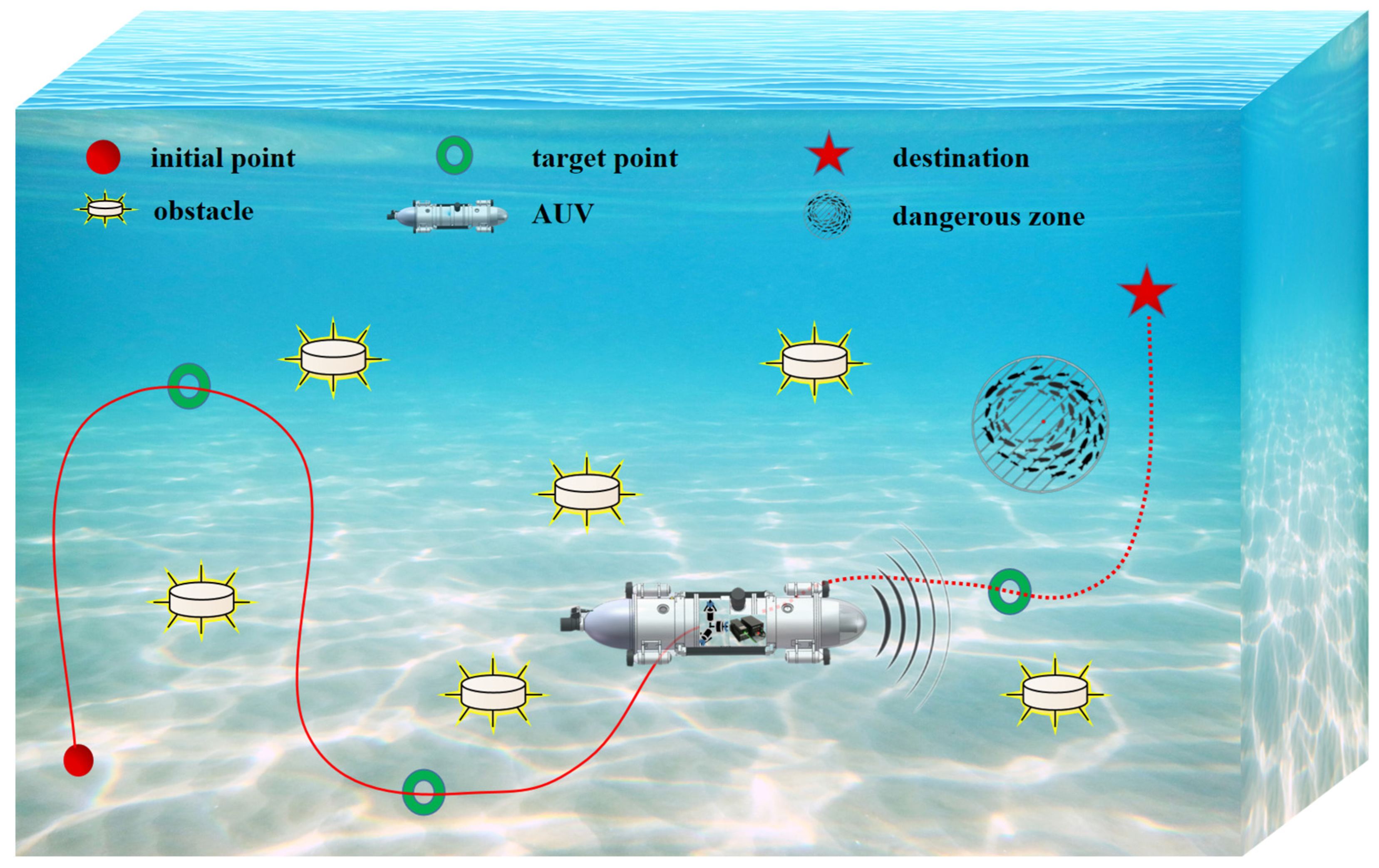
Figure 1. Schematic of multi-source-data-assisted AUV for multiple target point cruising.
Remotesensing 15 05607 g001
Figure 2. Kinematic and dynamic models for the AUV.
Remotesensing 15 05607 g002
Figure 3. The improvement strategies for the local optimum problem. (a) The improvement strategy for a single obstacle in the 2D environment. (b) The improvement strategy for multiple obstacles in the 2D environment. (c) The improvement strategy for a single obstacle in the 3D environment. (d) The improvement strategy for multiple obstacles in the 3D environment.
Remotesensing 15 05607 g003
Figure 4. Kalman filter process.
Remotesensing 15 05607 g004
Figure 5. Multi-source-data-assisted AUV motion planning based on the DDPG algorithm.
Remotesensing 15 05607 g005
Figure 6. Cruise sequence generated by TSP-IAPF.
Remotesensing 15 05607 g006
Figure 7. Reward curves generated by four DRL algorithms.
Remotesensing 15 05607 g007
Figure 8. The planned 3D paths from the four algorithms: (a) top view; (b) 3D view.
Remotesensing 15 05607 g008
Figure 9. The four algorithms’ generated motion data. (a) Steering angle. (b) Attack angle. (c) Pitch angle. (d) Nearest distance to the obstacle. (e) Velocity. (f) Acceleration.
Remotesensing 15 05607 g009
Figure 10. Energy consumption, the closest distance to the obstacle, path length, and navigation time for the four algorithms under Monte Carlo simulation. (a) Simulation of energy consumption and closest distance to the obstacle. (b) Simulation of path length and navigation time.
Remotesensing 15 05607 g010
Figure 11. (a,b) Motion-planning paths are generated by four algorithms in a dynamic environment.
Remotesensing 15 05607 g011
Figure 12. Trajectory-tracking curve for AUV under remote sensing error. (a) Top view of trajectory tracking curve. (b) Three-dimensional view of trajectory-tracking curve.
Remotesensing 15 05607 g012
Figure 13. Energy consumption and closest distance to the obstacle for different remote sensing detection distances: (a) energy consumption; (b) nearest distance to the obstacle.
Remotesensing 15 05607 g013
Figure 14. Trajectory-tracking error for AUV.
Remotesensing 15 05607 g014
Table 1. Capacity parameters and hyperparameters during the training process.
CategoryParameter NameParameter Values
Mechanical parametersVelocity1~10 m/s (0.01~0.10 hm/s)
Steering angle−40°/s~40°/s
Attack angle−40°/s~40°/s
Pitch angle−50°~50°
HyperparameterExperience replay buffer2 × 106
Batch size128
Max episode1000
Max step500
Actor learning rate0.001
Critic learning rate0.001
Soft update rate0.01
Additional information. In the steering angle, the positive value represents the left turn, and the negative value represents the right turn. In the attack angle, the positive value represents the climbing angle, and the negative value represents the descent angle. In the pitch angle, the positive value represents the elevation angle, and the negative value represents the depression angle.
Table 2. Experimental data 1.
NameIAPF-PPOIAPF-TD3IAPF-DDPGIAPF-DDPG-Data
es188.242749317.011388194.030737118.264115
cd−0.0272840.051236−0.0779430.048216
as1.90356313.9842654.0031032.922921
aa1.87628511.7849651.2431110.945653
Me50.00001850.00001850.00001850.000018
Mv10.00000010.00000010.00000010.000000
Ma4.4999849.0000009.0000004.999958
pl25.69247731.36952826.29385127.032355
rt545957553567
The meaning of the abbreviations: es denotes the energy consumption. cd denotes the closest distance, and negative values represent the distance from the entry obstacle. The rest of the data are expressed in absolute values. as denotes the arithmetic mean of the steering angle. aa denotes the arithmetic mean of the attack angle. Me denotes the maximum climb angle. Mv denotes the maximum velocity. Ma denotes the maximum acceleration. pl denotes the path length. rt denotes the navigation time.
Table 3. Experimental data 2.
NameIAPF-PPOIAPF-TD3IAPF-DDPGIAPF-DDPG-Data
es162.028648991.704624282.105936176.921956
cd−0.041092−0.095522−0.0244990.007177
as3.3652457.6676073.3858322.942140
aa1.3130242.5526701.6492191.101778
Me50.00001850.00001850.00001850.000018
Mv9.97918510.00000010.00000010.000000
Ma5.6375159.0000009.0000009.000000
pl28.72347836.95316226.60011427.097279
rt1052125211601012
Disclaimer/Publisher’s Note: The statements, opinions and data contained in all publications are solely those of the individual author(s) and contributor(s) and not of MDPI and/or the editor(s). MDPI and/or the editor(s) disclaim responsibility for any injury to people or property resulting from any ideas, methods, instructions or products referred to in the content.