1. Introduction
The Advanced Clear-Sky Processor for Ocean (ACSPO; see the abbreviations at the end of this paper) sea surface temperature (SST) enterprise system, designed and maintained at NOAA, provides SSTs from multiple satellites in geostationary (GEO) and low Earth orbits (LEO). Full-mission reprocessed high-resolution (~1 km or higher at nadir) ACSPO SST data from VIIRS (flown onboard afternoon orbit ‘PM’ satellites NPP, N20 and N21) and AVHRR FRAC (flown onboard mid-morning orbit ‘AM’ satellites Metop-A, B and C) are publicly available [
1,
2]. The ACSPO VIIRS SST dataset extends back to February 2012 (earliest NPP SST data), and AVHRR FRAC SST is available back to December 2006 (earliest Metop-A SST data).
This work documents the first ACSPO SST Reanalysis (RAN1) dataset produced from two Moderate Resolution Imaging Spectroradiometers (MODIS). The first MODIS was launched on 18 December 1999 onboard the Terra satellite, and the second was launched on 4 May 2002 onboard the Aqua satellite. The MODIS RAN1 SSTs go back to the earliest available high-quality MODIS Brightness Temperatures (BTs) in the thermal emissive bands (TEBs) (24 February 2000 for Terra and 4 July 2002 for Aqua). Data from Collection 6.1 L1b are used [
3,
4]. As of the time of writing, both MODIS sensors remain active, with the RAN1 data updated monthly in a delayed mode with an approximately two-month latency [
5]. The over two-decade, continuous, long-term time series of high-resolution SST data make the MODIS record unique. No other currently available high-resolution satellite SST dataset matches the longevity, consistency, and quality of Aqua and Terra. Similar to its predecessor, AVHRR, and successor, VIIRS, MODIS is an Earth-viewing, cross-track-scanning instrument. Of its 36 spectral bands, covering from 0.4 to 14.4 µm, three mid-wave infrared bands (MWIR; bands 20, 22, and 23) and three long-wave infrared bands (LWIR; bands 29, 31 and 32), all with a 1 km resolution at nadir, are positioned in three atmospheric windows and are suitable for SST retrieval.
The MODIS RAN1 dataset is produced in L2P (original swath projection), L3U (0.02° gridded uncollated), and L3C (0.02° gridded collated) formats. All products are compliant with the Group for High-Resolution SST (GHRSST) Data Specification v2 (GDS2) standard [
6]. As of the time of writing, a full archive of Aqua and Terra L3C data is available at NOAA CoastWatch [
5]. Archival of the full L2P, L3U, and L3C records at JPL PO.DAAC is being explored. The L2P data are reported in 10 min granules (144 files/24 h) with a ~950 GB/year/satellite data volume. The 0.02° L3U data are produced from L2P files and reported in same-size 10 min granules (144 files/24 h), with a ~130 GB/year/satellite data volume. The 0.02° L3C data are produced by collating L3U SST data from multiple satellite overpasses and reported in two files/24 h, one for day and one for night, with ~125 GB/year/satellite data volume. Only data of the highest quality level, QL = 5 (classified as ‘clear-sky’ by the ACSPO Clear-Sky Mask, ACSM [
7]) are recommended for use. All evaluations of the MODIS RAN1 dataset in this study are based on L2P data. The performance of the L3U and L3C SST products (in terms of global mean bias and standard deviation against in situ SSTs, and coverage) is comparable or superior to that of L2P, and therefore, their evaluation is omitted here in the interest of space.
Note that ACSPO MODIS RAN1 is not the first or only full-mission reprocessed MODIS SST dataset. The other dataset available at the time of writing is the NASA R2019 SST, which is also based on MODIS Collection 6.1 L1b data. The previous version, R2014, was documented in [
8], with R2019 updates summarized in [
9]. The NASA R2019 SST dataset is available in L2P format and in various flavors of L3 (including daily, weekly, monthly and annual averages) at spatial resolutions of 4.63 km and 9.26 km [
10,
11]. The NASA R2019 L2P dataset will be discussed later in this work, to place the performance of the ACSPO RAN1 SST in context. Standard metrics, such as the accuracy (global mean bias with respect to quality-controlled in situ data from drifters and tropical moorings, DTMs), precision (corresponding standard deviation), and the relative size of their clear-sky domains are evaluated. Sensitivity to true SST is another important metric of SST performance [
12,
13]. RAN1 sensitivities are discussed later in this work. The sensitivity of the NASA SST is unknown to us, and this metric cannot be compared with the ACSPO. Comparisons with ACSPO VIIRS SSTs [
1] will also be performed where appropriate. The primary motivation for producing the MODIS RAN1 dataset with the NOAA ACSPO system was to facilitate its inclusion in the NOAA multi-sensor L3S-LEO high-resolution SST product, which currently only includes data from JPSS VIIRSs and Metop-FG AVHRR FRACs [
1,
2,
14]. NOAA users have expressed interest in including MODIS in the L3S-LEO and extending its time series back to 2000.
This work is organized as follows:
Section 2 discusses the Terra and Aqua orbits.
Section 3 provides an overview of the ACSPO MODIS algorithms with emphasis on SST retrievals and a comparison with the ACSPO VIIRS and AVHRR algorithms.
Section 4 validates MODIS SSTs against iQuam in situ SSTs from drifting and tropical moored buoys (DTMs) with complementary validation against Argo floats (AFs) presented in
Appendix A [
15].
Section 5 documents the mitigation/debiasing of residual calibration artifacts in the MODIS TEBs, including discontinuities and drifts of BTs in individual bands. The debiasing is performed using comparisons of observed MODIS BTs with modeled BTs, obtained using the NOAA Community Radiative Transfer Model (CRTM) [
16,
17,
18].
Section 6 summarizes the results of this study and discusses future work.
3. ACSPO Algorithms
In ACSPO, the SST is retrieved from clear-sky BTs in MODIS bands 20, 31, and 32, centered at 3.7, 11, and 12 µm, respectively. During the daytime (pixels with solar zenith angle ≤ 90°), two reflective solar bands (1 and 2) centered at 0.65 and 0.86 µm are additionally used by the ACSM [
7].
The ACSPO files report the ‘subskin’ SST (often considered a proxy for temperature at a ~1 mm depth) in the ‘sea_surface_temperature’ variable. Note that satellite infrared radiometers are sensitive to skin SST (effective temperature of the top ~10 µm layer), which is typically several tenths of a kelvin colder than the subskin SST due to radiative losses at the ocean surface [
6]. Since skin SSTs available from shipborne infrared radiometers are very scarce and insufficient for the calibration and validation of satellite SSTs, satellite retrievals are often trained against much more numerous conventional in situ SSTs measured by drifting and tropical moored buoys (DTMs), typically using sampling temperatures at ~20 cm to ~1 m depths. Some data producers (e.g., [
8,
9]) subtract 0.17 K (the mean cold skin effect) from the derived SSTs and call their products ‘skin’ SST. (Note that this offset should be added back when ‘skin’ SSTs are validated against the same DTM data to ensure an expected zero bias). Other SST groups, including OSISAF [
22] and ACSPO, do not subtract the 0.17 K and call their products ‘subskin’ (saving the need to add this offset back at the validation stage). The ‘skin’ and ‘subskin’ terms are thus merely two different conventions that are currently in use. To emphasize this fact, they are bracketed with quote/unquote symbols in the remainder of the paper.
In compliance with the GDS2 standard [
6], ACSPO files also report two sensor specific error statistics (SSES) variables for each pixel, bias and standard deviation, which are estimated vs. DTM SSTs. Subtracting the SSES bias (stored in the ‘sses_bias’ variable) from the ‘subskin’ SST gives the ACSPO ‘depth’ SST (another convention, adopted in the ACSPO products), a better proxy for the SST at depths of ~0.2–1.0 m typically sampled by DTMs. Both the ACSPO ‘subskin’ and ‘depth’ SSTs are calculated using the nonlinear SST (NLSST) equation [
12,
23]. The main difference between the two is that the ‘subskin’ SST is calculated using a global regression algorithm (with only two sets of regression coefficients, one set for night and another set for day). In contrast, the ‘depth’ SST is calculated using a piecewise regression algorithm, where the retrieval domain is stratified into multiple segments, each with its own regression coefficients [
24]. Owing to segmentation of the retrieval domain and the larger number of trainable parameters, the piecewise regression SST agrees more closely with the DTM SSTs (cf.
Section 4). However, as discussed later in this section, its retrieval sensitivity is considerably lower than that for global regression due to the significant contribution from prior information, such as the first-guess SST, resulting in reduced spatial and temporal SST gradients [
12,
13].
At night (pixels with solar zenith angle > 90°), the SST is retrieved using a three-band equation of the following form:
Here,
T3.7,
T11, and
T12 are MODIS BTs in bands centered at 3.7, 11, and 12 µm,
, and
θ is the satellite view zenith angle (VZA). During the daytime, the same equation is used, except that the terms with the 3.7 µm BTs,
, are excluded due to contamination from reflected and scattered solar radiation:
For MODIS, the VZA range is ±65° with the convention that the VZA is positive at the beginning of the scan and negative at its end. The regression coefficients
ai and
bi have been trained using five years (2016–2021) of MODIS BTs matched with iQuam DTM SSTs. The regression coefficients are ‘static’ (i.e., calculated only once and used throughout the full Aqua and Terra missions). This is in contrast to ‘variable’ coefficients (e.g., those employed in ACSPO AVHRR FRAC RAN1 [
2]), which are recalculated daily.
Table 1 lists the contributions (loads) of each MODIS band to the ‘subskin’ SST calculated using Equations (1) and (2). The individual band loads are defined as global mean partial derivatives of NLSST Equations (1) and (2) with respect to the BTs in each band.
Table 1 shows that, for both night and day, the sum of the BT loads is close to one, as expected. At night, transparent band 20 centered at 3.7 µm is the main contributor to the MODIS SST with mean loads of +1.30/+1.35 for Terra/Aqua, respectively. The longwave split-window bands contribute much less, with weights of +0.34/+0.37 for
(suggesting that this band does help with atmospheric correction) and only −0.02/−0.06 for
(suggesting that this band contributes only minimally). During the daytime, the loads on the split-window bands are much larger, ~+4 for
and ~−3 for
, suggesting that, in the absence of the transparent 3.7 µm band, both LWIR bands are essential for atmospheric correction. A side effect of the large contribution of the BT difference term is the amplification of noise present in BTs, which propagates into the retrieved SST [
25]. In all ACSPO SST products from LEO satellites, noise in the BT difference terms is mitigated using a special smoothing algorithm, which extracts the ‘SST-correlated component’ from the BT differences and smooths only this ‘residual’ to prevent the smoothing of real SST features [
26].
The larger loads on the LWIR bands in the daytime retrievals make them more sensitive to band-specific calibration drifts. In
Section 5, we use the magnitudes and signs of individual BT loads to link the drift in retrieved SST to drifts in individual BTs.
An important metric for SST retrieval algorithms is the sensitivity of the retrieved SST to the true SST [
12,
13]. This is obtained by differentiating Equations (1) and (2) with respect to the SST, with the partial derivatives of BTs computed using CRTM [
16,
17,
18]). Ideally, the sensitivity should be close to 1, uniform in space, and stable over time. Lower sensitivity values indicate a reduced ability to resolve spatial gradients and temporal variations in the retrieved SST.
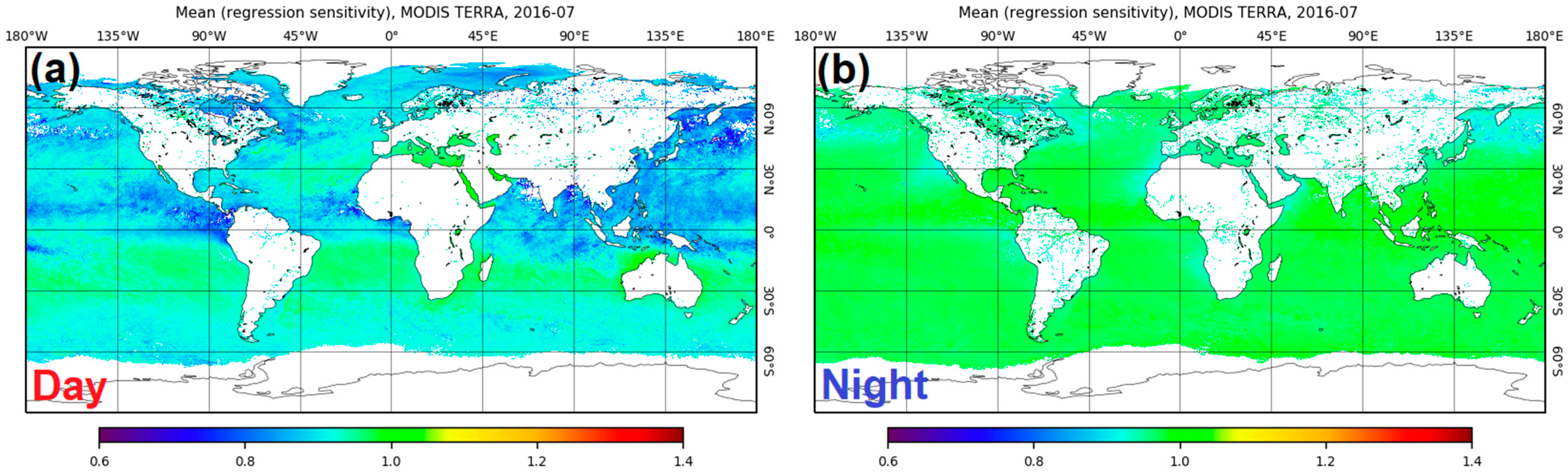
Table 1 lists the global mean ACSPO MODIS ‘subskin’ SST sensitivities to the true SST and the corresponding global standard deviations. The mean sensitivities are very consistent between Aqua and Terra, with a higher sensitivity at night (0.970 ± 0.003) and lower during the day (0.924 ± 0.002). The corresponding standard deviations are 0.015 ± 0.001 at night and 0.053 ± 0.001 during the daytime.
Figure 2 shows the global distribution of the day- and nighttime sensitivities. The daytime sensitivity shows more spatial variability with lower values found in humid regions. The nighttime sensitivity is closer to 1 and is more spatially uniform due to the use of the atmospherically transparent MWIR band 20. Both MODIS sensitivities are slightly lower than for VIIRS (~0.99 for night and 0.96 for daytime [
1]). This is likely due to the use of the LWIR M14 band centered at 8.6 µm for VIIRS retrievals, whereas for MODIS, this band is unusable [
1,
27,
28].
Table 1 also lists the load on the first-guess SST (i.e., the partial derivative of Equations (1) and (2) with respect to
). The contribution of the first-guess SST is minimal at night (<0.01) and moderate during the daytime (0.11–0.12). Recall that the linear Multi-Channel SST (MCSST) is often used at night due to the availability of the very transparent 3.7 µm band [
13]. During the daytime, the NLSST formulation is essential and a higher sensitivity to the first-guess SST is expected.
Equations (1) and (2) are the same as those used for ACSPO AVHRR FRAC SST retrievals [
2], except for the last term that is proportional to the VZA (θ), which is not present in the ACSPO FRAC or VIIRS SST algorithms [
1,
2]. This is the only term in Equations (1) and (2) that is not symmetrical with respect to nadir. The reason for its inclusion in MODIS SST retrievals is historical. Early in the Terra MODIS mission, significant response versus scan angle (RVS) biases caused by the angular dependence of the MODIS scan mirror reflectivity were discovered in the LWIR bands [
29]. The RVS issue resulted in large (~2 K) SST biases across the Terra MODIS scan [
8]. The RVS issue was addressed in MODIS Collection 3, with further refinements in later collections. MODIS RAN1 uses Collection 6.1 L1b data [
3,
4]. We found that the contribution of the VZA term to the SST is small for both Terra and Aqua (<0.01 K at night and <0.10 K during the daytime).
Equations (1) and (2) also differ from the VIIRS SST algorithm in that MODIS band 29 (centered at 8.6 µm) is not used due to its degraded performance (electronic crosstalk in both Aqua and Terra MODISs [
1,
27,
28]). The absence of the 8.6 µm band results in a slightly degraded quality for the MODIS SST compared to the VIIRS in terms of the precision (standard deviation with respect to the in situ SST; see
Section 4) and a lower sensitivity to the true SST. The degradation of both the precision and sensitivity is more pronounced during the daytime, when atmospherically transparent MWIR bands cannot be used for SST retrievals.
ACSPO v2.80 ‘depth’ SSTs are calculated using the same Equations (1) and (2), except a piecewise regression algorithm is employed where the retrieval domain is split into multiple segments, with each segment having its own set of regression coefficients,
ai and
bi [
24]. In ACSPO files, the ‘depth’ SST can be obtained by subtracting the ‘sses_bias’ from the ‘sea_surface_temperature’. As will be shown in
Section 4, the precision (global standard deviation with respect to in situ SST) is considerably improved for ‘depth’ compared to the ‘subskin’ SST. However, this comes at the price of a lower sensitivity. The global mean ACSPO MODIS night/day ‘depth’ SST sensitivity is only ~0.70/0.65, compared to ~0.97/0.92 for the ‘subskin’ SST. Validation of both the ACSPO ‘subskin’ and ‘depth’ SSTs against various in situ SSTs from the iQuam online system [
15] is presented in
Section 4.
The ACSPO and NASA MODIS systems both employ regression SST algorithms, stratified by day and night, but with several substantial differences [
8,
9,
10,
11]. First, ACSPO produces ‘subskin’ SSTs in which the regressions are trained against in situ data (separately for day and night) and then employed in retrievals as-is (i.e., with no changes to the derived coefficients). In contrast, NASA produces the ‘skin’ SST, which is trained against in situ data similarly to ACSPO, but the regression offset is then adjusted by −0.17 K, before making retrievals. The second difference is that ACSPO ‘subskin’ SSTs are derived using only one global set of regression coefficients for day, and one for night. In contrast, the NASA regression employed in R2019, is additionally stratified by month-of-the-year and seven latitudinal bands (below 40°S, four 20°-wide bands from 40°S to 40°N, one band between 40°N and 60°N, and one band for arctic regions above 60°N) [
8,
9]. The monthly segmentation is performed only once (with the exception of the early Terra period) and used for subsequent years. The specific forms of the regressions also differ. The daytime regressions are most similar, both employing split-window NLSSTs with two LWIR bands, 31 and 32, centered at 11 and 12 µm. At night, the ACSPO SST employs a three-band NLSST Equation (1) with one MWIR (20) and two LWIR bands (31 and 32) [
1,
2]. NASA, on the other hand, reports two products: SST (produced with the same daytime split-window LWIR NLSST, for consistency with the daytime retrievals), and a MODIS-unique SST4 (produced with the MWIR-only split-band algorithm, using bands 22 and 23 centered at 3.9 and 4.0 µm). Our additional analyses (not shown here) suggest, consistently with analyses performed by the R2019 producers, that the precision of the MWIR SST4 is considerably improved over that of the LWIR SST [
8].
Section 4 consistently compares NASA and ACSPO SST validation metrics, including the accuracy, precision, and clear-sky ratio (but excluding the sensitivity, which was not available to us from the R2019).
The ACSM is a crucial component of the ACSPO system [
7]. Its role is to identify clear-sky pixels in which accurate SST retrievals can be made. The ACSM is often colloquially referred to as the ‘cloud mask’, because the vast majority of the masked pixels occur due to obstruction by clouds. However, pixels can also be masked for other reasons, such as sensor issues, aerosol contamination, or atmospheric conditions that are not represented in the SST algorithm training set. The ACSM is documented in [
7] with recent additions described in [
1], such as reduced over-screening of dynamic SST regions and the removal of redundant filters based on the simulated BTs. In all ACSPO L2P files from LEO satellites, the SST is reported for all ocean/water pixels (all-sky domain), while 0.02° Level 3 files only contain clear-sky data to reduce the file size. To apply the ACSM, the user should only select pixels with QL = 5 (stored in the ‘quality_level’ variable). Additional information about land/ice coverage and day/night designation for each pixel is included in the ‘l2p_flags’ variable.
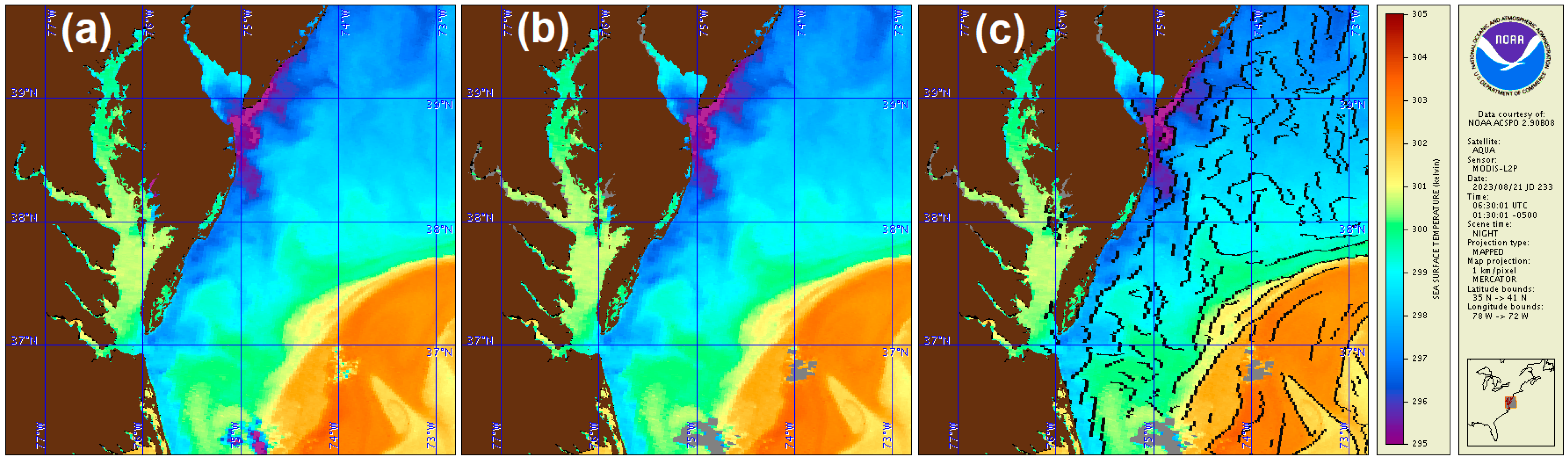
Figure 3 shows an example of Aqua MODIS nighttime ‘subskin’ SST imagery with and without the ACSM applied. Also shown is information about thermal fronts included in the ‘sst_front_position’ (binary indicator of the thermal SST front position) and ‘sst_gradient_magnitude’ (in units of K/km) variables.
MODIS is a multi-detector sensor with 10 detectors per band (compared to 16 for VIIRS and 24 for the planned METimage sensor). Individual calibration of each detector may result in imagery striping, if they are not accurately co-registered. Any striping artifacts in BTs are amplified by the BT difference terms in SST retrieval Equations (1) and (2), resulting in increased SST striping. In ACSPO SST products, VIIRS and MODIS BTs go through a de-striping preprocessing step [
31]. Another consequence of the multi-detector design is the well-known bow-tie effect, where imagery is distorted (more so away from nadir), and pixels near the scan edge overlap. There is also a discontinuity in the imagery between neighboring pixels from different scans. Distorted imagery degrades the ACSM, which uses spatial-window-based algorithms to identify clear-sky pixels. For this reason, in ACSPO v2.50 and later versions, imagery is resampled to correct for bow-tie distortion in all MODIS and VIIRS ACSPO data [
32]. The same approach will be taken for the future METimage sensor. Another motivation for bow-tie correction is the new ACSPO thermal fronts product, which requires spatially continuous SST imagery.
Although both the MODIS and VIIRS have similar multi-detector designs, the onboard processing of sensor data differs. In order to reduce the data volume and limit pixel size growth at high VZAs, VIIRS uses an aggregation scheme where three measurements are averaged near nadir (below 31.72°), two at intermediary scan angles (31.72–44.86°), and no aggregation is performed at high scan angles (above 44.86°) [
19]. No such aggregation is performed on MODIS, whose pixel grows from nadir to scan edge much greater (1–5 km in the across-track and 1–2 km in the along-track directions) than on VIIRS (0.75 to 1.6 km for both along and across track directions) [
19,
33]. Another difference in post-processing is ‘bow-tie removal’, where overlapping VIIRS pixels at scan angles above 31.72° are replaced with fill values to further reduce the data volume. In contrast, overlapping MODIS pixels are included in L1b data. Note that the detailed handling of bow-tie distortion and onboard deletion is only relevant for users of ACSPO L2P data and does not affect derived ACSPO L3 data, except indirectly via the improved ACSM, which may be propagated from L2P data.
4. Validation of the ACSPO MODIS RAN1 SST
This section presents the validation results for the Terra and Aqua ‘subskin’ and ‘depth’ L2P SSTs against quality-controlled in situ SSTs from the NOAA iQuam v2.10 online system [
15]. Note that this section analyzes the final ACSPO MODIS RAN1 dataset, produced from debiased BTs, where discontinuities and gradual drifts in the MODIS TEBs have been mitigated, as described in
Section 5 and
Appendix B. Note also that the performance of L3U and L3C data is comparable to that of L2P and is not analyzed here.
The included sources of in situ data are drifting and tropical moored buoys (DTMs), as well as Argo floats (AFs; presented in
Appendix A). Due to the sparse geographical coverage by drifting buoys near the equator, they are often grouped together with tropical moorings. Validation against the DTMs is presented in
Section 4.1. For an intercomparison of satellite and in situ SST data in SQUAM [
34], all satellite pixels within a space/time interval of [10 km × 30 min] of an in situ SST measurement are used. This results in ‘one-to-many’ matchup datasets (MDSs) where each in situ SST measurement is matched up with multiple satellite pixels. The exact number of satellite pixels matched up with a given in situ measurement depends on the size of the satellite pixel (for MODIS, 1–5 km depending on VZA) and the local clear-sky fraction near the in situ SST measurement. Only in situ SSTs with the highest iQuam quality level (QL = 5) are used.
The two main SST validation metrics are the accuracy (global mean bias with respect to DTMs) and precision (corresponding standard deviation). No formal set of NOAA SST requirements/specs exists for MODIS. In this work, we adopt the NOAA JPSS VIIRS requirements of ±0.2 K for accuracy and 0.6 K for precision [
35]. A recent addition to the JPSS SST specs is that accuracy and precision requirements must be met in a clear-sky domain covering at least 18% of the global ocean or more. This additional requirement is motivated by the fact that the specs are easier met with an overly conservative clear-sky mask in a reduced clear-sky domain.
Section 4.1 shows that specs are exceeded by a wide margin for both ‘subskin’ and ‘depth’ SSTs.
Appendix A shows that when compared to fully independent AFs, the requirements are also met, with the exception of the Aqua daytime ‘subskin’ SST. The reason is that the AF SSTs are measured deeper (~5 m) compared to DTMs (~0.2–1.0 m), causing larger and a more variable diurnal thermocline present at the 1:30 p.m. Aqua daytime overpass time.
Table 2 lists the Aqua and Terra mean clear-sky ratios (CSRs) for both daytime and nighttime SSTs for one full year (2019) of data. Note that the CSRs do not significantly vary from year-to-year, so one-year statistics are representative for whole missions.
NPP and N20 VIIRS CSRs are also included, to place the MODIS RAN1 data in perspective. The 18% CSR requirement is met for all satellites, with CSRs ranging from 18.8% (NPP night) to 20.6% (Terra night). Keep in mind that cloud coverage has a diurnal cycle, possibly leading to different CSRs from Aqua (1:30 a.m./p.m.) and Terra (10:30 a.m./p.m.), whereas the NPP and N20 have similar LEXTs to Aqua [
1]. Aqua CSRs are slightly higher than the NPP/N20 both at night (19.1 vs. 18.8%) and during the day (20.4 vs. 19.9%), likely due to a narrower MODIS VZA range and a larger fraction of near-nadir pixels. In addition, the Aqua retrieval sensitivity is somewhat lower compared to VIIRS, as discussed in
Section 3 (0.93 vs. 0.96 in the day and 0.97 vs. 0.99 during the night). A higher SST retrieval sensitivity typically results in a lower CSR, due to reliance of the current ACSM adopted in ACSPO v2.80, on the delta between the satellite and first-guess SST [
7].
Another important validation metric is the long-term stability of satellite SSTs characterized as the temporal drift in accuracy over a satellite’s mission (typically due to the TEB calibration drift). No formal NOAA requirements exist for stability, so we adopt the (A)ATSR Reprocessing for Climate (ARC) project target stability of 5 mK/year (0.05 K/decade) [
36].
Section 4.2 analyzes the time series of MODIS SSTs against DTMs and shows that both Terra and Aqua SSTs meet and exceed the target stability by a wide margin.
4.1. Validation of MODIS RAN1 SST against Drifting and Tropical Moored Buoys (DTMs)
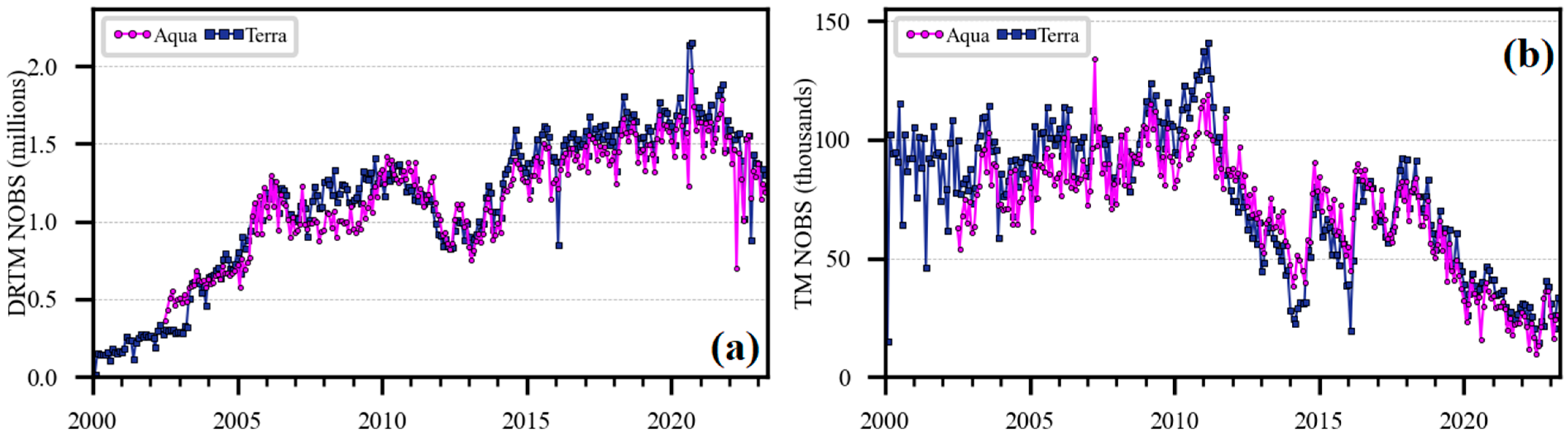
Figure 4a shows the time series of the monthly number of MODIS RAN1 matchups with DTMs. To demonstrate the relative contributions of drifters and tropical moorings (TMs) to the global validation statistics,
Figure 4b shows a similar plot but for the TMs only. More than 10
5 monthly DTM matchups are available for the entire MODIS mission, at all times, but the relative contribution to NOBS from TMs vs. drifters has varied considerably over time. In 2000, the majority of the matchups were from the TMs. For example, in June 2000, 0.91 × 10
5 out of 1.44 × 10
5 Terra matchups were from TMs, or about 63%. Since 2000, the number of drifters has increased considerably, and newer drifters report SST measurements more frequently (hourly or more often), resulting in an increased number of matchups. On the other hand, the number of TMs reporting SSTs has declined since 2011, with a 75% drop in TM matchups from 2000 to the present time. In recent years, validation statistics have been dominated by drifters. For example, in June 2022, only 2 × 10
4 out of 1.4 × 10
6 total DTM matchups come from TMs, only about 1.4%.
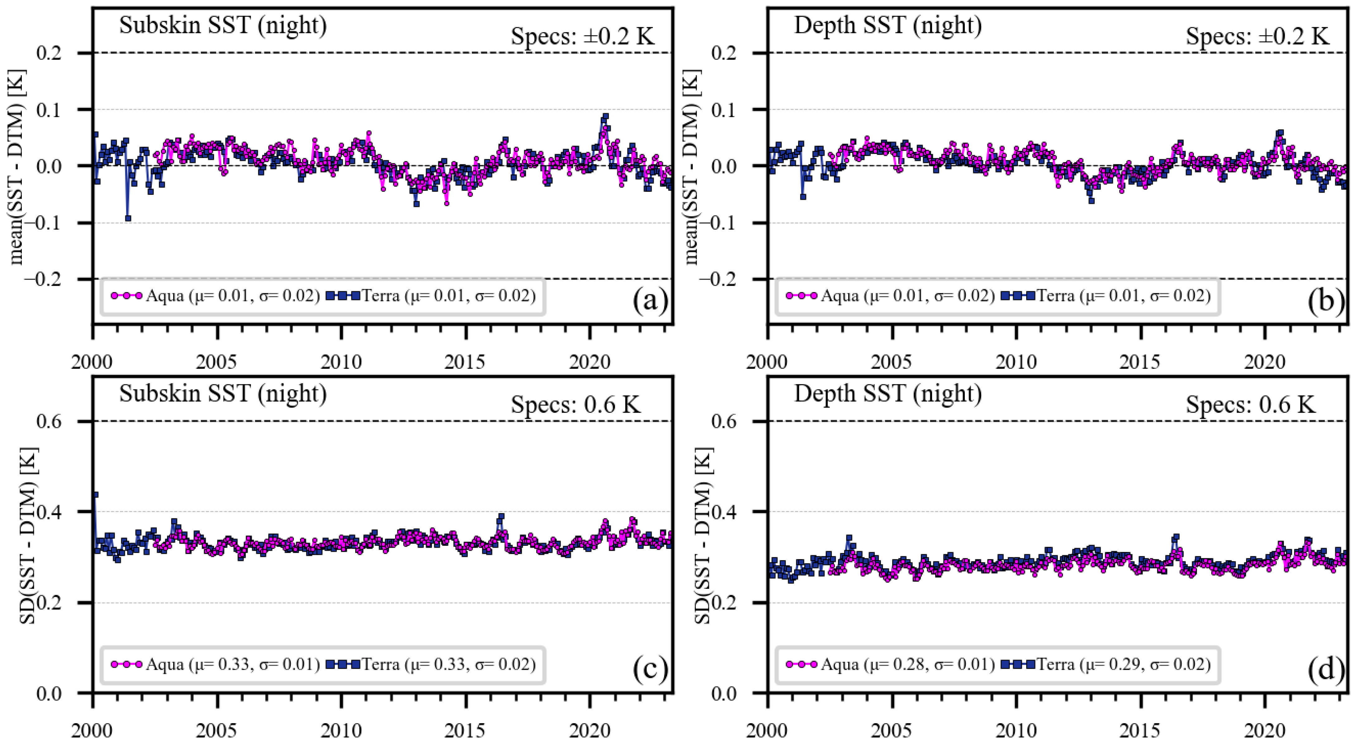
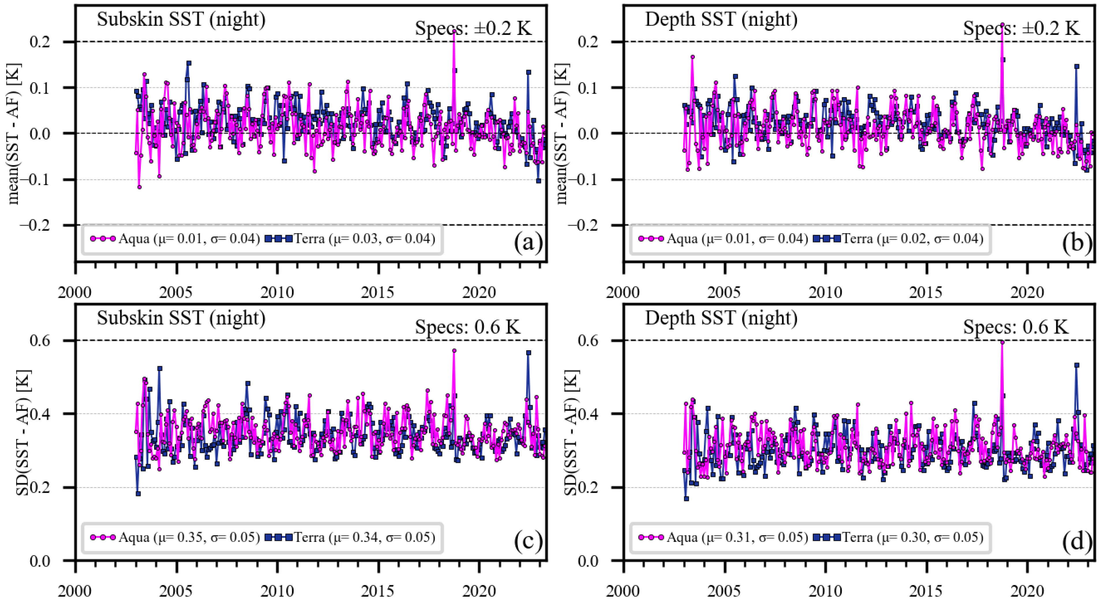
Figure 5 shows the monthly aggregated time series of the accuracy (global mean bias) and precision (corresponding standard deviation) of the MODIS nighttime ‘subskin’ and ‘depth’ SSTs against the DTMs. The NOAA specs for accuracy (±0.2 K) are met and exceeded for both Aqua and Terra. Typically, the accuracy is within a ±0.1 K corridor and is often within ±0.05 K. The precision requirement of 0.6 K is also met and exceeded, by a wide margin. As expected, the precision of the ‘depth’ SST (0.28–0.29 K) is improved compared to that of the ‘subskin’ SST (0.33 K). The Aqua and Terra accuracies and precisions agree very closely, with no visible systematic temporal change in the time series.
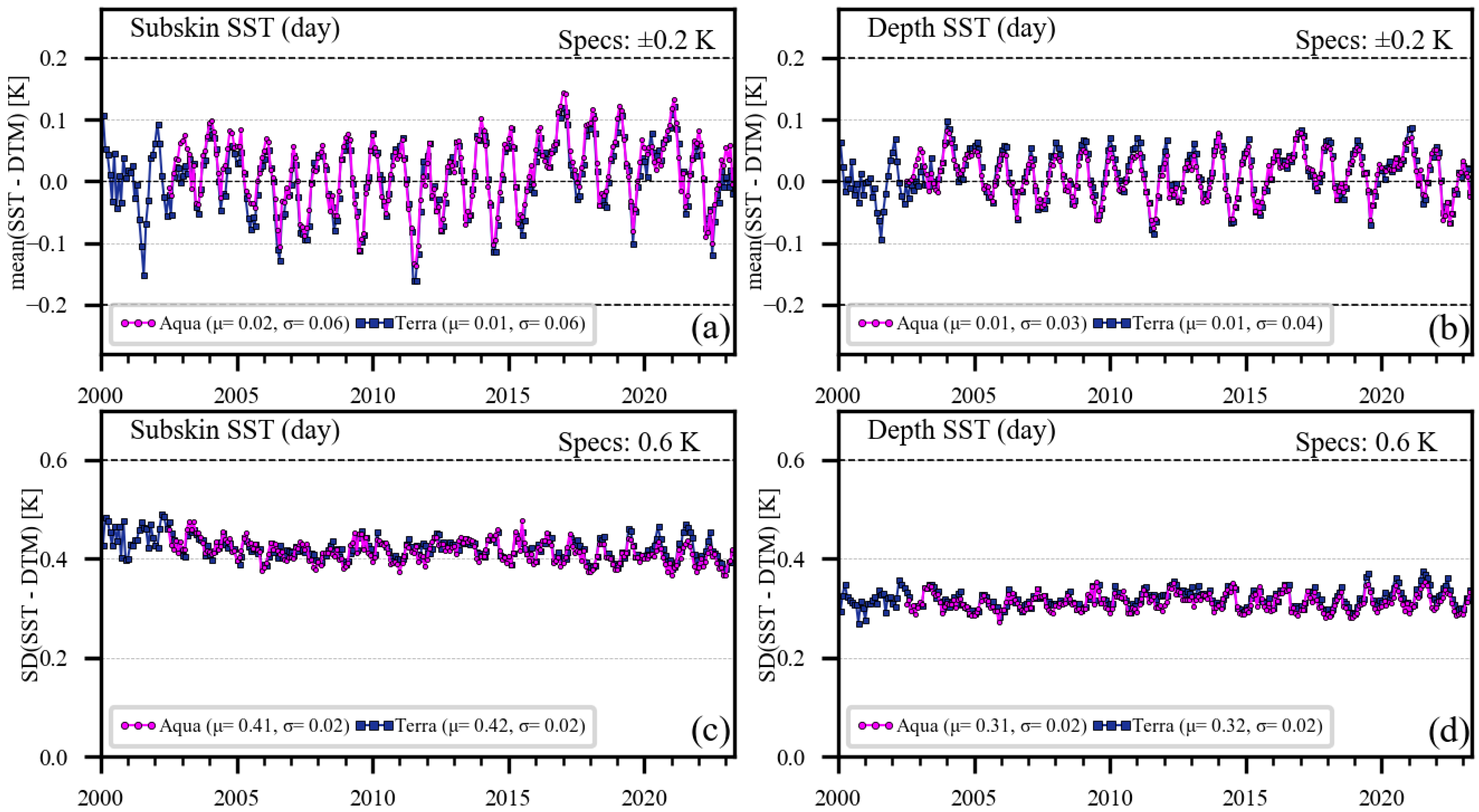
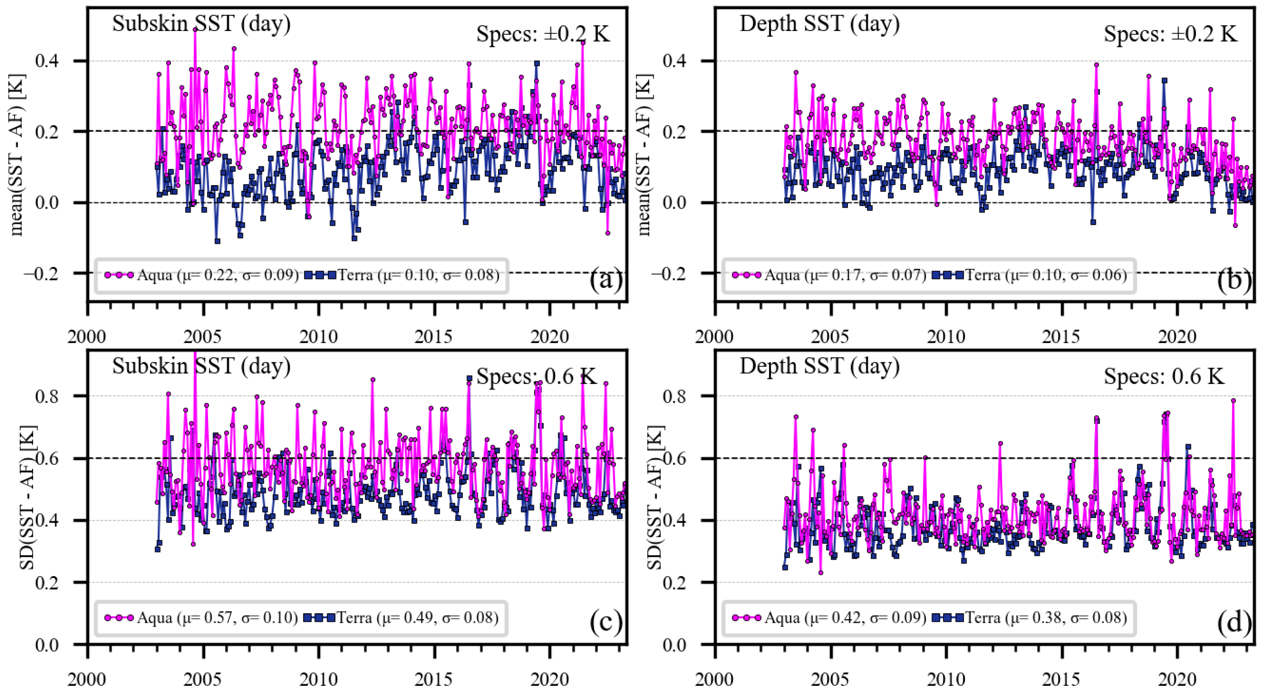
Figure 6 shows the corresponding daytime SST validation statistics against DTMs.
The requirements for accuracy and precision continue to be met for the daytime SST, albeit with a narrower margin. Seasonal variations in accuracy are now seen, with an amplitude of ~±0.1 K for ‘subskin’ and ~±0.07 K for ‘depth’ SSTs. In [
1], such seasonal variations in the VIIRS accuracy were attributed to the space/time temperature difference between the skin SST and temperature at ~0.2–1.0 m measured by DTMs. If this hypothesis were correct, then such seasonal variations would be expected to be larger for Aqua and smaller for Terra, which have very different LEXTs (1:30 p.m. vs. 10:30 a.m.). However, the two curves sit on top of each other. To further rule out the skin-depth thermocline as the underlying reason, we performed an experiment where the Aqua MODIS nighttime SST record was reprocessed using the daytime SST algorithm given by Equation (2). The same seasonal bias was observed as during the daytime, suggesting that a different physical mechanism may contribute, e.g., some seasonality in the in situ DTM data or atmospheric water vapor and temperature profiles, which affects the daytime split-window NLSST more than at night with the transparent 3.7 µm band. At the time of writing, we are unable to identify a direct link between the seasonal daytime SST biases and the atmospheric water vapor. More analyses are needed to explain this seasonality. The answer to this question is important. If there are limitations to the atmospheric correction with the split-window NLSST algorithm, then it should be revisited.
Turning to the precision, the daytime ‘subskin’ standard deviations of ~0.41–0.42 K are degraded from their nighttime counterparts, ~0.33 K, as expected. This is likely due to a combination of the degraded performance of the daytime split-window NLSST, due to the lack of the transparent MWIR band 20 centered at 3.7 µm, and the increased and more variable diurnal stratification of the upper ocean during the daytime. Consistent with the nighttime validation, daytime ‘depth’ SSTs show improved precision (0.31–0.32 K), compared to ‘subskin’ SSTs (0.41–0.42 K). More pronounced seasonality is seen in daytime standard deviations compared to their nighttime counterparts in
Figure 5.
Table 3 summarizes the MODIS RAN1 validation statistics against DTMs for one full year of data (2019).
Figure 5 and
Figure 6 suggest that the accuracy and precision have been stable over time, thus adding confidence that one year is representative of the full Aqua and Terra missions. The year 2019 was chosen, because the Aqua and Terra orbits remained stable, and two ACSPO VIIRS SSTs (from NPP and N20 RAN3) were available for comparison. The year 2019 was also the least affected by the anomalies in drifter data (note the ~0.05 K warm drifter SST bias from 2012–2016 manifested as a negative plateau in the MODIS time series in
Figure 5a,b).
To put the MODIS RAN1 in the context of other available similar products,
Table 3 lists the performance statistics for the VIIRS RAN3 [
1] and NASA R2019 MODIS data [
10,
11]. For the R2019, all pixels with QLs = 4 and 5 are included. This criterion results in a comparable fraction of clear-sky pixels between the ACSPO and NASA products. Excluding QL = 4 pixels improves the NASA validation metrics, but results in a significantly reduced clear-sky domain (by >30%; e.g., all pixels with VZA > 55° are flagged as QL = 4 in the NASA product, in contrast to ACSPO, where QL = 5 retrievals are made in a full sensor swath). Note also that the NASA product reports ‘skin’ SSTs (calculated by subtracting 0.17 K from the regressions trained against DTMs, P. Minnett, K. Kilpatrick, 2023, personal communication). For consistency with the ACSPO ‘subskin’ SSTs, +0.17 K was added to all NASA SSTs.
The RAN1 ‘subskin’ and ‘depth’ SSTs accuracies and precisions are largely consistent between Terra and Aqua. The precision of the ACSPO ‘depth’ SST is improved over the ‘subskin’ (by ~0.05 K at night and by ~0.10 K during the day). The corresponding standard deviations are inferior compared to VIIRS (by ~0.02 K at night and ~0.05 K during the day), presumably due to the use of the M14 band centered at 8.6 µm in the VIIRS retrievals. This band has a lower impact at night, due to a dominant contribution from the MWIR 3.7 µm band. The CSRs are largely consistent across all ACSPO VIIRS and MODIS products. (Recall that the CSR is defined as the ratio of the SST pixels to all ice-free ocean pixels measured by the sensor and serves as a measure of the efficiency of the clear-sky mask). The global coverage (actual area covered by SSTs) is significantly greater for VIIRS compared to MODIS, due to the considerably wider swath (3060 km vs. 2330 km). The wider swath and higher resolution of VIIRS results in about ×3 more satellite pixels, compared to MODIS.
The RAN1 performance is improved over that of R2019. At night, the ACSPO ‘subskin’ standard deviations are ~0.33 K vs. ~0.40 K for NASA. The RSD margin of improvement is narrower, 0.26 K vs. 0.28 K. The corresponding daytime metrics are 0.42 vs. 0.47–0.50 K for the conventional standard deviation, and 0.35–0.37 vs. 0.39–0.43 K for the RSD.
Subtracting the SSES bias (equivalent to obtaining ‘depth’ SST in ACSPO) statistically significantly improves the ACSPO standard deviations and RSDs but has little effect on the NASA statistics, in part due to the not very effective choice of scale factor (0.16 K) in the ‘sses_bias’ field in the NASA files. Recall that as per the GDS2 standards, this variable is stored as a signed eight-bit integer with an associated offset and scale factor. The scale factor determines the quantization of the ‘sses_bias’ variable, and 0.16 K is too large. In the ACSPO files, the SSES bias scale factor is 0.016 K. Because of the differences in the SSES algorithms and numerical implementations, the margin in the performance metrics between the ACSPO ‘depth’ SSTs and the SSES-bias-corrected NASA SSTs is wider compared with the ‘subskin’ SST.
At night, the ACSPO NOBSs (number of matchups with DTMs) are larger than NASA NOBSs: 20.6 M (Million) vs. 17.7 M for Terra and 19.1 M vs. 16.3 M for Aqua. During the daytime, ACSPO has fewer matchups: 19.3 M vs. 22.6 M for Terra and 20.4 M vs. 22.6 M for Aqua. Adding up the night and day NOBSs, one obtains the following ACSPO vs. NASA statistics: 39.9 M vs. 40.3 M for Terra, and 39.5 vs. 39.9 M for Aqua, which are within 1% of each other. ACSPO day/night NOBSs are more closely balanced than NASA, which may be due to different definitions of day and night in ACSPO and NASA processing.
Additional analyses in
Appendix A provide validation against Argo Floats (AFs). These are largely consistent with the DTM analyses above but being fully independent, provide an additional important consistency check.
ACSPO CSRs are larger than NASA CSRs at night (20.6% vs. 17.7% for Terra and 19.1% vs. 16.3% for Aqua), and smaller during the daytime (19.3% vs. 22.6% for Terra and 20.4% vs. 22.6% for Aqua). The ACSPO mask thus appears more liberal than NASA at night and more stringent during the daytime.
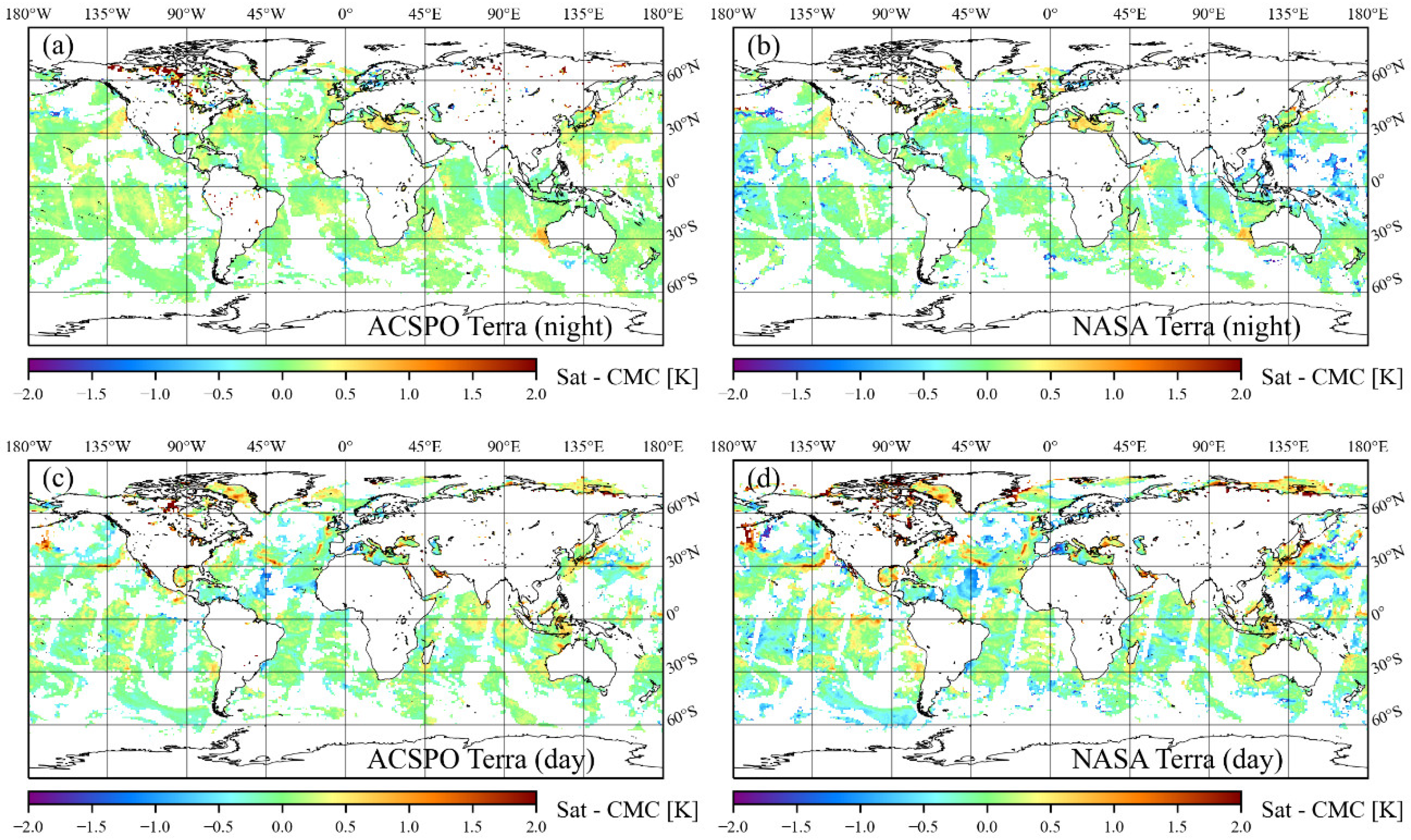
Figure 7 shows 24 h aggregated global maps of the Terra ACSPO and NASA SST biases against the gap-free Canadian Meteorological Centre (CMC) L4 foundation SST [
37] for both night and day, for one representative day of data, 1 August 2019. Bluish spots, seen in both products, suggest residual cloud or aerosol leakages. Those are more frequent and pronounced in the NASA SST. Terra was chosen for this demonstration because of the suppressed diurnal signal and, hence, the expected closer proximity of satellite SST to the CMC L4 foundation SST. The Aqua patterns are similar. Apart from residual cloud leakage, the agreement between the ACSPO and NASA SSTs is quite close, with no systematic regional differences visible in
Figure 7. Both the ACSPO and NASA daytime SSTs exhibit cold biases in the North Atlantic between 10°N and 30°N, likely due to dust aerosols originating from the Sahara Desert in Northern Africa.
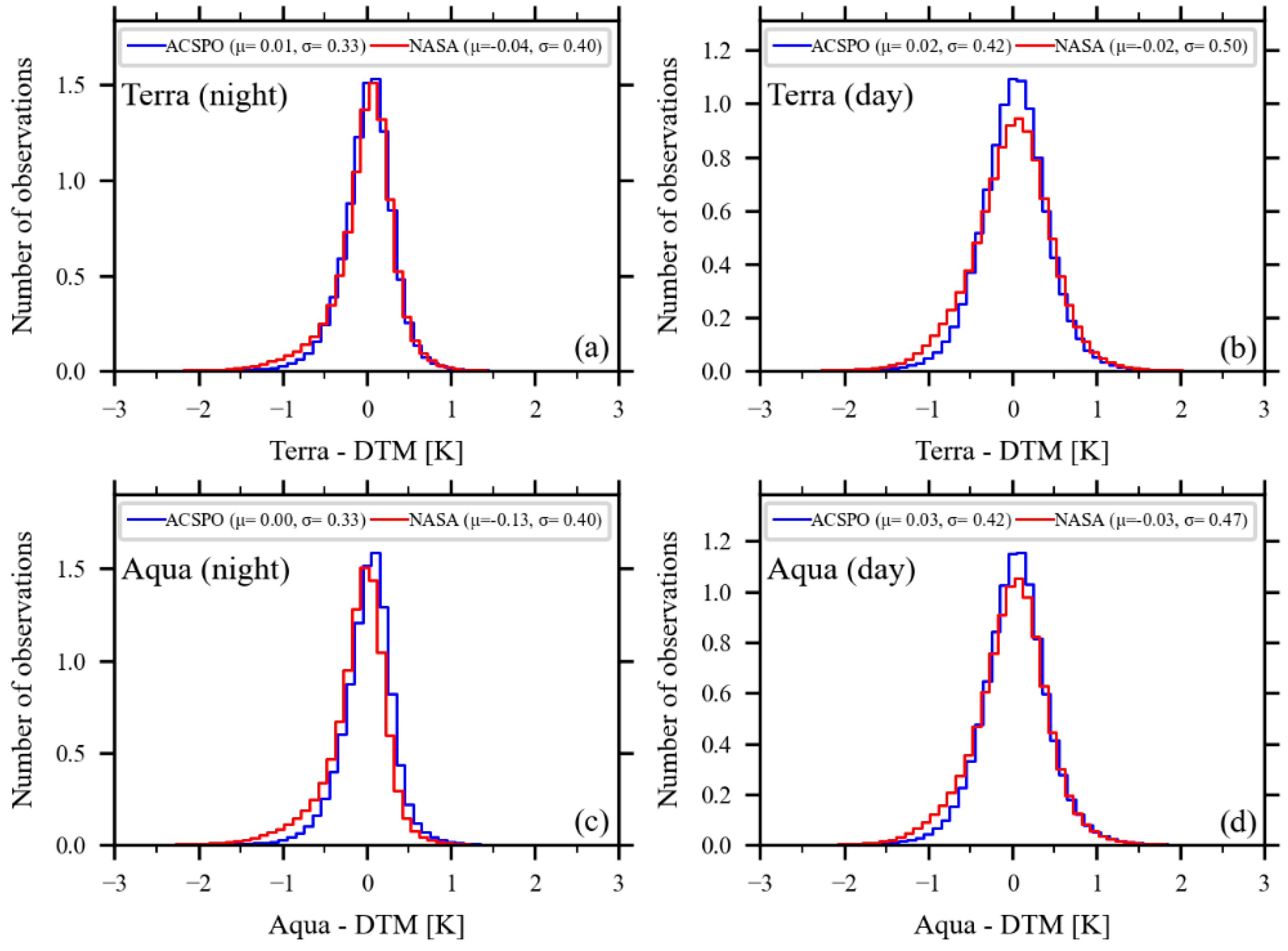
Figure 8 compares ACSPO and NASA histograms of bias with respect to DTMs for the one-year period analyzed in
Table 3. The NASA histograms are less symmetric and show a more pronounced cold tail. This is consistent with the higher NASA standard deviations and RSDs shown in
Table 3 (and a wider margin between those), and the increased residual cloud leakage seen in
Figure 7.
4.2. Long-Term Stability
Estimating the stability of the satellite SST via a comparison with the in situ SST is a nontrivial task due to uncertainties inherent in the in situ data themselves. Both drifters and TMs have their pros and cons when it comes to stability estimation. It may not be easy to separate drift in satellite SSTs from regional biases modulated by changes in the drifter geographical distribution. An improved accuracy, stable geographical distribution, and reduced seasonality near the equator make TMs attractive for studying the long-term stability of satellite SSTs, as has been explored in the (A)ATSR Reprocessing for Clime (ARC) and JPSS VIIRS RAN3 [
1,
36]. However, TMs are less numerous than drifters, leading to noisier validation statistics. The deeper TM measurements (~1 m) also pose a challenge for validation during the daytime, when a significant diurnal thermocline may be present. Another challenge with using TMs is the lack of atmospherically transparent MWIR bands during the daytime, making satellite SST retrieval through the humid tropical atmosphere less accurate. For the reasons listed above, we present analyses of the long-term stability of the MODIS RAN1 SST using both DTMs and TMs as references. We omit AFs from the stability analysis for two reasons: (1) there were very few AF platforms in the early 2000s, and their fleet was rapidly changing; and (2) the depth of their shallowest SST measurements evolved over time. Since 2013, some AFs have started to report near-surface SSTs as shallow as 0.2 m, compared to the typical ~5 m depth reported in the 2000s [
38]. The challenge of the varying AF measurement depth can be overcome by using the SST measurement nearest to 5 m from a given AF profile. However, the current iQuam v2.10 designed in 2008 selects the shallowest high-quality SST from a given profile. The NOAA SST team is exploring the inclusion of the measurement closest to a chosen nominal depth of ~5 m, in addition to keeping the shallowest AF measurement.
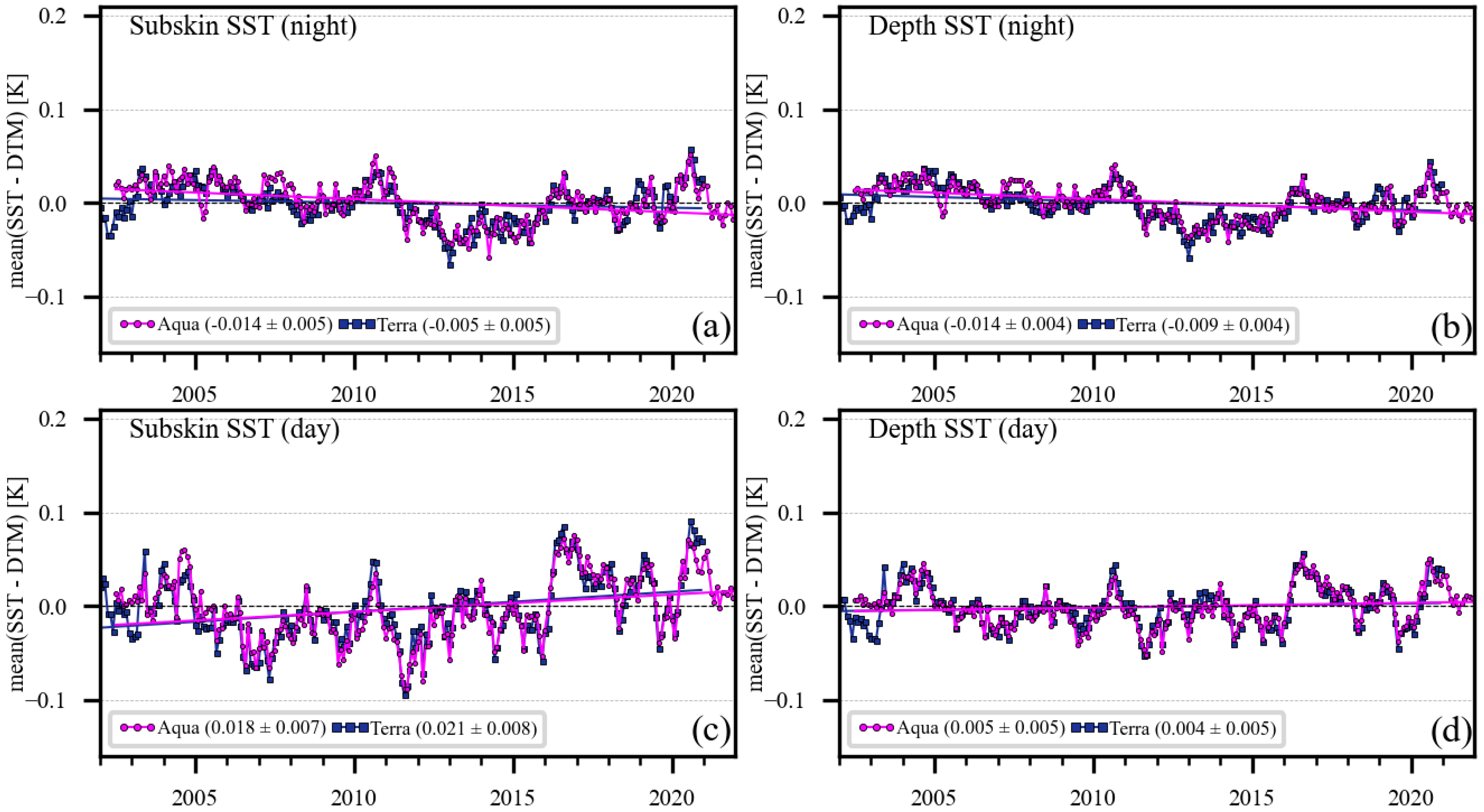
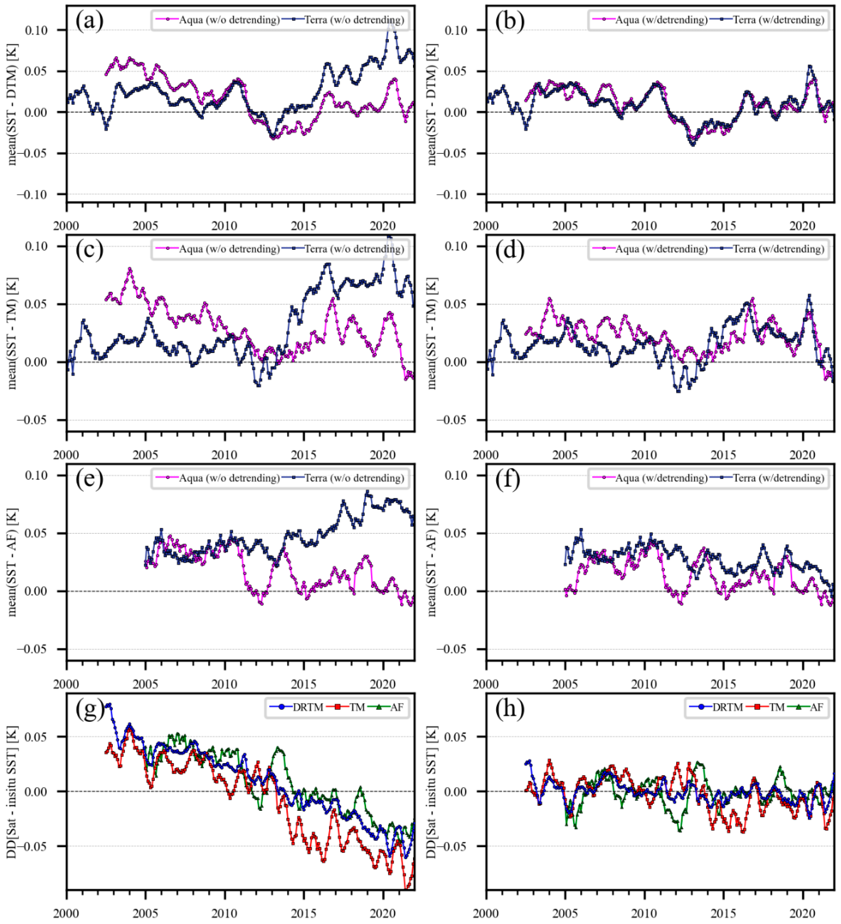
Figure 9 shows the time series of the ΔT
S = MODIS RAN1 − DTM SST mean bias for both ‘subskin’ and ‘depth’ SSTs during the day and night. Linear trends obtained using least square fits are also overlaid. Note that
Figure 9 and all further stability estimates in this section only employ time periods with stable LEXTs (1 January 2002–31 December 2020 for Terra and 4 July 2002–31 December 2021 for Aqua) to minimize the effect of the variable local observation time.
Figure 9a,b shows that the drift is ~−0.014 K/decade for Aqua (for both ‘subskin’ and ‘depth’ ΔT
Ss) and ~−0.005 and −0.009 K/decade for Terra ‘subskin’ and ‘depth’ SSTs, respectively. We attribute (at least partially) the slightly negative drifts in the nighttime ΔT
Ss, consistent between Aqua and Terra, to a systematic ~0.05 K warm bias in iQuam drifter data between 2012 and 2016 (also observed in ACSPO VIIRS SST [
1]).
Figure 9c,d shows the corresponding daytime ΔT
S. For Aqua, the drifts are +0.018 and +0.005 K/decade for the ‘subskin’ and ‘depth’ SSTs, respectively. For Terra, they are +0.021 and +0.004 K/decade for the ‘subskin’ and ‘depth’ SSTs, respectively.
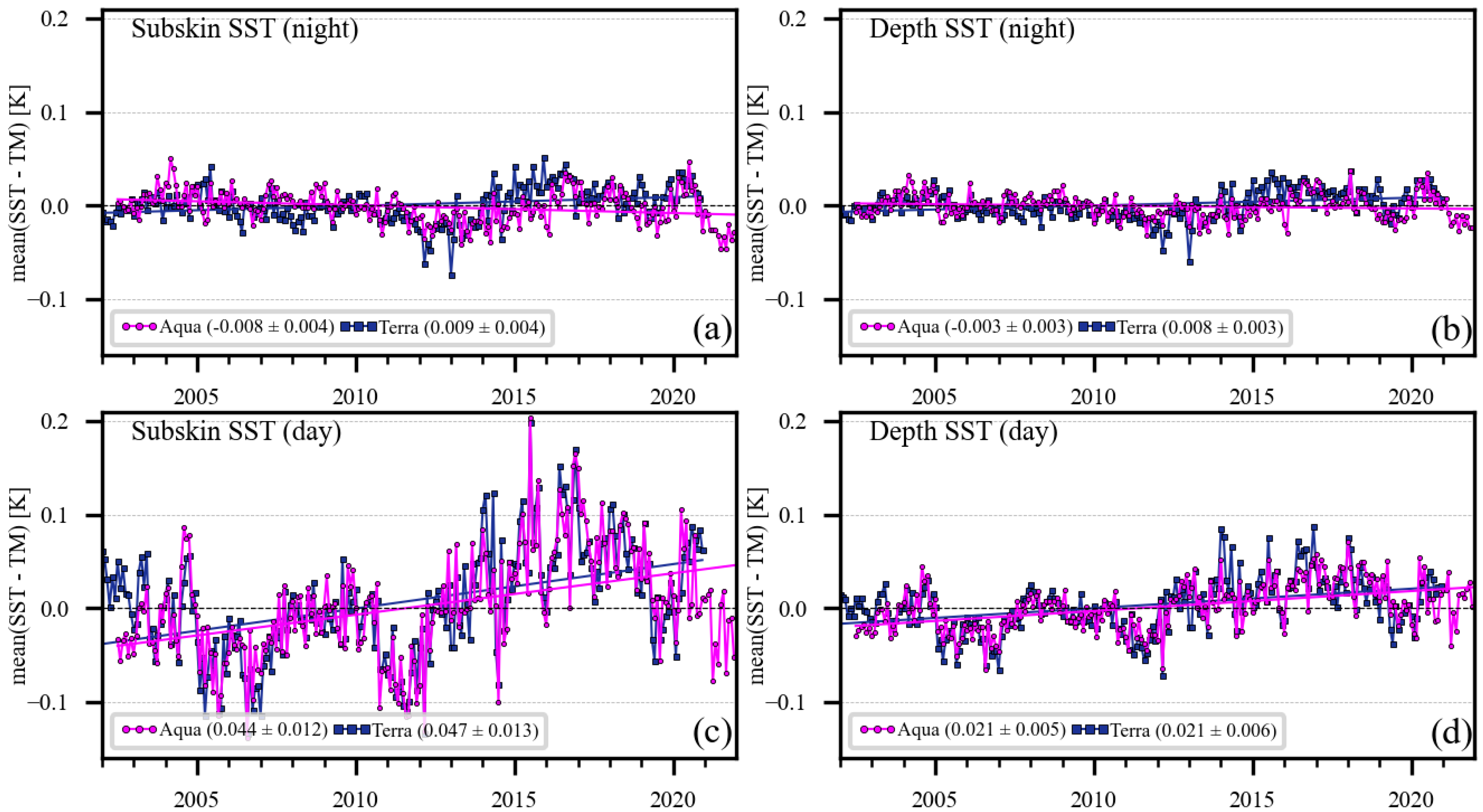
Figure 10 shows the same stability analysis as in
Figure 9 but uses TMs as a reference.
Figure 10a,b shows that both Terra and Aqua nighttime ΔT
Ss have remained very stable when compared to the TMs, with estimated drift magnitudes of below 0.01 K/decade for both the ‘subskin’ and ‘depth’ SSTs. The small nighttime SST trends vs. TMs are counter-directed for Aqua (negative) and Terra (positive), in contrast to the trends against the DTMs (
Figure 9a,b) which are all negative.
Figure 10c,d shows the daytime results. While still meeting the target stability of 0.05 K/decade, the estimated daytime drifts vs. TMs are all positive and are considerably larger compared to the nighttime counterparts (~+0.045 vs. ~±0.01 K/decade for ‘subskin’ and 0.021 vs. ~0 K/decade for ‘depth’). The estimated daytime drifts against TMs are significantly larger than those against DTMs (
Figure 9c,d), possibly due to the stronger diurnal thermocline at TM SST depths (~1 m) and the absence of atmospherically transparent MWIR channels in the daytime satellite SST algorithm. Furthermore, the TM daytime results after 2011 show increased noise, likely due to the significantly decreased number of TM matchups after 2011 (cf.
Figure 4b).
Estimates of the ACSPO MODIS RAN1 daytime and nighttime ΔT
S trends are summarized in
Table 4 against both DTMs (from
Figure 9) and TMs (from
Figure 10).
All ΔT
Ss meet the target stability of ±0.05 K/decade. At night, analyses vs. TMs are deemed more reliable due to the 2012–2016 systematic cold bias against DTM SSTs, which is common to both Aqua and Terra MODISs (as well as NPP/N20 VIIRS SSTs [
1]). For daytime SSTs, on the other hand, the estimates against DTMs appear to be more realistic, due to the significant noise in the ΔT
S time series vs. TMs in
Figure 10c,d. For the remainder of this paper, the reported stability estimates for night SST are based on the TMs, whereas for the day SST, they are based on the DTMs. With this choice, both day and night Aqua/Terra ‘depth’, as well as the night ‘subskin’ trends, are well within ±0.01 K/decade. The daytime ‘subskin’ SST drift is largest, on an order of +0.02 K/decade for both Terra and Aqua. Considerably reduced drift in the daytime ‘depth’ SST (computed using piecewise regression) compared to the ‘subskin’ SST (computed using global regression) may be due to an interplay between seasonal biases (which are reduced in the ‘depth’ SST) and the evolving DTM global geographical distribution.
6. Conclusions
A global 1 km resolution 1st MODIS Reanalysis (RAN1) SST dataset was produced at NOAA using its enterprise Advanced Clear Sky Processor for Ocean (ACSPO) version 2.80 system, for the full Terra (24 February 2000—on) and Aqua (4 July 2002—on) missions. The MODIS RAN1 complements two other existing ACSPO v2.80 RANs: from VIIRSs flown onboard 3 JPSS satellites (NPP from February 2012—on; N20 from January 2018—on, and N21 from March 2023—on), and AVHRR FRACs flown onboard 3 Metop-FG satellites -A (December 2006–November 2021), -B (October 2012—on), and -C (December 2018—on) [
1,
2]. Two SST products are available in ACSPO v2.80 files, ‘subskin’ and ‘depth’. The locations and intensity of thermal fronts are also reported.
A comparison of MODIS SSTs with quality-controlled in situ SSTs from drifters and tropical moorings (DTMs) and Argo floats (AFs) from the NOAA iQuam system shows that MODIS RAN1 SSTs are of high and uniform quality, and consistent across Terra and Aqua. They meet the NOAA JPSS specs for accuracy (global mean bias with respect DTM < ±0.2 K) and precision (corresponding global standard deviation < 0.6 K), and often exceed them by a wide margin. This performance is achieved in a clear-sky domain (fraction of clear ice-free ocean pixels in sensor view) of 19.1–20.6%. Estimates of the Δ
TS =
TSAT −
TIS stability vs. the in situ SST were performed. At night, the Aqua and Terra SSTs agree very closely. The corresponding drifts relative to the TMs do not exceed ±0.01 K/decade, for both the ‘subskin’ and ‘depth’ SSTs. During the daytime, drifts in the ‘depth’ SSTs are again within ±0.01 K/decade, whereas for the ‘subskin’ SST a positive drift of ~+0.02 K/decade is seen for both Aqua and Terra. All estimates are well within the (A)ATSR Reprocessing for Climate (ARC) project target stability of 0.05 K/decade [
36].
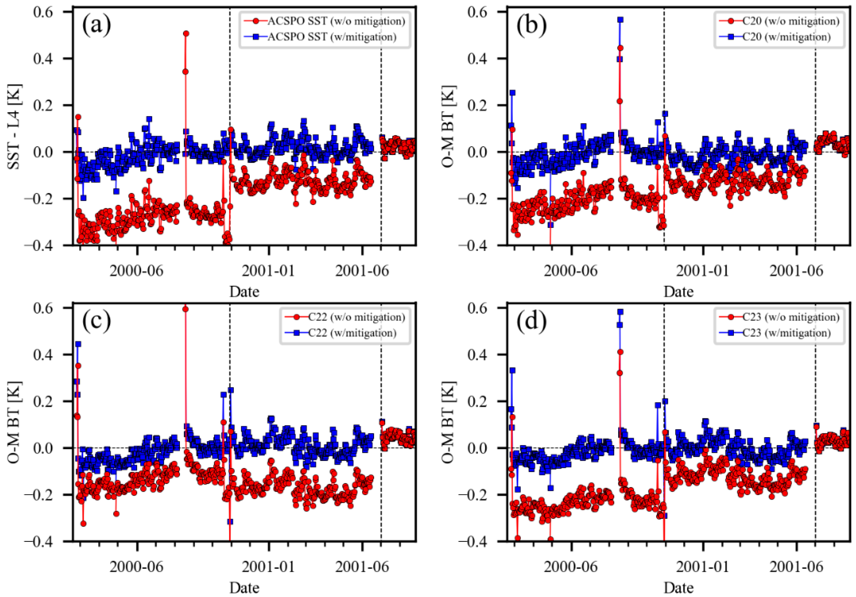
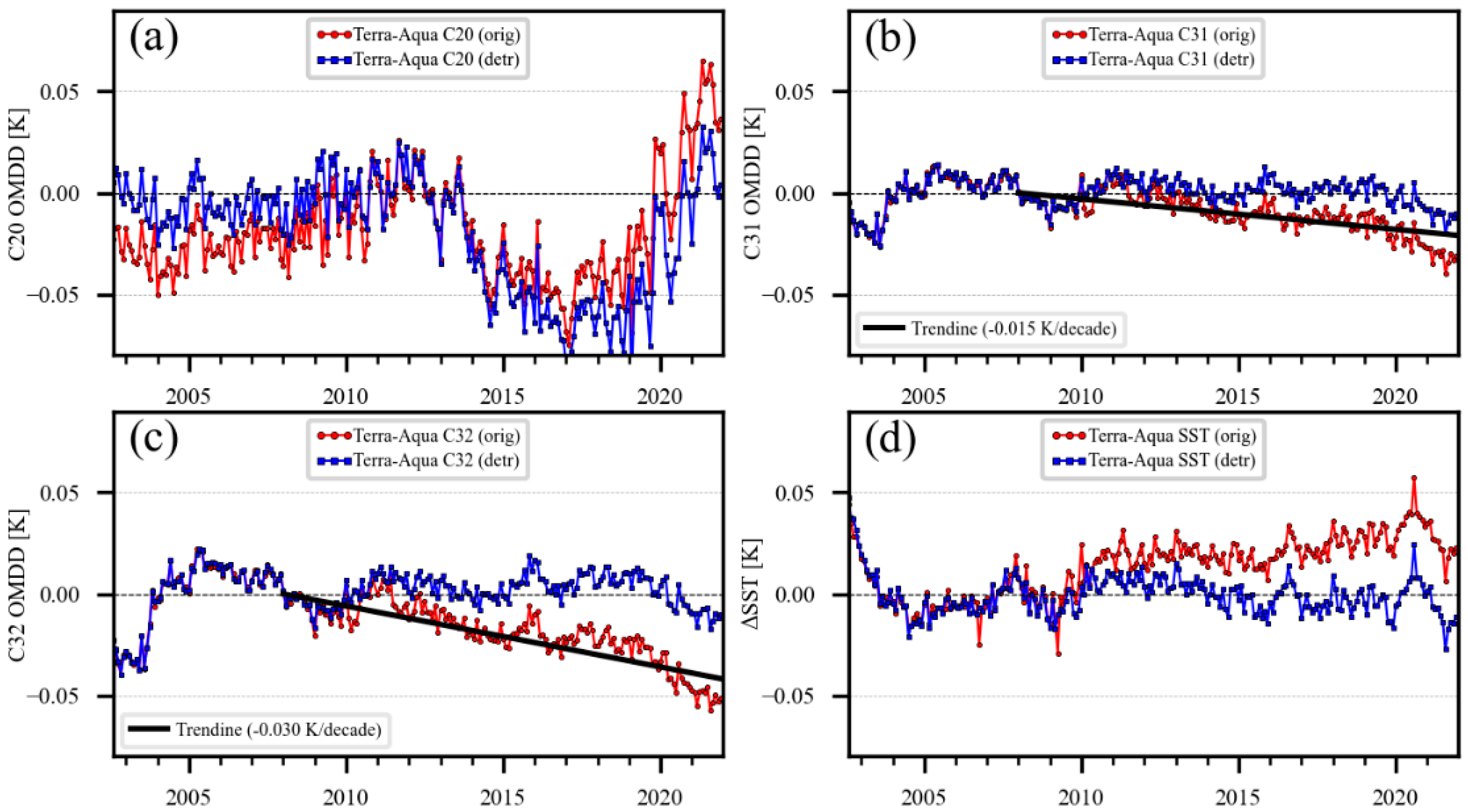
Achieving these high standards of performance required some corrections and adjustments to the MODIS brightness temperatures (BTs), in particular, for Terra, which were addressed in RAN1. Two steps in mid-wave infrared (MWIR) BTs in bands 20, 22, and 23, were related to changes in the Terra MODIS operating configuration. If not accounted for, these BT steps result in three epochs of nighttime SSTs, each of which is stable, but with ~0.1 K inconsistencies between configuration changes. The steps in Terra MODIS MWIR calibration and their effects on nighttime SSTs were previously reported in [
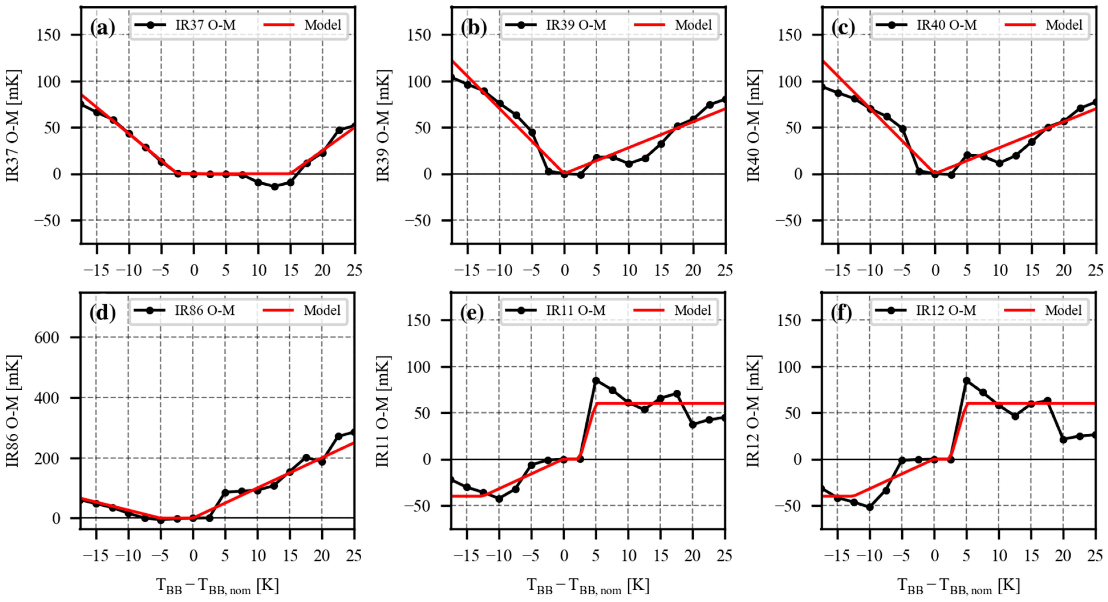
8]. The authors mitigated those by training separate SST retrieval coefficients for each epoch. This approach may not be optimal due to the relative scarcity of in situ training data in the early 2000s and the short durations of the first two epochs (less than a year each). In MODIS RAN1, those were mitigated by estimating the BT discontinuities from the time series of the global mean observed minus modeled (‘O-M’) BT biases, and those offsets were used to debias the Terra MODIS L1b BTs in MWIR bands 20, 22, and 23.
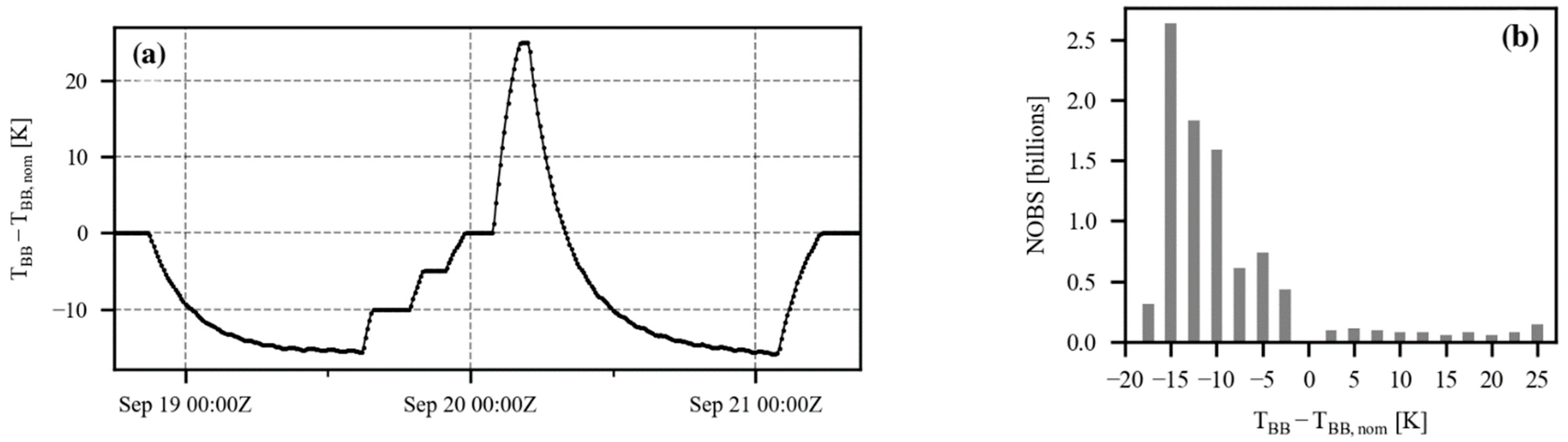
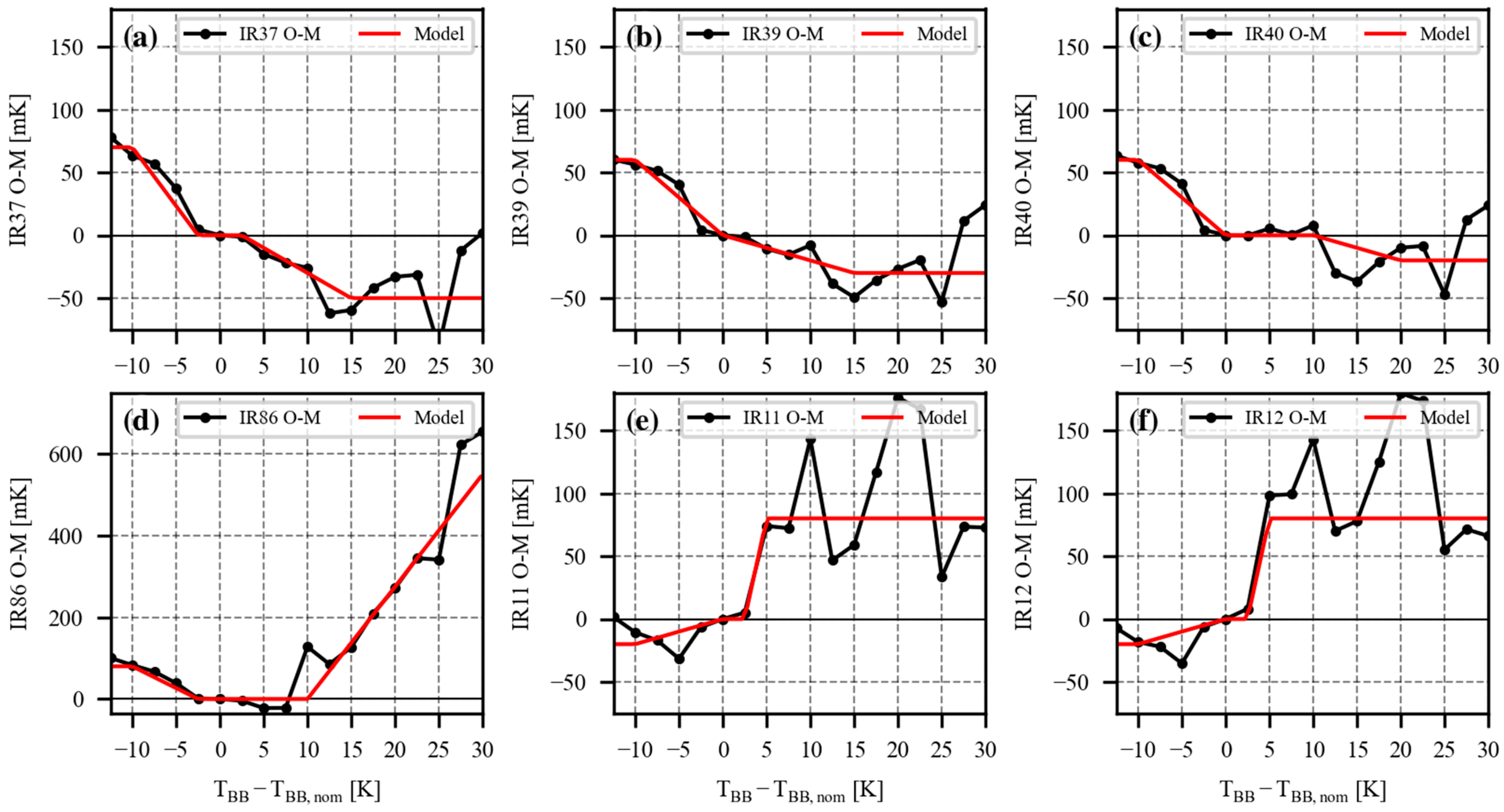
During the early evaluation, we observed artifacts in the Terra nighttime SSTs, concurrent with changes in the MODIS nominal BBT during quarterly warm-up cool-down (WUCD) events, when a positive ~0.1 K global daily mean biases were observed (
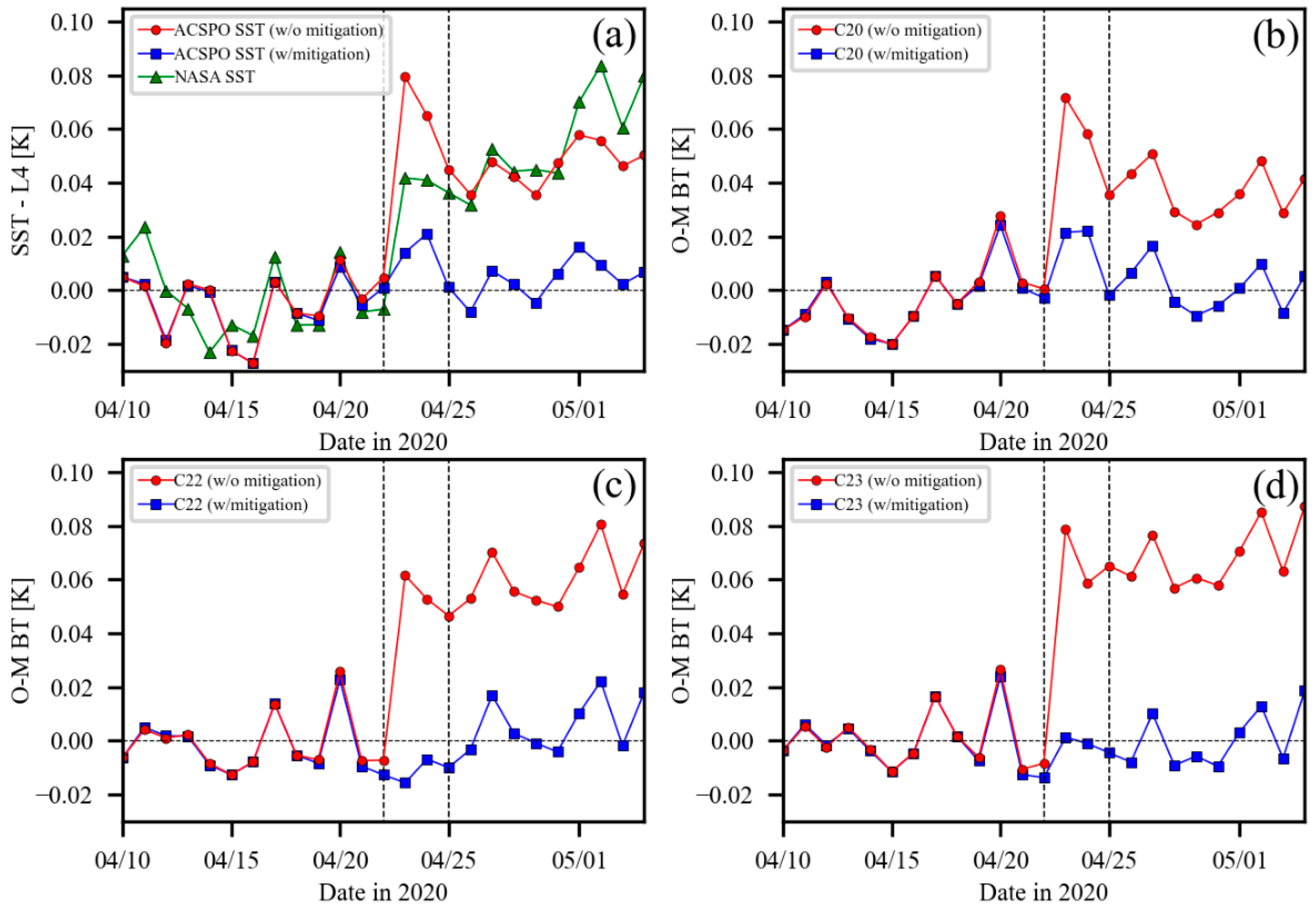
Appendix B). In MODIS RAN1, these steps were mitigated by computing the ‘O-M’ BT bias dependency on blackbody temperature (BBT) anomalies (deviation from the nominal temperature). Estimated corrections were applied to Terra MODIS thermal emissive bands (TEBs). The MWIR bands are more affected than the longwave infrared (LWIR) bands, which explains the much smaller SST artifacts during the daytime. We also identified and corrected discontinuities in the MWIR BTs, when the Terra MODIS nominal BBT changed from 290 to 285 K on 25 April 2020. If not accounted for, this step in the BTs results in a positive ~0.05 K step in the nighttime ‘subskin’ SST. We did not observe Aqua MODIS calibration artifacts related to BBT variations during WUCDs.
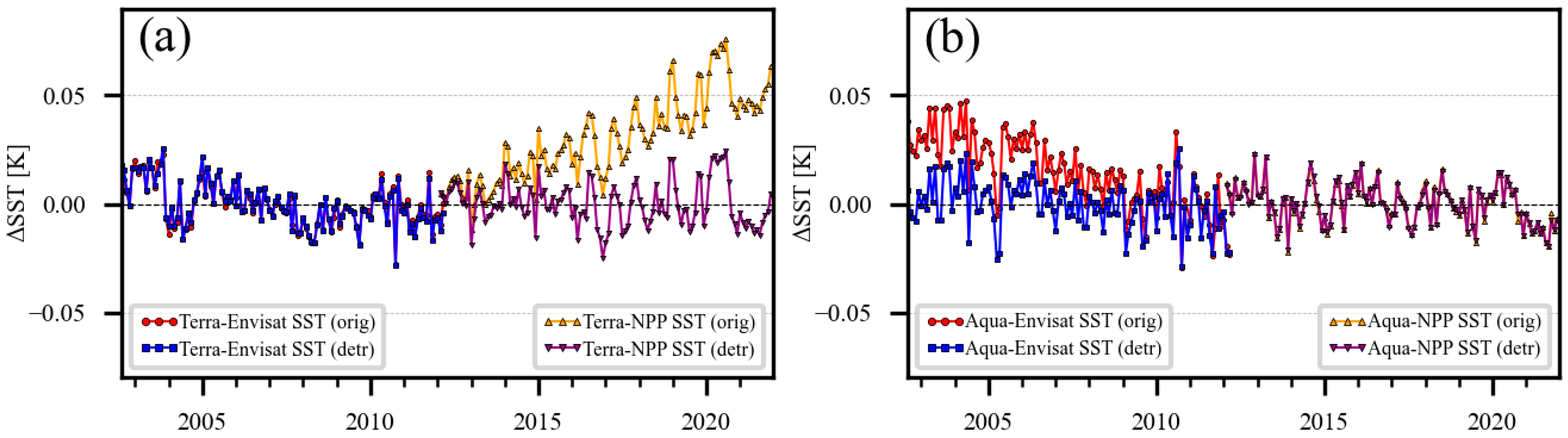
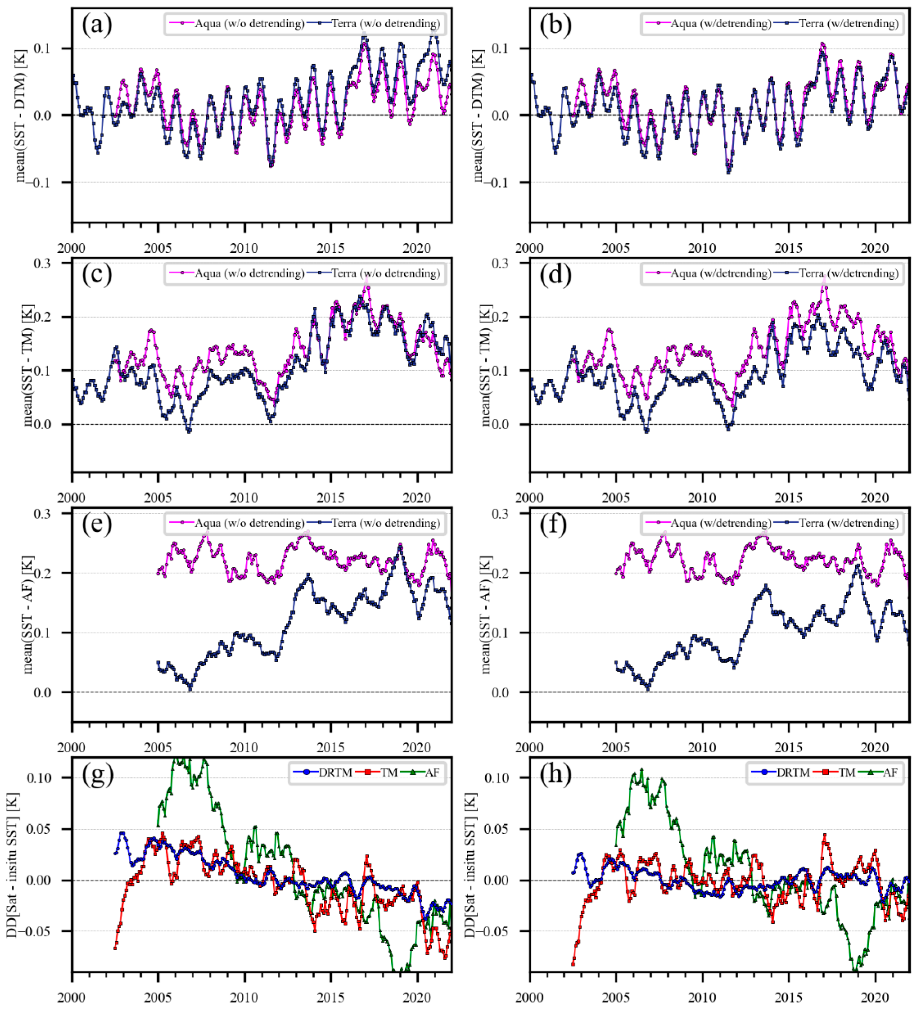
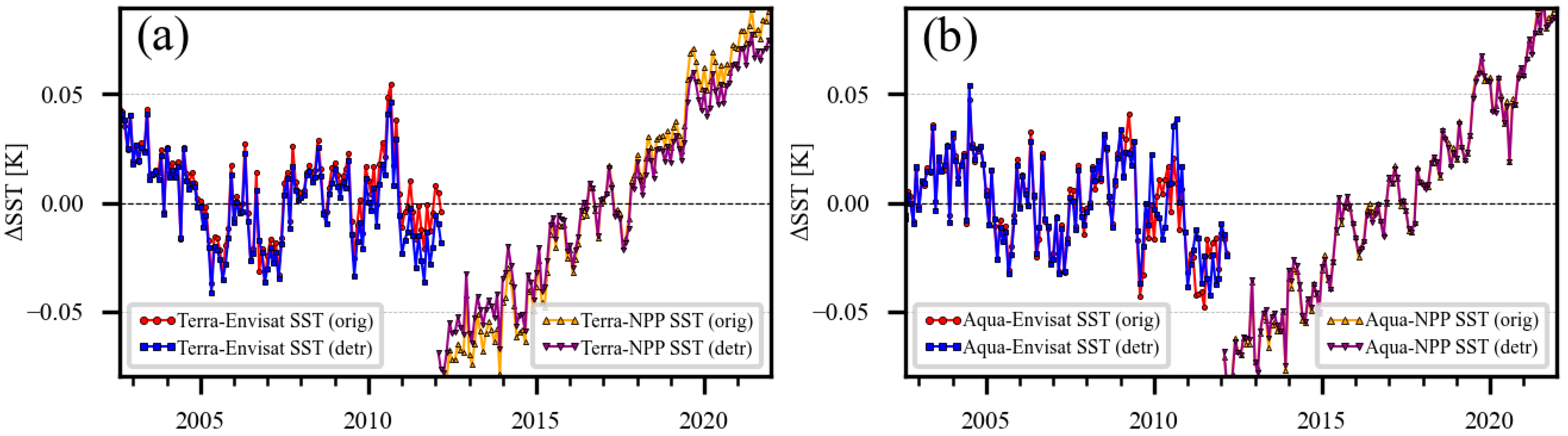
Initial checks of the stability of the MODIS SSTs demonstrated drift on the order of 0.025 K/decade against various in situ SSTs over the course of both Terra and Aqua missions. An analysis of the Aqua and Terra MODIS observed minus modeled (‘O-M’) BTs and cross-comparisons with SST trends enabled us to identify and estimate calibration drifts in MODIS TEBs. We used the estimated drifts to detrend MODIS L1b data and confirmed the improved stability of the ACSPO MODIS RAN1 SST. The presence of the drifts in the original MODIS data and the efficacy of their correction in present work were independently confirmed by comparisons with Envisat AATSR and NPP VIIRS SSTs.
At the time of writing, the complete archive of Terra and Aqua 0.02° Level 3 collated data (L3C; two files per 24 h stratified by day and night) is available at NOAA CoastWatch [
5]. Due to the large data volume, MODIS RAN1 L2P and L3U data have not yet been archived. Archival of the full MODIS RAN1 dataset, including L2P, L3U, and L3C, will be discussed with NASA PO.DAAC and NOAA NCEI. New data are added in ‘science quality’ delayed mode monthly, with a latency of two months (approximate latency of the availability of MERRA atmospheric profiles [
44,
45,
46]). Due to the ongoing degradation of the Terra and Aqua orbits and the associated degradation of the SST data quality, new data are not added in near-real-time. For users interested in near-real-time SST data, we recommend JPSS VIIRS and Metop-FG AVHRR FRAC SST data [
1,
2].
Users interested in a reduced volume, more-information-dense SST data, can use ACSPO 0.02° super-collated family of products from low-Earth-orbiting platforms (L3S-LEO) [
14]. The L3S-LEO family includes three lines. The ‘PM’ line from afternoon orbit satellites (in v2.80, NPP and N20); the ‘AM’ line from mid-morning orbit satellites (in v2.80, Metop-A/B/C). The P.M. and A.M. lines each report two files per 24 h, stratified by the day and nighttime viewing conditions. The daily (DY) product combines data from all available ACSPO L3S-LEO a.m./p.m. data, from both day and night, into a single daily file, with the SST normalized at 1:30 a.m. local time viewing conditions (nighttime P.M. orbit).
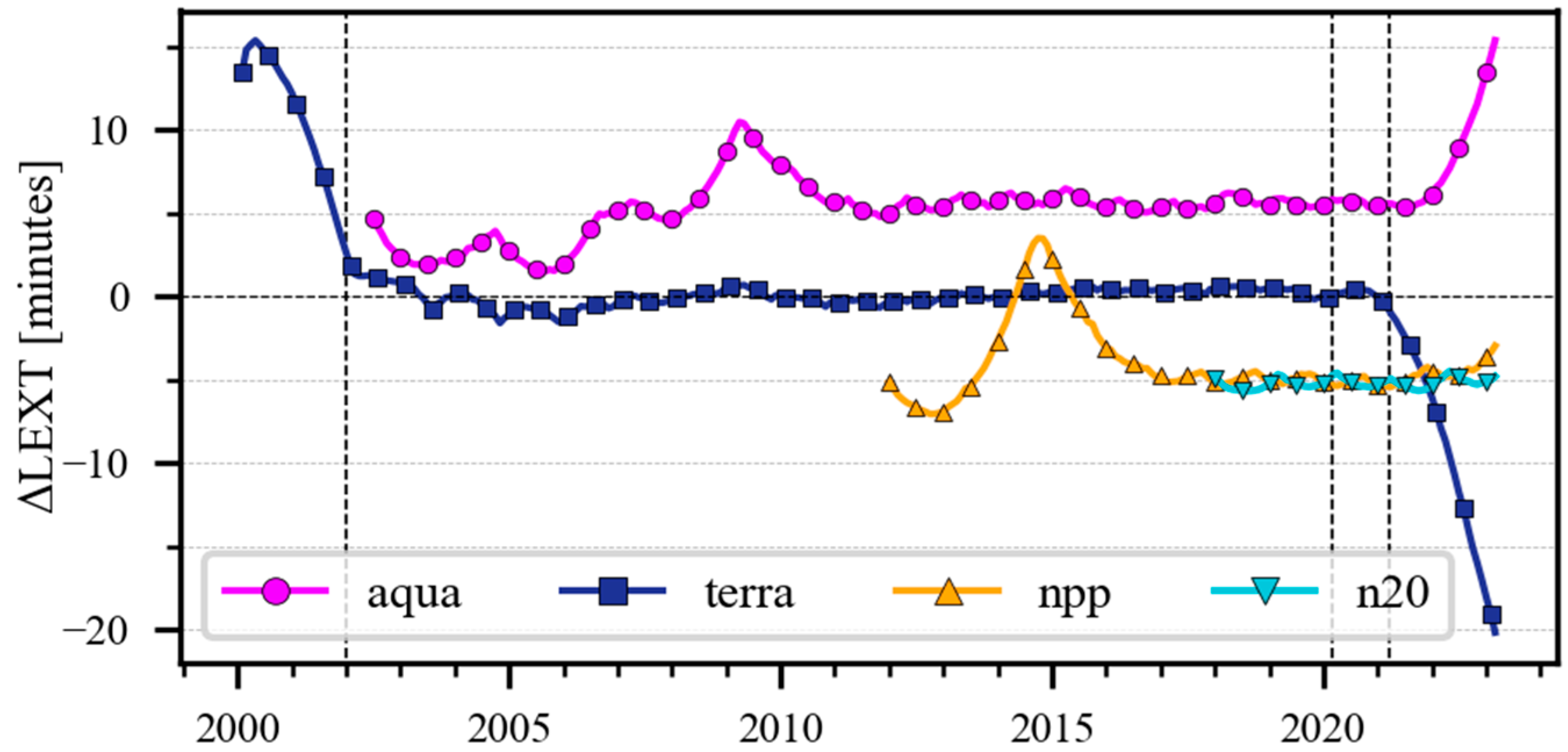
Extending the L3S-LEO-PM time series from February 2012 (earliest NPP VIIRS SST) back to July 2002 (earliest Aqua MODIS SST) was requested by NOAA users and served as the major motivator and driver for MODIS RAN1. Aqua MODIS SSTs are included in L3S-LEO-PM v2.81, an update from v2.80, which only included VIIRS data. Due to its current orbital drift, Aqua SST data are not included in L3S-LEO-PM v2.81 after 31 December 2022 (see
Figure 1). Data from Terra are not included in the A.M. line, due to the significant difference in LEXT (10:30 a.m./p.m.) compared to Metop-FG (9:30 a.m./p.m.). However, Terra SST data are included in the L3S-LEO-DY v2.81 product, and the covered period extends back to 24 February 2000. Due to orbit degradation, Terra is not included in L3S-LEO-DY after 31 December 2021 (see
Figure 1). A complete archive of both the L3S-LEO-PM and L3S-LEO-DY v2.81 products, which include MODIS, is available at NOAA CoastWatch [
14] succeeding the previous v2.80 datasets. Archival of L3S-LEO v2.81 at PO.DAAC is underway.
Future ACSPO MODIS work will include the mitigation of Aqua and Terra orbit drift on the retrieved SSTs. The last (non-collision avoidance) orbit maintenance maneuvers were performed on 27 February 2020 for Terra and on 19 March 2021 for Aqua. Since then, the Aqua and Terra LEXTs have been drifting from their nominal 1:30 a.m./p.m. and 10:30 a.m./p.m. times, respectively. As of the time of writing, the LEXTs have only drifted by about 10 min for Aqua and 20 min for Terra, and the effects on the retrieved SSTs are still relatively small when validated against in situ SSTs (see
Section 4).
Future work will also involve improvements to the ACSPO Clear-Sky Mask (ACSM) to reduce cloud leakage and over-screening and improve the SST algorithms. The ACSPO v2.80 night-time SST algorithm used for RAN1 employs a traditional multi-band NLSST algorithm, which uses one MWIR band (20) at 3.7 µm and two LWIR bands (31 and 32) at 11 and 12 µm, respectively. A similar SST algorithm was used for ACSPO AVHRR FRAC [
2], and a slightly revised algorithm that additionally includes the VIIRS band M14 at 8.6 µm, was used for VIIRS SST retrievals [
1]. The authors of [
8] reported an improved MODIS nighttime SST performance with a MODIS-unique two-band nighttime SST4 algorithm that employs only two MWIR bands (22 and 23) at 3.9 and 4.0 µm. These bands may be additionally explored in future MODIS RANs.


 and
and 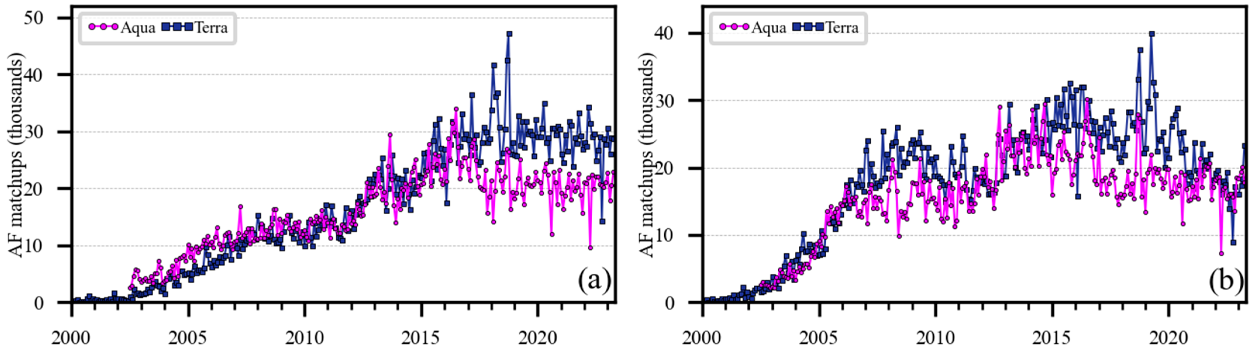
