

VIIRS Edition 1 Cloud Properties for CERES, Part 2: Evaluation with CALIPSO

 ,
,
Abstract
1. Introduction
2. Materials and Methods
2.1. Data
2.1.1. CERES VIIRS Edition 1 Cloud Products
2.1.2. CALIPSO Data
2.2. Comparison Process and Statistics
3. Results
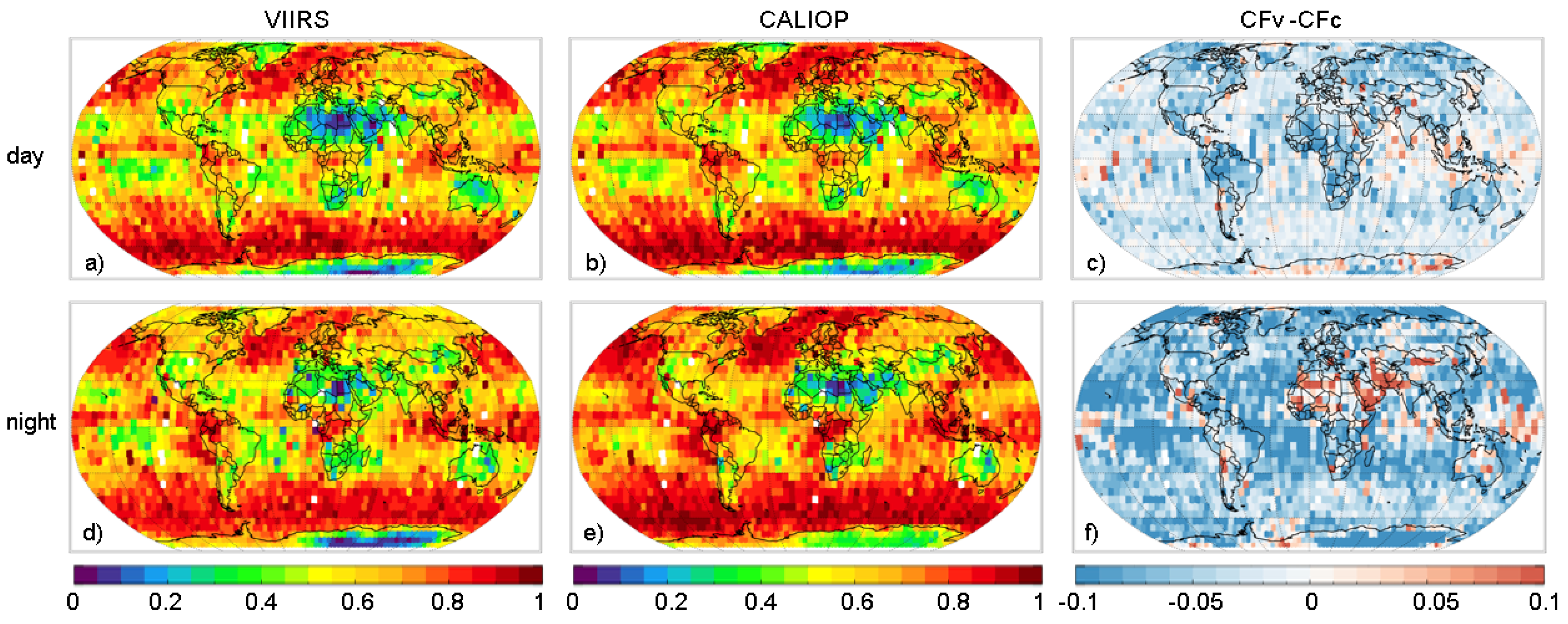
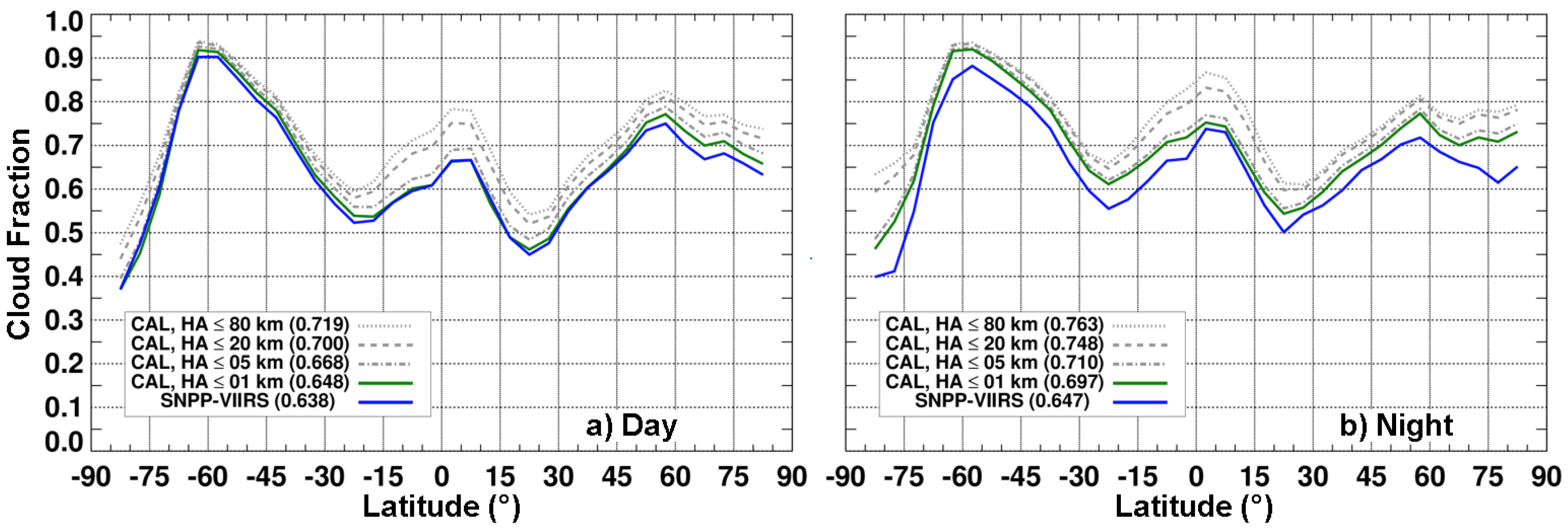
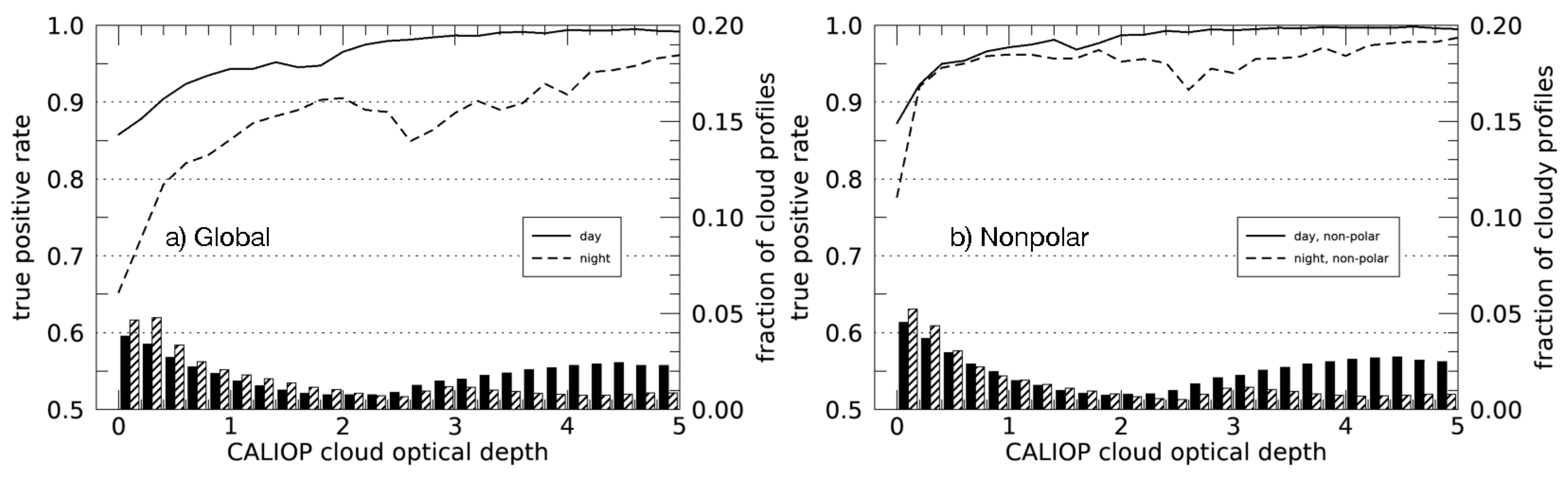
3.1. Cloud Amount
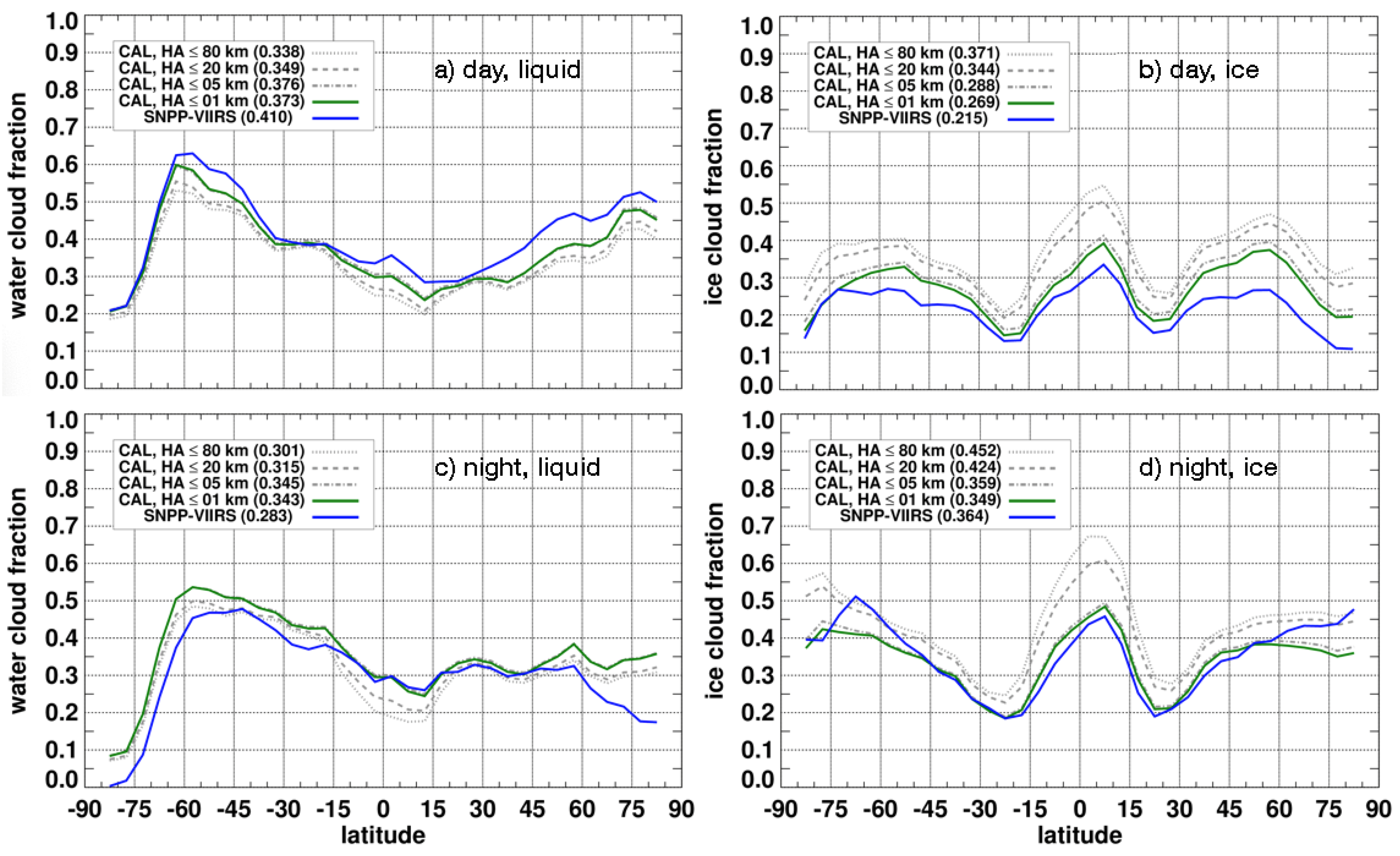
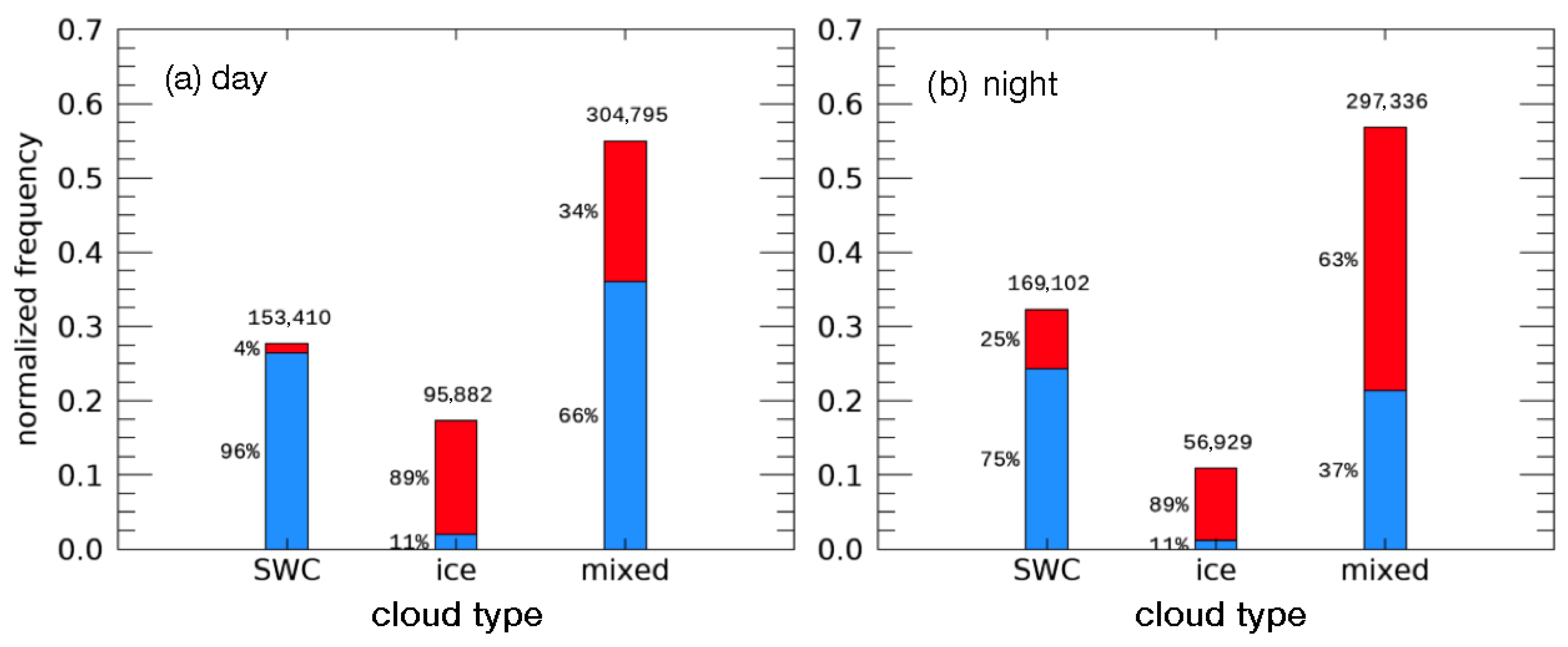
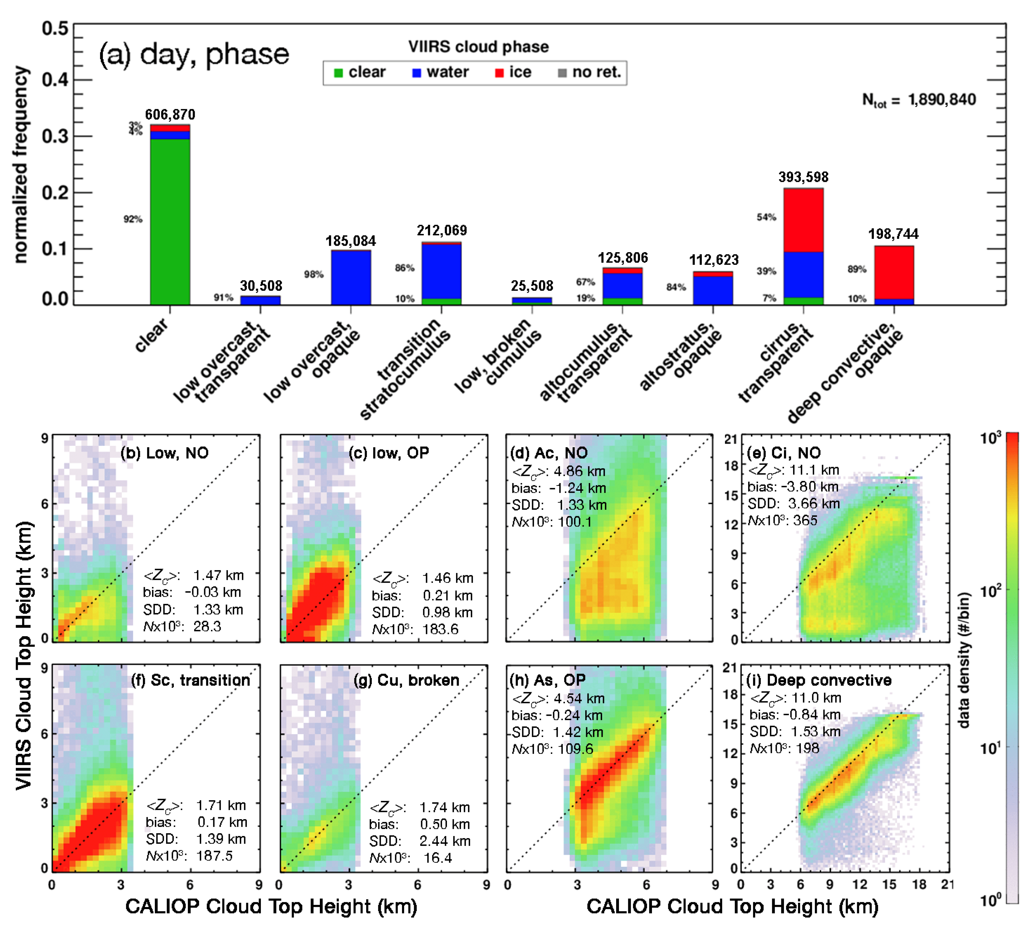
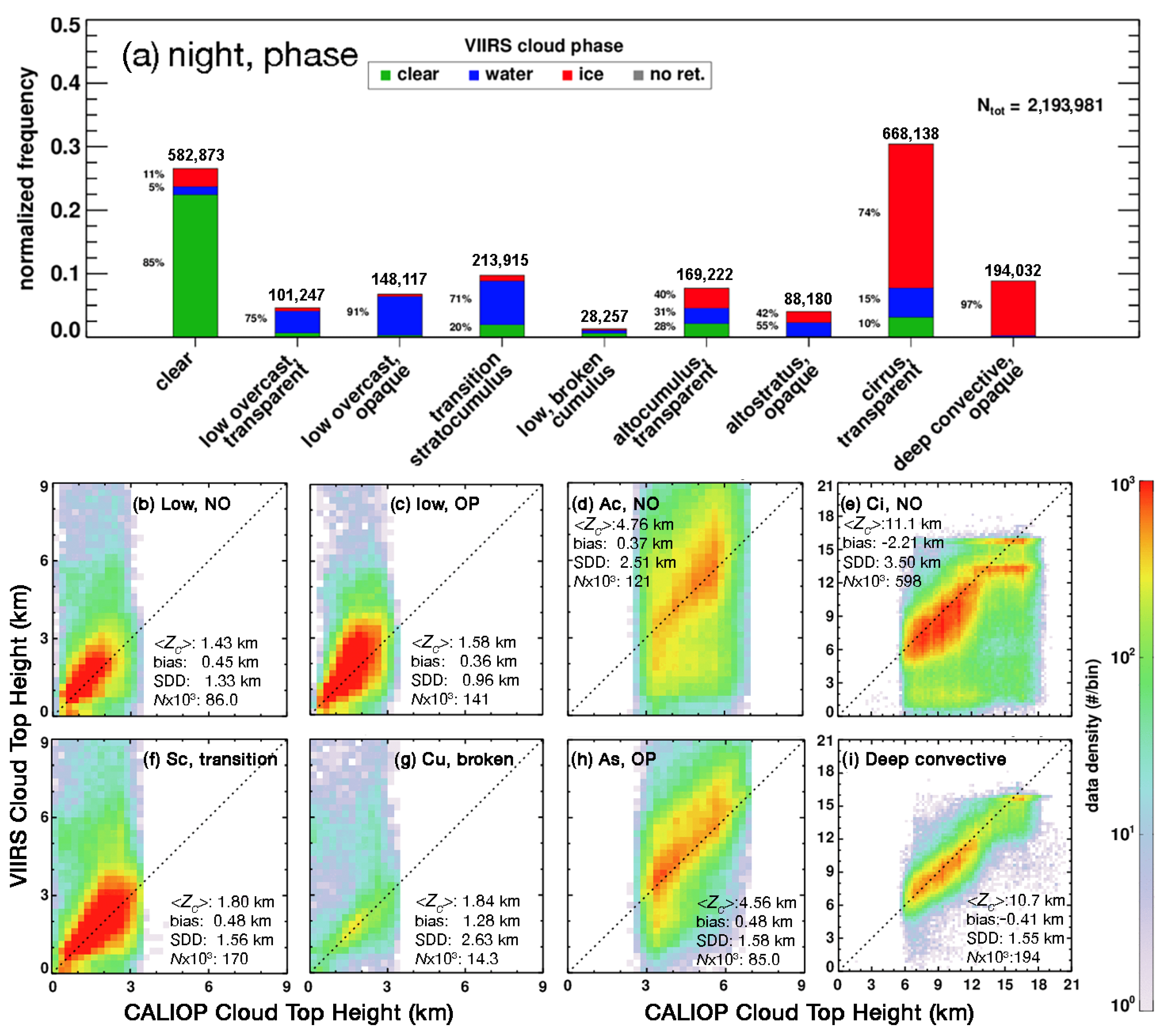
3.2. Cloud Phase
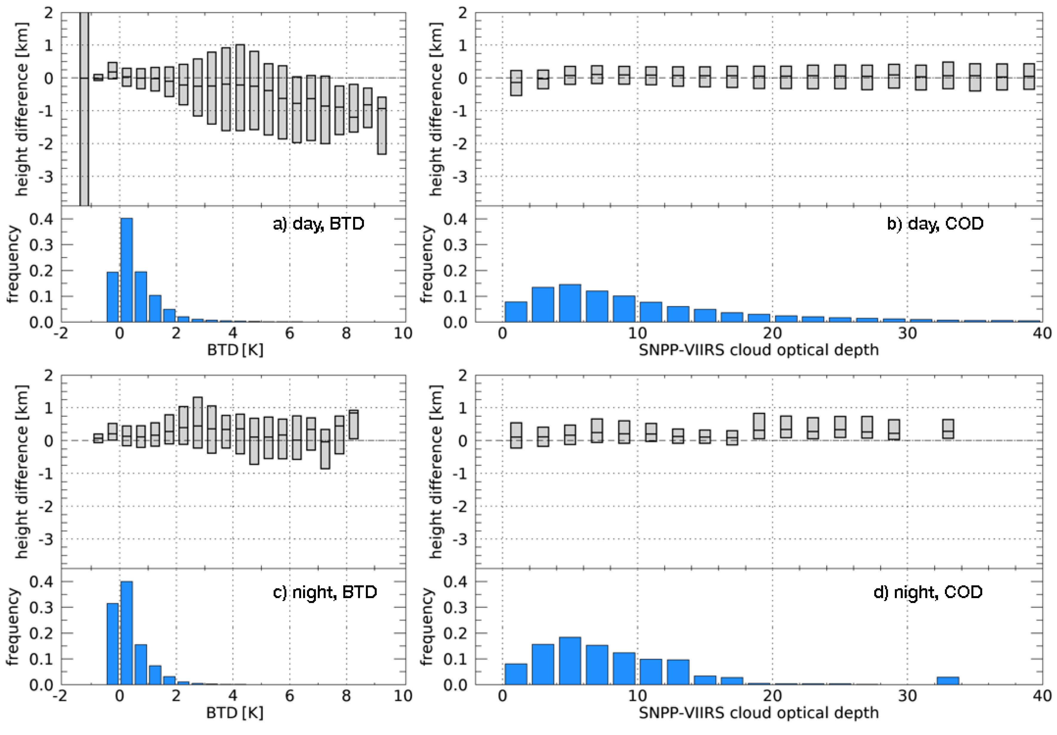
3.3. Cloud Top Height
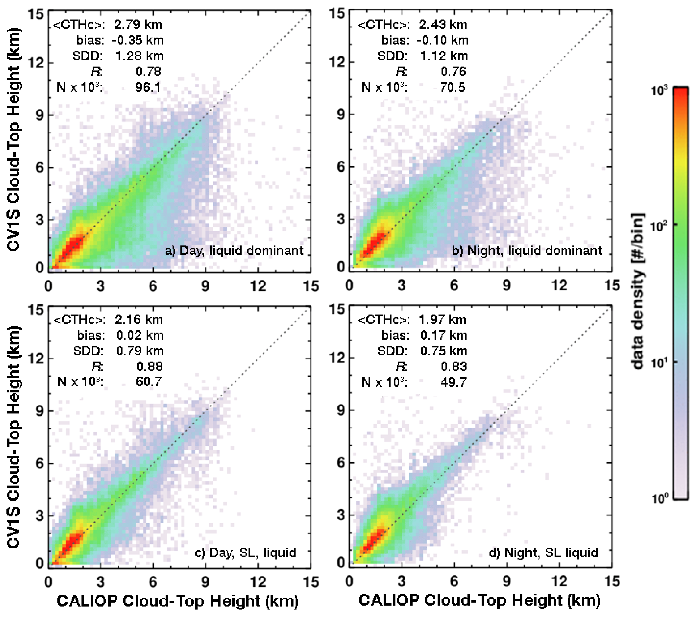
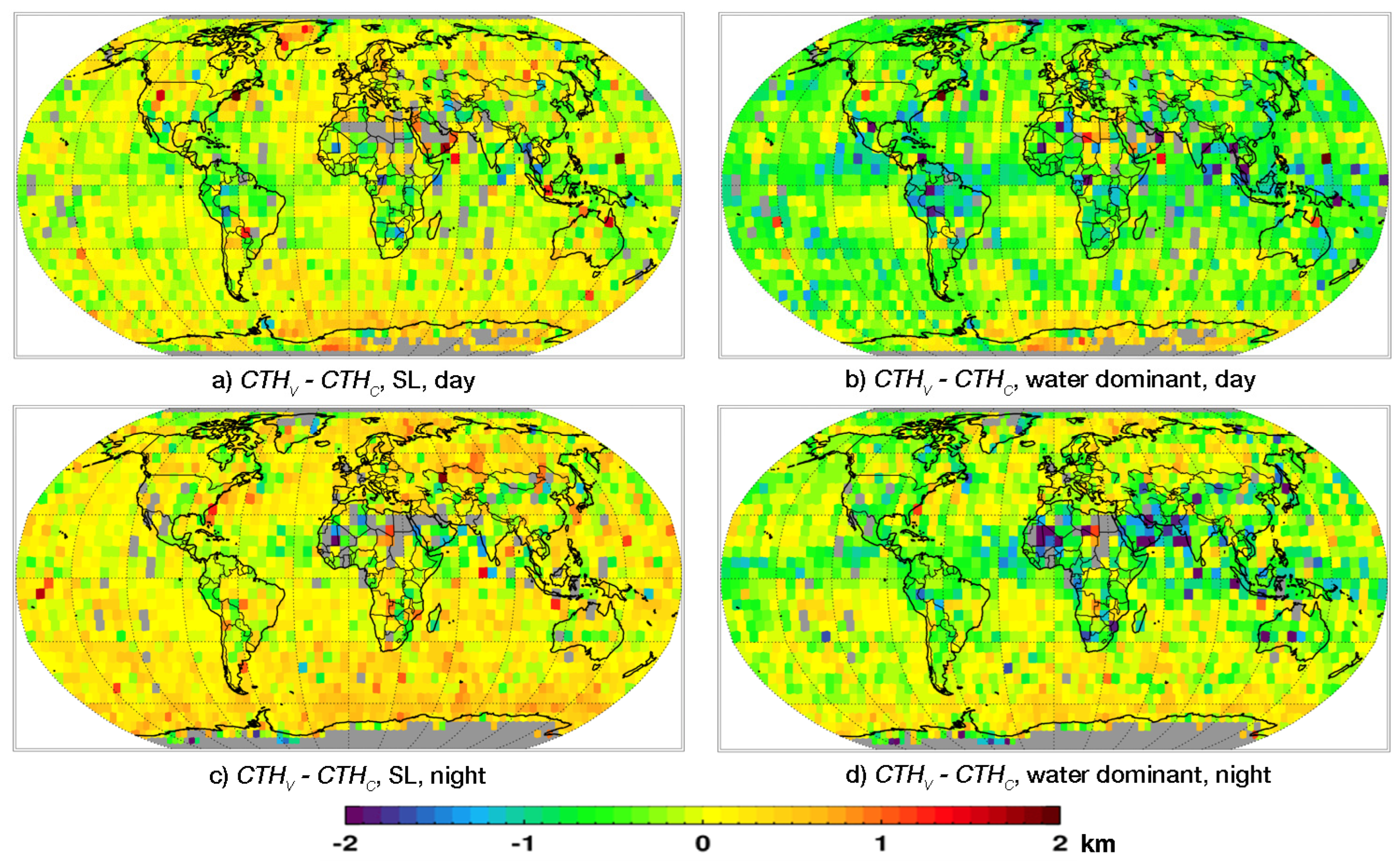
3.3.1. Liquid Clouds
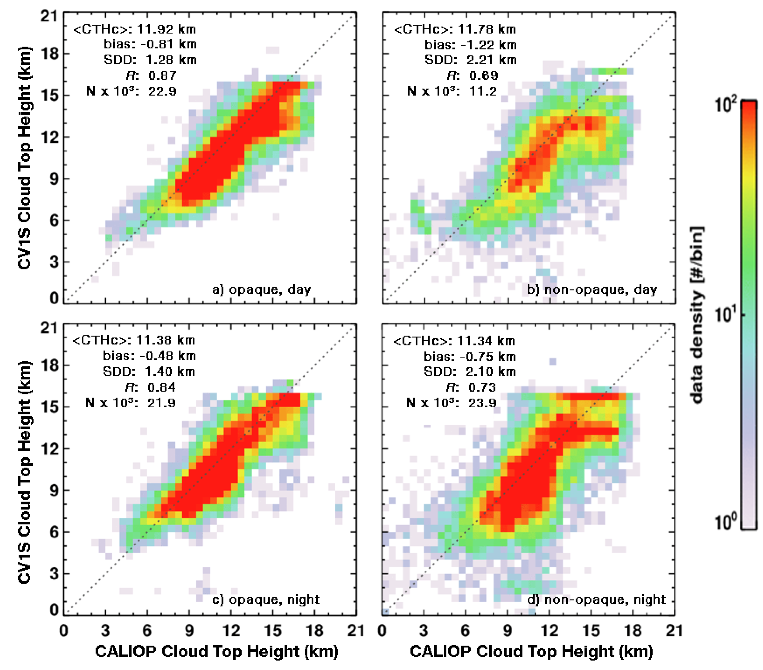
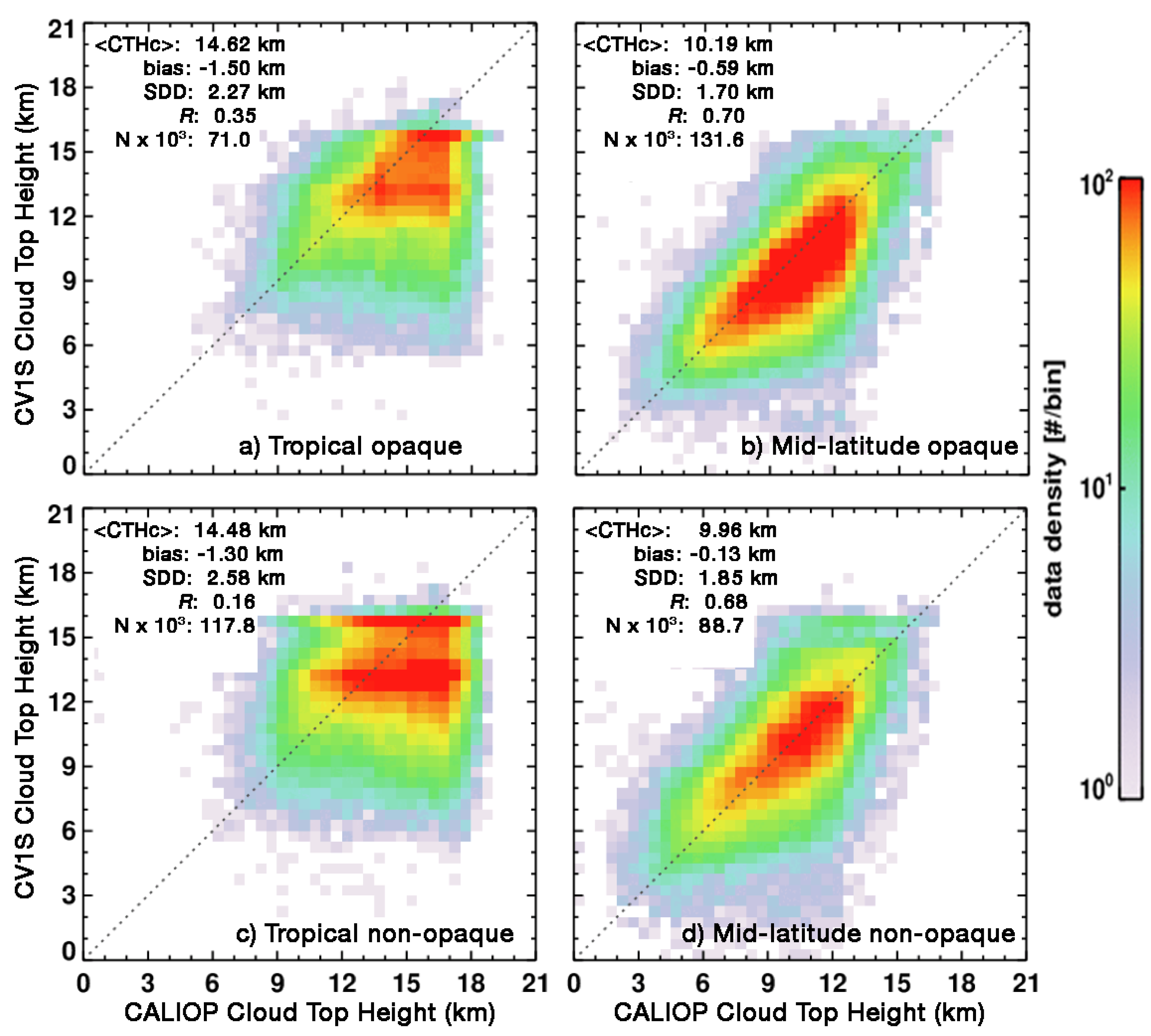
3.3.2. Ice Clouds
4. Discussion
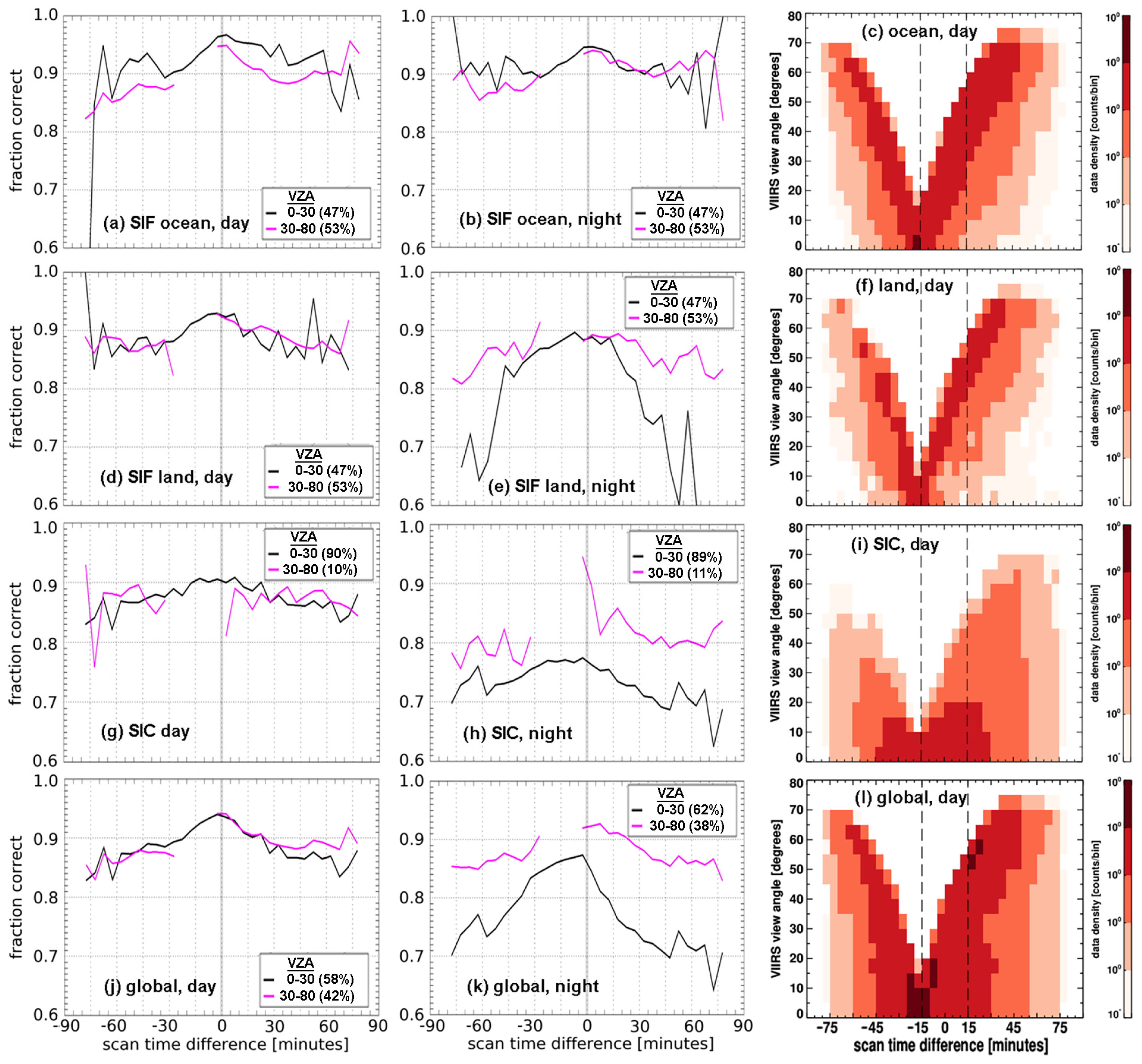
4.1. VZA and Time Window Dependence
4.2. Cloud Fraction: Comparison with Other Results
4.3. Cloud Phase
4.4. Cloud Top Heights
4.4.1. Liquid Water Cloud Heights
4.4.2. Ice Cloud Heights
4.4.3. All Cloud Heights
5. Conclusions
- -
- The accuracies of the CV1S cloud fraction are slightly better than those for CM4A during the daytime and about the same as those at night. CV1S cloud phase accuracy is slightly worse than CM4A during the day and night. Sensitivity of phase selection to ice cloud optical depth in multi-layered clouds is very consistent between CV1S and CM4A. The cloud-top height comparisons are very consistent with their CM4A counterparts with the exception of reduced ice cloud top height biases for CV1S, likely the result of using different channels for backup retrievals.
- -
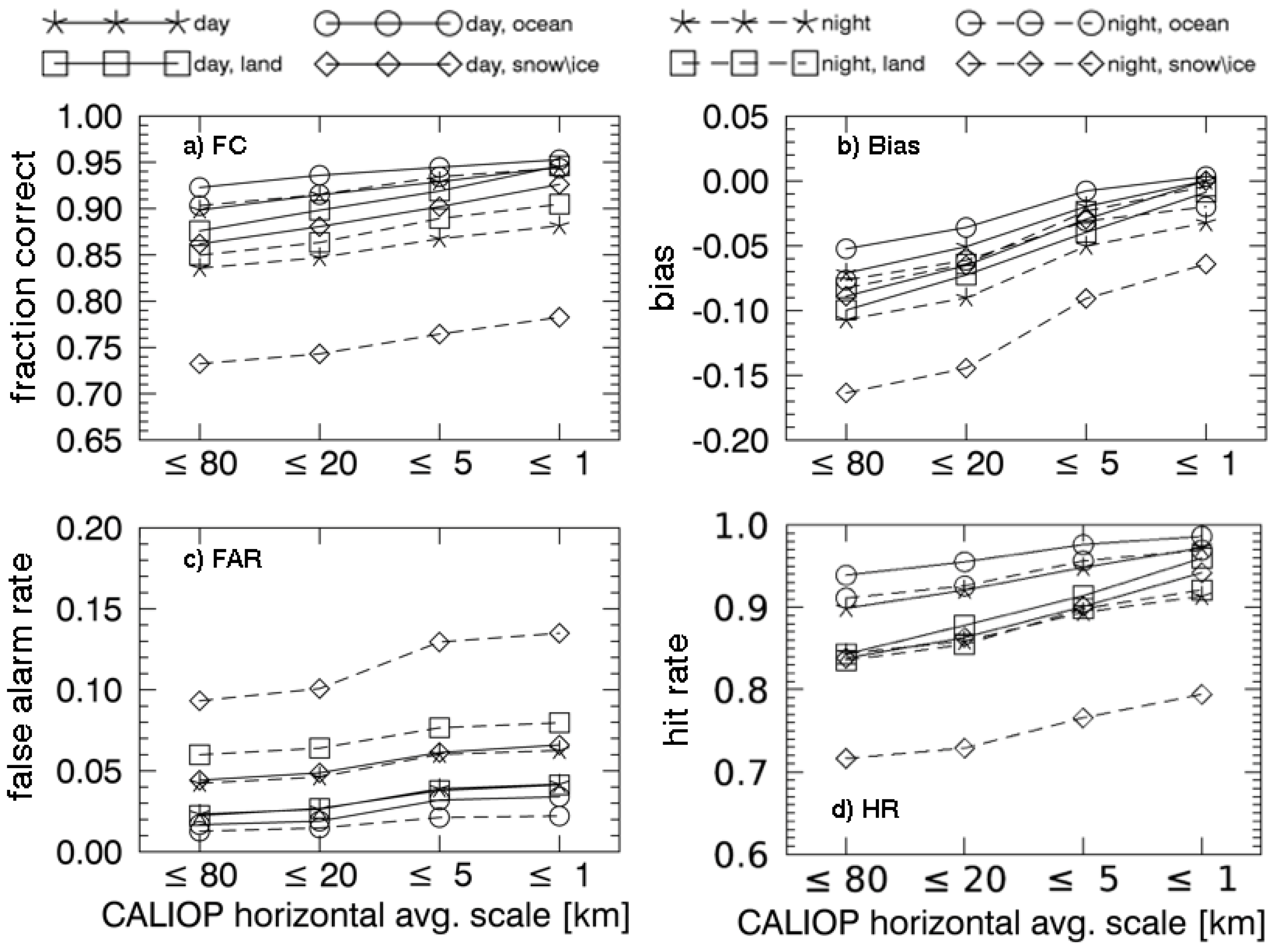
- The time window for matching CALIOP and imager data is very important for assessing instantaneous cloud amount, but is not as critical for determining cloud amount bias. Using a larger collocation time window than 5 min would have produced less consistency with CM4A for fraction correct. Imager VZA also has some impact on cloud fraction bias, particularly at night. VZA and time windows are less important for cloud phase and height assessment, except for thin cirrus at night. As seen in [19], the CALIOP detection resolution affects the bias.
- -
- Daytime CV1S cloud detection is as good or better than several other operational algorithms. At night, the accuracies are comparable overall with the other methods. None of the operational approaches are as accurate as a new machine learning technique for cloud detection.
- -
- Supercooled liquid water clouds are properly diagnosed 96% of the time during the daytime. At night, they are correctly identified in 75% of the cases. CV1S cloud phase accuracy overall is comparable to that from several operational methods but is slightly less than that from a new neural-net based method.
- -
- Liquid water cloud top heights are less biased during the daytime than at night. For single-layer clouds, the nocturnal bias is 0.2 km. Further research is need to assess that day–night difference. The transition of a surface-anchored lapse rate to a reanalysis temperature profile in assigning height to a given cloud temperature is responsible for underestimating cloud top height for many altostratus clouds.
- -
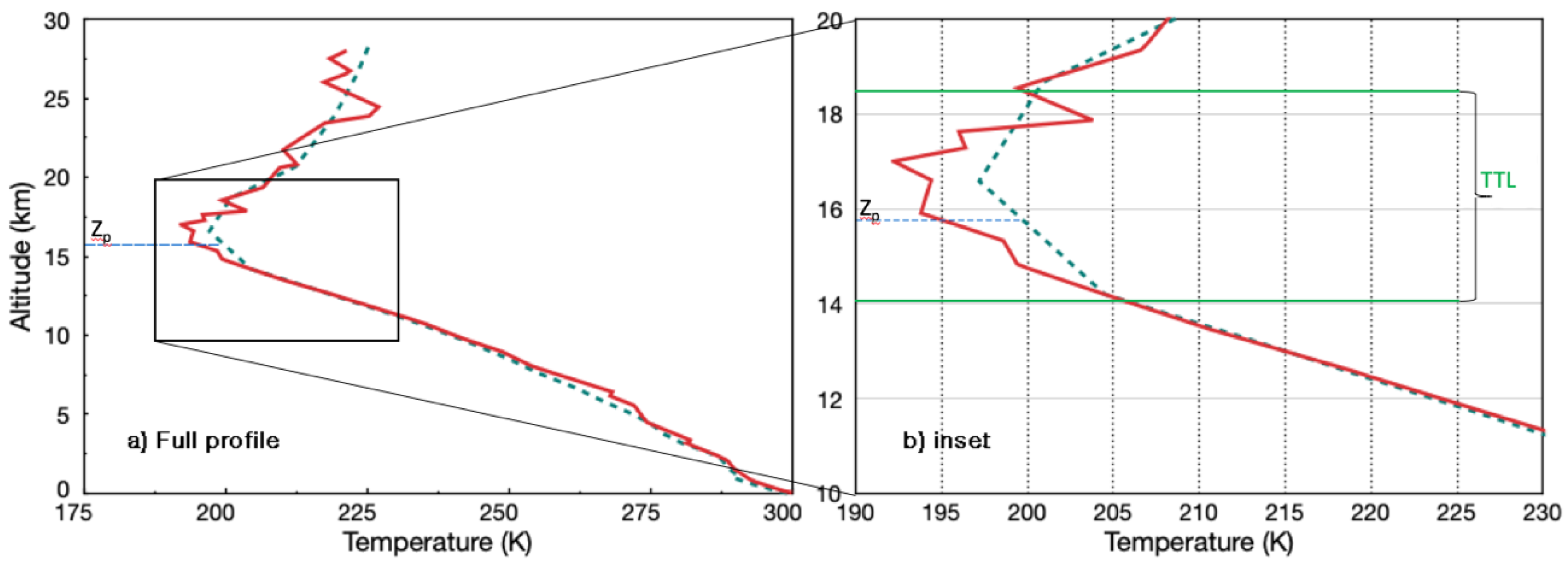
- Ice cloud top heights are underestimated in the tropics partially because CV1S confines the top to the tropopause level. That level is poorly determined in the tropics, and is set near the bottom of the tropical transition layer. Retrievals that initially might place the cloud higher are overwritten with the tropopause altitude, underestimating the top altitude of many clouds above 15 km. Other factors affecting the height retrieval, especially during daytime, are low-level clouds underneath both midlevel and high clouds.
- -
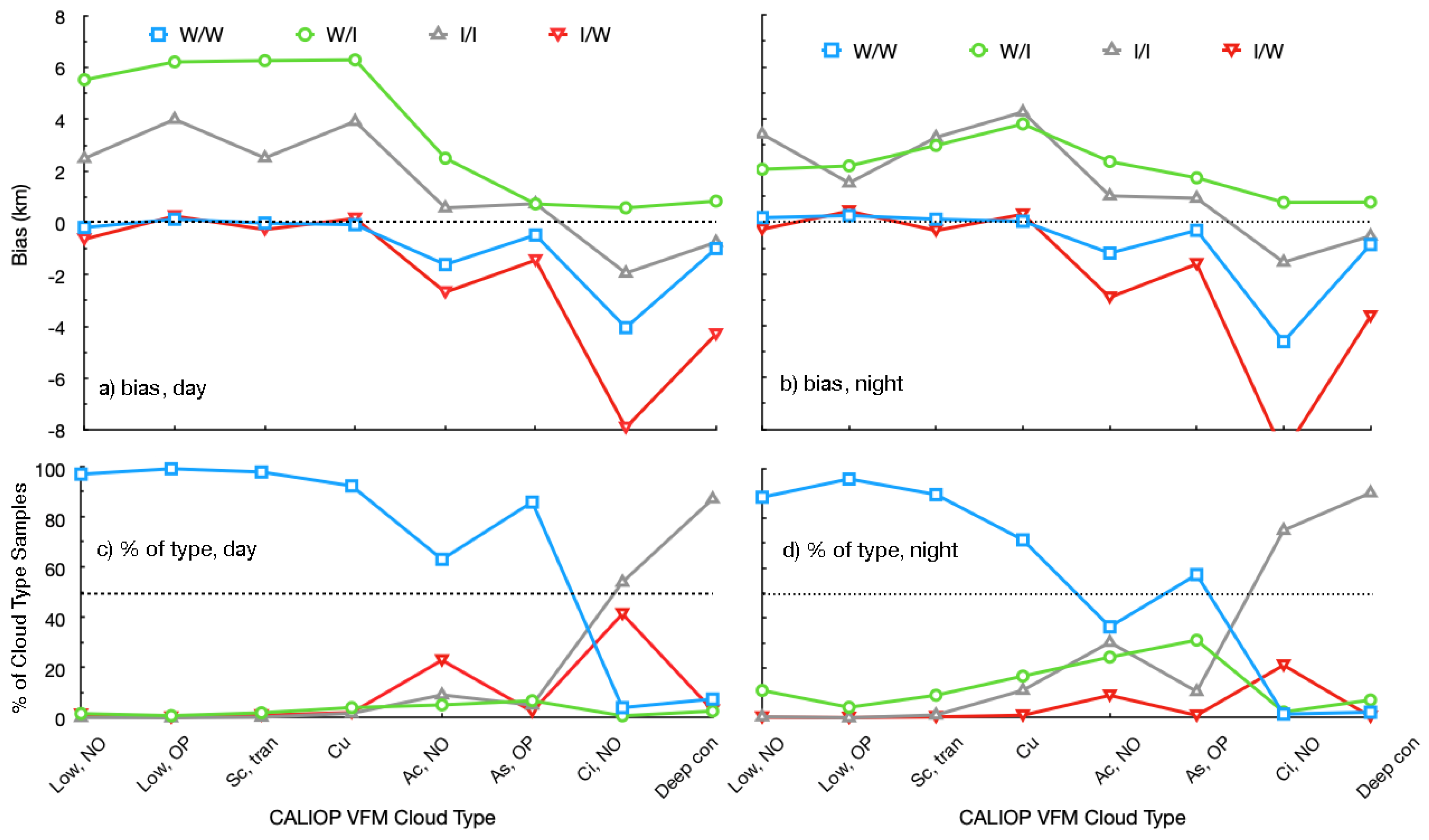
- Because cloud optical depth, effective temperature, effective hydrometeor radius, and phase are determined simultaneously, selecting the correct phase impacts the effective temperature. Inaccurate phase selection thus affects cloud-top height estimates, even in the absence of multilayered, multiphase clouds. Cloud altitude is overestimated significantly when liquid clouds are interpreted as ice clouds. The opposite effect is found for ice clouds classified as water. There is minimal dependence of this effect on the time of day.
- -
- CV1S cloud top height uncertainty overall is very similar to or better than several operational algorithms, but again, fails to match the accuracy of an experimental machine learning technique.
Author Contributions
Funding
Data Availability Statement
Acknowledgments
Conflicts of Interest
References
- Smith, G.L.; Priestley, K.J.; Loeb, N.G.; Wielicki, B.A.; Charlock, T.P.; Minnis, P.; Doelling, D.R.; Rutan, D.A. Clouds and the Earth’s Radiant Energy System (CERES), a review: Past, present, and future. Adv. Space Res. 2011, 48, 254–263. [Google Scholar] [CrossRef]
- Loeb, N.G.; Su, W.; Doelling, D.R.; Wong, T.; Minnis, P.; Thomas, S.; Miller, W.F. 5.03—Earth’s top-of-atmosphere radiation budget. In Comprehensive Remote Sensing; Elsevier Ltd.: Oxford, UK, 2018; pp. 67–84. [Google Scholar] [CrossRef]
- Hillger, D.; Kopp, T.; Lee, T.; Lindsey, D.; Seaman, C.; Miller, S.; Solberg, J.; Kidder, S.; Bachmeier, S.; Jasmin, T.; et al. First-light imagery from Suomi NPP VIIRS. Bull. Am. Meteorol. Soc. 2013, 93, 1019–1029. [Google Scholar] [CrossRef]
- Minnis, P.; Sun-Mack, S.; Smith, W.L., Jr.; Trepte, Q.Z.; Hong, G.; Chen, Y.; Yost, C.R.; Chang, F.-L.; Smith, R.A.; Heck, P.W.; et al. VIIRS Edition 1 cloud properties for CERES. Part 1: Algorithm adjustments and results. Remote Sens. 2023, 15, 578. [Google Scholar] [CrossRef]
- Winker, D.M.; Vaughan, M.A.; Omar, A.; Hu, Y.; Powell, K.A.; Liu, Z.; Hunt, W.H.; Young, S.A. Overview of the CALIPSO mission and CALIOP data processing algorithms. J. Atmos. Ocean. Technol. 2009, 26, 2310–2323. [Google Scholar] [CrossRef]
- Sun-Mack, S.; Wielicki, B.A.; Minnis, P.; Gibson, S.; Chen, Y. Integrated cloud-aerosol-radiation product using CERES, MODIS, CALIPSO, and CloudSat data. Proc. SPIE Remote Sens. Clouds Atmos. XII 2007, 6745, 674513. [Google Scholar] [CrossRef]
- Minnis, P.; Yost, C.R.; Sun-Mack, S.; Chen, Y. Estimating the physical top altitude of optically thick ice clouds from thermal infrared satellite observations using CALIPSO data. Geophys. Res. Lett. 2008, 35, L12801. [Google Scholar] [CrossRef]
- Holz, R.E.; Ackerman, S.A.; Nagle, F.W.; Frey, R.; Dutcher, S.; Kuehn, R.E.; Vaughan, M.A.; Baum, B. Global moderate resolution imaging spectroradiometer (MODIS) cloud detection and height evaluation using CALIOP. J. Geophys. Res. 2008, 113, D00A19. [Google Scholar] [CrossRef]
- Karlsson, K.-G.; Johansson, E. On the optimal method for evaluating cloud products from passive satellite imagery using CALIPSO-CALIOP data: Example investigating the CM SAF CLARA-A1 dataset. Atmos. Meas. Tech. 2013, 6, 1271–1286. [Google Scholar] [CrossRef]
- Kox, S.; Bugliaro, L.; Ostler, A. Retrieval of cirrus cloud optical thickness and top altitude from geostationary remote sensing. Atmos. Meas. Tech. 2014, 7, 3233–3246. [Google Scholar] [CrossRef]
- Marchant, B.; Platnick, S.; Meyer, K.; Arnold, G.T.; Riedi, J. MODIS Collection 6 shortwave-derived cloud phase classification algorithm and comparisons with CALIOP. Atmos. Meas. Tech. 2016, 9, 1587–1599. [Google Scholar] [CrossRef]
- Håkansson, N.; Adok, C.; Thoss, A.; Scheirer, R.; Hörnquist, S. Neural network cloud top pressure and height for MODIS. Atmos. Meas. Tech. 2018, 11, 3177–3196. [Google Scholar] [CrossRef]
- Karlsson, K.-G.; Håkansson, N. Characterization of AVHRR global cloud detection sensitivity based on CALIPSO-CALIOP cloud optical thickness information: Demonstration of results based on the CM SAF CLARA-A2 climate data record. Atmos. Meas. Tech. 2018, 11, 633–649. [Google Scholar] [CrossRef]
- Wang, C.; Platnick, S.; Fauchez, T.; Meyer, K.; Zhang, Z.; Iwabuchi, H.; Kahn, B.H. An assessment of the impacts of cloud vertical heterogeneity on global ice cloud data records from passive satellite retrievals. J. Geophys. Res. 2019, 124, 1578–1595. [Google Scholar] [CrossRef]
- Marchant, B.; Platnick, S.; Meyer, K.; Wind, G. Evaluation of the Aqua MODIS Collection 6.1 multilayer cloud detection algorithm through comparisons with CloudSat CPR and CALIPSO CALIOP products. Atmos. Meas. Tech. 2020, 13, 3263–3275. [Google Scholar] [CrossRef]
- Frey, R.A.; Ackerman, S.A.; Holz, R.E.; Dutcher, S.; Griffith, Z. The continuity MODIS-VIIRS cloud mask. Remote Sens. 2020, 12, 3334. [Google Scholar] [CrossRef]
- Jiménez, P.A. Assessment of the GOES-16 clear sky mask product over the contiguous USA using CALIPSO retrievals. Remote Sens. 2020, 12, 1630. [Google Scholar] [CrossRef]
- Li, Y.; Baum, B.A.; Heidinger, A.K.; Menzel, W.P.; Weise, E. Improvement in cloud retrievals from VIIRS through use of infrared absorption channels constructed from VIIRS+CrIS data fusion. Atmos. Meas. Tech. 2020, 13, 4035–4049. [Google Scholar] [CrossRef]
- Yost, C.; Minnis, P.; Sun-Mack, S.; Chen, Y.; Smith, W.L., Jr. CERES MODIS cloud product retrievals for Edition 4, Part II: Comparisons to CloudSat and CALIPSO. IEEE Trans. Geosci. Remote Sens. 2021, 59, 3695–3724. [Google Scholar] [CrossRef]
- Trepte, Q.Z.; Minnis, P.; Sun-Mack, S.; Yost, C.R.; Chen, C.R.; Jin, Z.; Chang, F.-L.; Smith, W.L., Jr.; Bedka, K.M.; Chee, T.L. Global cloud detection for CERES Edition 4 using Terra and Aqua MODIS data. IEEE Trans. Geosci. Remote Sens. 2019, 57, 9410–9449. [Google Scholar] [CrossRef]
- Stephens, G.L.; Vane, D.G.; Tanelli, S.; Im, E.; Durden, S.; Rokey, M.; Reinke, D.; Partain, P.; Mace, G.G.; Austin, R.; et al. CloudSat mission: Performance and early science after the first year of operation. J. Geophys. Res. 2008, 113, D00A18. [Google Scholar] [CrossRef]
- Vaughan, M.A.; Powell, K.A.; Kuehn, R.E.; Young, S.A.; Winker, D.M.; Hostetler, C.A.; Hunt, W.H.; Liu, Z.; McGill, M.J.; Getzewitch, B.J. Fully automated detection of cloud and aerosol layers in the CALIPSO lidar measurements. J. Atmos. Ocean. Technol. 2009, 26, 2034–2050. [Google Scholar] [CrossRef]
- Vaughan, M.A.; Pitts, M.; Trepte, C.; Winker, D.; Detweiler, P.; Garnier, A.; Getzewich, B.; Hunt, W.; Lambeth, J.; Lee, K.-P.; et al. Cloud-Aerosol LIDAR Infrared Pathfinder Satellite Observations (CALIPSO) Data Management System Data Products Catalog, Release 4.10; NASA Langley Research Center Document PC-SCI-503; NASA Langley Research Center: Hampton, VA, USA, 2016. [Google Scholar]
- Hu, Y.; Winker, D.; Vaughan, M.; Lin, B.; Omar, A.; Trepte, C.; Flittner, D.; Yang, P.; Baum, B.; Sun, W.; et al. CALIPSO/CALIOP cloud phase discrimination algorithm. J. Atmos. Ocean. Technol 2009, 26, 2293–2309. [Google Scholar] [CrossRef]
- Young, S.A.; Vaughan, M.A.; Tackett, J.L.; Garnier, A.; Lambeth, J.B.; Powell, K.A. Extinction and optical depth retrievals for CALIPSO’s Version 4 data release. Atmos. Meas. Tech. 2018, 11, 5701–5727. [Google Scholar] [CrossRef]
- White, C.H.; Heidinger, A.K.; Ackerman, S.A. Evaluation of Visible Infrared Imaging Radiometer Suite (VIIRS) neural network cloud detection against current operational cloud masks. Atmos. Meas. Tech. 2021, 14, 3371–3394. [Google Scholar] [CrossRef]
- Woodcock, F. The evaluation of yes/no forecasts for scientific and administrative purposes. Mon. Weather Rev. 1976, 104, 1209–1214. [Google Scholar] [CrossRef]
- Heidinger, A.; Botambekov, D.; Walther, A. A Naïve Bayesian Cloud Mask Delivered to NOAA Enterprise—Version 1.2; Tech. Rep.; NOAA NESDIS Center for Satellite Applications and Research: Silver Spring, MD, USA, 2016. Available online: https://www.star.nesdis.noaa.gov/goesr/documents/ATBDs/Enterprise/ATBD_Enterprise_Cloud_Mask_v1.2_Oct2016.pdf (accessed on 21 July 2020).
- Wang, C.; Platnick, S.; Meyer, K.; Zhang, Z.; Zhou, Y. A machine-learning-based cloud detection and thermodynamic-phase classification algorithm using passive spectral observations. Atmos. Meas. Tech. 2020, 13, 2257–2277. [Google Scholar] [CrossRef]
- Zhou, G.; Wang, J.; Yin, Y.; Hu, X.; Letu, H.; Sohn, B.-J.; Chao, L. Detecting supercooled water clouds using passive radiometer measurements. Geophys. Res. Lett. 2022, 49, e2021GL096111. [Google Scholar] [CrossRef]
- Sassen, K.; Wang, Z.; Liu, D. Global distribution of cirrus clouds from CloudSat/Cloud-Aerosol Lidar and Infrared Pathfinder Satellite Observations (CALIPSO) measurements. J. Geophys. Res. 2008, 113, D00A12. [Google Scholar] [CrossRef]
- Platnick, S.; Meyer, K.; Wind, G.; Holz, R.E.; Amarasinghe, N.; Hubanks, P.A.; Marchant, B.; Dutcher, S.; Veglio, P. The NASA MODIS-VIIRS continuity cloud optical properties products. Remote Sens. 2021, 13, 2. [Google Scholar] [CrossRef]
- Minnis, P.; Sun-Mack, S.; Young, D.F.; Heck, P.W.; Garber, D.P.; Chen, Y.; Spangenberg, D.A.; Arduini, R.F.; Trepte, Q.Z.; Smith, W.L., Jr.; et al. CERES Edition-2 cloud property retrievals using TRMM VIRS and Terra and Aqua MODIS data, Part I: Algorithms. IEEE Trans. Geosci. Remote Sens. 2011, 49, 4374–4400. [Google Scholar] [CrossRef]
- Sun-Mack, S.; Minnis, P.; Chen, Y.; Kato, S.; Yi, Y.; Gibson, S.; Heck, P.W.; Winker, D. Regional apparent boundary layer lapse rates determined from CALIPSO and MODIS data for cloud height determination. J. Appl. Meteorol. Climatol. 2014, 53, 990–1011. [Google Scholar] [CrossRef]
- Rienecker, M.M.; Suarez, M.J.; Todling, R.; Bacmeister, S.; Takacs, L.; Liu, H.-C.; Gu, W.; Sienkiewicz, M.; Koster, R.D.; Gelaro, R.; et al. The GEOS-5 Data Assimilation System—Documentation of Versions 5.0.1, 5.1.0, and 5.2.0; Technical Report Series on Global Modeling and Data Assimilation, Report No. NASA/TM-2008-104606-VOL-27; NASA: Washington, DC, USA, 2008; Volume 27, 118p. [Google Scholar]
- Minnis, P.; Sun-Mack, S.; Yost, C.R.; Chen, Y.; Smith, W.L., Jr.; Chang, F.-L.; Heck, P.W.; Arduini, R.F.; Trepte, Q.Z.; Ayers, K.; et al. CERES MODIS cloud product retrievals for Edition 4, Part I: Algorithm changes to CERES MODIS. IEEE Trans. Geosci. Remote Sens. 2021, 59, 2744–2780. [Google Scholar] [CrossRef]
- Baum, B.A.; Arduini, R.F.; Wielicki, B.A.; Minnis, P.; Tsay, S.-C. Multilevel cloud retrieval using multispectral HIRS and AVHRR data: Nighttime oceanic analysis. J. Geophys. Res. 1994, 99, 5499–5514. [Google Scholar] [CrossRef]
- Zheng, Y.; Li, Z. Episodes of warm air advection causing cloud-surface decoupling during MARCUS. J. Geophys. Res. Atmos. 2019, 124, 12227–12443. [Google Scholar] [CrossRef]
- Minnis, P.; Sun-Mack, S.; Chen, Y.; Khaiyer, M.M.; Yi, Y.; Ayers, J.K.; Brown, R.R.; Dong, X.; Gibson, S.C.; Heck, P.W.; et al. CERES Edition-2 cloud property retrievals using TRMM VIRS and Terra and Aqua MODIS data, Part II: Examples of average results and comparisons with other data. IEEE Trans. Geosci. Remote Sens. 2011, 49, 4401–4430. [Google Scholar] [CrossRef]
- Fueglistaler, S.; Dessler, A.E.; Dunkerton, T.J.; Folkins, I.; Fu, Q.; Mote, P.W. Tropical tropopause layer. Rev. Geophys. 2009, 47, RG1004. [Google Scholar] [CrossRef]
- Loeb, N.; Yang, P.; Rose, F.G.; Hong, G.; Sun-Mack, S.; Minnis, P.; Kato, S.; Ham, S.-H.; Smith, W.L., Jr. Impact of ice cloud microphysics on satellite retrievals and broadband flux radiative transfer calculations. J. Clim. 2018, 31, 1851–1864. [Google Scholar] [CrossRef]
- Baum, B.A.; Menzel, W.P.; Frey, R.A.; Tobin, D.C.; Holz, R.E.; Ackerman, S.A.; Heidinger, A.K.; Yang, P. MODIS cloud-top property refinements for Collection 6. J. Appl. Meteorol. Climatol. 2012, 51, 1145–1163. [Google Scholar] [CrossRef]
- Stengel, M.; Stapelberg, S.; Sus, O.; Schlundt, C.; Poulsen, C.; Thomas, G.; Christensen, M.; Carbajal Henken, C.; Preusker, R.; Fischer, J.; et al. Cloud property datasets retrieved from AVHRR, MODIS, AATSR and MERIS in the framework of the Cloud_cci project. Earth Syst. Sci. Data 2017, 9, 881–904. [Google Scholar] [CrossRef]
- Minnis, P.; Young, D.F.; Sassen, K.; Alvarez, J.M.; Grund, C.J. The 27-28 October 1986 FIRE IFO Case Study: Cirrus parameter relationships derived from satellite and lidar data. Mon. Weather Rev. 1990, 118, 2402–2425. [Google Scholar] [CrossRef]
- Sherwood, S.C.; Chae, J.-H.; Minnis, P.; McGill, M. Underestimation of deep convective cloud tops by thermal imagery. Geophys. Res. Lett. 2004, 31, L11102. [Google Scholar] [CrossRef]
- Nakajima, T.Y.; Ishida, H.; Nagao, T.M.; Hori, M.; Letu, H.; Higuchi, R.; Tamaru, N.; Imoto, N.; Yamazaki, A. Theoretical basis of the algorithms and early phase results of the GCOM-C (Shikisai) SGLI cloud products. Prog. Earth Planet. Sci. 2019, 6, 52. [Google Scholar] [CrossRef]
- Minnis, P.; Sun-Mack, S.; Smith, W.L., Jr.; Hong, G.; Chen, Y. Advances in neural network detection and retrieval of multilayer clouds for CERES using multispectral satellite data. Proc. SPIE Remote Sens. Clouds and the Atmos. XXIV 2019, 11152, 1115202. [Google Scholar] [CrossRef]


| VIIRS | CALIPSO | ||
|---|---|---|---|
| Clear (Liquid) | Cloudy (Ice) | Sum | |
| Clear (liquid) | Tn | Fn | n |
| Cloudy (ice) | Fp | Tp | p |
| Day | FC | HR | Bias | FAR | HKSS | N × 103 |
| Nonpolar | 0.952 (0.896) | 0.959 (0.914) | −0.011 (−0.012) | 0.026 (0.069) | 0.885 (0.765) | 220 (272) |
| Polar | 0.923 (0.899) | 0.923 (0.902) | −0.024 (−0.029) | 0.041 (0.057) | 0.831 (0.779) | 99 (108) |
| Global, All | 0.943 (0.897) | 0.948 (0.910) | −0.015 (−0.017) | 0.030 (0.066) | 0.868 (0.769) | 318 (380) |
| Global, All * | 0.948 (0.896) | 0.954 (0.912) | −0.013 (−0.014) | 0.028 (0.067) | 0.878 (0.767) | - |
| Night | ||||||
| Nonpolar | 0.927 (0.870) | 0.941 (0.890) | −0.018 (−0.035) | 0.037 (0.070) | 0.798 (0.697) | 213 (271) |
| Polar | 0.804 (0.764) | 0.809 (0.777) | −0.080 (−0.068) | 0.091 (0.127) | 0.551 (0.476) | 126 (151) |
| Global, All | 0.881 (0.833) | 0.913 (0.846) | −0.041 (−0.050) | 0.055 (0.090) | 0.698 (0.616) | 339 (422) |
| Global, All * | 0.911 (0.856) | 0.924 (0.875) | −0.026 (−0.039) | 0.044 (0.077) | 0.765 (0.669) | - |
| Day | Fraction Correct | Bias | Ice FAR | Water FAR | HKSS | Number Samples (×103) |
| Global, All surfaces | 0.931 | −0.019 | 0.068 | 0.069 | 0.844 | 132 |
| Nonpolar land, SIF | 0.888 | −0.079 | 0.034 | 0.182 | 0.791 | 19 |
| Polar land, SIF | 0.920 | −0.038 | 0.073 | 0.082 | 0.789 | 4 |
| Nonpolar ocean, SIF | 0.954 | −0.005 | 0.055 | 0.040 | 0.900 | 75 |
| Polar ocean, SIF | 0.941 | +0.005 | 0.160 | 0.034 | 0.820 | 10 |
| Global, SIF | 0.940 | −0.018 | 0.056 | 0.062 | 0.866 | 108 |
| Global, SIC | 0.892 | −0.023 | 0.131 | 0.097 | 0.746 | 25 |
| Nighttime | ||||||
| Global, All surfaces | 0.883 | 0.079 | 0.185 | 0.040 | 0.780 | 141 |
| Nonpolar land, SIF | 0.854 | 0.025 | 0.140 | 0.155 | 0.690 | 18 |
| Polar land, SIF | 0.869 | 0.099 | 0.219 | 0.033 | 0.762 | 3 |
| Nonpolar ocean, SIF | 0.909 | 0.060 | 0.186 | 0.026 | 0.840 | 72 |
| Polar ocean, SIF | 0.883 | 0.098 | 0.278 | 0.015 | 0.816 | 10 |
| Global, SIF | 0.896 | 0.059 | 0.185 | 0.040 | 0.809 | 103 |
| Global, SIC | 0.849 | 0.135 | 0.186 | 0.035 | 0.596 | 38 |
| Single Layer Only | All with Liquid Top | |||||
|---|---|---|---|---|---|---|
| Day | Bias (SDD) [km] | R | Number of Matches × 103 | Bias (SDD) [km] | R | Number of Matches × 103 |
| Land, SIF | 0.05 (0.98) | 0.86 | 6.5 | −0.41 (1.37) | 0.77 | 14.2 |
| Ocean, SIF | 0.00 (0.74) | 0.88 | 42.7 | −0.38 (1.27) | 0.77 | 62.4 |
| SIC | 0.09 (0.87) | 0.85 | 11.5 | −0.24 (1.24) | 0.70 | 19.5 |
| Global, All | 0.02 (0.79) | 0.88 | 60.7 | −0.35 (1.28) | 0.78 | 96.1 |
| Night | ||||||
| Land, SIF | 0.18 (0.94) | 0.86 | 4.9 | −0.17 (1.27) | 0.79 | 8.0 |
| Ocean, SIF | 0.16 (0.71) | 0.80 | 38.5 | −0.10 (1.11) | 0.73 | 53.2 |
| SIC | 0.21 (0.81) | 0.76 | 6.3 | 0.00 (1.02) | 0.68 | 9.3 |
| Global, All | 0.17 (0.75) | 0.83 | 49.7 | −0.10 (1.12) | 0.76 | 70.5 |
| Single Layer Ice Only | All with Ice Top | |||||
|---|---|---|---|---|---|---|
| Day | Bias (SDD) [km] | R | Number of Matches × 10−3 | Bias (SDD) [km] | R | Number of Matches × 10−3 |
| Land, SIF | −0.56 (1.96) | 0.59 | 2.6 | −0.85 (2.14) | 0.67 | 4.5 |
| Ocean, SIF | −1.44 (2.21) | 0.53 | 6.0 | −1.54 (2.28) | 0.62 | 11.1 |
| SIC | −1.35 (2.30) | 0.46 | 2.6 | −1.30 (2.14) | 0.51 | 5.6 |
| Global, All | −1.22 (2.21) | 0.69 | 11.2 | −1.33 (2.23) | 0.74 | 21.3 |
| Night | ||||||
| Land, SIF | −0.27 (2.01) | 0.65 | 4.8 | −0.55 (2.25) | 0.71 | 9.1 |
| Ocean, SIF | −0.26 (1.84) | 0.68 | 8.8 | −0.69 (2.28) | 0.71 | 25.0 |
| SIC | −1.40 (2.17) | 0.64 | 10.3 | −0.97 (2.43) | 0.44 | 22.4 |
| Global, All | −0.75 (2.10) | 0.73 | 23.9 | −0.78 (2.34) | 0.74 | 56.5 |
| Single Layer Ice Only | All with Ice Top | |||||
|---|---|---|---|---|---|---|
| Day | Bias (SDD) [km] | R | Number of Matches × 10−3 | Bias (SDD) [km] | R | Number of Matches × 10−3 |
| Land, SIF | −0.47 (1.25) | 0.86 | 5.2 | −0.89 (1.53) | 0.84 | 8.8 |
| Ocean, SIF | −0.93 (1.27) | 0.86 | 16.1 | −1.35 (1.61) | 0.83 | 29.7 |
| SIC | −0.74 (1.29) | 0.71 | 1.6 | −1.13 (1.61) | 0.63 | 4.2 |
| Global, All | −0.81 (1.28) | 0.87 | 22.9 | −1.24 (1.60) | 0.84 | 42.7 |
| Night | ||||||
| Land, SIF | −0.38 (1.42) | 0.84 | 3.8 | −1.01 (2.01) | 0.75 | 7.5 |
| Ocean, SIF | −0.37 (1.27) | 0.86 | 12.8 | −0.83 (1.77) | 0.78 | 27.4 |
| SIC | −0.83 (1.61) | 0.62 | 5.4 | −0.96 (1.89) | 0.59 | 11.8 |
| Global, All | −0.48 (1.40) | 0.84 | 21.9 | −0.89 (1.84) | 0.78 | 46.7 |
| 0/100 | Day | Night | ||||||
| BACC | TPR | TNR | N × 103 | BACC | TPR | TNR | N × 103 | |
| Global | 0.953 | 0.970 | 0.937 | 297 | 0.878 | 0.902 | 0.853 | 343 |
| Water | 0.958 | 0.981 | 0.935 | 187 | 0.916 | 0.939 | 0.892 | 206 |
| Land | 0.940 | 0.941 | 0.939 | 110 | 0.825 | 0.819 | 0.831 | 137 |
| Sea Ice | 0.959 | 0.954 | 0.964 | 27 | 0.823 | 0.838 | 0.809 | 43 |
| Perm. snow | 0.908 | 0.908 | 0.908 | 32 | 0.760 | 0.703 | 0.817 | 58 |
| Snow land | 0.911 | 0.913 | 0.909 | 44 | 0.774 | 0.740 | 0.808 | 79 |
| 50/50 | Day | Night | ||||||
| Global | 0.887 | 0.919 | 0.855 | 396 | 0.824 | 0.850 | 0.798 | 470 |
| Water | 0.885 | 0.935 | 0.834 | 250 | 0.854 | 0.883 | 0.826 | 292 |
| Land | 0.878 | 0.881 | 0.876 | 145 | 0.775 | 0.776 | 0.774 | 178 |
| Sea Ice | 0.924 | 0.926 | 0.920 | 33 | 0.769 | 0.807 | 0.731 | 57 |
| Perm. snow | 0.869 | 0.871 | 0.867 | 39 | 0.713 | 0.663 | 0.763 | 74 |
| Snow land | 0.865 | 0.873 | 0.857 | 55 | 0.724 | 0.698 | 0.749 | 102 |
| All (km) | Low (km) | Midlevel (km) | High (km) | |||||
|---|---|---|---|---|---|---|---|---|
| Method | ∆ZT | MAE | ∆ZT | MAE | ∆ZT | MAE | ∆ZT | MAE |
| PPS | −1.47 | 2.09 | 0.31 | 0.85 | −0.35 | 1.12 | −3.46 | 3.56 |
| MOD C6 | −1.15 | 1.92 | 0.22 | 0.95 | −0.71 | 1.76 | −2.54 | 2.85 |
| HNN | −0.41 | 1.19 | 0.39 | 0.53 | 0.22 | 0.83 | −1.36 | 1.90 |
| CV1S100 | −0.99 | 1.92 | 0.38 | 0.80 | −0.10 | 1.58 | −2.17 | 2.75 |
| CV1S50 | −0.97 | 1.95 | 0.43 | 0.86 | −0.09 | 1.62 | −2.23 | 2.82 |
Disclaimer/Publisher’s Note: The statements, opinions and data contained in all publications are solely those of the individual author(s) and contributor(s) and not of MDPI and/or the editor(s). MDPI and/or the editor(s) disclaim responsibility for any injury to people or property resulting from any ideas, methods, instructions or products referred to in the content. |
© 2023 by the authors. Licensee MDPI, Basel, Switzerland. This article is an open access article distributed under the terms and conditions of the Creative Commons Attribution (CC BY) license (https://creativecommons.org/licenses/by/4.0/).
Share and Cite
Yost, C.R.; Minnis, P.; Sun-Mack, S.; Smith, W.L., Jr.; Trepte, Q.Z. VIIRS Edition 1 Cloud Properties for CERES, Part 2: Evaluation with CALIPSO. Remote Sens. 2023, 15, 1349. https://doi.org/10.3390/rs15051349
Yost CR, Minnis P, Sun-Mack S, Smith WL Jr., Trepte QZ. VIIRS Edition 1 Cloud Properties for CERES, Part 2: Evaluation with CALIPSO. Remote Sensing. 2023; 15(5):1349. https://doi.org/10.3390/rs15051349
Chicago/Turabian StyleYost, Christopher R., Patrick Minnis, Sunny Sun-Mack, William L. Smith, Jr., and Qing Z. Trepte. 2023. "VIIRS Edition 1 Cloud Properties for CERES, Part 2: Evaluation with CALIPSO" Remote Sensing 15, no. 5: 1349. https://doi.org/10.3390/rs15051349
APA StyleYost, C. R., Minnis, P., Sun-Mack, S., Smith, W. L., Jr., & Trepte, Q. Z. (2023). VIIRS Edition 1 Cloud Properties for CERES, Part 2: Evaluation with CALIPSO. Remote Sensing, 15(5), 1349. https://doi.org/10.3390/rs15051349