Article

Comparative Analysis of Deep Learning and Swarm-Optimized Random Forest for Groundwater Spring Potential Identification in Tropical Regions

1
Department of Geological-Geotechnical Engineering, Hanoi University of Mining and Geology, Hanoi 100000, Vietnam
2
Ho Chi Minh City Institute of Resources Geography, Vietnam Academy of Science and Technology, Mac Dinh Chi 1, Ben Nghe, 1 District, Ho Chi Minh City 700000, Vietnam
3
Data Science & Big Data Lab, Pablo de Olavide University of Seville, 41013 Sevilla, Spain
4
GIS Group, Department of Business and IT, University of South-Eastern Norway, Gullbringvegen 36, N-3800 Bø i Telemark, Norway
*
Author to whom correspondence should be addressed.
Remote Sens. 2023, 15(19), 4761; https://doi.org/10.3390/rs15194761
Submission received: 16 July 2023 / Revised: 19 September 2023 / Accepted: 21 September 2023 / Published: 28 September 2023

Abstract

:
Identifying areas with high groundwater spring potential is crucial as it enables better decision-making concerning water supply, sustainable development, and the protection of sensitive ecosystems; therefore, it is necessary to predict the groundwater spring potential with highly accurate models. This study aims to assess and compare the effectiveness of deep neural networks (DeepNNs) and swarm-optimized random forests (SwarmRFs) in predicting groundwater spring potential. This study focuses on a case study conducted in the Gia Lai province, located in the Central Highland of Vietnam. To accomplish this objective, a comprehensive groundwater database was compiled, comprising 938 groundwater spring locations and 12 influential variables, namely land use and land cover (LULC), geology, distance to fault, distance to river, rainfall, normalized difference vegetation index (NDVI), normalized difference moisture index (NDMI), normalized difference water index (NDWI), slope, aspect, elevation, and curvature. The DeepNN model was trained and fine-tuned using the Adaptive Moment Estimation (ADAM) optimizer, while the SwarmRF model employed the Harris Hawks Optimizer (HHO) to search for optimal parameters. The results indicate that both the DeepNN model (accuracy = 77.9%, F-score = 0.783, kappa = 0.559, and AUC = 0.820) and the SwarmRF model (accuracy = 80.2%, F-score = 0.798, kappa = 0.605, and AUC = 0.854) exhibit robust predictive capabilities. The SwarmRF model displays a slight advantage over the DeepNN model in terms of performance. Among the 12 influential factors, geology emerges as the most significant determinant of groundwater spring potential. The groundwater spring potential maps generated through this research can offer valuable information for local authorities to facilitate effective water resource management and support sustainable development planning.

1. Introduction

Groundwater represents one of the most significant freshwater resources on Earth, comprising approximately 33% of total global water withdrawals, and it has been the primary water source for more than two billion people [1]. In addition, groundwater is a vital component of the regional ecological environment, providing water resources, maintaining aquatic ecosystems, supporting biodiversity, and offering resilience in the face of environmental challenges [2,3]. Due to climate changes, economic development, population growth, and rapid urbanization [2,4,5,6,7,8], the depletion of groundwater due to increased demand has reached an alarming rate in various countries across the globe [9,10]. According to recent projections [11,12], over 80% of the global population is anticipated to face substantial water security risks in the coming decades. Consequently, studying groundwater potential assessment and prediction is significant in improving groundwater management and promoting its rational utilization. This is crucial as it equips stakeholders with the essential knowledge and tools needed to make well-informed decisions, mitigate risks, and ensure the long-term sustainability of this vital water resource.
A range of methods and techniques have been proposed for studying groundwater potential, encompassing various approaches such as numerical methods [13,14], bivariate statistics [15,16] and multivariate statistics [17,18], multicriteria analysis [19,20], and machine learning [21,22], ensemble learning [23,24,25], and deep learning [26,27]. Basically, numerical methods, which employ mathematical equations, i.e., in MODFLOW or FEFLOW to simulate groundwater flows and propagations, exhibit a high capability in providing accurate predictions for groundwater assessment. However, numerical methods often require extensive and accurate input data [28], including hydrogeological parameters, groundwater levels, hydraulic conductivity values, and precipitation data. Thus, limited or unreliable data availability can hamper the accuracy and reliability of the groundwater potential results [29]. Bivariate and multivariate statistics have demonstrated promising outcomes in certain scenarios [30]; nonetheless, it is essential to acknowledge that groundwater systems in numerous regions showcase intricate nonlinear dynamics, which these approaches cannot sufficiently capture. Nonlinear associations and interdependencies among variables can result in inaccuracies or incomplete portrayals of the groundwater system [31].
Multicriteria analysis for groundwater modeling is the potential subjectivity in assigning weights and priorities to different criteria [32]. This is because different stakeholders or experts may have varying opinions on the importance of different criteria, leading to inconsistencies and potential disagreements in the final results. Therefore, machine learning has been explored and proven its powerful capabilities for groundwater modeling [33] by capturing complex relationships, handling large and diverse datasets, adapting to changing conditions, integrating multiple geospatial data sources, and quantifying uncertainties. These advantages contribute to more accurate and comprehensive modeling, enabling improved understanding and management of groundwater resources [34].
Within the realm of machine-learning algorithms, ensemble-learning and deep-learning techniques have demonstrated their proficiency in delivering exceptional predictive modeling outcomes for groundwater modeling and prediction [33]. Among ensemble-learning algorithms, random forests (RFs) have shown better performance compared to other single machine learning in various works [35,36,37,38,39]. At the same time, deep learning is a hot topic in groundwater studies with impressive predictive power [27,40,41]. Nevertheless, the comparative assessment of RFs and deep learning for the spatial prediction of groundwater potential has seldom been carried out, except in very few cases, i.e., Wang et al. [42] considered 17 factors for groundwater modeling using an RF, deep neural network (DeepNN), and convolutional neural network (CNN), with a conclusion that both a DeepNN and CNN perform better than an RF. Therefore, the inquiry into whether deep learning can function as an innovative and alternative methodology for modeling and predicting groundwater potential persists as an active area of research.
The objective of this study is to partially address the above gap in the literature by conducting an evaluation and comparison of random forests (RFs) and deep neural networks (DeepNNs) for groundwater spring potential identification in the tropical area of the Gia Lai province, located in the Central Highlands of Vietnam. This study employed a customized approach to optimize the RF model using the Harris Hawks Optimizer proposed by Heidari et al. [43] to ensure the best performance. Additionally, the DeepNN model consisted of 3 hidden layers with 96 hidden neurons, and its parameters were optimized using the Adaptive Moment Estimation (ADAM) optimization algorithm, which has demonstrated its effectiveness in recent studies [44,45], and finally, the discussion and conclusion are given.

2. Background of the Methods Used

2.1. Deep Neural Networks

Deep learning (DL) is a subfield of artificial intelligence that focuses on developing and applying algorithms and models based on interconnected networks of simple neurons [46,47]. Deep learning has a long history, but its practical applications and remarkable impact on various fields have been most prominent in the past decade, especially from the 2010s onward, primarily due to advancements in computational power and especially the development of graphics processing units (GPUs) [48]. In addition to breakthroughs in deep-learning architectures and techniques, the use of rectified linear unit (ReLU) and the ADAM optimization significantly improved performance [49].
Within the scope of this study, the utilization of deep neural networks (DeepNNs) is being explored for the purpose of groundwater spring potential modeling. The objective is to infer the 12 input variables, referred to as groundwater spring influencing factors, and map them to groundwater spring potential indices. These indices are represented on a scale of 0.0 to 1.0, signifying the range of groundwater spring potential from 0% to 100%.
Let us consider a groundwater spring dataset, denoted as GSD, which comprises n samples represented as GSD ∈ (X, y). Here, X is a matrix with m rows and 12 columns, representing the 12 influencing factors, while y is a matrix with m rows and 1 column, indicating the locations of groundwater spring potential (coded as 1) and nonspring potential (coded as 0). The objective is to construct an inference model, DeepNN (X) → [0, 1], utilizing the deep neural networks’ algorithms. Consequently, the output of the DeepNN model is referred to as groundwater spring potential indices, which are subsequently employed to compile the groundwater spring potential map.

2.2. Random Forest

Random forest (RF), proposed by Breiman [50], is a robust machine-learning algorithm that belongs to the ensemble-learning family. It combines multiple decision trees to create a powerful predictive model. Due to their robustness, accuracy, and interpretability, random forests have proven to be successful in applications across various spatial domains [51,52,53].
For groundwater spring potential modeling in this context, using the GSD dataset mentioned above, the random forest (RF) algorithm generates n subsets through a process known as bootstrap aggregating or “bagging”. Then, each subset is used to build a decision tree independently. Eventually, all the decision trees are aggregated to form an ensemble model.
The performance of the RF model is strongly dependent on three parameters: the number of trees in the random forest (nTree), the maximum depth of the tree (dTree), and the number of randomly chosen features (fTree); therefore, they must be carefully picked up. In this study, these parameters were searched and optimized by a swarm-based optimization algorithm, namely the Harris Hawks Optimizer, which is presented in the below section.

2.3. Swarm-Based Optimization Algorithm

As mentioned above, the Harris Hawks Optimizer (HHO) proposed by Heidari, Mirjalili, Faris, Aljarah, Mafarja, and Chen [43] was employed to optimize the RF model for the spatial prediction of groundwater spring potential. This is a recently developed nature-inspired optimization algorithm based on the hunting behavior of Harris’s hawks, a bird species known for its cooperative hunting strategy. Herein, the HHO algorithm simulates the collaboration and coordination among hawks during hunting to solve optimization problems [54]. The HHO was selected for this analysis due to its capacity for rapid convergence and enhanced accuracy in various domains [55].
Within the scope of this study, the HHO algorithm was utilized to search for and optimize three parameters of the RF model, namely nTree, dTree, and fTree. The following steps were employed for this purpose:
Step 1: This step involves determining the population size (N) and creating a three-dimensional search space for the parameters. In the searching space, the position of each hawk is defined by its coordinates (nTree, dTree, and fTree), representing a solution within the RF model. Subsequently, a cost function is defined to evaluate and measure the fitness of each solution.
Step 2: In this step, the fitness of each hawk in the swarm is calculated. Following that, the search phase is executed, wherein the position of the hawks is updated using Equation (1) [43]:
P t + 1 = P R d t r 1 P R d t 2 r 2 P t ;                                                     q 0.5 P B e s t t P m t r 3 L B + r 4 U B L B ; q < 0.5
where P t + 1 and P t represent the position of the hawks at iteration t + 1 and iteration t, respectively; P R d t is the random hawk; P B e s t t denotes the individual position with the best fitness, also referred to as the prey’s location at iteration t; the five parameters, r 1 , r 2 , r 3 , r 4 ,   a n d   q , are randomly generated numbers ranging from 0 to 1. U B and L B are the upper bound and the lower bound of the searching space. P m t is the average position of individuals and can be computed using Equation (2):
P m t = 1 N P t
Step 3: Compute the escape energy (E) using Equation (3) as follows:
E = 2 E 0 ( 1 t T )
where E 0 is the initial energy of the prey, and it is assigned a random value within the range of [−1, 1]; E represents the escape energy of the prey at iteration t ; T denotes the maximum number of iterations.
If E 1 , the position of each hawk is updated using Equation (1) above, whereas if E < 1 , the position of the hawks is updated using Equations (4)–(6) [56,57], as below:
P t + 1 = P t E J P B e s t t P t ;   0.5 E < 1   &   r 0.5 P B e s t t E P t ;                                   E < 0.5   &   r 0.5
P t + 1 = P B e s t t E J P B e s t t P t ;                                                   0.5 E < 1   &   r < 0.5 ; F 1 P B e s t t E J P B e s t t P t + S + L e v y ;   0.5 E < 1   &   r < 0.5 ; F 2
P t + 1 = P B e s t t E J P B e s t t P m t ;                                                   E < 0.5   &   r < 0.5 ;   F 1 P B e s t t E J P B e s t t P m t + S + L e v y ;       E < 0.5   &   r < 0.5 ; F 2
where J is a randomly generated number between 0 and 2; r is a randomly generated number between 0 and 1; F1 and F2 denote the fitness conditions; S is a random vector; and Levy refers to the Levy’s flight function. P t is the the difference between the best position P B e s t t and the current hawk location P t .
Step 4: Termination: the algorithm halts when a termination criterion is satisfied, which can be defined as reaching the maximum number of iterations or attaining the desired fitness level.

3. Study Area and Data
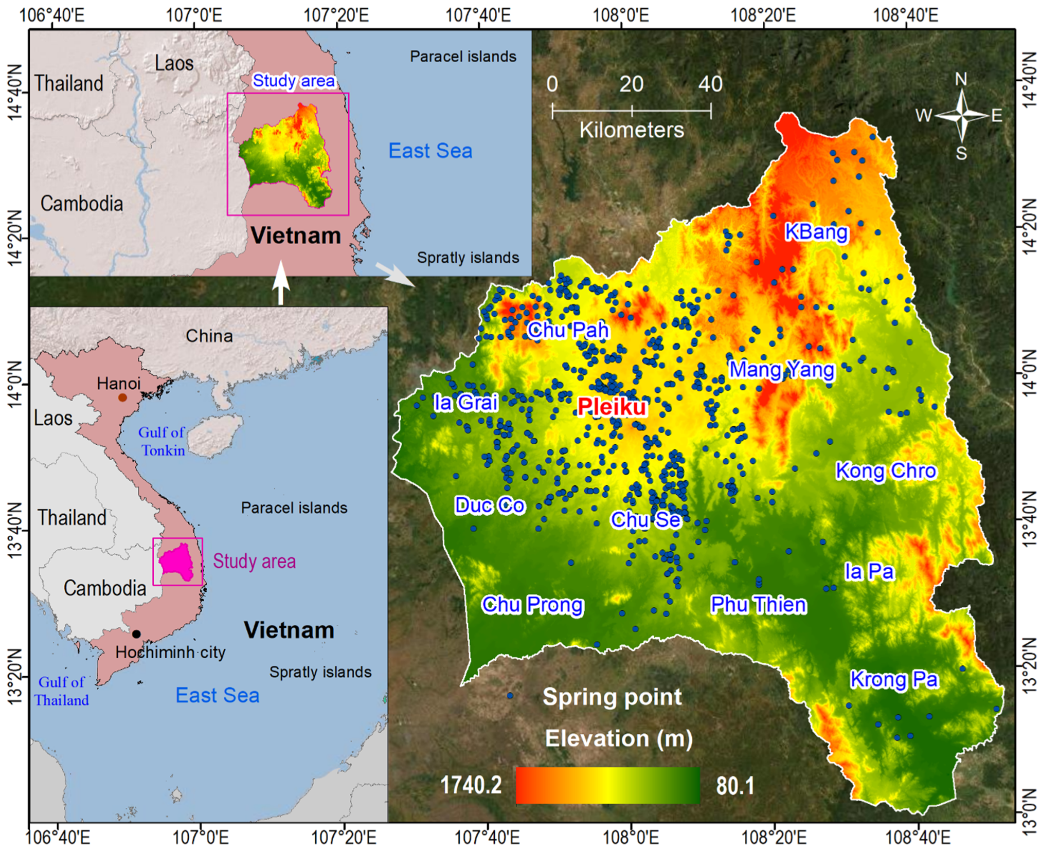
3.1. Study Area

The designated research area pertains to the Gia Lai province, which is positioned in the Central Highlands of Vietnam (Figure 1). It spans across the longitudes of 107°26′E and 108°51′E, and the latitudes of 12°59′N and 14°36′N, with a total land area encompassing 15,512.8 km2 [58]. The province exhibits varying elevations and slopes throughout its terrain. The elevation within the province ranges from 80 m to 1740 m above sea level. Additionally, the region exhibits slopes varying from gentle inclines to steeper angles, with a range spanning from 0.0 to 79.9 degrees. In the province, slopes less than 12.8 degrees play an essential role in forming the largest groundwater springs, constituting over 90% of all spring locations. Specifically, within the slope range of 0–2.5 degrees, approximately 41% of the total spring locations are found, with a flow ranging from 0.01 to 61.27 L per s.
The province is located in the tropical monsoon climate, characterized by distinct wet and dry seasons [59]. Typically, the rainy season extends for approximately seven months, spanning from May to November, while the remaining months constitute the dry season. Our statistical analysis of the climate data POWER project, National Aeronautics and Space Administration (NASA) (www. firms.modaps.eosdis.nasa.gov, accessed on 10 March 2023) in the Gia Lai province from 1981 to 2020 shows that the total rainfall in the rainy season exhibited an enormous variation from 44.83 mm in 1987 to 3114.54 mm in 2020. The highest average monthly temperature ranges from 23.7° in December 1999 to 43.4° in April 2007.
The Gia Lai province is significantly influenced by high temperatures and El Niño [60]. During El Niño events, alterations in precipitation patterns, temperatures, and other meteorological variables have been observed in the province. These alterations have led to increased aridity, decreased rainfall, and higher temperatures, resulting in water shortages, including the depletion of groundwater reserves within the region [61].
The region has experienced robust economic development, marked by significant expansion in coffee and pepper cultivation areas [62]; however, this growth has led to the unsustainable overuse of groundwater resources for irrigation purposes within the region [63]. The region has experienced population growth due to migration, as well as ongoing deforestation carried out by specific ethnic minority groups for agricultural purposes, and consequently, these factors have contributed to a significant depletion of groundwater resources within the region [64].
From a geological perspective, the province exhibits the outcropping of over 40 distinct geological units. Among them, eight units are dominant, which account for 79.64% of the total study area and cover 85.3% of the total groundwater spring locations. They are Tuc Trung formation (25.77%), Van Canh complex (20.02%), BG-QS complex (14.63%), Mang Yang formation (6.48%), Dai Nga formation (4.93%), Lower-Middle Holocene (3.34%), Xa Lam Co formation (2.4%), and Tac Po formation (2.07%) (Table 1). Herein, the primary lithologies encompass tholeiitic olivine basalt, granodiorite, granosyenite, diorite, granite, conglomerate, cobble, and plagioclase. The groundwater spring locations are concentrated in the Tuc Trung formation (68.87%) and Van Canh complex (8.21%). Notably, the Xuan Loc formation (refer to Figure 2 and Table 1) occupies merely 1.55% of the overall study area; however, it contributes to 9.58% of the total groundwater spring locations. The impact of tectonic faults on groundwater springs is not fully discernible, as the majority of springs (83% of the total) are situated more than 2400 m away from the fault zones (refer to Figure 2).

3.2. Groundwater Spring Locations

In the spatial prediction of groundwater springs, an underlying assumption is made that the geo-environmental characteristics of existing springs play a vital role in predicting the potential distribution of groundwater springs within the areas under consideration. Therefore, the initial step involves collecting and compiling inventories of groundwater springs. It is noted that groundwater is typically stored within aquifers and can be accessed through wells or extracted naturally through springs. Herein, spring denotes geographical locations on the land surface where groundwater is discharged from an aquifer, resulting in a discernible and observable flow [65]. Although in mountainous regions, springs are also commonly found within Quaternary sediments. However, groundwater springs primarily occur in locations where the bedrock is fractured, and the overburden is thin [66].
In order to create the groundwater spring inventory map, fieldwork was carried out in the stated fund project B2021-MDA-12 previously [67,68,69]. To identify the spring locations, handheld GPS devices and national topographic maps at a scale of 1:50,000 were utilized. As a result, a total of 938 groundwater spring locations were surveyed and measured (Figure 1 and Figure 2). The measured water flow at these spring locations varies from 0.01 to 118.35 L per s (L/s), with an average of 2.79 L/s. Moreover, the degree of water mineralization at these sites falls within the range of 0.01 to 0.980 g per L (g/L), which complies with the permissible standards for domestic water supply. There are 66 locations where the water flow exceeds 10 L/s, while 352 locations display a water flow ranging between 1.0 and 10.0 L/s.

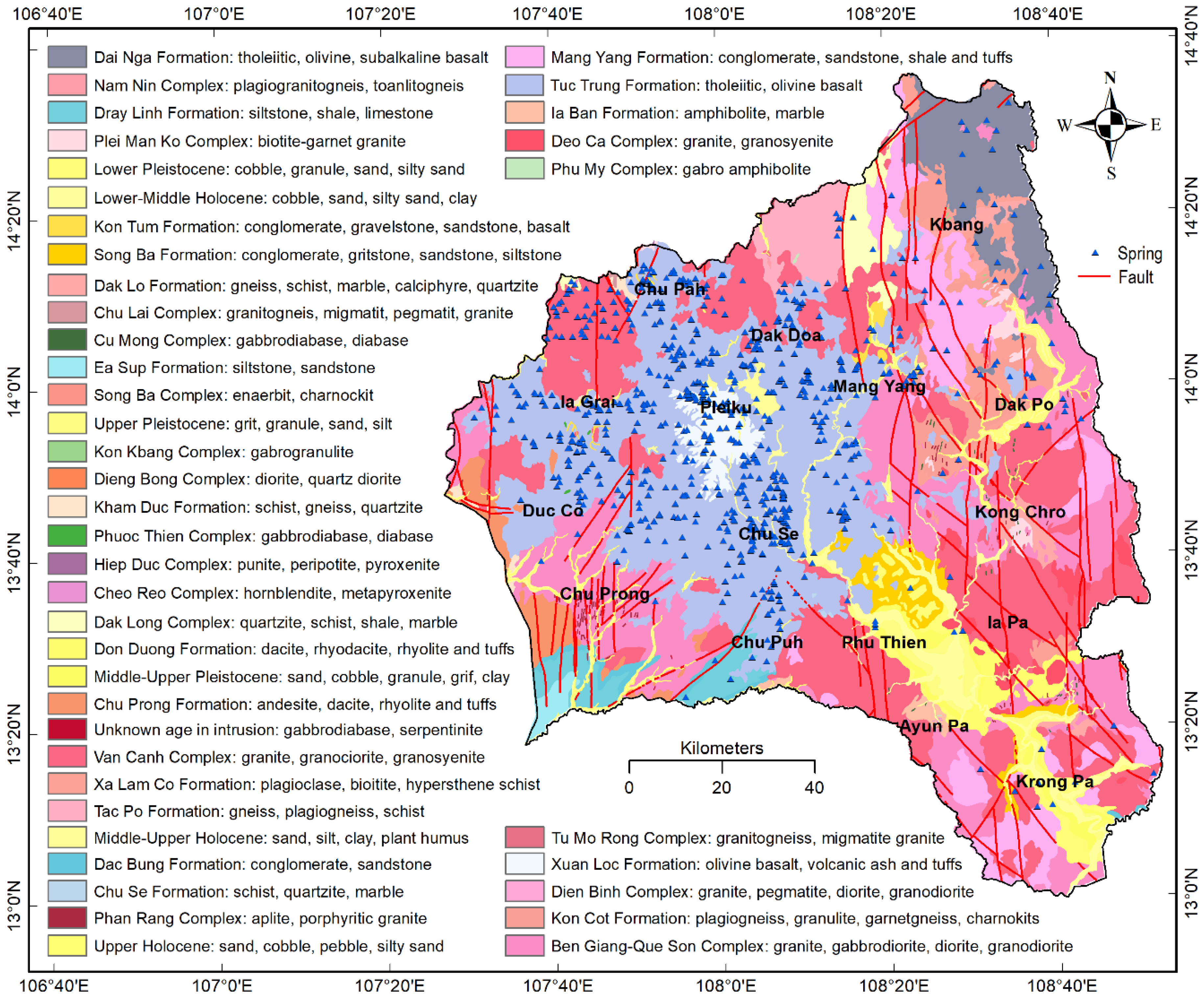
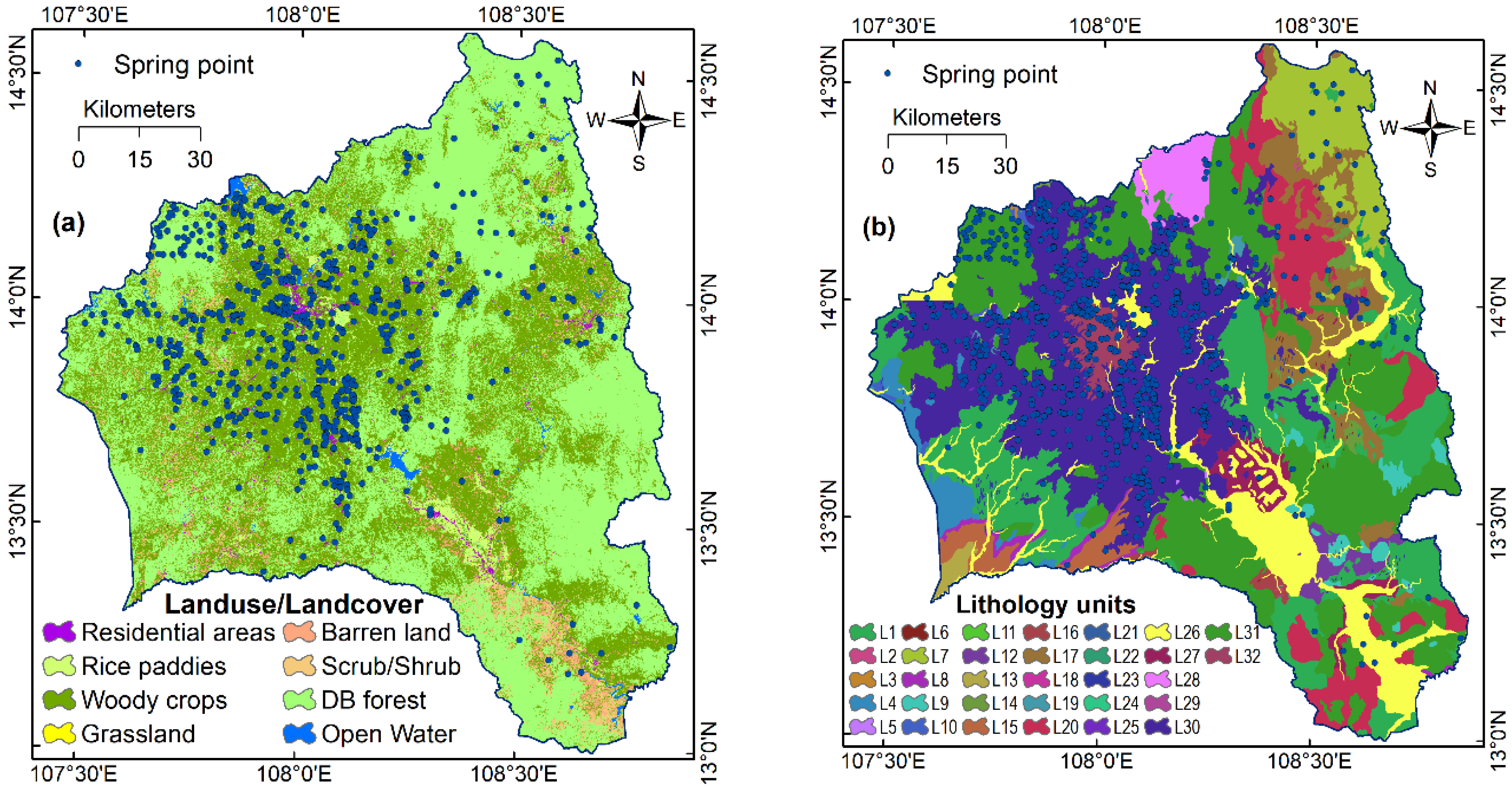
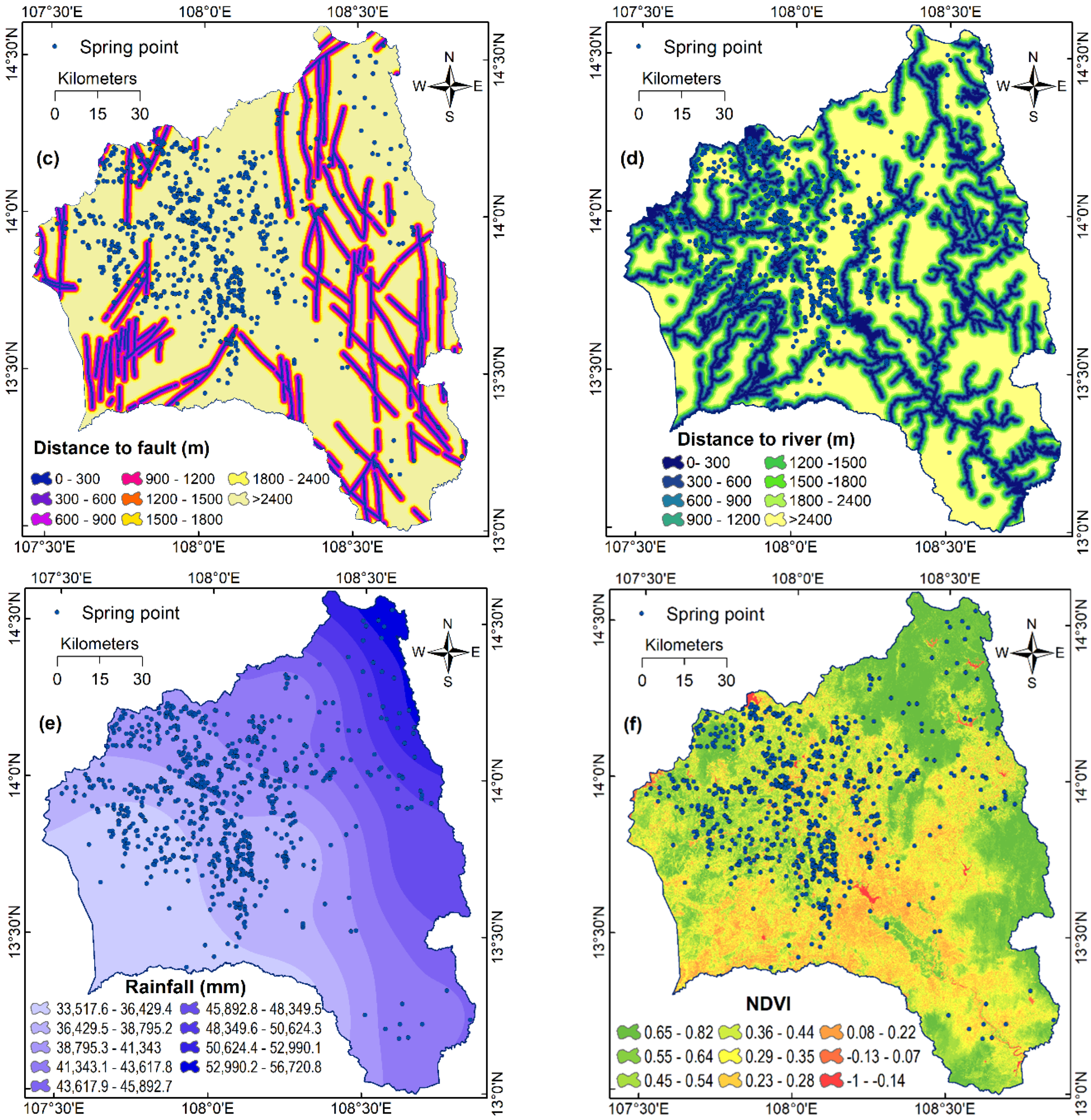
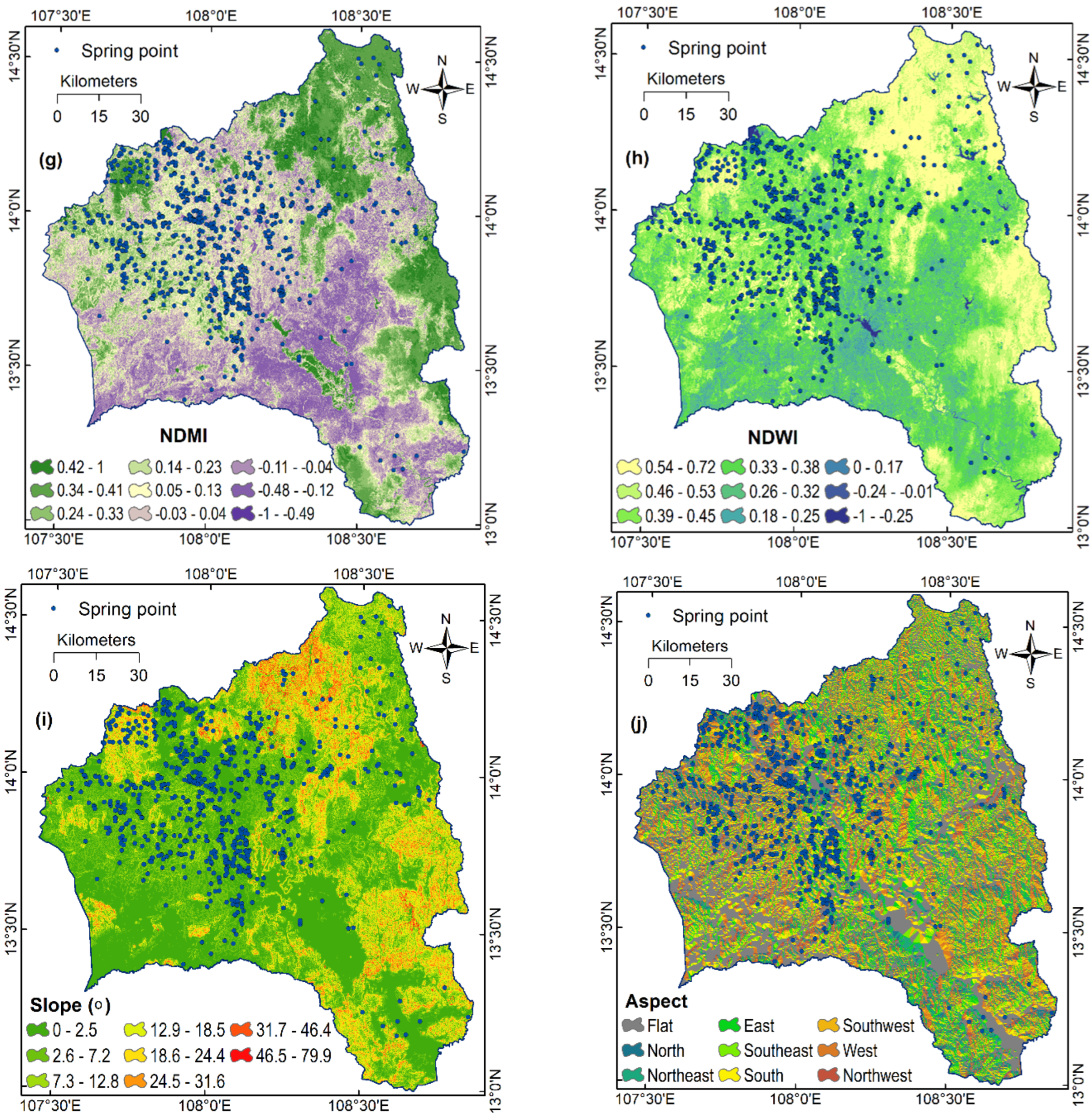
3.3. Groundwater Spring Influencing Factors

The occurrence and movement of groundwater are interconnected with various geo-environmental factors [70], encompassing geology, hydrology, topography, vegetation, and climate [71]. Thus, understanding their influence is crucial for comprehending the behavior of groundwater systems. Based on our analysis of the spring inventory and characteristics of the Gia Lai province, we considered 12 factors: land use and land cover (LULC), geology, distance to fault, distance to river, rainfall, normalized difference vegetation index (NDVI), normalized difference moisture index (NDMI), normalized difference water index (NDWI), slope, aspect, elevation, and curvature.
LULC refers to the activities and vegetation covering the Earth’s surface. Land use refers to human activities and the purpose for which land is utilized, i.e., agriculture, urban development, forestry, or transportation infrastructure [72]. In contrast, land cover, on the other hand, refers to the physical coverage of the Earth’s surface, i.e., vegetation, water bodies, bare soil, and artificial surfaces [73]. LULC is a crucial factor for modeling groundwater spring potential because the types of LULC areas directly influence groundwater recharge, infiltration rates, and the overall hydrological balance [74]. In this analysis, the LULC map with eight groups of the Gia Lai province (Figure 3a) was compiled using the 30 m resolution LULC dataset produced in 2020. This dataset was obtained from the Japan Aerospace Exploration Agency (JAXA) and can be accessed at www.eorc.jaxa.jp. The data retrieval was conducted on 10 March 2023.
Geology plays a crucial role in determining the properties of aquifers, which are underground rock formations that hold and transmit groundwater [65]. Herein, different rock types have varying permeability and porosity, affecting the ability of water to flow through and be stored within the subsurface. Faults should also be considered because they can serve as preferential pathways, enabling water to flow more easily through fractured zones [75]. Moreover, faults can act as barriers, potentially obstructing or diverting the natural flow of groundwater. In this study, the geology map (Figure 3b) for the study area was prepared with 32 classes, whereas the distance-to-fault map with 8 categories (Figure 3c) was constructed by buffering the fault networks of the province. The geological and fault data utilized in this study were obtained from the Geological and Mineral Resources Map at a scale of 1:200,000, which was provided by the Ministry of Natural Resources and Environment of Vietnam.
Distance to river was used in this study because rivers are a significant source of groundwater recharge. Herein, the distance to river relates to the hydraulic connection between the river networks and the groundwater system [76]. Thus, springs that are closer to rivers may have a stronger hydraulic connection. In this study, distance to river with eight classes (Figure 3d) was constructed by buffering the river network using the Multiple Ring Buffer tool in ArcGIS Pro. The river network data used in this study were obtained from OpenStreetMap (www.openstreetmap.org), accessed on 10 March 2023.
Regarding rainfall, this factor is vital for modeling groundwater spring potential due to its direct impact on groundwater recharge, including quantity, distribution, and seasonal variations [77]. Thus, when rainfall occurs, a portion of the water infiltrates into the ground, replenishing the groundwater reservoirs. In this study, the total rainfall data covering the period from 1981 to 2020 in the Gia Lai province were utilized to generate the rainfall map (refer to Figure 3e). The rainfall data were obtained from the POWER project of NASA, as mentioned above.
Remote sensing indices, i.e., NDVI, NDMI, NDWI, have been considered for groundwater studies [78]. NDVI provides information about the presence and vigor of vegetation, which is directly linked to groundwater availability. Higher NDVI values indicate denser vegetation cover, which suggests a higher likelihood of groundwater recharge and sustained spring activity [79]. NDMI is a spectral index that quantifies the moisture content in vegetation and soil. Thus, higher NDMI values indicate a higher soil moisture content [80], which may contribute to groundwater recharge and the presence of springs. NDWI provides an assessment of the moisture availability in the topsoil, indicating potential groundwater recharge zones and areas favorable for spring occurrence [81]. In this analysis, the computation of the remote sensing index maps, NDVI (Figure 3f), NDMI (Figure 3g), and NDWI (Figure 3h) for the Gia Lai province, was performed using the reflectance values obtained from bands 3, 4, 5, and 6 of Landsat 8 OLI imagery at a resolution of 30 m. The calculations were carried out using Equation (7) [82], Equation (8) [83], and Equation (9) [84]. The Landsat 8 OLI imagery can be accessed through the website www.earthexplorer.usgs.gov (accessed on 13 April 2023).
NDVI = (Band 5 − Band 4)/(Band 5 + Band 4)
NDMI = (Band 3 − Band 5)/(Band 3 + Band 5)
NDWI = (Band 5 − Band 6)/(Band 5 + Band 6)
Topographic factors, i.e., slope, aspect, elevation, and curvature, should be considered for groundwater modeling because they influence the movement and distribution of groundwater. Thus, steeper slopes may result in faster runoff and reduced infiltration, potentially affecting groundwater recharge [85], whereas gentle slopes facilitate slower water movement, increasing the likelihood of groundwater retention and the formation of springs. For the case of the aspect, different slope directions may experience varying rates of evapotranspiration [86], affecting the overall water balance and groundwater availability. Elevation relates to a corresponding variation in gravity [71], which significantly influences the potential energy of water and subsequently affects groundwater flow patterns. Herein, changes in elevation may create gradients that drive groundwater movement, including the emergence of springs in lower elevation areas.
In the case of the curvature, this factor quantifies the shape of the land surface that relates to the convergent or divergent flow of water. Herein, areas with concave curvature may accumulate water [87], potentially promoting groundwater recharge and spring formation. Conversely, convex curvature indicates areas where water tends to drain or flow away [88], potentially impacting the occurrence of springs. For this study, the slope map (refer to Figure 3i), aspect map (refer to Figure 3j), elevation map (refer to Figure 3k), and curvature map (refer to Figure 3l) of the Gia Lai province were generated using an ALOS DEM (digital elevation model) at a resolution of 30 m. The ALOS DEM dataset was provided by the Earth Observation Research Center (EORC) of the Japan Aerospace Exploration Agency (JAXA) and can be accessed at www.eorc.jaxa.jp (accessed on 14 April 2023).

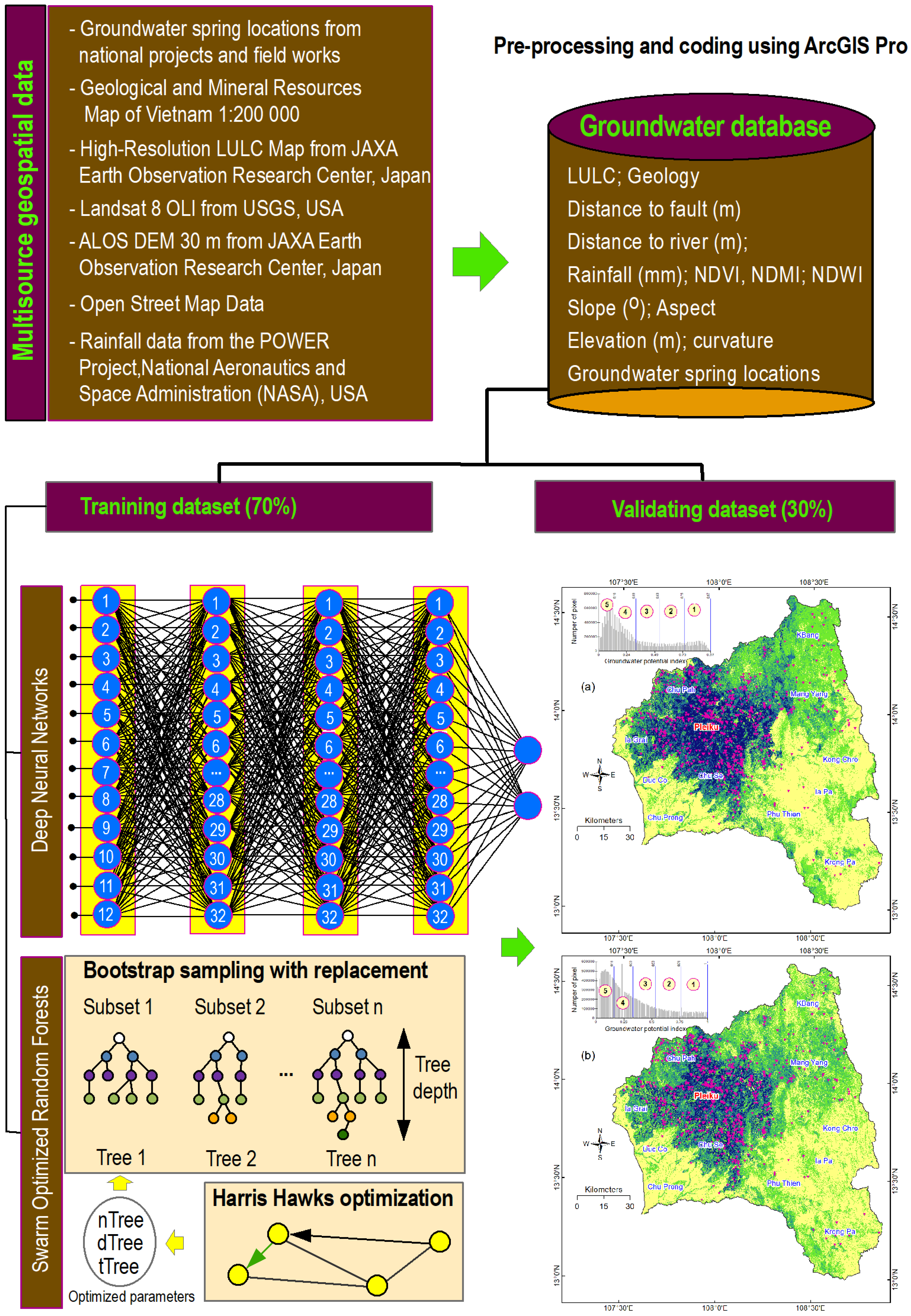
4. Proposed Methodology for Comparative Analysis of Deep Learning and Swarm-Optimized Random Forest for Groundwater Spring Potential Identification

The proposed methodology for predicting the potential locations of groundwater springs using swarm-optimized random forest and deep learning is shown in Figure 4. It is noted that ArcGIS Pro 3.0 with the spatial analysis tool was used to process the multisource geospatial data and build the groundwater database. The Python code for the deep-learning model can be obtained from the official TensorFlow website at www.tensorflow.org (accessed on 10 March 2023). The Matlab code for the Harris Hawks optimization algorithm is available from the work of Heidari, Mirjalili, Faris, Aljarah, Mafarja, and Chen [43]. The author developed the swarm-optimized random forest model (SwarmRF) in the Matlab platform using the Matlab Weka Classifiers tool provided by Dunham (2023). Additionally, a Python script was developed to convert the output of the deep-learning and SwarmRF models into raster format, facilitating the generation of the final groundwater spring potential maps.
  • Step 1. Construction of the groundwater spring database.
In this study, the groundwater spring database for the Gia Lai province was created utilizing the ESRI file geodatabase format. Subsequently, the coordinate system chosen for the study area was WGS 1984 UTM Zone 48N. This coordinate system employs the Transverse Mercator projection with a central meridian of 105°, a scale factor of 0.9996, latitude of origin of 0.0, and a unit of measurement in meters. Next, the groundwater spring inventory map with 938 spring locations and 12 influencing factors were incorporated into the database to ensure uniformity in the coordinate system. Because these factors were generated from multisource geospatial data, this step is crucial for maintaining consistency across the dataset and facilitating modeling during subsequent phases. Then, all factors were converted to a raster format with a spatial resolution of 30 m. Subsequently, all influencing factors were normalized within the range of 0.01 to 0.99 [89]. This normalization process was implemented to mitigate any dominant impact from variations in the magnitude of factor values on the groundwater spring modeling result.
Given that the groundwater spring modeling in this study is framed as a binary pattern recognition problem, a set of 938 nonspring locations were generated outside the groundwater spring areas. Consequently, a total of 1876 locations were obtained. In order to establish training and validation datasets for the study area, these locations were randomly sampled in a 70:30 ratio, resulting in the construction of a training dataset (1314 samples) and a validation dataset (562 samples). Herein, the training and validation datasets were designed to ensure an equal representation of spring and nonspring locations. This approach was adopted to prevent any potential bias in the datasets. The spring locations were assigned “1”, whereas the nonspring locations were assigned “0”. Finally, the value of the 12 influencing factors was extracted for the 2 datasets using the sample tool in ArcGIS Pro.
  • Step 2. Feature selection with the wrapper method.
Selecting appropriate spring influencing factors is vital in groundwater spring modeling and prediction, as it allows for the identification of the most relevant and informative factors. By including only the pertinent spring factors in the model, the performance and accuracy of the model can be significantly enhanced. It helps mitigate the introduction of noise or unnecessary complexity that may arise from irrelevant or redundant spring factors, thereby preventing overfitting and maintaining the overall performance of the models at a higher level.
In this analysis, the wrapper method, which was introduced by Kohavi and John [90], was used due to its efficiency in various prediction domains [91]. Herein, the wrapper method offers a significant advantage by considering the dependencies among input factors, which encompass interactions and redundancies. Given that the wrapper method’s effectiveness is contingent upon the choice of classifier and evaluation metrics, we have opted to utilize the random forest algorithm as the classifier in this study. Furthermore, we have selected mean absolute error (MAE) as the evaluation metric, following the suggestion of Liu and Wang [92].
M A E = 1 n   i = 1 n O p i T g i
where O p i is the output value of the groundwater spring model, whereas T g i is the target value of the groundwater spring in the groundwater spring database; n represents the total number of samples utilized.
  • Step 3. Groundwater spring potential modeling with deep learning.
The architecture of the deep neural network (DNN) model employed in this study comprised 12 input neurons, 3 hidden layers, each containing 32 neurons, and 2 output neurons (refer to Figure 4). The rectified linear unit (ReLU) activation function was chosen, while the sigmoid transfer function was utilized, whereas the Adaptive Moment Estimation (ADAM) optimizer [93], known for its efficiency, was employed, as it has demonstrated effectiveness in recent studies (Bui et al., 2020 [44]). As a result, a total of 2561 parameters were identified for the training process. Mean squared error (MSE) (Equation (11)) was used as an objective function to measure the overall performance of each combination.
M S E = 1 n   i = 1 n ( O p i T g i ) 2
where O p i is the output value of the DNN model, whereas T g i is the target value of the groundwater spring in the groundwater spring database; n represents the total number of samples utilized.
  • Step 4. Groundwater spring potential modeling with swarm-optimized random forest.
In this work, the swarm-optimized random forest (SwarmRF) was employed, where three parameters, the maximum depth of the tree (dTree), the number of randomly chosen features (fTree), and the number of trees in the random forest (nTree), were searched and optimized using the Harris Hawks Optimizer (HHO) algorithm. For this task, the mean squared error (MSE) from Equation (4) was chosen as the cost function to evaluate the model’s performance across various combinations of the three parameters. In this context, a lower MSE value indicates a higher level of model performance.
The configuration parameters for the HHO algorithm in this study were set as follows: a population size of 30 hawks and a total of 1000 iterations. The searching space was defined as follows: for the maximum depth of the tree (dTree), the range was set as [1–100], indicating a maximum tree depth of 100; for the number of trees (nTree) used in the random forest (RF), the range was set as [1–1000], allowing for a maximum of 1000 trees in the RF; and for the number of randomly chosen factors in each tree, the range was set as [1–12], signifying that the algorithm considered a selection from 1 to 12 factors in each individual tree.
  • Step 5. Performance assessment.
In evaluating the performance of the groundwater spring models, widely used statistical metrics for binary classification were employed. These metrics consisted of classification accuracy (Acc), receiver operating characteristic (ROC) curve analysis, area under the curve (AUC), and kappa coefficient. In addition, the positive predictive value (PPV), the negative predictive value (NPV), F-score, sensitivity, and specificity were also included. Detailed explanations of these metrics can be found abundantly in the literature, such as in the work, i.e., of Msaddek et al. [94]. Hence, to prevent redundancy, we have chosen not to delve into a detailed explanation of these metrics in this context. Interested readers are kindly referred to relevant articles for a more comprehensive description of these evaluation metrics.

5. Results and Analysis

5.1. Variable Importance

The outcomes of the feature selection process, conducted using the wrapper method with 5-fold cross-validation, are presented in Table 2. The results highlight the significant role of geology in influencing groundwater spring occurrence within the Gia Lai province, as it achieved the highest-ranking score of 0.250. Following geology, elevation (0.181), NDVI (0.179), NDMI (0.169), LULC (0.153), rainfall (0.151), distance to fault (0.120), and NDWI (0.115) were observed to contribute to the groundwater spring potential. Conversely, curvature exhibited the lowest contribution, with a ranking score of 0.049. Notably, all factors demonstrated relevance and informative value for groundwater spring analysis. Thus, none of them were excluded from this investigation.

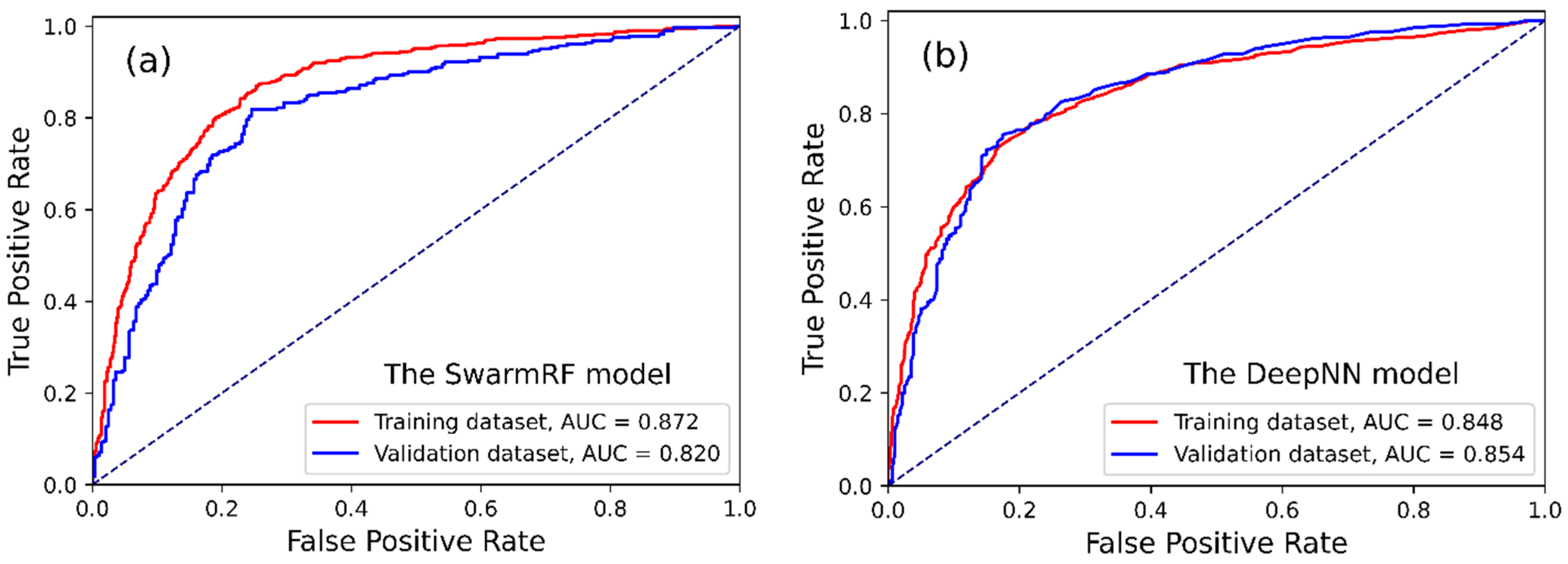
5.2. Model Training and Validation

Using the training dataset with 1314 samples, the DeepNN model was trained in the training phase, where the ADAM algorithm optimized 2561 parameters. The findings are presented in Table 3 and Figure 5, which demonstrate a strong alignment between the DeepNN model and the training dataset. Specifically, the accuracy (Acc) is 80.7%, the F-score is 0.819, the kappa value is 0.615, and the area under the curve (AUC) is 0.872. Furthermore, the positive predictive value (PPV) of 86.9% indicates that the DeepNN model accurately classifies groundwater spring locations in 86.9% of cases. Conversely, the negative predictive value (NPV) of 74.6% signifies the model’s ability to identify nonspring locations in 74.6% of instances correctly. The validation dataset, consisting of 562 samples, was utilized to validate the DeepNN model. The performance of the DeepNN model is displayed in Table 3, revealing commendable results. The recorded metrics for the DeepNN model are as follows: an accuracy (Acc) of 77.9%, an F-score of 0.783, a kappa value of 0.559, and an area under the curve (AUC) of 0.820. Moreover, the positive predictive value (PPV) is 79.7%, signifying the model’s ability to accurately classify groundwater spring locations, while the negative predictive value (NPV) is 76.2%, indicating its proficiency in correctly identifying nonspring locations.
In the case of the SwarmRF model, the parameters dTree, fTree, and nTree underwent optimization using the HHO algorithm with 1000 iterations. The optimal values obtained for these parameters were found to be dTree = 21, fTree = 4, and nTree = 91. By using these parameters, the model was run again using the training dataset with 10-fold cross-validation. The outcomes are presented in Table 3, demonstrating a substantial fit between the model and the training data. Specifically, the accuracy (Acc) achieved a value of 77.9%, the F-score attained 0.777, the kappa coefficient reached 0.557, and the area under the curve (AUC) was measured at 0.839. Additionally, the PPV of 77.2% signifies the DeepNN model’s accurate classification of groundwater spring locations, while the NPV of 78.5% highlights its precise classification of nonspring locations. The validation results indicate that the SwarmRF model demonstrates a high prediction power when applied to the new dataset. The Acc is recorded at 80.2%, the F-score reaches 0.798, the kappa coefficient attains 0.605, and the area under the curve (AUC) is measured as 0.854. Moreover, the PPV of 77.9% confirms the SwarmRF model’s accurate classification of new groundwater spring locations, while the NPV of 82.6% underscores its precise classification of newly nonspring locations.
For the purpose of comparison, the random forest (RF) model was utilized with default parameters. The parameter values were set as follows: dTree was set to unlimited, fTree was randomly selected, and nTree was set to 100. The results presented in Table 3 demonstrate a strong alignment between the model and the training data, with an accuracy (Acc) of 78.2%, an F-score of 0.782, a kappa coefficient of 0.565, and an area under the curve (AUC) of 0.843. Furthermore, the validation results indicate that the RF model yields a favorable prediction performance, with an accuracy (Acc) of 77.8%, an F-score of 0.769, a kappa coefficient of 0.555, and an AUC of 0.840. It could be seen that the prediction performance of the RF model is slightly lower than that of the SwarmRF model.

5.3. Statistical Test

Based on the training and validation results described earlier, it was observed that the SwarmRF model exhibits marginally superior predictive capabilities compared to the DeepNN model, as indicated in Table 3. In order to determine the statistical significance of this difference, a further analysis was conducted. The Wilcoxon signed-rank test [95] was chosen for this purpose, as it takes into account both the direction and magnitude of the differences between paired observations.
Herein, at a significance level (α) of 5%, the null hypothesis states that there is no notable distinction between the groundwater spring models. In order to evaluate the significance of any disparities, the p-value and z-value are computed. If the p-value is below the predetermined significance level of 0.05 and the z-value surpasses the critical values of −1.96 and +1.96, the null hypothesis must be rejected. In such a scenario, it can be concluded that a significant difference exists in the performance of the groundwater spring models. Table 4 shows that the DeepNN model’s performance is statistically significantly lower than the SwarmRF model. The obtained p-values = 0.011 and the z-value (2.553) exceeded the critical values of ±1.96.

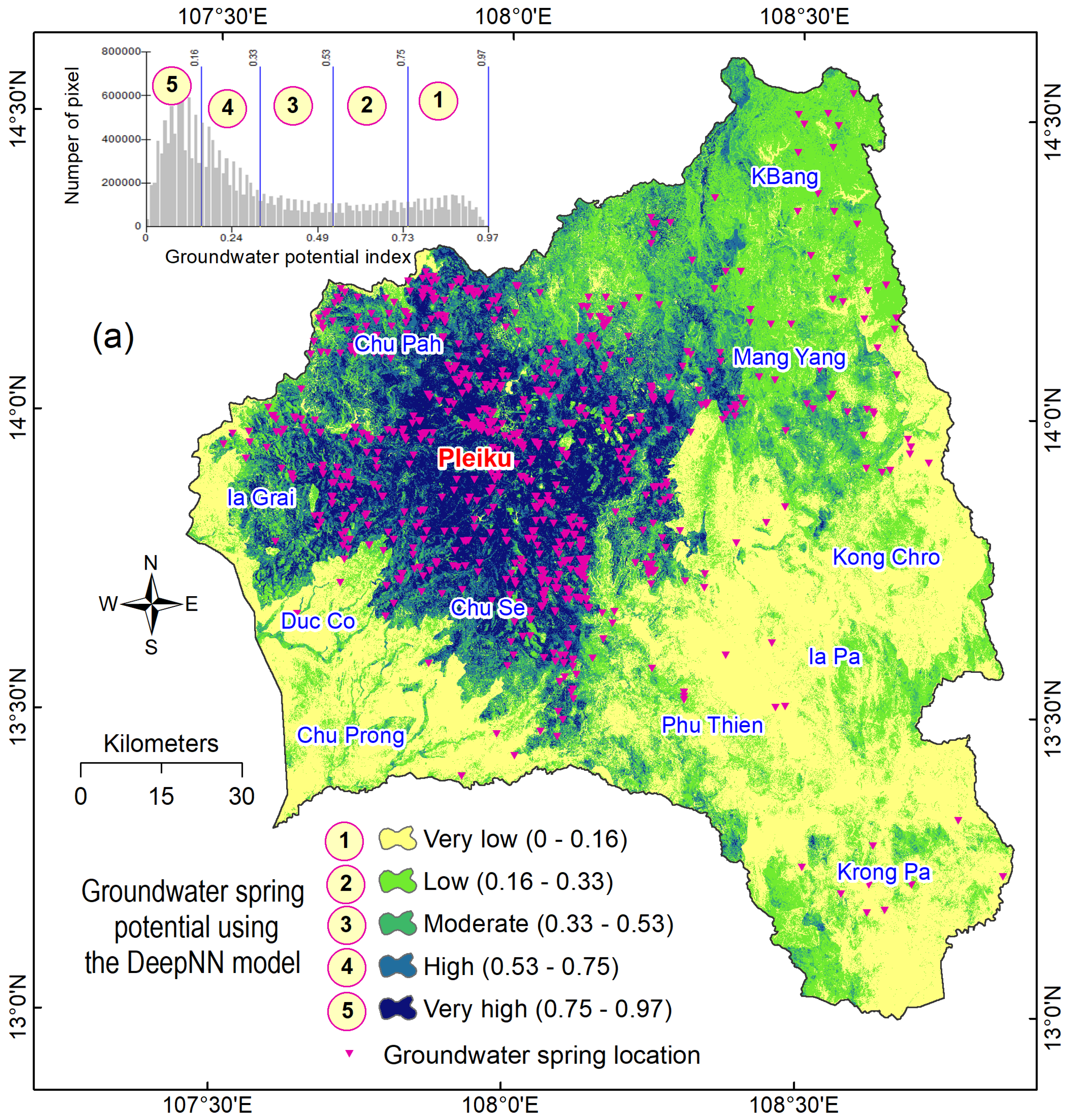
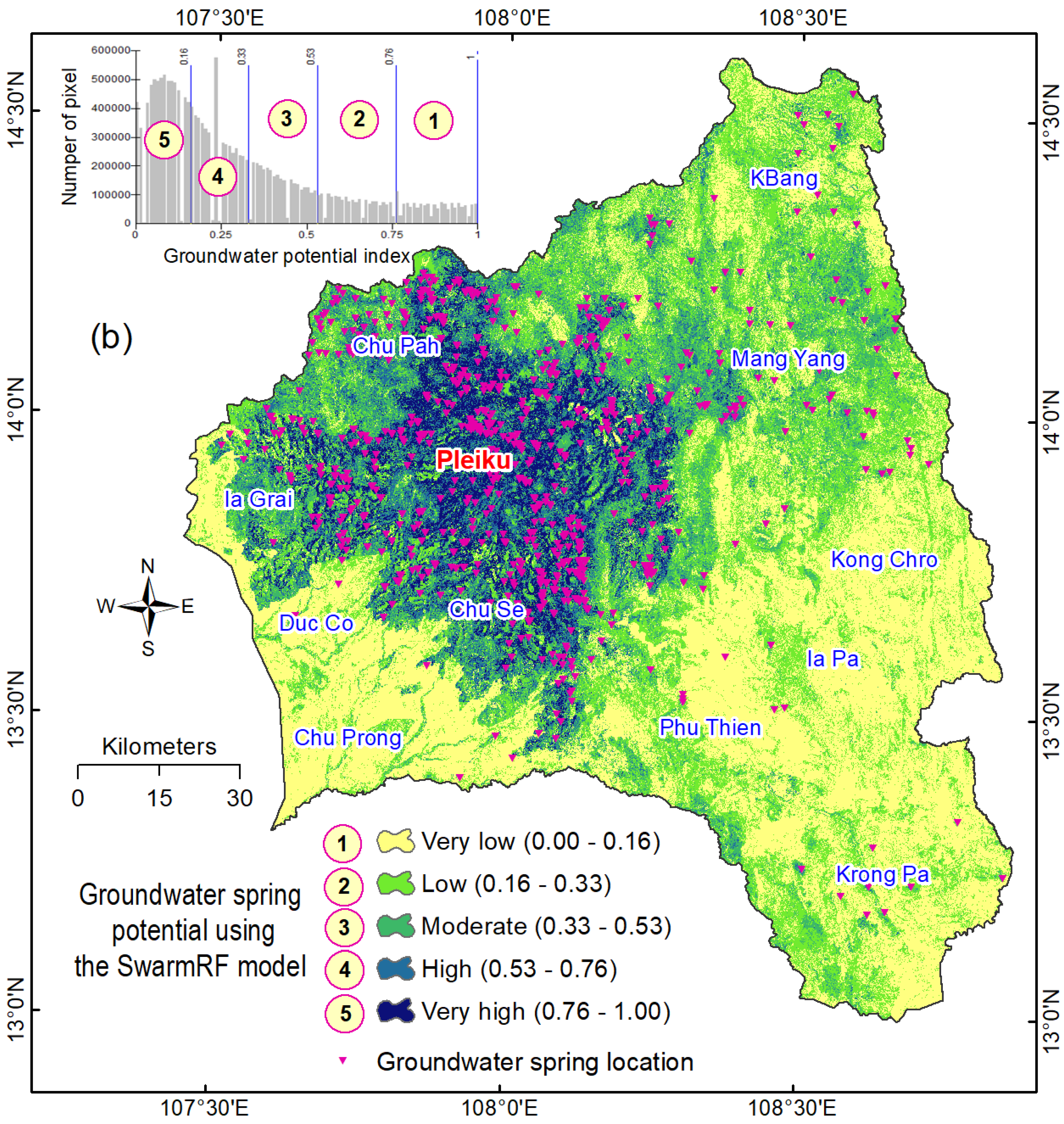
5.4. Compile the Forest Fire Danger Map

In order to compile the groundwater potential maps, the groundwater spring potential (GSP) index for each pixel of the study area was computed using the trained DeepNN model and the trained SwarmRF model. With a resolution of 30 m, the study area was formed by a matrix of 5112 columns × 5934 rows, and as a result, the GSP index for 30,334,608 pixels was computed. The result shows that the potential index value ranges from 0.00 to 0.97 for the DeepNN model (Figure 6a) and from 0.00 to 1.00 for the SwarmRF model (Figure 6b). These indices were reclassified into five classes, very low, low, moderate, high, and very high, using the natural break method available in ArcGIS.
Based on the aerial interpretation of the two maps (Figure 5a,b), it is evident that areas exhibiting high groundwater spring potential are identified within the Pleiku city, the Chu Se district, the Chu Pah district, and the Ia Grai district. These specific regions are situated within the Tuc Trung formation, which is known to harbor a significant number of groundwater spring locations. Conversely, regions such as the Chu Prong district, the Phu Thien district, the Ia Pa district, and the Kong Chro exhibit a relatively low groundwater spring potential.

6. Discussions

The identification of areas with high groundwater spring potential holds paramount importance as it provides invaluable insights for multiple purposes, such as groundwater resource management, land-use planning, and environmental conservation. This significance is particularly pronounced in the context of the Gia Lai province, located in the Central Highlands of Vietnam, which frequently experiences drought crises [96]. Consequently, there is a pressing need to identify the groundwater spring potential using the most accurate prediction model available to address the challenges the region faces effectively. Thus, the comparison between random forest and deep neural networks (DeepNNs), as they are among the most powerful machine-learning techniques for groundwater potential modeling in this study, allows for a comprehensive evaluation of model performance, suitability, generalization, interpretability, and practical considerations. It helps advance the field by identifying the most effective techniques for accurate and reliable predictions, leading to improved decision-making in groundwater management.
The findings of this study indicate that the DeepNN has exhibited remarkable performance. This implies that the DeepNN model has captured complex nonlinear relationships between 12 groundwater spring influencing factors, making them suitable for modeling intricate patterns in groundwater spring data. Thus, with the ADAM optimization, a total of 2561 parameters of the DeepNN model were searched and optimized properly. Even so, the fact that the DeepNN model is still a black-box model makes it challenging to interpret the learned representations of the groundwater spring data. Moreover, it is not easy to understand the reasoning behind the prediction of the groundwater spring potential indices. Unlike the RF, where the decision tree ensemble defines the model structure, deep-learning models have a more flexible and complex architecture. Nevertheless, further work is still required regarding the optimization of the DeepNN model structure.
Concerning the random forest (RF) model, the research findings demonstrate its high predictive capability for groundwater spring potential, showcasing its robustness when applied to multisource geospatial maps. Additionally, the RF model offers ease of interpretation through the utilization of decision trees, which provide clear rules and feature interactions contributing to the final predictions. Furthermore, when combined with the wrapper method, the RF model effectively quantifies the importance of influencing factors on groundwater spring potential. However, it is important to note that the RF model’s performance is sensitive to its parameters, including the number of trees in the random forest (nTree), the maximum depth of the tree (dTree), and the number of randomly chosen features (fTree). The research findings indicate that using the default parameters does not yield the best model prediction, emphasizing the need for parameter optimization to achieve optimal results.
Consequently, through the utilization of the Harris Hawks Optimizer (HHO), the performance of the RF model has been improved and demonstrated a slight superiority compared to the DeepNN model. This is because the SwarmRF facilitates the extraction of feature importance scores, aiding in identifying the most influential variables driving groundwater potential. This interpretable feature analysis is challenging to achieve with DeepNN, making the former more insightful for groundwater prediction tasks. The finding in this study contrasts with the results documented by Wang, Wang, and Han [42], where the RF model’s performance was reported to be lower than that of deep-learning models. However, it is worth noting that there is no clarity regarding the optimization of RF parameters in their study.
Geology is the most important factor among the 12 groundwater spring influencing factors. This is a reasonable result because, in the Gia Lai province, the groundwater springs are mainly located in the Tuc Trung formation. The main lithologies are tholeiitic basalt and subalkaline olivine basalt, with a 30–350 m thickness. They are types of basaltic magma rocks that favor groundwater spring occurrence due to their specific characteristics, i.e., porosity, permeability, and fracture networks [97]. Herein, porosity refers to the presence of void spaces within the rock, while permeability refers to the ability of the rock to transmit water [98]. The interconnected pores and fractures in these basaltic rocks provide pathways for water to flow and accumulate, facilitating the formation of groundwater springs. According to Wu et al. [99], basaltic magma rocks often possess well-developed fracture networks due to the cooling and solidification processes during volcanic activity. The fractures in tholeiitic basalt and subalkaline olivine basalt serve as preferential pathways for groundwater to percolate through the rock and eventually discharge as springs.
Elevation and NDVI are other important factors in this study area. This is primarily due to the fact that the majority of spring locations are concentrated within an elevation range of 300 m to 800 m, comprising 88.3% of the total number of spring locations. Elevation significantly influences the formation of springs by affecting the potential energy of groundwater. Notably, this elevation range also corresponds to the concentration of tholeiitic basalt and subalkaline olivine basalt, as previously mentioned. As for NDVI, 87.8% of the spring locations fall within the NDVI range of 0.30 to 0.8, indicating a strong connection between vegetation distribution and groundwater in this study area.

7. Concluding Remarks

Based on the findings presented, we have reached the following conclusions:
Both deep neural networks and random forests have been identified as powerful methods for the spatial prediction of groundwater spring potential.
The random forests model optimized by the HHO algorithm (referred to as SwarmRF) exhibits a slight superiority in terms of prediction capability compared to the deep neural network (DeepNN) model.
Geology stands out as the most influential factor contributing to groundwater potential mapping.

Author Contributions

Conceptualization: V.-H.N., P.V.H. and D.T.B.; methodology: V.-H.N., P.V.H., L.M.-G. and D.T.B.; validation, V.-H.N. and D.T.B.; writing—original draft preparation: V.-H.N., P.V.H., L.M.-G. and D.T.B.; writing—review and editing: V.-H.N., P.V.H., L.M.-G. and D.T.B. All authors have read and agreed to the published version of the manuscript.

Funding

This work was financially supported by the Ministry of Education and Training (MoET) in Vietnam under grant number B2021-MDA-12.

Data Availability Statement

The data presented in this study are available on request from the corresponding author. The data are not publicly available due to privacy.

Conflicts of Interest

The authors declare no conflict of interest.

References

  1. Famiglietti, J.S. The global groundwater crisis. Nat. Clim. Chang. 2014, 4, 945–948. [Google Scholar] [CrossRef]
  2. Wang, T.; Wu, Z.; Wang, P.; Wu, T.; Zhang, Y.; Yin, J.; Yu, J.; Wang, H.; Guan, X.; Xu, H.; et al. Plant-groundwater interactions in drylands: A review of current research and future perspectives. Agric. For. Meteorol. 2023, 341, 109636. [Google Scholar] [CrossRef]
  3. Fan, Y.; Miguez-Macho, G.; Jobbágy, E.G.; Jackson, R.B.; Otero-Casal, C. Hydrologic regulation of plant rooting depth. Proc. Natl. Acad. Sci. USA 2017, 114, 10572–10577. [Google Scholar] [CrossRef] [PubMed]
  4. Bierkens, M.F.; Wada, Y. Non-renewable groundwater use and groundwater depletion: A review. Environ. Res. Lett. 2019, 14, 063002. [Google Scholar] [CrossRef]
  5. Avila Velasquez, D.I.; Pulido-Velazquez, M.; Hector, M.-S. Improvement of water management for irrigation in Mediterranean basins combining remote sensing, weather forecasting, and artificial intelligence. In Proceedings of the Online Youth Water Congress: “Emerging Water Challenges since COVID-19”, Online, 6–8 April 2022; p. 58. [Google Scholar]
  6. Amadori, M.; Zamparelli, V.; De Carolis, G.; Fornaro, G.; Toffolon, M.; Bresciani, M.; Giardino, C.; De Santi, F. Monitoring Lakes Surface Water Velocity with SAR: A Feasibility Study on Lake Garda, Italy. Remote Sens. 2021, 13, 2293. [Google Scholar] [CrossRef]
  7. Sentas, A.; Karamoutsou, L.; Charizopoulos, N.; Psilovikos, T.; Psilovikos, A.; Loukas, A. The use of stochastic models for short-term prediction of water parameters of the Thesaurus dam, River Nestos, Greece. Proceedings 2018, 2, 634. [Google Scholar]
  8. Jasechko, S.; Seybold, H.; Perrone, D.; Fan, Y.; Kirchner, J.W. Widespread potential loss of streamflow into underlying aquifers across the USA. Nature 2021, 591, 391–395. [Google Scholar] [CrossRef] [PubMed]
  9. Dalin, C.; Wada, Y.; Kastner, T.; Puma, M.J. Groundwater depletion embedded in international food trade. Nature 2017, 543, 700–704. [Google Scholar] [CrossRef]
  10. Scanlon, B.R.; Fakhreddine, S.; Rateb, A.; de Graaf, I.; Famiglietti, J.; Gleeson, T.; Grafton, R.Q.; Jobbagy, E.; Kebede, S.; Kolusu, S.R. Global water resources and the role of groundwater in a resilient water future. Nat. Rev. Earth Environ. 2023, 4, 87–101. [Google Scholar] [CrossRef]
  11. Baghban, S.; Bozorg-Haddad, O.; Berndtsson, R. Water security. In Water Resources: Future Perspectives, Challenges, Concepts and Necessities; IWA Publishing: London, UK, 2021; p. 205. [Google Scholar]
  12. He, C.; Liu, Z.; Wu, J.; Pan, X.; Fang, Z.; Li, J.; Bryan, B.A. Future global urban water scarcity and potential solutions. Nat. Commun. 2021, 12, 4667. [Google Scholar] [CrossRef]
  13. Chenini, I.; Mammou, A.B. Groundwater recharge study in arid region: An approach using GIS techniques and numerical modeling. Comput. Geosci. 2010, 36, 801–817. [Google Scholar] [CrossRef]
  14. Saravanan, R.; Balamurugan, R.; Karthikeyan, M.S.; Rajkumar, R.; Anuthaman, N.G.; Navaneetha Gopalakrishnan, A. Groundwater modeling and demarcation of groundwater protection zones for Tirupur Basin—A case study. J. Hydro-Environ. Res. 2011, 5, 197–212. [Google Scholar] [CrossRef]
  15. Corsini, A.; Cervi, F.; Ronchetti, F. Weight of evidence and artificial neural networks for potential groundwater spring mapping: An application to the Mt. Modino area (Northern Apennines, Italy). Geomorphology 2009, 111, 79–87. [Google Scholar] [CrossRef]
  16. Mogaji, K.; Omosuyi, G.; Adelusi, A.; Lim, H. Application of GIS-based evidential belief function model to regional groundwater recharge potential zones mapping in hardrock geologic terrain. Environ. Process. 2016, 3, 93–123. [Google Scholar] [CrossRef]
  17. Ozdemir, A. Using a binary logistic regression method and GIS for evaluating and mapping the groundwater spring potential in the Sultan Mountains (Aksehir, Turkey). J. Hydrol. 2011, 405, 123–136. [Google Scholar] [CrossRef]
  18. Golkarian, A.; Naghibi, S.A.; Kalantar, B.; Pradhan, B. Groundwater potential mapping using C5.0, random forest, and multivariate adaptive regression spline models in GIS. Environ. Monit. Assess. 2018, 190, 149. [Google Scholar] [CrossRef] [PubMed]
  19. Machiwal, D.; Jha, M.K.; Mal, B.C. Assessment of groundwater potential in a semi-arid region of India using remote sensing, GIS and MCDM techniques. Water Resour. Manag. 2011, 25, 1359–1386. [Google Scholar] [CrossRef]
  20. Arulbalaji, P.; Padmalal, D.; Sreelash, K. GIS and AHP techniques based delineation of groundwater potential zones: A case study from southern Western Ghats, India. Sci. Rep. 2019, 9, 2082. [Google Scholar] [CrossRef] [PubMed]
  21. Pham, Q.B.; Tran, D.A.; Ha, N.T.; Islam, A.R.M.T.; Salam, R. Random forest and nature-inspired algorithms for mapping groundwater nitrate concentration in a coastal multi-layer aquifer system. J. Clean. Prod. 2022, 343, 130900. [Google Scholar] [CrossRef]
  22. Bien, T.X.; Jaafari, A.; Van Phong, T.; Trinh, P.T.; Pham, B.T. Groundwater potential mapping in the Central Highlands of Vietnam using spatially explicit machine learning. Earth Sci. Inform. 2023, 16, 131–146. [Google Scholar] [CrossRef]
  23. Bai, Z.; Liu, Q.; Liu, Y. Groundwater potential mapping in hubei region of china using machine learning, ensemble learning, deep learning and automl methods. Nat. Resour. Res. 2022, 31, 2549–2569. [Google Scholar] [CrossRef]
  24. Das, R.; Saha, S. Spatial mapping of groundwater potentiality applying ensemble of computational intelligence and machine learning approaches. Groundw. Sustain. Dev. 2022, 18, 100778. [Google Scholar] [CrossRef]
  25. Ijlil, S.; Essahlaoui, A.; Mohajane, M.; Essahlaoui, N.; Mili, E.M.; Van Rompaey, A. Machine learning algorithms for modeling and mapping of groundwater pollution risk: A study to reach water security and sustainable development (Sdg) goals in a mediterranean aquifer system. Remote Sens. 2022, 14, 2379. [Google Scholar] [CrossRef]
  26. Chen, Y.; Chen, W.; Chandra Pal, S.; Saha, A.; Chowdhuri, I.; Adeli, B.; Janizadeh, S.; Dineva, A.A.; Wang, X.; Mosavi, A. Evaluation efficiency of hybrid deep learning algorithms with neural network decision tree and boosting methods for predicting groundwater potential. Geocarto Int. 2022, 37, 5564–5584. [Google Scholar] [CrossRef]
  27. Hakim, W.L.; Nur, A.S.; Rezaie, F.; Panahi, M.; Lee, C.-W.; Lee, S. Convolutional neural network and long short-term memory algorithms for groundwater potential mapping in Anseong, South Korea. J. Hydrol. Reg. Stud. 2022, 39, 100990. [Google Scholar] [CrossRef]
  28. Sashikkumar, M.; Selvam, S.; Kalyanasundaram, V.L.; Johnny, J.C. GIS based groundwater modeling study to assess the effect of artificial recharge: A case study from Kodaganar river basin, Dindigul district, Tamil Nadu. J. Geol. Soc. India 2017, 89, 57–64. [Google Scholar] [CrossRef]
  29. Goyal, D.; Haritash, A.; Singh, S. A comprehensive review of groundwater vulnerability assessment using index-based, modelling, and coupling methods. J. Environ. Manag. 2021, 296, 113161. [Google Scholar] [CrossRef] [PubMed]
  30. Jaafarzadeh, M.S.; Tahmasebipour, N.; Haghizadeh, A.; Pourghasemi, H.R.; Rouhani, H. Groundwater recharge potential zonation using an ensemble of machine learning and bivariate statistical models. Sci. Rep. 2021, 11, 5587. [Google Scholar] [CrossRef]
  31. Deng, C.; Zhang, Y.; Bailey, R.T. Evaluating crop-soil-water dynamics in waterlogged areas using a coupled groundwater-agronomic model. Environ. Model. Softw. 2021, 143, 105130. [Google Scholar] [CrossRef]
  32. Farhat, B.; Souissi, D.; Mahfoudhi, R.; Chrigui, R.; Sebei, A.; Ben Mammou, A. GIS-based multi-criteria decision-making techniques and analytical hierarchical process for delineation of groundwater potential. Environ. Monit. Assess. 2023, 195, 285. [Google Scholar] [CrossRef]
  33. Tao, H.; Hameed, M.M.; Marhoon, H.A.; Zounemat-Kermani, M.; Salim, H.; Sungwon, K.; Sulaiman, S.O.; Tan, M.L.; Sa’adi, Z.; Mehr, A.D.; et al. Groundwater level prediction using machine learning models: A comprehensive review. Neurocomputing 2022, 489, 271–308. [Google Scholar] [CrossRef]
  34. Zaresefat, M.; Derakhshani, R. Revolutionizing groundwater management with hybrid AI models: A practical review. Water 2023, 15, 1750. [Google Scholar] [CrossRef]
  35. Naghibi, S.A.; Ahmadi, K.; Daneshi, A. Application of support vector machine, random forest, and genetic algorithm optimized random forest models in groundwater potential mapping. Water Resour. Manag. 2017, 31, 2761–2775. [Google Scholar] [CrossRef]
  36. Knoll, L.; Breuer, L.; Bach, M. Large scale prediction of groundwater nitrate concentrations from spatial data using machine learning. Sci. Total Environ. 2019, 668, 1317–1327. [Google Scholar] [CrossRef] [PubMed]
  37. Kumar, S.; Pati, J. Assessment of groundwater arsenic contamination level in Jharkhand, India using machine learning. J. Comput. Sci. 2022, 63, 101779. [Google Scholar] [CrossRef]
  38. Chen, W.; Li, Y.; Tsangaratos, P.; Shahabi, H.; Ilia, I.; Xue, W.; Bian, H. Groundwater Spring Potential Mapping Using Artificial Intelligence Approach Based on Kernel Logistic Regression, Random Forest, and Alternating Decision Tree Models. Appl. Sci. 2020, 10, 425. [Google Scholar] [CrossRef]
  39. Kumari, S.; Kumar, D.; Kumar, M.; Pande, C.B. Modeling of standardized groundwater index of Bihar using machine learning techniques. Phys. Chem. Earth Parts A/B/C 2023, 130, 103395. [Google Scholar] [CrossRef]
  40. Panahi, M.; Sadhasivam, N.; Pourghasemi, H.R.; Rezaie, F.; Lee, S. Spatial prediction of groundwater potential mapping based on convolutional neural network (CNN) and support vector regression (SVR). J. Hydrol. 2020, 588, 125033. [Google Scholar] [CrossRef]
  41. Moughani, S.K.; Osmani, A.; Nohani, E.; Khoshtinat, S.; Jalilian, T.; Askari, Z.; Heddam, S.; Tiefenbacher, J.P.; Hatamiafkoueieh, J. Groundwater spring potential prediction using a deep-learning algorithm. Acta Geophys. 2023. [Google Scholar] [CrossRef]
  42. Wang, Z.; Wang, J.; Han, J. Spatial prediction of groundwater potential and driving factor analysis based on deep learning and geographical detector in an arid endorheic basin. Ecol. Indic. 2022, 142, 109256. [Google Scholar] [CrossRef]
  43. Heidari, A.A.; Mirjalili, S.; Faris, H.; Aljarah, I.; Mafarja, M.; Chen, H. Harris hawks optimization: Algorithm and applications. Future Gener. Comput. Syst. 2019, 97, 849–872. [Google Scholar] [CrossRef]
  44. Tien Bui, D.; Hoang, N.-D.; Martínez-Álvarez, F.; Ngo, P.-T.T.; Hoa, P.V.; Pham, T.D.; Samui, P.; Costache, R. A novel deep learning neural network approach for predicting flash flood susceptibility: A case study at a high frequency tropical storm area. Sci. Total Environ. 2020, 701, 134413. [Google Scholar] [CrossRef] [PubMed]
  45. Truong, T.X.; Nhu, V.-H.; Phuong, D.T.N.; Nghi, L.T.; Hung, N.N.; Hoa, P.V.; Bui, D.T. A New Approach Based on TensorFlow Deep Neural Networks with ADAM Optimizer and GIS for Spatial Prediction of Forest Fire Danger in Tropical Areas. Remote Sens. 2023, 15, 3458. [Google Scholar] [CrossRef]
  46. Mazurowski, M.A.; Buda, M.; Saha, A.; Bashir, M.R. Deep learning in radiology: An overview of the concepts and a survey of the state of the art with focus on MRI. J. Magn. Reson. Imaging 2019, 49, 939–954. [Google Scholar] [CrossRef] [PubMed]
  47. Karamoutsou, L.; Psilovikos, A. Deep Learning in Water Resources Management: Τhe Case Study of Kastoria Lake in Greece. Water 2021, 13, 3364. [Google Scholar] [CrossRef]
  48. Cano, A. A survey on graphic processing unit computing for large-scale data mining. Wiley Interdiscip. Rev. Data Min. Knowl. Discov. 2018, 8, e1232. [Google Scholar] [CrossRef]
  49. Liu, M.; Wu, W.; Gu, Z.; Yu, Z.; Qi, F.; Li, Y. Deep learning based on batch normalization for P300 signal detection. Neurocomputing 2018, 275, 288–297. [Google Scholar] [CrossRef]
  50. Breiman, L. Random forests. Mach. Learn. 2001, 45, 5–32. [Google Scholar] [CrossRef]
  51. Santos, K.; Dias, J.P.; Amado, C. A literature review of machine learning algorithms for crash injury severity prediction. J. Saf. Res. 2022, 80, 254–269. [Google Scholar] [CrossRef]
  52. Tyralis, H.; Papacharalampous, G.; Langousis, A. A brief review of random forests for water scientists and practitioners and their recent history in water resources. Water 2019, 11, 910. [Google Scholar] [CrossRef]
  53. Speiser, J.L.; Miller, M.E.; Tooze, J.; Ip, E. A comparison of random forest variable selection methods for classification prediction modeling. Expert Syst. Appl. 2019, 134, 93–101. [Google Scholar] [CrossRef] [PubMed]
  54. Wang, X.; Dong, X.; Zhang, Y.; Chen, H. Crisscross Harris hawks optimizer for global tasks and feature selection. J. Bionic Eng. 2023, 20, 1153–1174. [Google Scholar] [CrossRef] [PubMed]
  55. Alabool, H.M.; Alarabiat, D.; Abualigah, L.; Heidari, A.A. Harris hawks optimization: A comprehensive review of recent variants and applications. Neural Comput. Appl. 2021, 33, 8939–8980. [Google Scholar] [CrossRef]
  56. Peng, L.; Cai, Z.; Heidari, A.A.; Zhang, L.; Chen, H. Hierarchical Harris hawks optimizer for feature selection. J. Adv. Res. 2023, in press. [Google Scholar] [CrossRef] [PubMed]
  57. Truong, T.X.; Phuong, N.D.T.; Nghi, L.T.; Nhu, V.-H. A novel HHO-RSCDT ensemble learning approach for forest fire danger mapping using GIS. Vietnam. J. Earth Sci. 2023, 45, 338–356. [Google Scholar]
  58. Le, H.; Bui, Q.; Bui, D.T.; Tran, H.H.; Hoang, N. A Hybrid Intelligence System Based on Relevance Vector Machines and Imperialist Competitive Optimization for Modelling Forest Fire Danger Using GIS. J. Environ. Inform. 2020, 36, 43–57. [Google Scholar] [CrossRef]
  59. Van, N.K.; Ly, P.T.; Hong, N.T. Bioclimatic map of Tay Nguyen at scale 1: 250,000 for setting up sustainable ecological economic models. Vietnam. J. Earth Sci. 2014, 36, 504–514. [Google Scholar] [CrossRef]
  60. Tum, K.; Lai, G.; Lak, D. The Drought Crisis in the Central Highlands of Vietnam; CGIAR Research Program on Climate Change, Agriculture and Food Security (CCAFS): Hanoi, Vietnam, 2016. [Google Scholar]
  61. Tran, T.V.; Bruce, D.; Huang, C.-Y.; Tran, D.X.; Myint, S.W.; Nguyen, D.B. Decadal assessment of agricultural drought in the context of land use land cover change using MODIS multivariate spectral index time-series data. GIScience Remote Sens. 2023, 60, 2163070. [Google Scholar] [CrossRef]
  62. Hiep, N.V.; Ha, N.T.; Thuy, T.T.T.; Van Toan, P. Isolation and selection of Arthrobotrys nematophagous fungi to control the nematodes on coffee and black pepper plants in Vietnam. Arch. Phytopathol. Plant Prot. 2019, 52, 825–843. [Google Scholar] [CrossRef]
  63. Viossanges, M.; Pavelic, P.; Hoanh, C.T.; Vinh, B.; Chung, D.; D’haeze, D.; Dat, L. Linkages between Irrigation Practices and Groundwater Availability: Evidence from the Krong Buk Micro-Catchment, Dak Lak-Vietnam. Final Technical Report. [Contribution to WLE project-Sustainable Groundwater]; International Water Management Institute (IWMI): Colombo, Sri Lanka, 2019. [Google Scholar]
  64. Tam, H.T.; Linh, D.P. How minor immigrants became the dominants: The case of the Kinh people migrating to the Central Highlands, Vietnam in the twentieth century. Soc. Identities 2022, 28, 608–627. [Google Scholar] [CrossRef]
  65. Kresic, N. Chapter 2—Types and classifications of springs. In Groundwater Hydrology of Springs, Kresic, N., Stevanovic, Z., Eds.; Butterworth-Heinemann: Boston, MA, USA, 2010; pp. 31–85. [Google Scholar] [CrossRef]
  66. Haldorsen, S.; Englund, J.-O.; Kirkhusmo, L.A. Groundwater springs in the Hedmarksvidda mountains related to the deglaciation history. Nor. Geol. Tidsskr. 1993, 73, 234–242. [Google Scholar]
  67. Canh, D.V.; Thuy, N.T.T.; Xuan, N.T.; Luat, N.Q.; Nhan, P.Q.; Binh, D.V.; Hue, T.T.; Nhan, D.D.; Tu, N.T.; Long, D.D.; et al. Research on Scientific Basis and Develop Solutions to Store Rainwater into the Ground for Drought Prevention and Protection of Underground Water Resources in the Central Highlands. No. DTDL.2007G/44; Hanoi University of Mining and Geology: Ha Noi, Vietnam, 2010. [Google Scholar]
  68. Duong, H.H.; Lam, N.X.; Tu, N.T.; Tho, H.M.; Phong, N.T.; Tang, N.X.; Thuan, H.L.; Long, N.L.; Hoan, H.V.; Trinh, T.D.; et al. Research and Propose Models and Technological Solutions to Exploit and Protect Water Sources in Basalt Formations in High-Mountainous and Water-Scarcity Areas in the Central Highlands. No. DTDL.CN-65/15; Vietnam Academy for Water Resources: Ha Noi, Vietnam, 2018. [Google Scholar]
  69. Vinh, P.T.; Hai, D.D.; Thanh, T.T.; Huan, K.V.; Giang, V.N.H.; Huyen, T.D.; Chan, N.D.; Nam, P.C.; Tu, N.T.; Luu, N. Research and Propose Models of Collection and Sustainable Exploitation of Spring Groundwater for High-Mountain and Water-Scarces Areas in the Central Highlands. No. DTDL.CN-64/15; Vietnam Academy for Water Resources: Hanoi, Vietnam, 2018. [Google Scholar]
  70. Ozdemir, A. GIS-based groundwater spring potential mapping in the Sultan Mountains (Konya, Turkey) using frequency ratio, weights of evidence and logistic regression methods and their comparison. J. Hydrol. 2011, 411, 290–308. [Google Scholar] [CrossRef]
  71. Tóth, J. Groundwater as a geologic agent: An overview of the causes, processes, and manifestations. Hydrogeol. J. 1999, 7, 1–14. [Google Scholar] [CrossRef]
  72. Lambin, E.F.; Rounsevell, M.D.; Geist, H.J. Are agricultural land-use models able to predict changes in land-use intensity? Agric. Ecosyst. Environ. 2000, 82, 321–331. [Google Scholar] [CrossRef]
  73. Lazzarini, M.; Molini, A.; Marpu, P.R.; Ouarda, T.B.; Ghedira, H. Urban climate modifications in hot desert cities: The role of land cover, local climate, and seasonality. Geophys. Res. Lett. 2015, 42, 9980–9989. [Google Scholar] [CrossRef]
  74. Jyrkama, M.I.; Sykes, J.F. The impact of climate change on spatially varying groundwater recharge in the grand river watershed (Ontario). J. Hydrol. 2007, 338, 237–250. [Google Scholar] [CrossRef]
  75. Myers, T. Potential contaminant pathways from hydraulically fractured shale to aquifers. Groundwater 2012, 50, 872–882. [Google Scholar] [CrossRef]
  76. Sear, D.; Armitage, P.; Dawson, F. Groundwater dominated rivers. Hydrol. Process. 1999, 13, 255–276. [Google Scholar] [CrossRef]
  77. Scibek, J.; Allen, D. Modeled impacts of predicted climate change on recharge and groundwater levels. Water Resour. Res. 2006, 42, W11405. [Google Scholar] [CrossRef]
  78. Liao, F.; Wang, G.; Yang, N.; Shi, Z.; Li, B.; Chen, X. Groundwater discharge tracing for a large Ice-Covered lake in the Tibetan Plateau: Integrated satellite remote sensing data, chemical components and isotopes (D, 18O, and 222Rn). J. Hydrol. 2022, 609, 127741. [Google Scholar] [CrossRef]
  79. Mandal, U.; Sahoo, S.; Munusamy, S.B.; Dhar, A.; Panda, S.N.; Kar, A.; Mishra, P.K. Delineation of groundwater potential zones of coastal groundwater basin using multi-criteria decision making technique. Water Resour. Manag. 2016, 30, 4293–4310. [Google Scholar] [CrossRef]
  80. Mallick, J.; Talukdar, S.; Ahmed, M. Combining high resolution input and stacking ensemble machine learning algorithms for developing robust groundwater potentiality models in Bisha watershed, Saudi Arabia. Appl. Water Sci. 2022, 12, 77. [Google Scholar] [CrossRef]
  81. Mahato, S.; Pal, S. Groundwater Potential Mapping in a Rural River Basin by Union (OR) and Intersection (AND) of Four Multi-criteria Decision-Making Models. Nat. Resour. Res. 2019, 28, 523–545. [Google Scholar] [CrossRef]
  82. Defries, R.S.; Townshend, J.R.G. NDVI-derived land cover classifications at a global scale. Int. J. Remote Sens. 1994, 15, 3567–3586. [Google Scholar] [CrossRef]
  83. Gao, B.-C. NDWI—A normalized difference water index for remote sensing of vegetation liquid water from space. Remote Sens. Environ. 1996, 58, 257–266. [Google Scholar] [CrossRef]
  84. Xu, H. Modification of normalised difference water index (NDWI) to enhance open water features in remotely sensed imagery. Int. J. Remote Sens. 2006, 27, 3025–3033. [Google Scholar] [CrossRef]
  85. Fauzia; Surinaidu, L.; Rahman, A.; Ahmed, S. Distributed groundwater recharge potentials assessment based on GIS model and its dynamics in the crystalline rocks of South India. Sci. Rep. 2021, 11, 11772. [Google Scholar] [CrossRef]
  86. McVicar, T.R.; Van Niel, T.G.; Li, L.; Hutchinson, M.F.; Mu, X.; Liu, Z. Spatially distributing monthly reference evapotranspiration and pan evaporation considering topographic influences. J. Hydrol. 2007, 338, 196–220. [Google Scholar] [CrossRef]
  87. Khosravi, K.; Panahi, M.; Tien Bui, D. Spatial prediction of groundwater spring potential mapping based on an adaptive neuro-fuzzy inference system and metaheuristic optimization. Hydrol. Earth Syst. Sci. 2018, 22, 4771–4792. [Google Scholar] [CrossRef]
  88. Troch, P.; van Loon, E.; Hilberts, A. Analytical solutions to a hillslope-storage kinematic wave equation for subsurface flow. Adv. Water Resour. 2002, 25, 637–649. [Google Scholar] [CrossRef]
  89. Bui, D.T.; Bui, Q.-T.; Nguyen, Q.-P.; Pradhan, B.; Nampak, H.; Trinh, P.T. A hybrid artificial intelligence approach using GIS-based neural-fuzzy inference system and particle swarm optimization for forest fire susceptibility modeling at a tropical area. Agric. For. Meteorol. 2017, 233, 32–44. [Google Scholar]
  90. Kohavi, R.; John, G.H. Wrappers for feature subset selection. Artif. Intell. 1997, 97, 273–324. [Google Scholar] [CrossRef]
  91. Maldonado, J.; Riff, M.C.; Neveu, B. A review of recent approaches on wrapper feature selection for intrusion detection. Expert Syst. Appl. 2022, 198, 116822. [Google Scholar] [CrossRef]
  92. Liu, W.; Wang, J. Recursive elimination–election algorithms for wrapper feature selection. Appl. Soft Comput. 2021, 113, 107956. [Google Scholar] [CrossRef]
  93. Kingma, D.; Ba, J. Adam: A method for stochastic optimization. In Proceedings of the 3rd International Conference for Learning Representations (ICLR’15), San Diego, CA, USA, 7–9 May 2015; Volume 500. [Google Scholar]
  94. Msaddek, M.H.; Ben Alaya, M.; Moumni, Y.; Ayari, A.; Chenini, I. Enhanced machine learning model to estimate groundwater spring potential based on digital elevation model parameters. Geocarto Int. 2022, 37, 8815–8841. [Google Scholar] [CrossRef]
  95. Woolson, R.F. Wilcoxon signed-rank test. In Wiley Encyclopedia of Clinical Trials; John Wiley & Sons, Inc.: Hoboken, NJ, USA, 2007; pp. 1–3. [Google Scholar]
  96. Van Quang, N.; Thanh, N.H. Local government response capacity to natural disasters in the Central Highlands Provinces, Vietnam. Humanit. Soc. Sci. Commun. 2023, 10, 209. [Google Scholar] [CrossRef]
  97. Hale, M.; Plant, J.A. Drainage Geochemistry; Elsevier: Amsterdam, The Netherlands, 2013. [Google Scholar]
  98. Akhtar, N.; Syakir, M.I.; Anees, M.T.; Qadir, A.; Yusuff, M.S. Characteristics and assessment of groundwater. In Groundwater Management and Resources; IntechOpen: London, UK, 2020. [Google Scholar]
  99. Wu, C.; Gu, L.; Zhang, Z.; Ren, Z.; Chen, Z.; Li, W. Formation mechanisms of hydrocarbon reservoirs associated with volcanic and subvolcanic intrusive rocks: Examples in Mesozoic–Cenozoic basins of eastern China. AAPG Bull. 2006, 90, 137–147. [Google Scholar]
Figure 1. Location of the Gia Lai province and groundwater spring locations.
Remotesensing 15 04761 g001
Figure 2. Geology of the Gia Lai province and groundwater spring locations.
Remotesensing 15 04761 g002
Figure 3. Influencing factors: (a) land use and land cover (LULC); (b) geology; (c) distance to fault (m); (d) distance to river (m); (e) rainfall (mm); (f) normalized difference vegetation index (NDVI); (g) normalized difference moisture index (NDMI); (h) normalized difference water index (NDWI); (i) slope (o); (j) aspect; (k) elevation (m); and (l) curvature.
Remotesensing 15 04761 g003aRemotesensing 15 04761 g003bRemotesensing 15 04761 g003cRemotesensing 15 04761 g003d
Figure 4. Flowchart of the proposed methodology for predicting the potential locations of groundwater springs using swarm-optimized random forest and deep learning.
Remotesensing 15 04761 g004
Figure 5. (a) ROC curve and AUC for (a) the DeepNN model and (b) SwarmRF model.
Remotesensing 15 04761 g005
Figure 6. Groundwater spring potential map for Gia Lai province using: (a) the DeepNN model and (b) the SwarmRF model.
Remotesensing 15 04761 g006aRemotesensing 15 04761 g006b
Table 1. The geological units recognized in the Gia Lai province. BS-QS: Ben Giang-Que Son.
NoGeological UnitsArea (%)Spring
Location (%)
Main Lithologies
1Tuc Trung formation25.7768.87Tholeiitic, olivine basalt
2Van Canh complex20.028.21Granite, granociorite, granosyenite
3BG-QS complex14.632.24Granite, gabbrodiorite, diorite
4Mang Yang formation6.481.17Conglomerate, sandstone, shale, and tuffs
5Dai Nga formation4.931.71Tholeiitic, olivine, subalkaline basalt
6Lower-Middle Holocene3.341.71Cobble, sand, silty sand, clay
7Xa Lam Co formation2.40.75Plagioclase, biotite, hypersthene schist
8Tac Po formation2.070.64Gneiss, plagiogneiss, schist
9Kon Cot formation1.951.17Plagiogneiss, granulite, garnetgneiss, charnokits
10Chu Prong formation1.610Andesite, dacite, rhyolite, and tuffs
11Xuan Loc formation1.559.58Olivine basalt, volcanic ash, and tuffs
12Upper Pleistocene1.530.32Grit, granule, sand, silt
13Dray Linh formation1.520.32Siltstone, shale, limestone
14Song Ba formation1.410.11Conglomerate, gritstone, sandstone, siltstone
15Dak Long complex1.340.32Quartzite, schist, shale, marble
16Upper Holocene1.220.32Sand, cobble, pebble, silty sand
17Lower Pleistocene1.210.21Cobble, granule, sand, silty sand
18Dak Lo formation1.060.11Gneiss, schist, marble, caliphate, quartzite
19Deo Ca complex1.030.11Granite, granosyenite, siltstone
20Middle-Upper Pleistocene0.940.21Sand, cobble, granule, grif, clay
21Others3.991.92Dacite, rhyodacite, conglomerate, sand, silt
Table 2. The role of 12 groundwater spring influencing factors using the wrapper method.
No.Groundwater Spring Influencing FactorRanking Score
1Geology0.250
2Elevation (m)0.181
3NDVI0.179
4NDMI0.169
5LULC0.153
6Rainfall (mm)0.151
7Distance to fault (m)0.120
8NDWI0.115
9Slope (°)0.087
10Aspect0.073
11Distance to river (m)0.062
12Curvature0.049
Table 3. Performance of the DeepNN model, the SwarmRF model, and the RF model in the training phase and the validation phase.
Groundwater Spring Model with 10-Fold Cross-ValidationMeasured Metrics
TPTNFPFNPPVNPVSensSpecAccF-ScoreKappaAUC
Training phase
DeepNN5714908616786.974.677.485.180.70.8190.6150.872
SwarmRF50751615014177.278.578.277.577.90.7770.5570.848
RF51451414314378.278.278.278.278.20.7820.5650.843
Validating phase
DeepNN224214576779.776.277.079.077.90.7830.5590.820
SwarmRF219232624977.982.681.778.980.20.7980.6050.854
RF208229735274.081.580.075.877.80.7690.5550.840
Table 4. Pairwise comparison of the groundwater spring models using Wilcoxon signed-rank test.
No.Pairwise Modelz-Valuep-ValueSignificance
1DeepNN vs. SwarmRF2.5530.011Yes
2DeepNN vs. RF2.1990.028Yes
Disclaimer/Publisher’s Note: The statements, opinions and data contained in all publications are solely those of the individual author(s) and contributor(s) and not of MDPI and/or the editor(s). MDPI and/or the editor(s) disclaim responsibility for any injury to people or property resulting from any ideas, methods, instructions or products referred to in the content.

