Article

Ice Identification with Error-Accumulation Enhanced Neural Dynamics in Optical Remote Sensing Images

1
School of Electronics and Information Engineering, Guangdong Ocean University, Zhanjiang 524025, China
2
State Key Laboratory of Satellite Ocean Environment Dynamics, Second Institute of Oceanography, Ministry of Natural Resources, Hangzhou 310012, China
3
School of Artificial Intelligence and Automation, Huazhong University of Science and Technology, Wuhan 430070, China
*
Author to whom correspondence should be addressed.
Remote Sens. 2023, 15(23), 5555; https://doi.org/10.3390/rs15235555
Submission received: 11 October 2023 / Revised: 24 November 2023 / Accepted: 27 November 2023 / Published: 29 November 2023
(This article belongs to the Section Ocean Remote Sensing)

Abstract

:
Arctic sea ice plays an important role in Arctic-related research. Therefore, how to identify Arctic sea ice from remote sensing images with high quality in an unavoidable noise environment is an urgent challenge to be solved. In this paper, a constrained energy minimization (CEM) method is applied for Arctic sea ice identification, which only requires the target spectrum. Moreover, an error-accumulation enhanced neural dynamics (EAEND) model with strong noise immunity and high computing accuracy is proposed to aid with the CEM method for Arctic sea ice identification. With the theoretical analysis, the proposed EAEND model possesses a small steady-state error in noisy environments. Finally, compared with other existing models, the proposed EAEND model can not only complete sea ice identification in excellent fashion, but also has the advantages of high efficiency and noise immunity.

Graphical Abstract

1. Introduction

With the rise in global warming and technological growth, the Arctic has become a strategically important region for countries around the world and is of great importance in terms of economic and trade flows, military, and tourism [1,2,3]. However, Arctic sea ice, an important factor in the global climate system, is steadily melting [4,5], which affects the ecological and climatic environment of the Arctic region [6,7,8]. From other perspectives, the melting of the Arctic sea ice also facilitates the opening of the Arctic corridor and helps to save trade miles and navigation costs, which has important military and trade implications [9]. In addition, the Arctic is rich in fisheries and mineral resources [10], and thus the opening of the Arctic passage facilitates countries with a high demand for energy to research and exploit the Arctic resources. Consequently, to better plan the Arctic passage and Arctic resource investigation routes, it is particularly important to monitor the distribution of sea ice efficiently and in real-time.
Human monitoring of the Arctic sea ice has a long history, starting from early sledding expeditions [11], continuing to aircraft mapping [12], progressing to the use of submarines, icebreakers [13], unmanned equipment [14], and finally to advanced satellite remote sensing technology [15]. Currently, satellite remote sensing technology is the most efficient way to monitor sea ice, and it has advantages of wide-range detection, real-time, and sustainability differing from traditional methods. It is worth affirming that synthetic aperture radar (SAR) is generally not affected by weather disturbances or cloud cover, which greatly enhances its applicability in acquiring remote sensing imagery [16,17]. However, compared to SAR, optical imagery has some unique advantages in polar research. First, optical remote sensing is one of the most direct methods for satellite remote sensing technology and is able to obtain visible light images and panchromatic images with high spatial resolutions that provide clear spatial texture information of the observation target [18,19,20], which is instrumental in the intuitive interpretation of remote sensing images. Second, the acquisition and processing of optical imagery are relatively more straightforward to operate and analyze. Optical images can be directly obtained for free from satellite platforms. It is worth pointing out that acquiring SAR images often involves significant costs. In the processing of SAR images, due to their unique properties, such as speckle noise and polarization characteristics, these images requires higher computational power and specialized expertise to ensure the accuracy and reliability of the image results. Although the use of optical imagery limits the creation of time series, in the Arctic summer, abundant sunlight and less cloud cover make optical imagery an ideal data source for observing sea ice. Furthermore, due to the intuitiveness of optical imagery, it has unique advantages for real-time monitoring and navigation planning [21]. Based on this, our study aims to propose a rapid and accurate identification method, contributing to the planning of navigation routes and the monitoring of maritime emergencies. Generally speaking, researchers usually adopt three methods for identifying Arctic sea ice: thresholding, texture analysis, and machine learning.
Thresholding initially employed the adaptive global thresholding method that calculates a global threshold by analyzing the grayscale data of the entire image followed by categorizing the pixels into black and white. However, using this method for sea ice images under various lighting conditions is inappropriate, resulting in imprecise segmentation outcomes. To overcome the limitations of global adaptive thresholding, D. Haverkamp et al. [22] introduced the local adaptive thresholding method. This method leverages the neighborhood information of every pixel to calculate its local threshold and categorizes pixels into black and white accordingly. In contrast to the global thresholding method, the local adaptive thresholding method can precisely identify regions of sea ice. Later, Alexander S. Komarov et al. [23] achieved commendable experimental results by detecting ice and open water areas in RADARSAT-2 images using adaptive probability thresholding.
The early texture analysis method was based on the gray-level co-occurrence matrix (GLCM) method. By calculating the grayscale value differences between pixels in the image, this method assesses the texture characteristics of diverse regions. Unfortunately, the GLCM-based method is computationally intensive and requires significant data preprocessing, making it impractical for large-scale remote sensing of sea ice. To overcome the drawbacks of the GLCM-based method, ref. [24] presented an overview of the one-dimensional discrete wavelet transform method leveraging Daubechies wavelet filters represented by finite vectors and matrices. The method takes into account the scale-dependent wavelet variance and covariance and determines their respective confidence intervals. The wavelet transform-based method can handle large-scale remote sensing images of sea ice more quickly than the GLCM-based method.
Numerous machine learning techniques employ hand-crafted feature identification, such as wavelet transform for texture feature identification from images, and using conventional classifiers like support vector machine and decision tree for image segmentation [25]. These methods necessitate manual feature identification, which is subjective and has certain limitations. Advancements in deep learning technology have facilitated the inclusion of machine learning techniques based on convolutional neural networks (CNN) in remote sensing image processing of sea ice. After using substantial remote sensing images and corresponding labelled data to train CNN models, the model is then deployed to categorize new remote sensing images [26]. During the development of machine learning techniques, researchers gradually identify the discrepancy problem between remote sensing image data and ground truth label data. Hence, unsupervised learning methods have emerged, such as generative adversarial networks-based techniques [27,28]. These techniques can categorize remote sensing images of sea ice, even in the absence of labeled data.
Although these three methods have achieved constructive results in the identification of Arctic sea ice, there are still some shortcomings. For example, threshold-based methods are not good at distinguishing thin ice from seawater and are easily affected by light interference. In addition, texture analysis-based methods require classification of different types of sea ice, which requires professional knowledge reserves and experience in acquiring remote sensing images, limiting the technical application scope of such methods. Furthermore, although machine learning methods have achieved good results in image training, they require a large amount of training data and computational resources, as well as the design of professional models, which inevitably consumes a lot of time.
In conclusion, the efficient and accurate identification of Arctic sea ice from remote sensing images is a pressing issue. To approach this problem, a constrained energy minimization (CEM) method is considered [29,30,31], which solely requires the target spectrum without the need for image background information. By employing predetermined constraints, a finite impulse response filter is developed to enable the desired target signal to pass through, while effectively suppressing output energy introduced by secondary signals. CEM is highly versatile and efficient, making it an ideal approach for numerous remote sensing image processing tasks. It is frequently used for identifying various target objects such as land-cover [32], farmland [33], coastal change [34], and so on [35,36,37]. These applications have all yielded impressive results. Despite the CEM method being effective at target identification, it is still susceptible to ambient noise, including unavoidable noises generated from working devices. Consequently, identifying targets using CEM is still restricted by the working environment. To address this shortcoming, this paper proposes utilizing a model that possesses noise immunity to enhance the effectiveness of the CEM method for Arctic sea ice identification.
The CEM method can be transformed into a linear constrained optimization problem. Neural dynamics (ND) shows satisfactory performance in solving optimization problems, such as fast computational speed and good convergence, and has been studied by many scholars [38,39,40,41]. For example, it can be applied to the motion generation and control of redundant manipulators [42], the tracking control of chaotic systems [43], and even to biological population control [44]. In practical applications, continuous models need to be discretized before being applied to hardware devices. This is different from most of the existing ND models that apply Euler difference formulas to discrete continuous models [45,46,47].
This paper applies a Taylor numerical difference formula [48] for discretization, which enables its steady-state error to reach O ( σ 3 ) smaller than that of Euler difference formulas with σ being the sampling period. Additionally, the absence of noise is always a prerequisite for the implementation of some models, but the presence of noise is unavoidable in practical working situations. To this end, a neural dynamics model with an integration term using the Taylor numerical difference formula for discretization, named error-accumulation enhanced neural dynamics (EAEND) model, is proposed to improve the stability and accuracy of the CEM method for Arctic sea ice identification. Thereafter, relevant convergence analysis and stability proofs are provided, which theoretically illustrate the convergence and noise immunity of the CEM method with the proposed EAEND model in noisy environments. Moreover, to assess the effectiveness of the CEM method integrated with the EAEND model for identifying Arctic sea ice, a series of comparative experiments are conducted on various sea ice observation images abiding by different noise environments. The outcomes highlight the superior noise immunity and benefits of incorporating the EAEND model.
Figure 1 illustrates the flowchart representing the CEM method’s process for Arctic sea ice identification assisted by the EAEND model. Specifically, this paper transforms the CEM scheme into an optimization problem. Subsequently, the EAEND model proposed in this paper is used to solve the optimization problem. To minimize the error and obtain an optimal filter coefficient for Arctic sea ice identification, an error function is constructed and the ND formula with an integral term is introduced. The error is then minimized using error-accumulative enhanced neural dynamics. Thus, the Arctic sea ice can be successfully identified.
In the subsequent sections of this paper, the organization is as follows. Section 2 provides the model construction of the EAEND model; Section 3 gives the model simplification as well as theoretical proofs for the convergence and robustness of the EAEND model; Section 4 and Section 5 present comparative identification experiments of different Arctic sea ice remote sensing images, while the proposed EAEND model is compared with other models; in Section 6, the experimental results are discussed and analyzed. Section 7 summarizes the whole paper. The contribution points of this paper are provided below.
  • The proposed EAEND model, using a Taylor numerical difference formula to enable steady-state error to reach O ( σ 3 ) , is capable of improving the Arctic sea ice identification accuracy of the CEM method.
  • The proposed EAEND model eliminates the computing error by using an error integration term, and therefore effectively suppresses noises and improves the solution accuracy, which is able to assist the CEM method in identifying Arctic sea ice in noisy environments.
  • Theoretical analyses and comparative experiments confirm that the CEM method with the proposed EAEND model has high accuracy and strong stability.

2. Problem Formulation

The CEM method is formulated as a quadratic programming problem [49,50] as follows:
min A ( t ) u ( t ) + s ( t ) 2 2 / 2 , s . t . B ( t ) u ( t ) = z ( t ) ,
where · 2 denotes the Euclidean norm; A ( t ) R j × m and B ( t ) R n × m are the full-rank matrices; s ( t ) R j and z ( t ) R n are the coefficient vectors; and u ( t ) R m is the unknown vector to be solved.
To further illustrate the CEM method (1), let f ( u ) = A ( t ) u ( t ) + s ( t ) 2 2 , C ( t ) = A T ( t ) A ( t ) R m × m , and p ( t ) = A T ( t ) s ( t ) R m , with superscript T being the transposition operation. The Lagrange formula is as follows:
L ( u ( t ) , r ( t ) , t ) = f ( u ( t ) , t ) + r ( t ) T ( B ( t ) u ( t ) z ( t ) ) ,
where r ( t ) equals to [ r 1 ( t ) , ⋯, r n ( t ) ] T R n , meaning the Lagrange-multiplier operator vector. The optimal solution of the CEM method (1) satisfies the following equation:
L ( u ( t ) , r ( t ) , t ) u ( t ) = f ( u ( t ) , t ) u ( t ) + B T ( t ) r ( t ) = 0 , L ( u ( t ) , r ( t ) , t ) r ( t ) = B ( t ) u ( t ) z ( t ) = 0 .
Subsequently, for simplicity, let
N ( t ) = C ( t ) B T ( t ) B ( t ) 0 n × n R ( m + n ) × ( m + n ) , x ( t ) = u ( t ) r ( t ) R m + n , g ( t ) = p ( t ) z ( t ) R m + n .
Therefore, (3) is summarized as
N ( t ) x ( t ) = g ( t ) .
For measuring the accuracy of the computing solution, an error function can be defined as follows:
ε ( t ) = N ( t ) x ( t ) g ( t ) .
Then, an ND formula [46] with an error integration term making the error function approach zero is designed as
ε ˙ ( t ) = φ ε ( t ) ϖ 0 t ε ( ϱ ) d ϱ ,
where φ > 0 and ϖ > 0 . Then, associating (5) and (6) yields
N ( t ) x ˙ ( t ) = g ˙ ( t ) N ˙ ( t ) x ( t ) φ N ( t ) x ( t ) g ( t ) ϖ 0 t N ( ϱ ) x ( ϱ ) g ( ϱ ) d ϱ ,
where N ˙ ( t ) , x ˙ ( t ) , and g ˙ ( t ) are the derivatives of N ( t ) , x ( t ) , and g ( t ) , respectively. Then, it can be rearranged as
x ˙ ( t ) = N 1 ( t ) ( g ˙ ( t ) N ˙ ( t ) x ( t ) φ N ( t ) x ( t ) g ( t ) ϖ 0 t N ( ϱ ) x ( ϱ ) g ( ϱ ) d ϱ ) .
Next, in order to approximate the first-order derivatives with high computational accuracy, a three-step forward difference formula [51] employed to discrete model (8) is as follows:
x ˙ k = 2 x k + 1 3 x k + 2 x k 1 x k 2 2 σ ,
where k denotes the updating index at time instant t = k σ and σ is the sampling period. Then, applying the Euler backward-difference formula to approximate N ˙ k and g ˙ k generates the EAEND model:
x k + 1 = 1.5 x k x k 1 + 0.5 x k 2 + N k 1 ( ( g k g k 1 ) ( N k N k 1 ) x k Υ ( N k x k g k ) Γ i = 0 k ( N i x i g i ) ) ,
where Υ = φ σ and Γ = ϖ σ 2 .

3. Theoretical Analysis and Proof

EAEND model (10) has high accuracy performance in noisy environments, and its convergence and stability are analyzed and proved below.

3.1. Model Simplification

In order to facilitate the subsequent analysis of the model, we focus on deriving a simplified neural dynamics model.
Theorem 1.
EAEND model (10) can be rewritten as
ε k + 1 = ( 1.5 Υ ) ε k ε k 1 + 0.5 ε k 2 Γ i = 0 k ε i + O ( σ 3 ) ,
where O ( σ 3 ) denotes the vector of truncation error O ( σ 3 ) .
Proof. 
First, by applying a Taylor numerical difference formula [48], we have
ε ˙ k = 2 ε k + 1 3 ε k + 2 ε k 1 ε k 2 2 σ + O ( σ 2 ) .
Subsitituting the equation above into (6), one can further obtain:
2 ε k + 1 3 ε k + 2 ε k 1 ε k 2 2 σ + O ( σ 2 ) = φ ε k ϖ σ i = 0 k ε i .
Furthermore, (12) can be simplifed as:
ε k + 1 1.5 ε k + ε k 1 0.5 ε k 2 = Υ ε k Γ i = 0 k ε i + σ O ( σ 2 ) .
Then, by simplifying the above formula, the equation can eventually be written as
ε k + 1 = ( 1.5 Υ ) ε k ε k 1 + 0.5 ε k 2 Γ i = 0 k ε i + O ( σ 3 ) .
The proof is complete. □

3.2. Convergence Analysis

This subsection proves the convergence of EAEND model (10) in a noise-free environment.
Theorem 2.
The steady-state computing error lim k ε k 2 of EAEND model (10) is O ( σ 3 ) .
Proof. 
Considering ε k θ as the θ th subsystem of ε k , the θ th subsystem of (14) is written as
ε k + 1 θ = ( 1.5 Υ ) ε k θ ε k 1 θ + 0.5 ε k 2 θ Γ i = 0 k ε i θ + O ( σ 3 ) .
Then, the θ th subsystem of term ε k 1 is
ε k θ = ( 1.5 Υ ) ε k 1 θ ε k 2 θ + 0.5 ε k 3 θ Γ i = 0 k 1 ε i θ + O ( σ 3 ) .
Subtracting (16) from (15) yields
ε k + 1 θ = ( 2.5 Υ Γ ) ε k θ ( 2.5 Υ ) ε k 1 θ + 1.5 ε k 2 θ 0.5 ε k 3 θ + O ( σ 3 ) .
Define Φ k + 1 θ = [ ε k + 1 θ , ε k θ , ε k 1 θ , ε k 2 θ ] T . Then, (17) can be rearranged as
Φ k + 1 θ = P Φ k θ + O ( σ 3 ) ,
with
P = 2.5 Υ Γ ( 2.5 Υ ) 1.5 0.5 1 0 0 0 0 1 0 0 0 0 1 0 .
Then, (18) can be generalized as
Φ k + 1 θ 2 P Φ k θ 2 + O ( σ 3 ) 2 = P Φ k θ 2 + O ( σ 3 ) P 2 Φ k θ 2 + O ( σ 3 ) P 2 P Φ k 1 θ 2 + P 2 O ( σ 3 ) + O ( σ 3 ) = P 2 P Φ k 1 θ 2 + O ( σ 3 ) P 2 2 Φ k 1 θ 2 + O ( σ 3 ) P 2 k Φ 1 θ 2 + O ( σ 3 ) .
The four real parts of the eigenvalues of matrix P are in the range [ 1 , 1 ] , it can be inferred that lim k P 2 k = 0 [51]. Therfore, it has
lim k Φ k + 1 θ 2 lim k P 2 k Φ 1 θ 2 + O ( σ 3 ) = O ( σ 3 ) .
According to the definitions of Φ k + 1 θ and ε k θ , it is easy to conclude that the steady-state computing error lim k ε k 2 is O ( σ 3 ) . The proof is complete. □

3.3. Robustness Analysis

When the machine is working, the noise from the surroundings or the machine itself has a great impact on the data collection. Based on this, a noise perturbation item can be defined as ψ ( t ) . Thus, EAEND model (10) with a noise disturbance item is rerwitten as
x k + 1 = 1.5 x k x k 1 + 0.5 x k 2 + N k 1 ( ( g k g k 1 ) ( N k N k 1 ) x k Υ ( N k x k g k ) Ω i = 0 k ( N i x i g i ) + ψ ( t ) ) .
Then, in order to illustrate the robustness of EAEND model (19) in the aforementioned circumstance, the following theorem is presented.
Theorem 3.
Assuming that EAEND model (19) aiding CEM method (1) for Arctic sea ice identification is affected by the constant noise ψ ( t ) = μ , the steady-state computing error of EAEND model (19) is O ( σ 3 ) , regardless of the magnitude of ψ ( t ) = μ .
Proof. 
EAEND model (10) is converted into a linear system (14), and thus the steady-state computing error of the model is the superposition effects of the constant noise ψ ( t ) = μ and O ( σ 3 ) . Thus, from (14), the θ th subsystem with the constant noise term can be regarded as
ε k + 1 θ = ( 1.5 Υ ) ε k θ ε k 1 θ + 0.5 ε k 2 θ Γ i = 0 k ε i + μ θ .
The aforementioned equation can be converted via the Z-transform into the following form:
z ε θ ( z ) z ε θ ( 0 ) = ( 1.5 Υ ) ε θ ( z ) z 1 ( ε θ ( z ) + z ε θ ( 1 ) ) + 0.5 z 2 ( ε θ ( z ) + z 2 ε θ ( 2 ) + z ε θ ( 1 ) ) Γ ε θ ( z ) 1 z 1 + z μ θ z 1 ,
where ε θ ( 0 ) denotes the initial value of ε θ . The above equation can be further expressed as
( z ε θ ( 0 ) ( 0.5 z 1 1 ) ε θ ( 1 ) + 0.5 ε θ ( 2 ) + z μ θ z 1 ) ε θ ( z ) = z 1.5 + Υ + z 1 0.5 z 2 + z Γ z 1 .
Therefore, the expression about ε θ ( z ) is
ε θ ( z ) = z 3 ( z 1 ) ( ε θ ( 0 ) + z 2 ( 0.5 z ) ε θ ( 1 ) ) z 4 + ( 2.5 + Υ + Γ ) z 3 + ( 2.5 Υ ) z 2 1.5 z + 0.5 + z 3 ( z 1 ) ( 0.5 z 1 ε θ ( 2 ) + ( z 1 ) 1 μ θ ) z 4 + ( 2.5 + Υ + Γ ) z 3 + ( 2.5 Υ ) z 2 1.5 z + 0.5 .
Evidently, two of the four roots have real parts whose absolute value is less than 1, both within the unit circle. That is, model (20) is stable. Based on the final value theorem, we have
lim k ε k θ = lim z 1 ( z 1 ) ε θ ( z ) = lim z 1 z 3 ( z 1 ) 2 ( ε θ ( 0 ) + z 2 ( 0.5 z ) ε θ ( 1 ) ) z 4 + ( 2.5 + Υ + Γ ) z 3 + ( 2.5 Υ ) z 2 1.5 z + 0.5 + lim z 1 z 3 ( z 1 ) 2 ( 0.5 z 1 ε θ ( 2 ) + ( z 1 ) 1 μ θ ) z 4 + ( 2.5 + Υ + Γ ) z 3 + ( 2.5 Υ ) z 2 1.5 z + 0.5 = 0 .
Thus, the steady-state computing error for subsystem θ can be further obtained as lim k ε k = 0 . Since the truncation error of (15) is O ( σ 3 ) , the steady-state error lim k ε k 2 of EAEND model (19) is also O ( σ 3 ) , regardless of the variation of the constant noise ψ ( t ) = μ . The proof is complete. □
In addition, considering the effect of the random noise, Theorem 4 is given.
Theorem 4.
Assuming that the system is disturbed by the random noise ψ ( t ) = ζ R m + n , its steady-state computing error is lim k ε k 2 < 2 l s u p 1 i k , 1 θ l | ζ i θ | 2 / ( 1 P 2 ) + O ( σ 3 ) , with l = m + n .
Proof. 
The analysis can be divided into two parts (i.e., the random noice ψ ( t ) = ζ and O ( σ 3 ) ). First, only considering the random noise ψ ( t ) = ζ , similarly to Theorem 2, the following equation is obtained:
ε k + 1 θ = ( 2.5 Υ Γ ) ε k θ ( 2.5 Υ ) ε k 1 θ + 1.5 ε k 2 θ 0.5 ε k 3 θ + ζ k θ ζ k 1 θ .
Define α k θ = [ ζ k θ ζ k 1 θ , 0 ] T , and thus, (25) is rearranged as
Φ k + 1 θ = P Φ k θ + α k θ .
Therefore, the abovementioned equation can be rewritten as
Φ k + 1 θ 2 P Φ k θ 2 + α k θ 2 P 2 Φ k θ 2 + α k θ 2 P 2 P Φ k 1 θ 2 + P 2 α k 1 θ 2 + α k θ 2 P 2 2 Φ k 1 θ 2 + P 2 α k 1 θ 2 + α k θ 2 P 2 k Φ 1 θ 2 + P 2 k 1 α 1 θ 2 + + α k θ 2 < P 2 k Φ 1 θ 2 + max 1 i k α i θ 2 / ( 1 P 2 ) < P 2 k Φ 1 θ 2 + 2 max 1 i k | ζ i θ | 2 / ( 1 P 2 ) .
Additionally, since lim k P 2 k = 0 , it has
Φ k + 1 θ 2 < 2 max 1 i k | ζ i θ | 2 / ( 1 P 2 ) .
Hereto, the steady-state computing error under the random noise condition with O ( σ 3 ) is
lim k ε k 2 < 2 l sup 1 i k , 1 θ l | ζ i θ | 2 / ( 1 P 2 ) + O ( σ 3 ) .
The proof is complete. □

4. Identification Experiments and Accuracy Assessment

This section presents experiments conducted to demonstrate the high level of accuracy and stability achieved by EAEND model (10), the Arctic sea ice images from four satellites (Sentinel-2, HY-1C, Ziyuan-3 02 satellite (ZY3-02), and environmental disaster reduction satellite-2A (HJ-2A)) are tested in different noise environments. For comparison, the modified Newton integration (MNI) model [52], Newton-Raphson iterative (NRI) model [53], and E-Type zeroing neural network (ETZNN) model [48] are introduced below.
  • MNI model:
    x k + 1 = x k N k 1 N k x k g k + Γ i = 0 k ( N i x i g i ) .
  • NRI model:
    x k + 1 = x k N k 1 ( N k x k g k ) .
  • ETZNN model:
    x k + 1 = x k + N k 1 σ g ˙ k σ N ˙ k x k Υ ( N k x k g k ) .

4.1. Dataset

As an active region of the Arctic sea ice, the Fram Strait is chosen as the observation area [54,55], as shown in Figure 2. The Arctic sea ice remote sensing images were captured during the summer and in a thawing period. They are surface reflectance images. In detail, the interval for acquiring the images was between June and September of 2022, hence the presence of many irregular ice fragments in the images. The operational parameters of the four satellites are described below. Sentinel-2 consists of Sentinel-2A and Sentinel-2B, which can repeatedly photograph the same area in a short period, with a revisit period of 5 days and easily accessible data. It is equipped with a multispectral instrument (MSI) that offers 13 spectral bands with pixel sizes ranging from 10 to 60 m. In addition, the HY-1C satellite is equipped with a payload configuration that includes a coastal zone imager, Chinese ocean colour and temperature scanner (COCTS), ultraviolet imager, calibration spectrometer, and automatic identification system, with a spatial resolution of ≦1100 m and a swath width of ≧2900 km. The observation images used in subsequent experiments come from the HY-1C COCTS, with a coverage period of 1 day (single satellite)/0.5 day (two-satellite constellation). For the third experiment, a panchromatic and multispectral image from the ZY3-02 was chosen. The satellite is equipped with three-line-array camera, a multispectral camera, and a laser rangefinder, providing high spatial resolution, wide swath, and high temporal resolution. It has extensive applications in diverse fields, such as land resource surveys, urban planning, environmental monitoring, and agriculture. The fourth experiment used data from HJ-2A, with a revisit period of three days. It is equipped with four types of optical payloads. Among them, the 16 m camera payload consists of four CCD cameras that are visible and provide a multispectral image. The cameras enable a swath width of 800 km via field-of-view splicing. As for the ground truth image, specifically regarding the labeling method, annotation software was used to manually mark the sea ice on each image, thereby obtaining labels for each image. In terms of the lable principles, the data were annotated based on practical application needs such as sea ice identification and oceanic target detection, without considering the type of sea ice in the analysis. In addition, what needed illustration was that different types of sea ice can be seen from the images of the Arctic sea ice in the later experiments. Still, the primary purpose of this paper is to identify the summer sea ice so as to quickly obtain the coverage of the Arctic sea ice, so the classification of sea ice is not essential.

4.2. Parameter Descriptions

In order to provide a clearer and more concrete representation of the strengths and weaknesses of each model in assisting CEM method (1), several metrics are introduced below: overall classification accuracy (OA), average classification accuracy (AA), product precision (PP), residual error (RE), and Kappa coefficient. Their calculation formulas are as follows:
OA = TP + TN TP + FP + TN + FN , AA = 1 2 ( TP TP + FN + TN TN + FP ) , PP = TP TP + FP , Kappa = p 0 p e 1 p e ,
where TP means true positive; FP stands for false positive; TN denotes true negative; and FN represents false negative. Furthermore, for the Kappa, p 0 and p e are
p 0 = TP + TN TP + TN + FP + FN , p e = ( TP + FN ) ( TP + FP ) + ( FP + TN ) ( FN + TN ) ( TP + TN + FP + FN ) 2 .

4.3. Experiments with Different Datasets

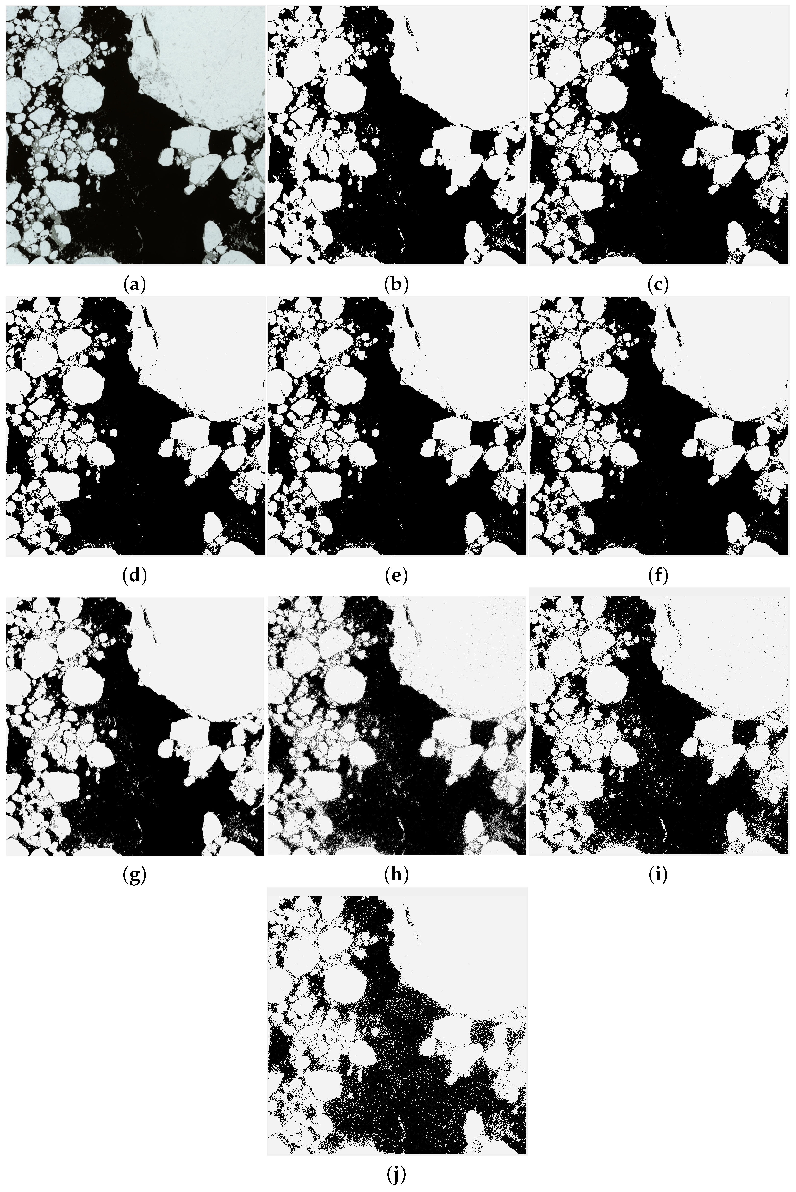
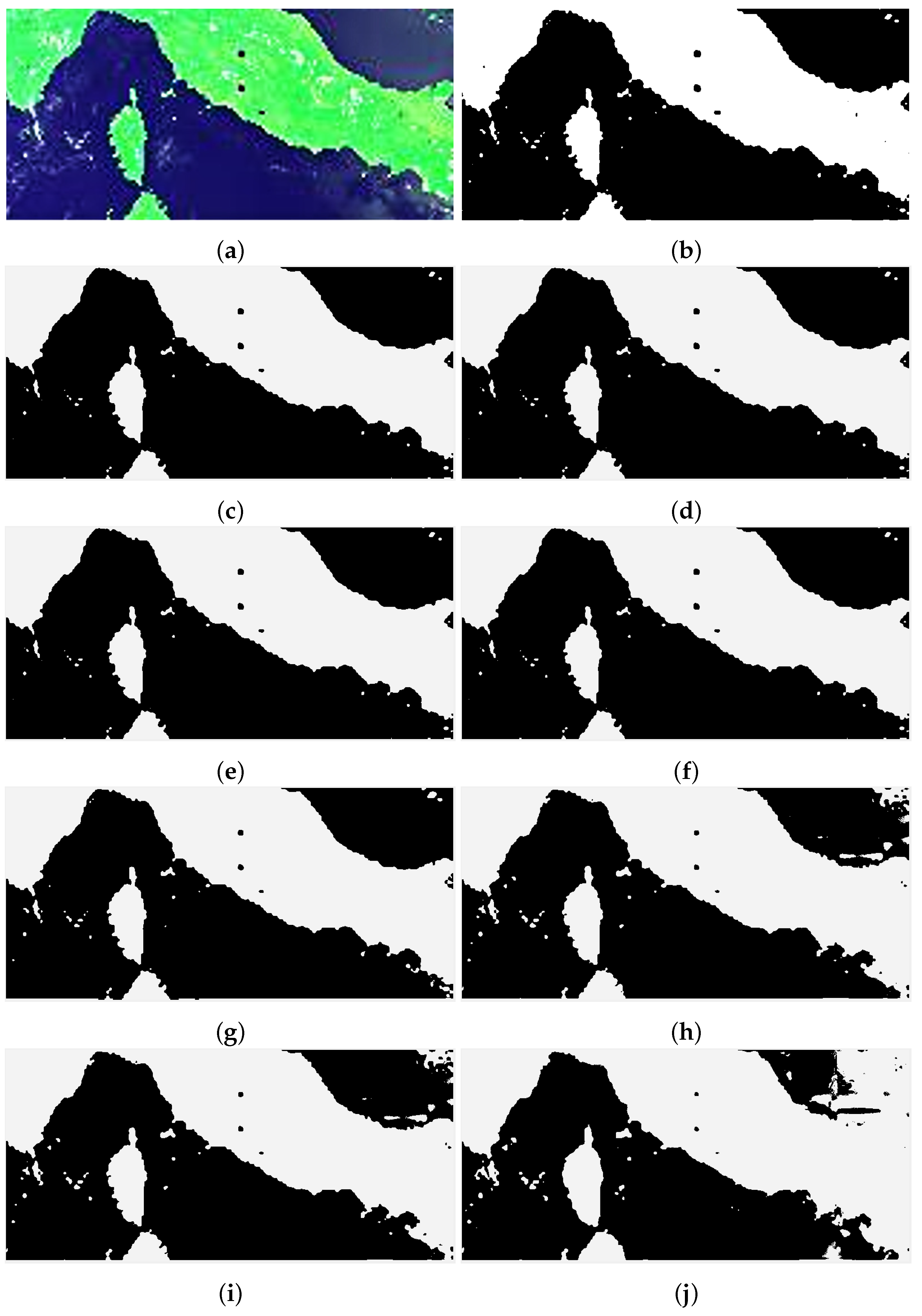
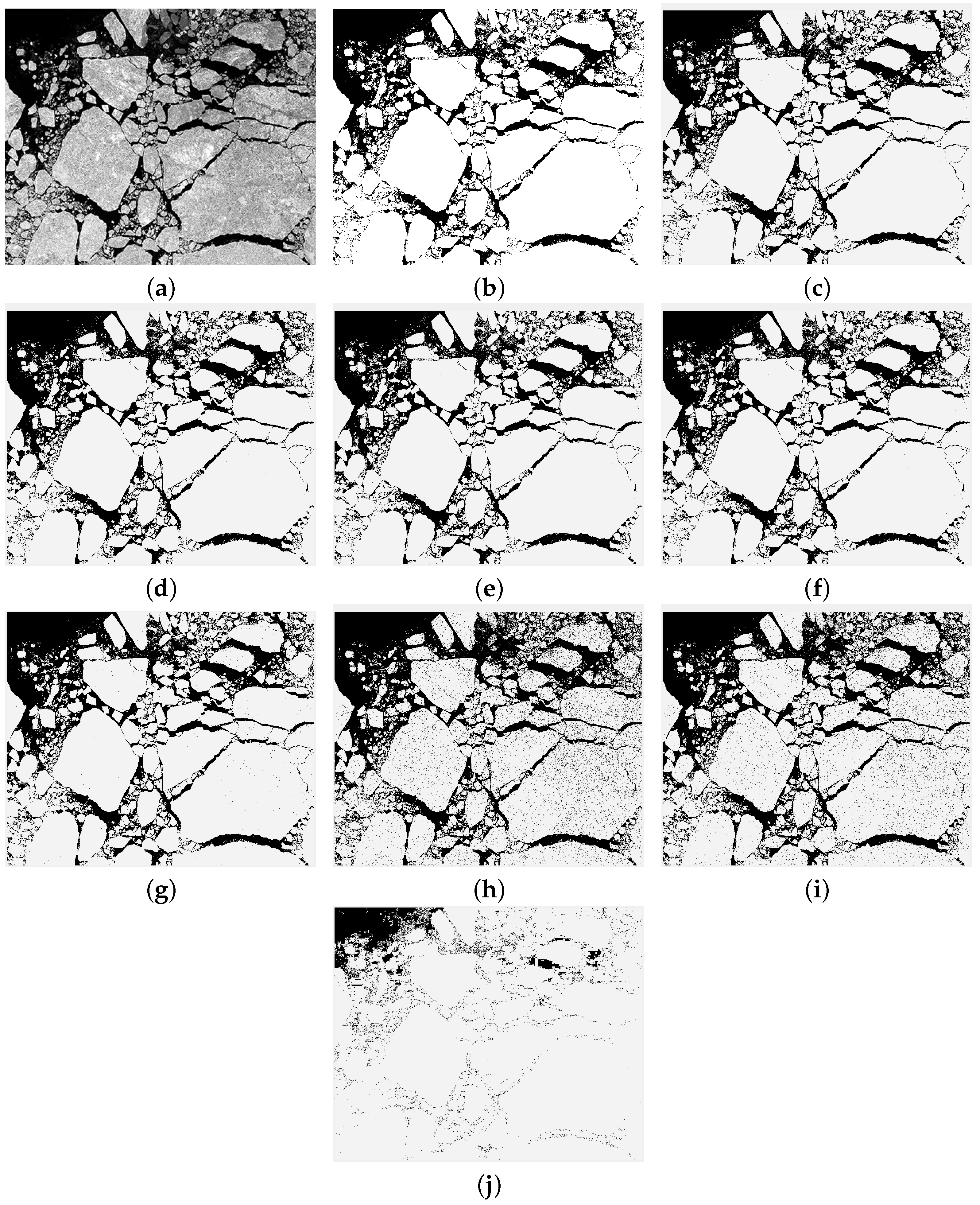
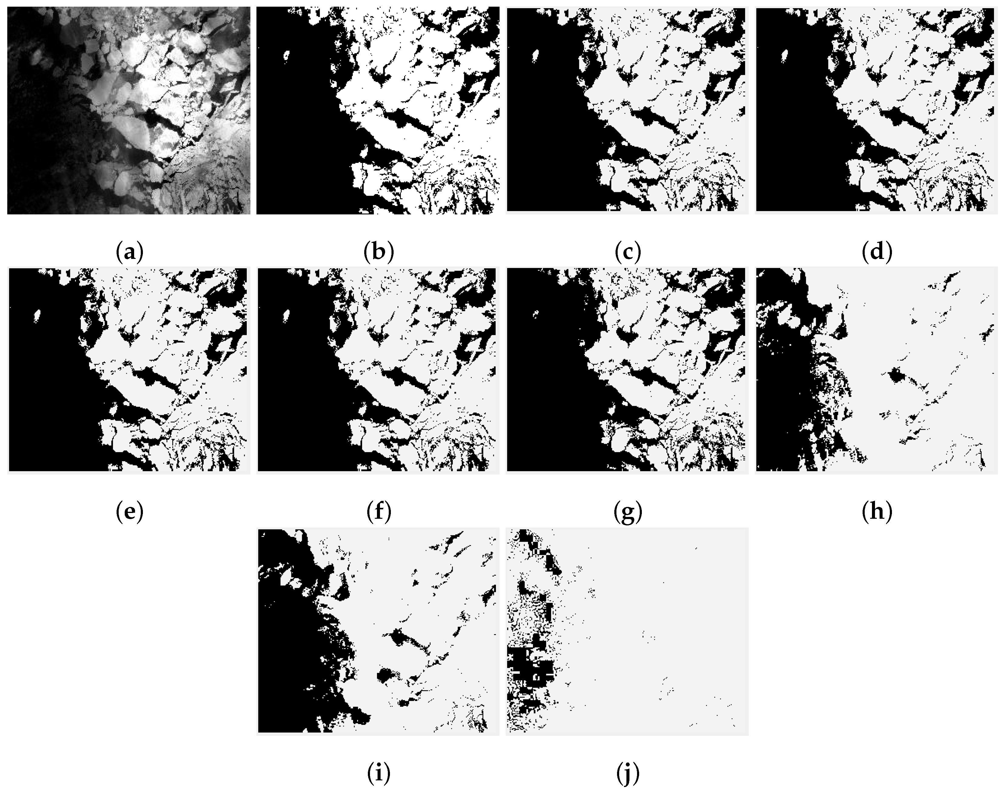
This subsection focuses on the identification of the Arctic sea ice with the aid of EAEND model (10), MNI model (27), NRI model (28), and ETZNN model (29) in the noise-free ψ ( t ) = 0 and the random noise ψ ( t ) 5 × [ 1 , 1 ] environments, respectively. Notably, some of the initial ice in the Arctic sea ice are not formed and therefore are not included in the experiments. In addition, the image identification results are shown in Figure 3, Figure 4, Figure 5 and Figure 6 and Table 1, Table 2, Table 3 and Table 4.

4.3.1. Sentinel-2

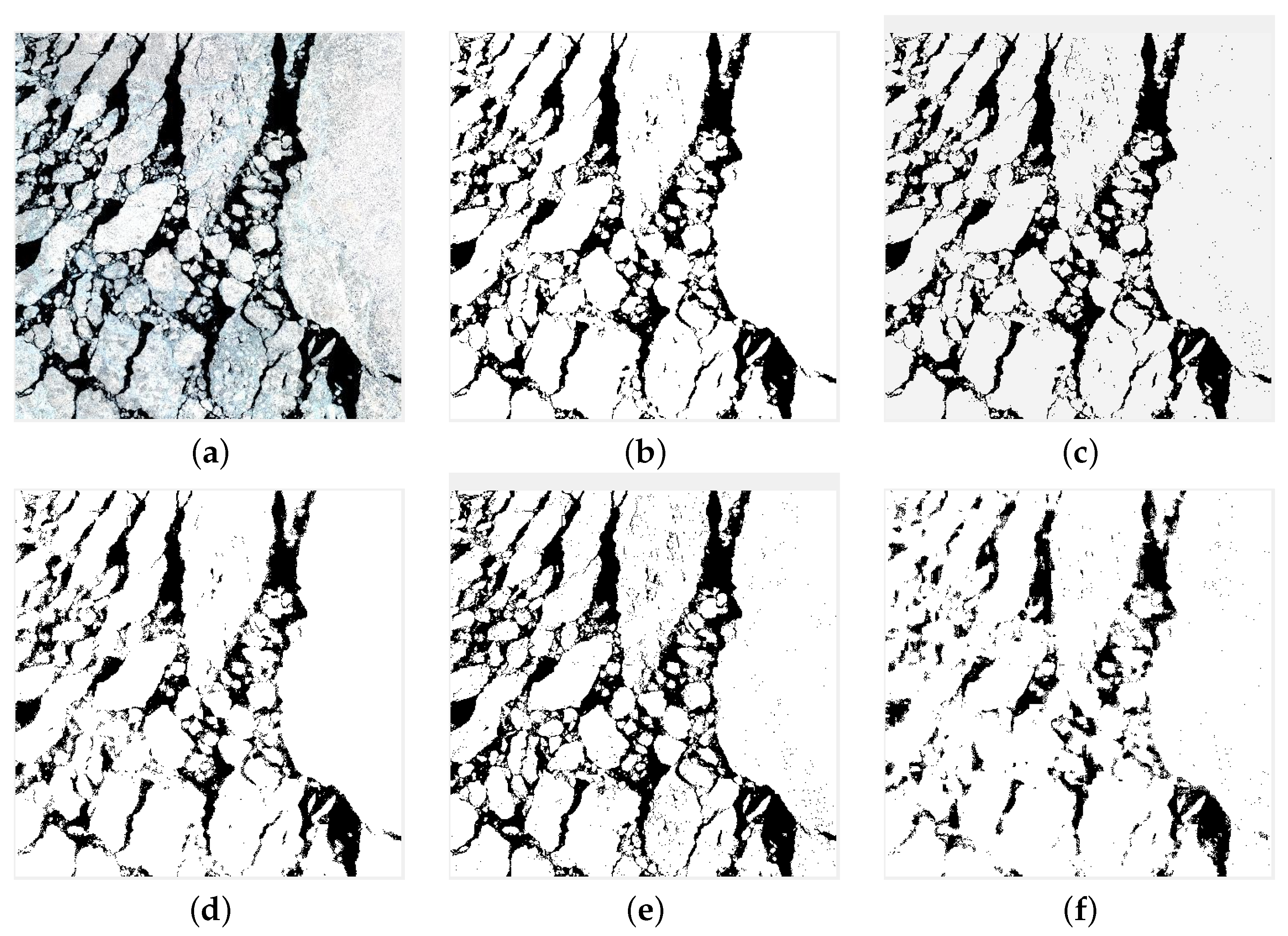
Figure 3a shows the original remote sensing image acquired from Sentinel-2, while Figure 3b is the corresponding ground-truth image. The image size is 1347 × 1347 pixels and the spatial resolution is 10 m. As seen in Figure 3c–f, all four models can consistently identify sea ice with a high degree of accuracy. In addition, from Table 1, metrics of the four models, specifically OA = 0.977508, AA = 0.979355, PP = 0.996358, and Kappa = 0.954620, are the same. Therefore, all comparison models perform well in the noise-free environment. Additionally, as shown in Table 1, all four algorithms have a high convergence accuracy for the RE. Nevertheless, as seen in Figure 3g–j, a significant difference in the performance of the three models emerges in the random noise ψ ( t ) 5 × [ 1 , 1 ] environment. Despite MNI model (27) having a noise-suppression term, it cannot maintain good identification performance, with its Kappa coefficient falling to 0.874898 and the other three indicators correspondingly decreasing. Moreover, its RE rose from 0.537140 × 10 12 in the noise-free environment to 1.189779 × 10 1 . As shown in Figure 3h, there are some misidentifications and blurred edges in the image. Although EAEND model (10) also experiences some interference, its identification accuracy can still be maintained at a Kappa value of 0.951829, and its OA, AA, and PP values are almost the same as those in the noise-free ψ ( t ) = 0 environment, demonstrating that EAEND model (10) indeed has excellent noise-resistance performance. Subsequently, NRI model (28) and ETZNN model (29) show that a large amount of noise exists in the images and the images appear blurred to varying degrees. These conditions are also reflected in the relevant numerical results in Table 1, with the RE of ETZNN model (29) reaching 10 6 . This suggests that ETZNN model (29) is not suitable for the task of sea ice identification.

4.3.2. HY-1C

In the second experiment, the Arctic sea ice image in Figure 4a is based on the observed image obtained from HY-1C with a spatial resolution of 50 m and a pixel size of 376 × 795, and Figure 4b is its ground-truth image. Both the results in Figure 4c–f and metrics in Table 2 indicate that all four models can identify sea ice images well and with high accuracy in the noise-free environment. In detail, the AA value of ETZNN model (29) is 0.993523, which is greater than that of the other three models, which shows that this method does not misidentify. In the random noise ψ ( t ) 5 × [ 1 , 1 ] environment, Figure 4g shows that EAEND model (10) still performs well, and the corresponding metrics demonstrate the stability of the model, with Kappa = 0.970668. MNI model (27) exhibits a decline in all of its indicators, which is slightly lower than that of NRI model (28). The top right-hand portion of Figure 4h–j displays misidentification, indicating that the other three models are affected by random noise, resulting in falsely identifying a portion of the ocean as sea ice, and the Kappa coefficients for the models are 0.918992, 0.923335, and 0.787680, respectively, meaning they are unable to accurately identify the Arctic sea ice.

4.3.3. ZY3-02

The third experiment was conducted based on the observation images of ZY3-02 satellite. The image has a spatial resolution of 5 m with a size of 1762 × 1450 pixels. Unlike the previous two experiments, this sea ice image contained not only large and well-defined ice blocks, but also some fragmented ice. In addition, the uneven brightness of the image caused by external interference posed a significant challenge for CEM method (1) and made it necessary to improve the performance of these four models. Firstly, as depicted in Figure 5c–f, all four models produced good results in identifying sea ice features without external noise disturbance, which was also supported by the parameters in Table 3. As depicted in Figure 5g–j, the performance of the four models shows significant variation under random noise disturbance. This highlights the increased challenge in feature identification amidst noise. Notably, EAEND model (10) exhibits superior capability in feature identification, achieving a Kappa coefficient of 0.963492. In the task of the Arctic sea ice identification, both NRI (28) and MNI (27) models produce somewhat blurred results. The distinction in feature identification quality between these models and EAEND model (10) is particularly pronounced in regions with fragmented ice. Conversely, ETZNN model (29) displays marked misidentification issues in the Arctic sea ice features, reflected in its lower OA, AA, and PP values and Kappa coefficient compared to the other three models. Furthermore, the computational performance of each model is differently impacted by random noise. ETZNN model (29), with an RE of 10 7 , struggles notably in noise suppression, aligning with the visual outcomes shown in Figure 5j.

4.3.4. HJ-2A

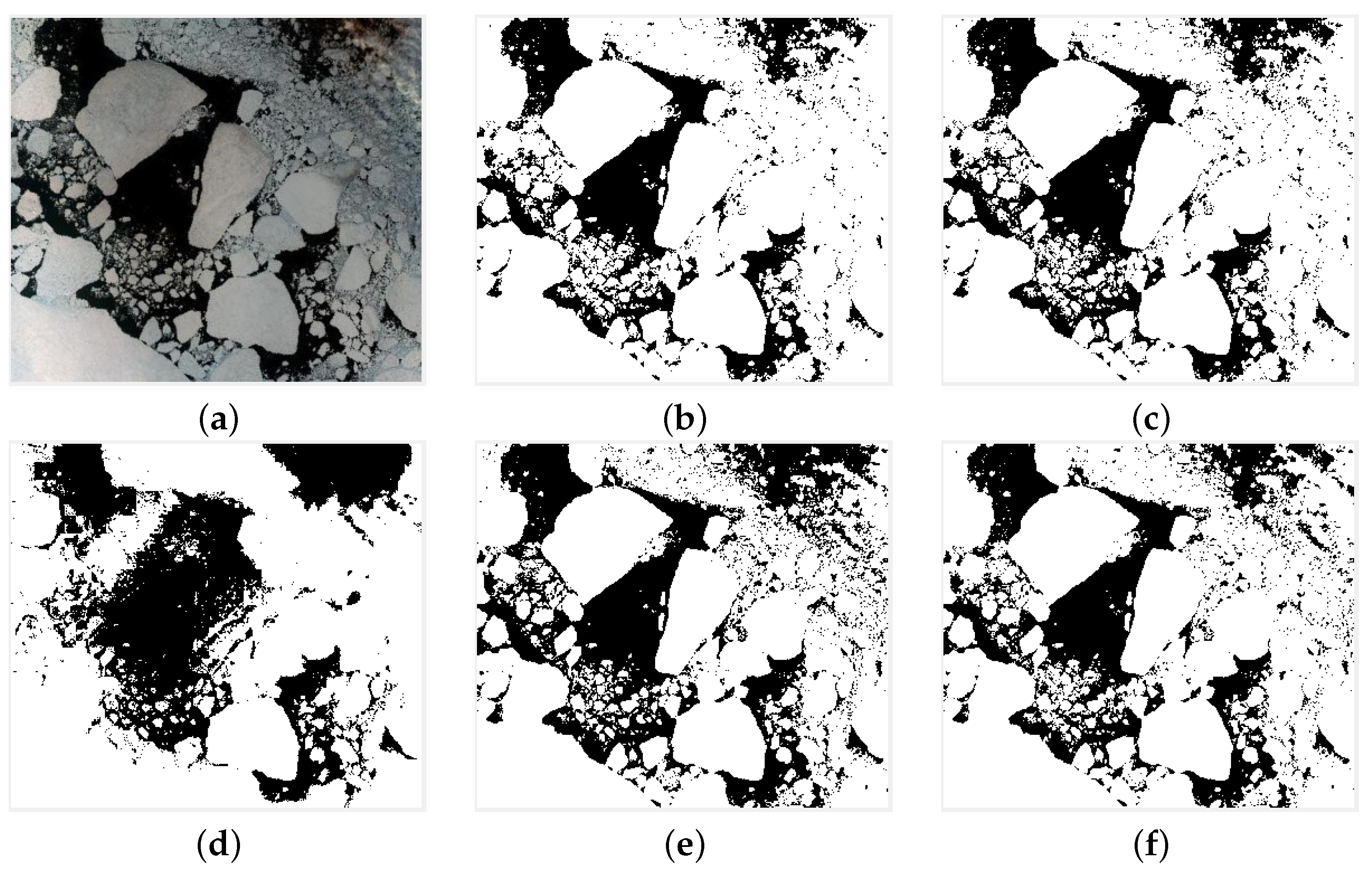
The sea ice image used in this experiment is obtained from the HJ-2A satellite, as shown in Figure 6a, with a size of 288 × 246 pixels and a spatial resolution of 16 m. Apart from some fragmented and dense sea ice, there is also fog cover in the left and upper-right parts of the image, posing significant challenges for the four models. As demonstrated in Figure 6 and Table 4, the four models perform equally well in noise-free environments, and their convergence results are impressive. Upon introducing random noise of ψ ( t ) 5 × [ 1 , 1 ] , a decline in feature identification performance is observed across all four models. EAEND model (10), in particular, fails to identify certain sea ice fragments that share similar coloration with water. This observation aligns with the numerical results and is visually corroborated in Figure 6g. Both MNI model (27) and NRI model (28) exhibit a tendency to misclassify fog and fragmented ice as sea ice, yielding Kappa coefficients of 0.455939 and 0.491205, respectively. Additionally, NRI model (28) demonstrates marginally better performance than MNI model (27) in terms of OA, AA, and PP values. The most notable underperformance is seen in ETZNN model (29), which completely fails to detect any sea ice in this experiment. Its overall performance significantly deteriorates compared to the previous three experiments.

5. Identification Experiments with Different Sensors in the Same Area

In this section, to compare the performance of the EAEND model-assisted CEM method in identifying Arctic sea ice images at different spatial resolutions, we conduct experiments on the same area using different sensors for Arctic sea ice identification. To further validate the effectiveness of the identification method, we compare the identification performance of EAEND model (10) with other traditional classification methods, which are the support vector machine (SVM) method, Otsu thresholding method, and Mahalanobis distance (MD) method.

5.1. ZY3-02 TMS

Figure 7a is sourced from the TMS sensor on the ZY3-02 satellite, with a resolution of 5 m and a size of 429 × 429 pixels. Due to the high spatial resolution, each pixel represents a smaller ground area, allowing for the capture of finer surface features. As shown in Figure 7c and Table 5, the results identified by EAEND model (10) demonstrate high values in OA, PA, and AA values and Kappa coefficient, but there are still some minor noise points on the right side. Even in smaller ice floes and broken ice areas, details are well-preserved, indicating that EAEND model (10) maintains details when processing high-resolution data. Figure 7d demonstrates that the SVM method effectively identifies the Arctic sea ice. Notably, the identification accuracy on the right side of the image surpasses that of EAEND model (10). However, the SVM method encounters difficulties in accurately segmenting fragmented ice on the left side, leading to blurred boundaries in the identified sea ice. The results using the Otsu thresholding method, as observed in the image, are marred by increased noise. This suggests that the identification process of this method is susceptible to noise interference. Figure 7f reveals the performance of the MD method in identifying the Arctic sea ice. Here, not only are the ice edges blurred to varying extents, but there is also notable misidentification. Non-ice regions with spectral similarities are incorrectly identified as sea ice, resulting in an overall unstable identification performance.

5.2. HJ-2A CCD3

As for Figure 8, the remote sensing image originates from the CCD3 sensor on the HJ-2A satellite, with a spatial resolution of 16.5 m and dimensions of 325 × 367 pixels. Compared to the TMS sensor, the CCD3 sensor has a lower spatial resolution, but the images produced are smoother with less noise and local variation, facilitating the identification of the overall Arctic sea ice imagery. During this period, the sea ice is in its melting phase, leading to the presence of numerous thin and fragmented ice pieces in the image, which increases the complexity of identification. Overall, EAEND model (10) and the MD method outperform in terms of identification results, while the Otsu thresholding method lags slightly behind. As indicated in Table 6, EAEND model (10) achieves an identification accuracy of 0.948641, excelling in other metrics as well compared to the competing methods. The SVM method, on the other hand, exhibits the weakest performance, particularly notable for its substantial under-detection in the central area of Figure 8d, where the Kappa coefficient is only 0.529627, and the OA, AA, PP have the lowest values. This underperformance implies that the SVM method is susceptible to disruption during the identification process, leading to compromised stability.

6. Discussion

In this section, we discuss and analyze the experimental results from three perspectives: the spatial resolution of sensors, the inherent characteristics of the images, and the identification methods.

6.1. Resolution of Sensors

It can be seen from the experimental results of six groups that the proposed EAEND model (10) can work effectively under different spatial resolutions, and can adapt to the change in observation scale well. In several groups of experiments from Section 4.3, optical remote sensing images of the Arctic sea ice with spatial resolutions of 10 m, 50 m, 5 m, and 16 m are selected as experimental materials. From the perspective of spatial resolution, several identification methods used for comparison (e.g., MNI model (27), NRI model (28), ETZNN model (29), SVM, Otsu thresholding, and MD) have better identification effects under different spatial resolutions. Therefore, the spatial resolution has little influence on several algorithms, indicating that several identification algorithms are universal. Further, when sensors with a spatial resolution of 16.5 m and 5 m, respectively, are used to observe the Arctic sea ice in the same region, more image details are presented with a spatial resolution of 5 m. However, this may also lead to “overfitting” in classification, that is, the identification algorithm may pay too much attention to noise or unimportant details in the image, increasing the difficulty of identification. However, the image with a spatial resolution of 16.5 m shows less feature details, and some thin and broken sea ice may fuse with the surrounding environment in the pixel, which makes it difficult for the classification algorithm to accurately distinguish these features, and it is therefore prone to the phenomenon of missing identification, as shown in Figure 7f.

6.2. Inherent Characteristics of the Images

In Section 4.3 and Section 5, the difficulty of identifying the selected images is gradually increased to show that the proposed EAEND model (10) has advantages in segmentation performance under complex conditions such as cloud cover, noise interference, and finely broken sea ice. Specifically, in Section 4.3.1 and Section 4.3.2, the outline of sea ice is relatively clear, and only a small amount of finely broken sea ice exists, which is relatively difficult to identify. In Section 4.3.3 and Section 5, remote sensing images with a spatial resolution of 5 m are used as experimental materials. Due to the high spatial resolution, the spectral information of the images is not uniform. As shown in Figure 5j, ETZNN model (29), after being disturbed by noise, also identifies non-sea ice regions with similar spectral information to sea ice by mistake, which greatly affects the segmentation performance. In Section 4.3.4, as shown in Figure 6a, there is mist and uneven illumination in the image, which easily causes the identification model to misidentify clouds with similar spectra to sea ice as sea ice, resulting in large areas of misidentification, as shown in Figure 6h–j. In addition, because the sea ice is melting, the edges of the sea ice are irregular. Under these two interference conditions from the natural environment, the identification accuracy of the model will also be greatly affected. In the experiment in Section 5.2, the illumination of the whole image is uneven, and there is a large amount of broken ice in the upper right corner of the image, which greatly affects the segmentation performance of the algorithm.

6.3. Identification Methods

The first four groups of experiments in Section 4.3 are the comparisons among the proposed EAEND model (10), MNI model model (27), NRI model (28), and ETZNN model (29), which aim to show the identification performance of several models in noise-free and random noise environments. The experimental results reveal that although MNI model (27) exhibits some resistance to noise, its identification performance is still inferior to EAEND model (10) under random noise influence. This disparity in performance can be attributed to the different expansion methods used by the models. EAEND model (10) employs the three-step forward difference formula for discretization, while MNI model (27) utilizes the second-order Euler formula. Consequently, the EAEND model (10) achieves higher accuracy. It should be noted that high-precision identification inherently involves a certain amount of computational complexity, influenced by the complexity of the formula and the size of the image. Despite this, EAEND model (10) maintains a high level of overall identification efficiency and accuracy.
Compared with the traditional identification methods (e.g., SVM method, Otsu thresholding method, and MD method), the proposed EAEND model-assisted CEM identification method has obvious advantages. First, the core principle of the SVM method lies in finding an optimal hyperplane in the feature space that maximizes the distinction between different classes. Its effectiveness largely hinges on the appropriate selection of feature spaces. The performance of SVM can be compromised if the chosen features fail to adequately differentiate between classes, or if the complexity of the feature space impedes the hyperplane’s efficient partitioning. This limitation might account for SVM’s difficulty in accurately identifying fragmented and thin sea ice. The Otsu thresholding method fundamentally revolves around selecting a threshold that maximizes the variance between the target and background classes. However, its effectiveness diminishes in images with more than two major histogram peaks, as it may struggle to establish a distinct segmentation threshold. In the sea ice identification experiment, with only water as the background, the Otsu thresholding method demonstrates effective performance. Yet, because the Otsu thresholding method itself does not have an anti-noise function, there will still be some noise on sea ice images due to small noise interference in the recognition process. The effectiveness of the MD method is contingent upon having a precise covariance matrix, which necessitates a sufficiently large sample size for accurate estimation. Inadequate sample sizes can result in miscalculations of this matrix, impairing the accuracy of distance measurements, as demonstrated in Figure 7f. By contrast, the CEM method (1) primarily depends on the target spectrum and does not require extensive samples. The susceptibility of CEM method (1) to noise is significantly diminished, aided by EAEND model (10), bolstering its broad applicability and substantially improving recognition quality.

7. Conclusions

In this paper, a CEM method has been employed to identify the Arctic sea ice from observation datasets derived from the following satellites: Sentinel-2, HY-1C, ZY3-02, and HJ-2A. Additionally, an EAEND model has been proposed to optimize the filter coefficient and facilitate the CEM method’s identification of the Arctic sea ice. Meanwhile, the proposed EAEND model with an integration term makes up for the shortcomings of the CEM method in terms of the noise immunity, improving the stability and accuracy of the CEM method for identifying Arctic sea ice. Moreover, a Taylor numerical difference formula is utilized in the construction of the EAEND model, allowing it to reach a steady-state error of O ( σ 3 ) order. Comparative identification experiments have confirmed the feasibility, accuracy, and robustness of the CEM method with the EAEND model in identifying Arctic sea ice.

Author Contributions

Conceptualization, Y.X. and D.F.; methodology, Y.X. and H.H.; software, D.W. and H.H.; validation, D.F.; formal analysis, Y.X., D.W. and H.H.; investigation, D.F.; resources, D.W.; data curation, Y.X.; writing—original draft preparation, Y.X. and D.F.; writing—review and editing, Y.X. and H.H.; visualization, Y.X. and D.W.; supervision, D.W., D.F. and H.H.; project administration, D.F.; funding acquisition, D.F. All authors have read and agreed to the published version of the manuscript.

Funding

This research was funded in part by the National Key Research and Development Program of China under Grant 2022YFC3103101, Key Special Project for Introduced Talents Team of Southern Marine Science and Engineering Guangdong Laboratory under Contract GML2021GD0809, National Natural Science Foundation of China under Contract 42206187, Key projects of the Guangdong Education Department under Grant 2023ZDZX4009.

Data Availability Statement

Data are contained within the article.

Conflicts of Interest

The authors declare no conflict of interest.

References

  1. Zelenskaya, E. Geopolitics and Tourism in the Arctic: The Case of the National Park ‘Russian Arctic’. J. Policy Res. Tour. Leis. Events 2018, 10, 33–47. [Google Scholar] [CrossRef]
  2. Saarinen, J.; Varnajot, A. The Arctic in Tourism: Complementing and Contesting Perspectives on Tourism in the Arctic. Polar Geogr. 2019, 42, 109–124. [Google Scholar] [CrossRef]
  3. Sun, Z.; Zhang, R.; Gao, Y.; Tian, Z.; Zuo, Y. Hub Ports in Economic Shocks of the Melting Arctic. Marit. Policy Manag. 2021, 48, 917–940. [Google Scholar] [CrossRef]
  4. Liu, X.; Feng, T.; Shen, X.; Li, R. PMDRnet: A Progressive Multiscale Deformable Residual Network for Multi-Image Super-Resolution of AMSR2 Arctic Sea Ice Images. IEEE Trans. Geosci. Remote Sens. 2022, 60, 4304118. [Google Scholar] [CrossRef]
  5. Perovich, D.K.; Richter-Menge, J.A. Loss of Sea Ice in the Arctic. Annu. Rev. Mar. Sci. 2009, 1, 417–441. [Google Scholar] [CrossRef]
  6. Chang, L.; Gao, G.; Li, Y.; Zhang, Y.; Zhang, C.; Zhang, Y.; Feng, G. Variations in Water Vapor from AIRS and MODIS in Response to Arctic Sea Ice Change in December 2002–2016. IEEE Trans. Geosci. Remote Sens. 2019, 57, 7395–7405. [Google Scholar] [CrossRef]
  7. Li, F.; Wan, X.; Wang, H.; Orsolini, Y.J.; Cong, Z.; Gao, Y.; Kang, S. Arctic Sea-Ice Loss Intensifies Aerosol Transport to the Tibetan Plateau. Nat. Clim. Chang. 2020, 10, 1037–1044. [Google Scholar] [CrossRef]
  8. Noh, G.H.; Ahn, K.H. Long-Lead Predictions of Early Winter Precipitation Over South Korea Using a SST Anomaly pattern in the North Atlantic Ocean. Clim. Dyn. 2022, 58, 3455–3469. [Google Scholar] [CrossRef]
  9. Dammann, D.O.; Eicken, H.; Mahoney, A.; Meyer, F.; George, J.C. Traversing Sea Ice–Linking Surface Roughness and Ice Trafficability Through SAR Polarimetry and Interferometry. IEEE J. Sel. Top. Appl. Earth Observ. 2017, 11, 416–433. [Google Scholar] [CrossRef]
  10. Li, H.; Pan, D.; Wang, D.; Gong, F.; Bai, Y.; He, X.; Hao, Z.; Ke, C. The Impact of Summer Arctic Cyclones on Chlorophyll–A Concentration and Sea Surface Temperature in the Kara Sea. IEEE J. Sel. Top. Appl. Earth Observ. 2019, 12, 1396–1408. [Google Scholar] [CrossRef]
  11. Larson, E. Turning the World Upside Down. Nature 2011, 480, 29–31. [Google Scholar] [CrossRef]
  12. Cavalieri, D.J.; Gloersen, P.; Wilheit, T.T. Aircraft and Satellite Passive Microwave Observations of the Bering Sea Ice Cover During MIZEX West. IEEE Trans. Geosci. Remote Sens. 1986, 368–377. [Google Scholar] [CrossRef]
  13. Mikhalevsky, P.N.; Gavrilov, A.N.; Baggeroer, A.B. The Transarctic Acoustic Propagation Eexperiment and Climate Monitoring in the Arctic. IEEE J. Ocean Eng. 1999, 24, 183–201. [Google Scholar] [CrossRef]
  14. Crocker, R.I.; Maslanik, J.A.; Adler, J.J.; Palo, S.E.; Herzfeld, U.C.; Emery, W.J. A Sensor Package for Ice Surface Observations Using Small Unmanned Aircraft Systems. IEEE Trans. Geosci. Remote Sens. 2011, 50, 1033–1047. [Google Scholar] [CrossRef]
  15. Nghiem, S.V.; Clemete-Colon, P. Arctic Sea Ice Mapping with Satellite Radars. IEEE Trans. Aerosp. Electron. Syst. 2009, 24, 41–44. [Google Scholar] [CrossRef]
  16. Gollin, N.; Giez, J.; Martone, M.; Rizzoli, P.; Scheiber, R.; Krieger, G. Dynamic Predictive Quantization for Staggered SAR: Experiments with Real Data. IEEE Trans. Geosci. Remote Sens. Lett. 2023, 20, 4000605. [Google Scholar] [CrossRef]
  17. Du, Z.; Li, X.; Miao, J.; Huang, Y.; Shen, H.; Zhang, L. Concatenated Deep Learning Framework for Multi-task Change Detection of Optical and SAR Images. IEEE J. Sel. Top. Appl. Earth Observ. 2023; early access. [Google Scholar] [CrossRef]
  18. Pacifici, F.; Del Frate, F.; Solimini, C.; Emery, W.J. An Innovative Neural-Net Method to Detect Temporal Changes in High-Resolution Optical Satellite Imagery. IEEE Trans. Geosci. Remote Sens. 2007, 45, 2940–2952. [Google Scholar] [CrossRef]
  19. Osadchiev, A.; Sedakov, R. Spreading Dynamics of Small River Plumes Off the Northeastern Coast of the Black Sea Observed by Landsat 8 and Sentinel-2. Remote Sens. Environ. 2019, 221, 522–533. [Google Scholar] [CrossRef]
  20. Ye, X.; Liu, J.; Lin, M.; Ding, J.; Zou, B.; Song, Q. Global Ocean Chlorophyll-a Concentrations Derived from COCTS Onboard the HY-1C Satellite and Their Preliminary Evaluation. IEEE Trans. Geosci. Remote Sens. 2020, 59, 9914–9926. [Google Scholar] [CrossRef]
  21. Wang, Y.; Dou, Y.; Guo, J.; Yang, Z.; Yang, B.; Sun, Y.; Liu, W. Feasibility Study for an Ice-Based Image Monitoring System for Polar Regions Using Improved Visual Enhancement Algorithms. IEEE J. Sel. Top. Appl. Earth Observ. 2022, 15, 3788–3799. [Google Scholar] [CrossRef]
  22. Haverkamp, D.; Soh, L.K.; Tsatsoulis, C. A Dynamic Local Thresholding Technique for Sea Ice Classification. In Proceedings of the IGARSS’93-IEEE International Geoscience and Remote Sensing Symposium, Tokyo, Japan, 18–21 August 1993; IEEE: Piscataway, NJ, USA, 1993; pp. 638–640. [Google Scholar]
  23. Komarov, A.S.; Buehner, M. Adaptive Probability Thresholding in Automated Ice and Open Water Detection from RADARSAT-2 Images. IEEE Geosci. Remote Sens. Lett. 2018, 15, 552–556. [Google Scholar] [CrossRef]
  24. Lindsay, R.W.; Percival, D.B.; Rothrock, D.A. The Discrete Wavelet Transform and the Scale Analysis of the Surface Properties of Sea Ice. IEEE Trans. Geosci. Remote Sens. 1996, 4, 771–787. [Google Scholar] [CrossRef]
  25. Li, X.M.; Sun, Y.; Zhang, Q. Extraction of Sea Ice Cover By Sentinel-1 SAR Based on Support Vector Machine with Unsupervised Generation of Training Data. IEEE Trans. Geosci. Remote Sens. 2020, 59, 3040–3053. [Google Scholar] [CrossRef]
  26. Xie, H.; He, S.; Cheng, X. A Convolution Neural Network-based Method for Sea Ice Remote Sensing Using GNSS-R Data. In Proceedings of the 2022 4th International Conference on Communications, Information System and Computer Engineering (CISCE), Shenzhen, China, 27–29 May 2022; pp. 284–289. [Google Scholar]
  27. Jiang, M.; Xu, L.; Clausi, D.A. Sea Ice–Classification of RADARSAT-2 Imagery Based on Residual Neural Networks (ResNet) with Regional Pooling. Remote Sens. 2022, 14, 3025. [Google Scholar] [CrossRef]
  28. Zhong, H.F.; Sun, H.M.; Jia, R.S.; Zhang, Q. FR-GAN: A Self-Supervised Learning Method for Super-Resolution Reconstruction of Optical Remote Sensing Images. J. Appl. Remote Sens. 2022, 16, 026509. [Google Scholar] [CrossRef]
  29. Harsanyi, J.C. Detection and Classification of Subpixel Spectral Signatures in Hyperspectral Image Sequences; Department of Electrical Engineering University of Maryland: Baltimore County, ML, USA, 1993. [Google Scholar]
  30. Ma, K.Y.; Chang, C.I. Kernel-Based Constrained Energy Minimization for Hyperspectral Mixed Pixel Classification. IEEE Trans. Geosci. Remote Sens. 2021, 60, 5510723. [Google Scholar] [CrossRef]
  31. Zhong, Y.; Liao, S.; Yu, G.; Fu, D.; Huang, H. Harbor Aquaculture Area Extraction Aided with an Integration-Enhanced Gradient Descent Algorithm. Remote Sens. 2021, 13, 4554. [Google Scholar] [CrossRef]
  32. Chowdhury, S.; Chao, D.K.; Shipman, T.C.; Wulder, M.A. Utilization of Landsat Data to Quantify Land-Use and Land-Cover Changes Related to Oil and Gas Activities in West-Central Alberta from 2005 to 2013. GISci. Remote Sens. 2017, 54, 700–720. [Google Scholar] [CrossRef]
  33. Brown, J.C.; Jepson, W.E.; Kastens, J.H.; Wardlow, B.D.; Lomas, J.M.; Price, K.P. Multitemporal, Moderate-Spatial-Resolution Remote Sensing of Modern Agricultural Production and Land Modification in the Brazilian Amazon. GISci. Remote Sens. 2007, 44, 117–148. [Google Scholar] [CrossRef]
  34. Maiti, S.; Bhattacharya, A.K. A Three-Unit-Based Approach in Coastal-Change Studies Using Landsat Images. Int. J. Remote Sens. 2011, 32, 209–229. [Google Scholar] [CrossRef]
  35. Chang, C.I. Constrained Energy Minimization Anomaly Detection for Hyperspectral Imagery Via Dummy Variable Trick. IEEE Trans. Geosci. Remote Sens. 2021, 60, 5517119. [Google Scholar] [CrossRef]
  36. Xi, Y.; Ji, L.; Yang, W.; Geng, X.; Zhao, Y. Multitarget Detection Algorithms for Multitemporal Remote Sensing Data. IEEE Trans. Geosci. Remote Sens. 2020, 60, 5400115. [Google Scholar] [CrossRef]
  37. Zhu, X.; Li, S.; Zhang, X.; Li, H.; Kot, A.C. Detection of Spoofing Medium Contours for Face Anti–Spoofing. IEEE Trans. Circuits Syst. Video Technol. 2019, 31, 2039–2045. [Google Scholar] [CrossRef]
  38. Zhang, Y.; Ma, W.; Cai, B. From Zhang Neural Network to Newton Iteration for Matrix Inversion. IEEE Trans. Circuits Syst. I Regul. Pap. 2008, 56, 1405–1415. [Google Scholar] [CrossRef]
  39. Jin, L.; Li, S.; Liao, B.; Zhang, Z. Zeroing Neural Networks: A Survey. Neurocomputing 2017, 267, 597–604. [Google Scholar] [CrossRef]
  40. Chen, D.; Zhang, Y. Robust Zeroing Neural-Dynamics and Its Time-Varying Disturbances Suppression Model Applied to Mobile Robot Manipulators. IEEE Trans. Neural Netw. Learn. Syst. 2017, 29, 4385–4397. [Google Scholar] [CrossRef] [PubMed]
  41. Xiong, Y.; Wang, D.; Fu, D.; Wang, Y. Discrete-Time Noise-Suppression Neural Dynamics for Optical Remote Sensing Image Extraction. IEEE Access 2023, 11, 92111–92119. [Google Scholar] [CrossRef]
  42. Jin, L.; Yan, J.; Du, X.; Xiao, X.; Fu, D. RNN for Solving Time-Variant Generalized Sylvester Equation with Applications to Robots and Acoustic Source Localization. IEEE Trans. Ind. Inform. 2020, 16, 6359–6369. [Google Scholar] [CrossRef]
  43. Zhang, Y.; Xiao, Z.; Guo, D.; Mao, M.; Yin, Y. Singularity Tracking Control of A Class of Chaotic Systems Using Zhang Dynamics. IET Control Theory Appl. 2015, 9, 871–881. [Google Scholar] [CrossRef]
  44. Zhang, Y.; Yan, X.; Liao, B.; Zhang, Y.; Ding, Y. Z-Type Control of Populations for Lotka–Volterra Model with Exponential Convergence. Math. Biosci. 2016, 272, 15–23. [Google Scholar] [CrossRef]
  45. Qi, Y.; Jin, L.; Wang, Y.; Xiao, L.; Zhang, J. Complex-Valued Discrete-Time Neural Dynamics for Perturbed Time-Dependent Complex Quadratic Programming with Applications. IEEE Trans. Neural Netw. Learn. Syst. 2019, 31, 3555–3569. [Google Scholar] [CrossRef] [PubMed]
  46. Liu, M.; Zhang, X.; Shang, M. Computational Neural Dynamics Model for Time-Variant Constrained Nonlinear Optimization Applied to Winner-Take-All Operation. IEEE Trans. Ind. Inform. 2021, 18, 5936–5948. [Google Scholar] [CrossRef]
  47. Jin, L.; Liufu, Y.; Lu, H.; Zhang, Z. Saturation-Allowed Neural Dynamics Applied to Perturbed Time-Dependent System of Linear Equations and Robots. IEEE Trans. Ind. Electron. 2021, 68, 9844–9854. [Google Scholar] [CrossRef]
  48. Jin, L.; Zhang, Y.; Qiu, B. Neural Network-Based Discrete-Time Z-Type Model of High Accuracy in Noisy Environments for Solving Dynamic System of Linear Equations. Neural Comput. Appl. 2018, 29, 1217–1232. [Google Scholar] [CrossRef]
  49. Liufu, Y.; Jin, L.; Xu, J.; Xiao, X.; Fu, D. Reformative Noise-Immune Neural Network for Equality-Constrained Optimization Applied to Image Target Detection. IEEE Trans. Emerg. Top. Comput. 2021, 10, 973–984. [Google Scholar] [CrossRef]
  50. Huang, H.; Fu, D.; Xiao, X.; Ning, Y.; Wang, H.; Jin, L.; Liao, S. Modified Newton Integration Neural Algorithm for Dynamic Complex-Valued Matrix Pseudoinversion Applied to Mobile Object Localization. IEEE Trans. Ind. Inform. 2020, 17, 2432–2442. [Google Scholar] [CrossRef]
  51. Jin, L.; Li, S.; Hu, B.; Liu, M.; Yu, J. A Noise-Suppressing Neural Algorithm for Solving The Time-Varying System of Linear Equations: A Control-Based Approach. IEEE Trans. Ind. Inform. 2018, 15, 236–246. [Google Scholar] [CrossRef]
  52. Fu, D.; Huang, H.; Xiao, X.; Xia, L.; Jin, L. A Generalized Complex-Valued Constrained Energy Minimization Scheme for The Arctic Sea Ice Extraction Aided with Neural Algorithm. IEEE Trans. Geosci. Remote Sens. 2021, 60, 4303017. [Google Scholar] [CrossRef]
  53. Li, W.; Swetits, J. A Newton Method for Convex Regression, Data Smoothing, and Quadratic Programming with Bounded Constraints. SIAM J. Optim. 1993, 3, 466–488. [Google Scholar] [CrossRef]
  54. Lu, Y.; Zhang, B.; Perrie, W. Arctic Sea Ice and Open Water Classification from Spaceborne Fully Polarimetric Synthetic Aperture Radar. IEEE Trans. Geosci. Remote Sens. 2023, 61, 4203713. [Google Scholar] [CrossRef]
  55. Hwang, B.; Wang, Y. Multi-Scale Satellite Observations of Arctic Sea Ice: New Insight Into The Life Cycle of The Floe Size Distribution. Philos. Trans. R. Soc. A 2022, 380, 20210259. [Google Scholar] [CrossRef] [PubMed]
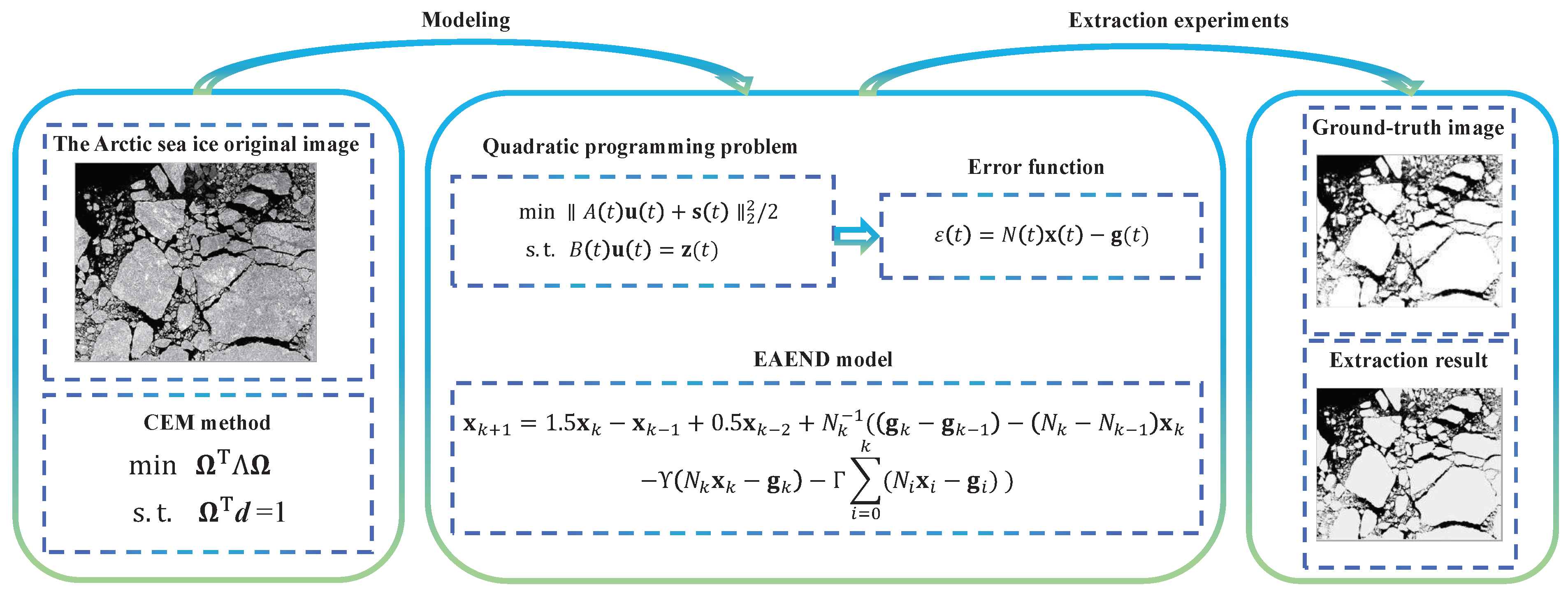
Figure 1. Technical route of Arctic sea ice identification.
Remotesensing 15 05555 g001
Figure 2. Observation area.
Remotesensing 15 05555 g002
Figure 3. Identification results of four algorithm-assisted CEM method (1) for the Arctic sea ice from Sentinel-2. (a) Original image. (b) Ground truth. (cf) Identification results of EAEND model (10), MNI model (27), NRI model (28), and ETZNN model (29) in the noise-free ψ ( t ) = 0 environment. (gj) Identification results of EAEND model (10), MNI model (27), NRI model (28), and ETZNN model (29) in the random noise ψ ( t ) 5 × [ 1 , 1 ] environment.
Remotesensing 15 05555 g003
Figure 4. Identification results of four algorithm-assisted CEM method (1) for the Arctic sea ice from HY-1C. (a) Original image. (b) Ground truth. (cf) Identification results of EAEND model (10), MNI model (27), NRI model (28), and ETZNN model (29) in the noise-free ψ ( t ) = 0 environment. (gj) Identification results of EAEND model (10), MNI model (27), NRI model (28), and ETZNN model (29) in the random noise ψ ( t ) 5 × [ 1 , 1 ] environment.
Remotesensing 15 05555 g004
Figure 5. Identification results of four algorithm-assisted CEM method (1) for the Arctic sea ice from ZY3-02. (a) Original image. (b) Ground truth. (cf) Identification results of EAEND model (10), MNI model (27), NRI model (28), and ETZNN model (29) in the noise-free ψ ( t ) = 0 environment. (gj) Identification results of EAEND model (10), MNI model (27), NRI model (28), and ETZNN model (29) in the random noise ψ ( t ) 5 × [ 1 , 1 ] environment.
Remotesensing 15 05555 g005
Figure 6. Identification results of four algorithm-assisted CEM method (1) for the Arctic sea ice from HJ-2A. (a) Original image. (b) Ground truth. (cf) Identification results of EAEND model (10), MNI model (27), NRI model (28), and ETZNN model (29) in the noise-free ψ ( t ) = 0 environment. (gj) Identification results of EAEND model (10), MNI model (27), NRI model (28), and ETZNN model (29) in the random noise ψ ( t ) 5 × [ 1 , 1 ] environment.
Remotesensing 15 05555 g006
Figure 7. Identification results of four algorithm-assisted CEM method (1) for the Arctic sea ice from ZY3-02 TMS. (a) Original image. (b) Ground truth. (cf) Identification results of EAEND model (10), SVM method, Otsu thresholding method, MD method.
Remotesensing 15 05555 g007
Figure 8. Identification results of four algorithm-assisted CEM method (1) for the Arctic sea ice from HJ-2A CCD3. (a) Original image. (b) Ground truth. (cf) Identification results of EAEND model (10), SVM method, Otsu thresholding method, MD method.
Remotesensing 15 05555 g008
Table 1. Identification metrics and results of four algorithm-assisted CEM method (1) for the Arctic sea ice from Sentinel-2.
Performance IndexNoise-Free ψ ( t ) = 0 Random Noise ψ ( t ) 5 × [ 1 , 1 ]
EAENDMNINRIETZNNEAENDMNINRIETZNN
RE 3 . 705857 × 10 12 1 . 537140 × 10 12 1.097830 × 10 12 2.960869 × 10 7 1 . 185912 × 10 1 1.189779 × 10 1 9.219882 × 10 0 1.438138 × 10 6
OA0.9775080.9775080.9775080.9775080.9762170.9384270.9441740.919061
AA0.9793550.9793550.9793550.9793550.9761050.9362660.9426940.911631
PP0.9963580.9963580.9963580.9963580.9801480.9355520.9447200.888814
Kappa0.9546200.9546200.9546200.9546200.9518290.8748980.8867120.833880
Table 2. Identification metrics and results of four algorithm-assisted CEM method (1) for the Arctic sea ice from HY-1C.
Performance IndexNoise-Free ψ ( t ) = 0 Random Noise ψ ( t ) 5 × [ 1 , 1 ]
EAENDMNINRIETZNNEAENDMNINRIETZNN
RE 2.964768 × 10 13 1.485357 × 10 13 3.552714 × 10 14 1.053860 × 10 1 1.122136 × 10 1 1.086109 × 10 1 8.891720 × 10 0 8.775299 × 10 5
OA0.9935400.9935400.9935400.9935300.9858490.9605010.9626520.893607
AA0.9935170.9935170.9935170.9935230.9881900.9671370.9689260.911480
PP0.9904380.9904380.9904380.9903310.9659480.9099320.9144170.789504
Kappa0.9865380.9865380.9865380.9865170.9706680.9189920.9233350.787680
Table 3. Identification metrics and results of four algorithm-assisted CEM method (1) for the Arctic sea ice from ZY3-02.
Performance IndexNoise-Free ψ ( t ) = 0 Random Noise ψ ( t ) 5 × [ 1 , 1 ]
EAENDMNINRIETZNNEAENDMNINRIETZNN
RE 2.273738 × 10 13 5.684385 × 10 14 5 . 684353 × 10 14 1.136990 × 10 13 5 . 659684 × 10 0 1.044903 × 10 1 7.025637 × 10 0 2.006999 × 10 7
OA0.9873690.9873690.9873690.9873690.9860700.9464870.9547050.805042
AA0.9913060.9913060.9913060.9913060.9740540.9003260.9156330.636869
PP0.9998560.9998560.9998560.9998560.9813150.9318370.9416940.789579
Kappa0.9678890.9678890.9678890.9678890.9639420.8545750.8781690.355451
Table 4. Identification metrics and results of four algorithm-assisted CEM method (1) for the Arctic sea ice from HJ-2A.
Performance IndexNoise-Free ψ ( t ) = 0 Random Noise ψ ( t ) 5 × [ 1 , 1 ]
EAENDMNINRIETZNNEAENDMNINRIETZNN
RE 1.136869 × 10 13 2.842171 × 10 14 2.842171 × 10 14 2.960869 × 10 7 5 . 659684 × 10 0 1.044903 × 10 1 7.025637 × 10 0 2.006999 × 10 7
OA0.9830060.9830060.9830060.9830060.9647550.7191590.7379880.543572
AA0.9840470.9840470.9840470.9840470.9622960.7363580.7540350.571525
PP0.9649150.9649150.9649150.9649151.0000000.6246560.6407810.505928
Kappa0.9659420.9659420.9659420.9659420.9288810.4559390.4912050.134977
Table 5. Identification metrics and results of four methods for the Arctic sea ice from ZY3-02 TMS.
MethodEAENDSVMOtsu ThresholdingMD
Metrics
OA0.9825330.9743690.9659960.928233
AA0.9886340.9322120.9790350.979034
PP0.9996290.9693621.0000000.922038
Kappa0.9449200.9118250.8962570.730540
Table 6. Identification metrics and results of four methods for the Arctic sea ice from HJ-2A CCD3.
MethodEAENDSVMOtsu ThresholdingMD
Metrics
OA0.9809680.8093220.9222210.965818
AA0.9875460.7977670.9491040.976625
PP1.0000000.9693621.0000000.999060
Kappa0.9486410.5296270.8063260.909534
Disclaimer/Publisher’s Note: The statements, opinions and data contained in all publications are solely those of the individual author(s) and contributor(s) and not of MDPI and/or the editor(s). MDPI and/or the editor(s) disclaim responsibility for any injury to people or property resulting from any ideas, methods, instructions or products referred to in the content.