Motorcycle Detection and Collision Warning Using Monocular Images from a Vehicle

Abstract

Motorcycle detection and collision warning are essential features in advanced driver assistance systems (ADAS) to ensure road safety, especially in emergency situations. However, detecting motorcycles from videos captured from a car is challenging due to the varying shapes and appearances of motorcycles. In this paper, we propose an integrated and innovative remote sensing and artificial intelligence (AI) methodology for motorcycle detection and distance estimation based on visual data from a single camera installed in the back of a vehicle. Firstly, MD-TinyYOLOv4 is used for detecting motorcycles, refining the neural network through SPP (spatial pyramid pooling) feature extraction, Mish activation function, data augmentation techniques, and optimized anchor boxes for training. The proposed algorithm outperforms eight existing YOLO versions, achieving a precision of 81% at a speed of 240 fps. Secondly, a refined disparity map of each motorcycle’s bounding box is estimated by training a Monodepth2 with a bilateral filter for distance estimation. The proposed fusion model (motorcycle’s detection and distance from vehicle) is evaluated with depth stereo camera measurements, and the results show that 89% of warning scenes are correctly detected, with an alarm notification time of 0.022 s for each image. Outcomes indicate that the proposed integrated methodology provides an effective solution for ADAS, with promising results for real-world applications, and can be suitable for running on mobility services or embedded computing boards instead of the super expensive and powerful systems used in some high-tech unmanned vehicles.

1. Introduction

According to the National Highway Traffic Safety Administration (NHTSA), motorcycle accidents were responsible for approximately 14% of all accident fatalities in the last decade. Numerous studies have been conducted in an attempt to reduce the number of accidents in transportation systems, with a focus on designing advanced driver assistance systems (ADAS) that can detect danger and provide warnings to prevent dangerous car accidents using a variety of sensors [1,2,3,4]. Although active sensors are effective for safe driving [5,6], they remain expensive, often costing as much as the vehicle itself [1], and can be easily damaged in small collisions. In contrast, cameras have gained popularity due to their simpler image processing techniques, practicality, and lower cost for use in ADAS applications [7].

However, motorcycles remain one of the most challenging objects on the road to detect, as they have different shapes and sizes depending on the manufacturer, and their appearance can vary depending on the country of use. For example, a report released by the Tehran Police revealed that a significant number of motorcycle accidents on Tehran’s streets involve motorcycles with black windshields, as shown in Figure 1. Although this type of windshield provides motorcycle drivers with better protection against the wind, debris, bugs, and extreme temperatures, riding with it may create difficulties in steering or decrease visibility, increasing the likelihood of accidents. Furthermore, the difference in appearance can cause problems for existing motorcycle detection algorithms, leading to inaccurate bounding box estimation and false detection results. Therefore, there is a need to develop a methodology that can accurately detect this type of motorcycle, monitor and track its relative location, and provide appropriate data and information for drivers to promote safer driving.

Existing methods of driver warning algorithms can use either one network or a combination of two different algorithms for object detection and depth estimation. DisNet [8] is a one-network approach that combines YOLOv3 and a fully connected neural network to detect bounding boxes with distances, although it is only calculated on specific static scenes. In Dist-YOLO [9], the distance estimation task is integrated with the YOLO architecture and the heads predicting vectors are extended with appropriate information about distances. These models require an enriched dataset that has label distance information for each drawn bounding box, which is mostly obtained through LiDAR or on-site measurement data. Therefore, most recent studies have focused on detecting motorcycles with helmets [10,11,12,13] or license plates [14,15] and then calculating their distance based on the size of the detected motorcycle [16,17]. Furthermore, ADAS systems bloomed specifically in difficult and challenging situations such as motorcycle safety relying on warning systems for motorcyclists by using YOLOv4 and machine learning techniques based on dual-lens stereo cameras [18] or warning vehicle drivers using multi-camera data [19]. However, these studies could not determine the distance between the camera and the vehicles with a single camera.

In recent years, numerous studies have focused on using convolutional neural network (CNN) algorithms for road vehicle detection applications from single-camera images [15,20]. CNN models are typically classified into two types: two-stage and single-stage methods. In two-stage methods, the algorithm first identifies the proposed area of the object’s presence and then determines the class type of the identified object. Some common two-stage methods are R-CNN [21], Fast-R-CNN [22], and Faster-R-CNN [23], which are generally time-consuming for real-time object detection applications. In contrast, single-stage approaches perform object localization and classification simultaneously in one step, making them faster with respect to two-stage methods [24]. In the ADAS application, SSD (Single Shot MultiBox Detector) [25] and YOLO [26,27,28,29] are state-of-the-art single-stage algorithms for real-time helmeted and non-helmeted motorcycle detection [30]. In addition, combining YOLO and CNN techniques helps in achieving better automatic helmet detection [12], face detection [31,32], license plate recognition [33], and vehicle [34] and pedestrian detection [35] for vulnerable road user safety. Based on prior studies in detecting cars, motorcycles, and pedestrians based on the VOC2012 database [36], the YOLOv2 [26] achieved the same accuracy six and two times faster than Faster R-CNN and SSD, respectively. To increase motorcycle detection accuracy, YOLOv2 was also used for human detection as well as helmet detection [14]. However, there is evidence that due to the small size and poor quality of the motorcycle images, YOLOv3 [27] was unable to detect motorcycles in some situations [37]. Despite this, YOLOv3 is generally fast in performing vehicle detection in complex scenes based on training on the VOC dataset compared to other traditional object detection algorithms [24]. Furthermore, the refined YOLOv4 [38] achieved an average accuracy of 67% and a speed of 38 fps in car, truck, and motorcycle tracking applications. Finally, although the YOLOv5 [39] model was used for safety vehicle detection mechanisms [40], reservations exist, as it was not developed by the original author of YOLO and is less innovative than previous versions [41]. Tiny architectures for the YOLO algorithm series were proposed in order to use fewer computational resources than the full-scale YOLO series, allowing for higher-speed performance, even on mobile devices or embedded systems [42].

In addition to object detection, a variety of information, such as depth maps and distance values, can also be obtained from camera calibration and road objects by means of different methods like linear regression and the pinhole algorithm [43,44,45]. Two other basic approaches in the image depth map estimation field are SLAM (simultaneous localization and mapping) [46] and SfM (structure-from-motion) [47], which use object and scene movements to evaluate depth [48]. Although SfM regularly performs better than SLAM, SfM is not applicable in ADAS applications because information regarding the camera’s pose and movements is needed in all three directions for depth estimation [49]. Therefore, deep learning methods may solve some of these problems in depth and pose estimation. Deep learning methods in depth map estimation are broadly divided into two types: supervised [50] and unsupervised learning methods [51]. Supervised models predict depth by training them with massive amounts of corresponding ground-truth depth map data [52], the real distances from the object in the KITTI dataset to the camera [53], or with a combination of Video and RTK GNSS data [54]. Since this process is costly and training data are difficult to obtain, unsupervised or self-supervised networks have been used for depth estimation from a single image [51,55]. Compared to conventional stereo-based methods, self-supervised depth estimators provide widespread availability of training sequences of monocular video, but they need to simultaneously calculate depth and ego-motion by minimizing the photometric reprojection loss [51,56]. For the purposes of resolving the unknown scale factor through sequence input, a self-supervised learning network with a new reconstruction loss function was used with an average inference time of 12.5 ms per image [57]. As a faster state-of-the-art model, the Monodepth2 has acceptable results in the depth estimation used in an autonomous vehicle or smart navigation [58], which was enhanced from ResNet18. Due to the advantages of these models, another study [59] tried to fine tune them using a transfer learning method from existing proposed models [60], rather than building new models from scratch. EndoDepth [61] is a retrained model of the Monodepth2, but this requires a one-time offline camera calibration for pose estimation, which may cause some issues due to area occlusion and texture-copy artifacts [51], which may require some improvement in generating a disparity map for better performance.

Despite these advances, most previous studies, related to the classification of motorcycle images, relied on identifying small objects such as helmets or license plates, which may not be visible in all situations and at long distances. Furthermore, there has been a lack of research focused on real-time range estimation for moving motorcycles using improved depth maps. Instead of estimating the relative distance (or depth), it needs to estimate accurate and reliable distances from motorcycles in a variety of scenarios, including dynamic backgrounds.

Paper Contributions

To address the aforementioned challenges, the present study proposes an AI-supported detection and measurement methodology from images (or videos) acquired from a moving vehicle. The methodology refines and improves the performance of the original tiny-YOLOv4 and Monodepth algorithms. We exploit advanced learning techniques to improve range estimation for moving motorcycles in real time, regardless of the presence of small, visually distinct components such as helmets or license plates. Furthermore, the high-speed performance of the proposed MD-TinyYOLOv4 (Motorcycle Detection by tiny-YOLOv4) enables it to run on small computers or embedded hardware in ADAS applications, allowing drivers to be alerted of approaching motorcycles.

The main contributions of this paper are as follows:

• The exploitation of state-of-the-art deep learning methods for detecting and estimating the range of motorcycles from remote sensing data;
• The use of different data augmentation techniques, such as rotation, changing light, color space augmentation, mosaic images, and horizontal flip data augmentation, to improve performance in terms of motorcycle detection;
• The examination of the performance of eight variations of the YOLO algorithms for object detection in images acquired from a car;
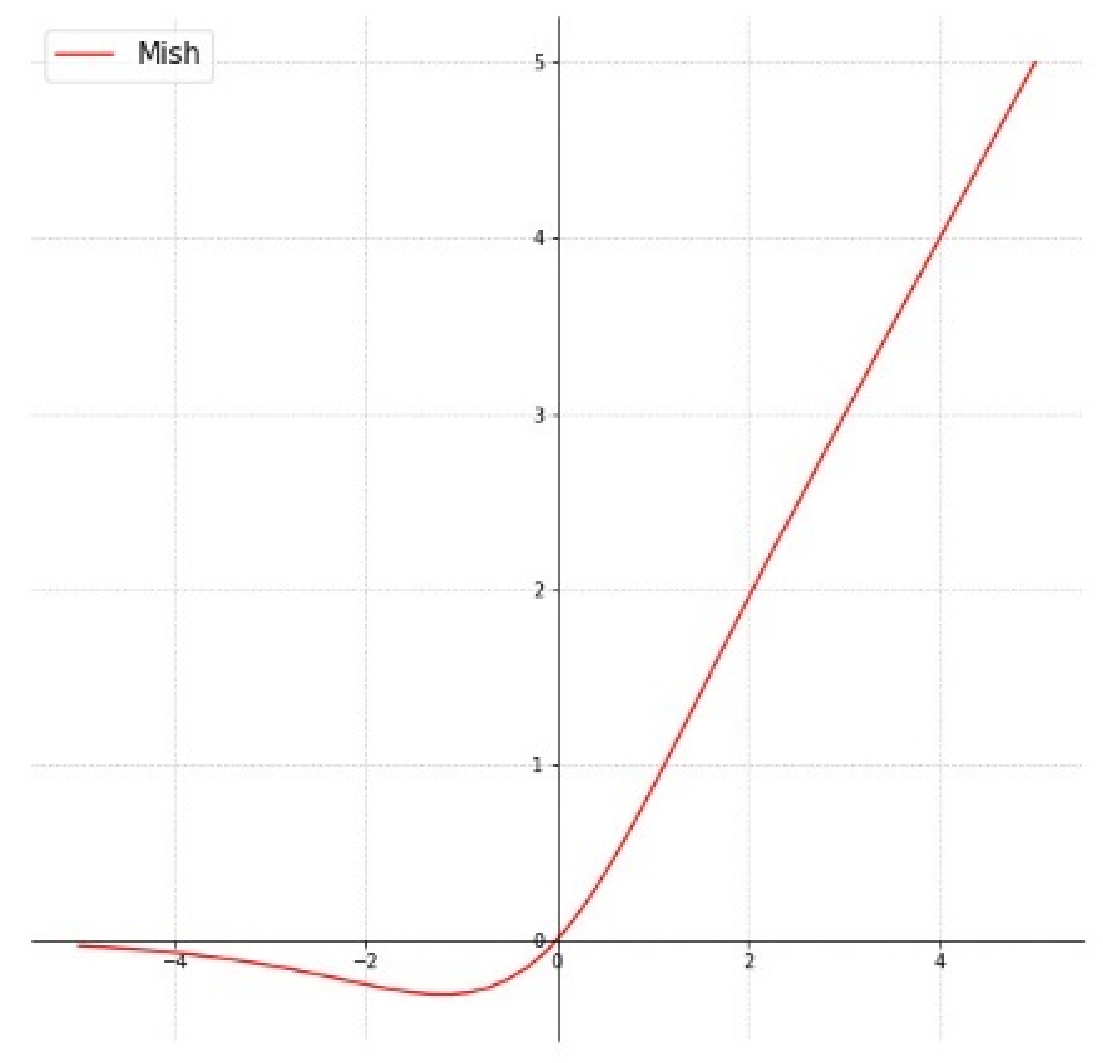
• The proposal of the MD-TinyYOLOv4 algorithm, which uses data augmentation, K-means++ clustering to optimize anchor box predictions, training with the Mish activation function instead of current functions such as ReLU or Leaky-ReLU and the addition of a dense SPP (Spatial Pyramid Pooling) network to accurately extract more features for the better detection of motorcycles near cars;
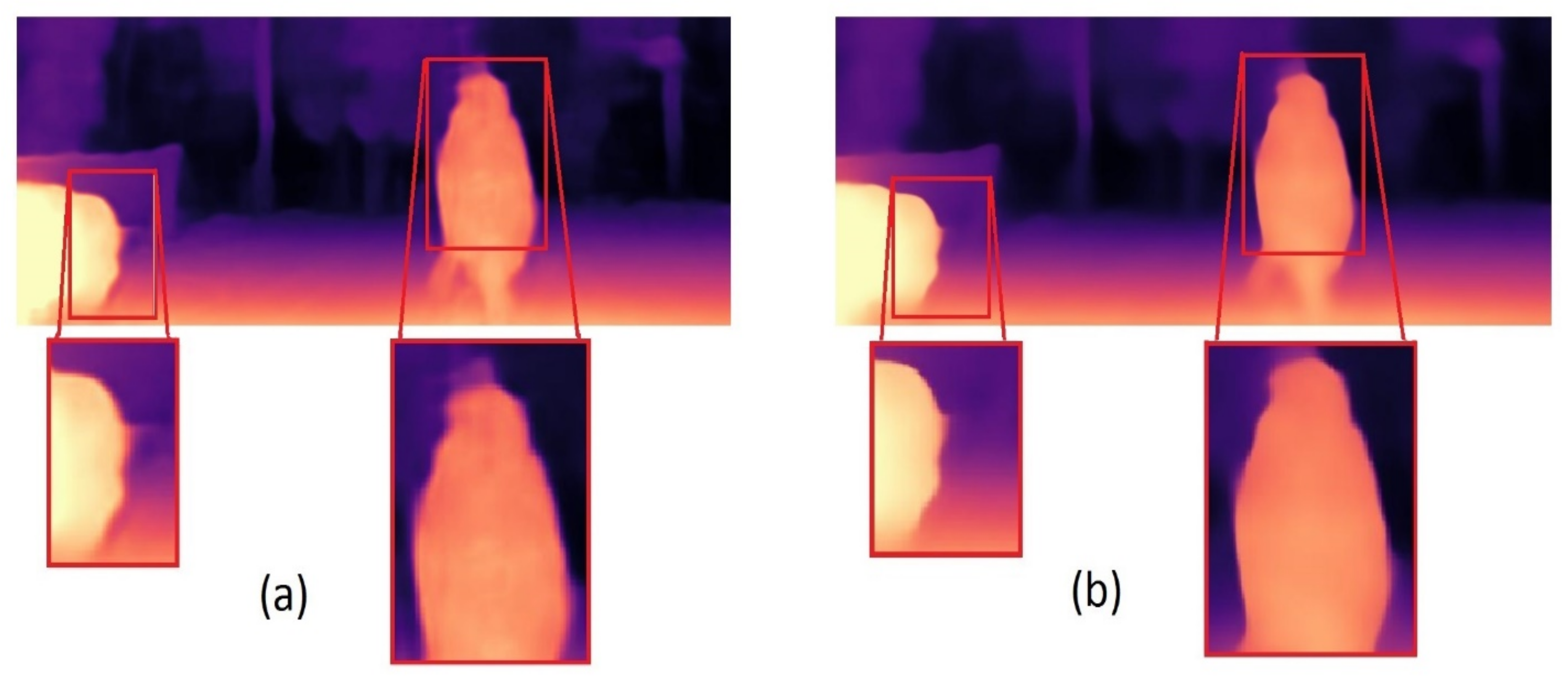
• The evaluation of the performances of Monodepth1 and Monodepth2 using our dataset and refinement using a joint bilateral filter to generate a disparity map with better visual quality and range value estimation;
• The provision of sufficient visualization results in classifying the condition of a motorcycle in the image as a dangerous or normal situation.

The following section (Section 2) presents the details of the proposed architecture, including the proposed MD-TinyYOLOv4 and Monodepth-based algorithms, as well as the captured remote sensing data for the methodology development and evaluation (Section 2.5). In Section 3, we provide a comprehensive description of the experimental results, with an analysis of the proposed motorcycle detection and range estimation models from monocular images. Finally, in the last section, the contributions and findings of this paper are summarized and some potential directions for future research are suggested.

2. Materials and Methods

The proposed methodology consisted of three main steps (Figure 2): (i) motorcycle detection, (ii) motorcycle depth estimation, and (iii) camera-to-motorcycle distance calculation. Finally, bounding boxes and computed distances were combined to provide (or not) an alert. The methodology was applied to images of both moving and stationary motorcycles acquired from a moving car.

For the motorcycle detection step (Section 2.1), several techniques were utilized to improve motorcycle detection, particularly for those with black windshields. These techniques include data augmentation, initial anchor box optimization, activation function modification, and backbone architecture improvement. In addition, refinement was applied to the disparity maps and the results were combined to estimate the range inside the motorcycle bounding box, which was then checked against a selected threshold.

For the motorcycle depth estimation step (Section 2.2), a state-of-the-art unsupervised monocular depth estimation model trained on a large-scale dataset was used to estimate the depth map of the detected motorcycle.

Finally, in the camera-to-motorcycle distance calculation step (Section 2.3), the distance between the camera and the motorcycle was calculated using the estimated depth map and the camera’s intrinsic and extrinsic parameters. This step enabled precise distance determination of the motorcycle from the camera in real-time.

The proposed methodology integrated object detection and depth estimation tasks to estimate the range of a motorcycle in real-time, even under challenging conditions. This approach addressed the limitations of previous studies and offered a promising solution for improving motorcycle safety in autonomous driving and smart navigation applications.

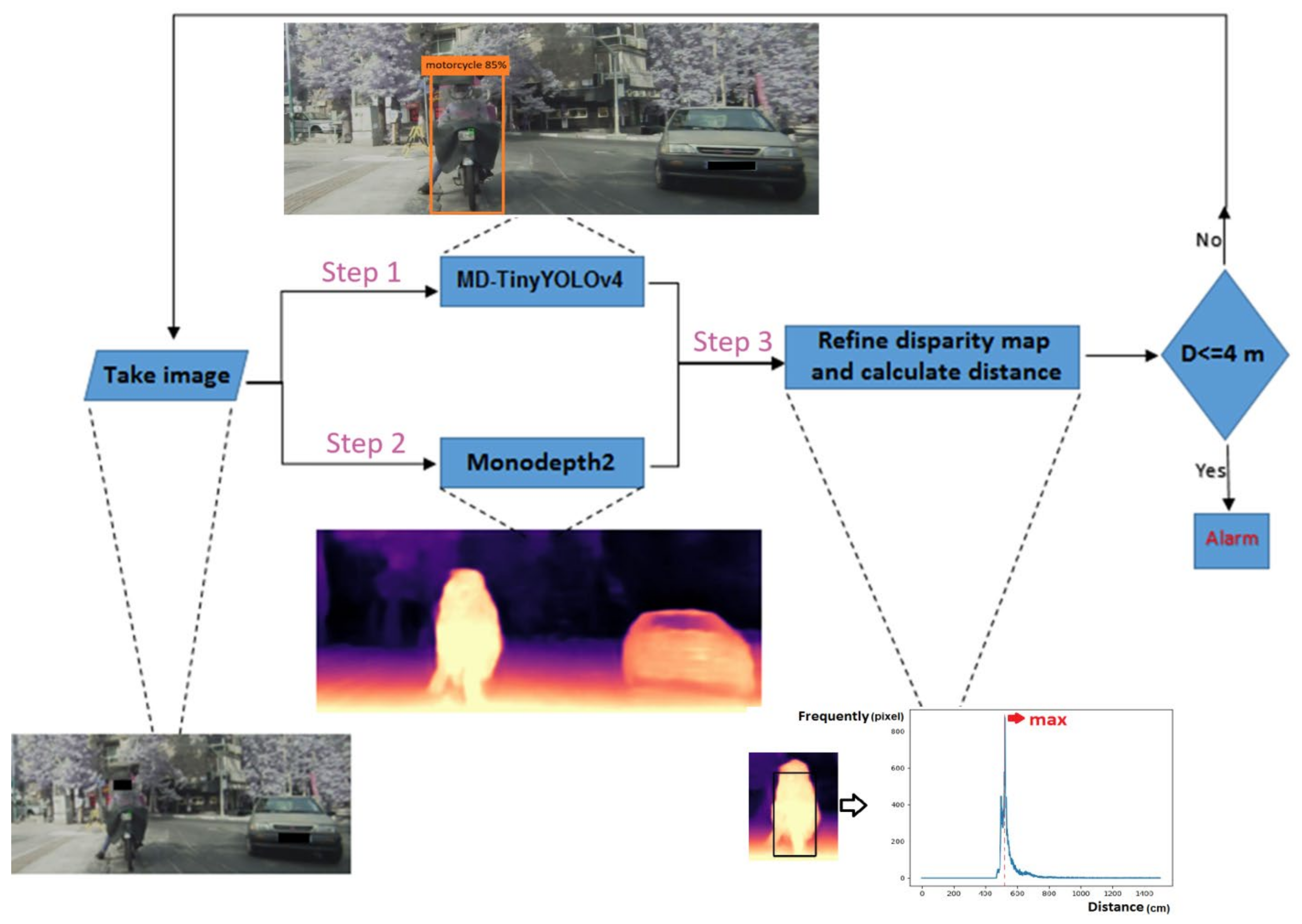
2.1. Motorcycle Detection with MD-TinyYOLOv4

YOLOv4 [28] is an improvement upon YOLOv3 and is composed of multiple convolutional layers, batch normalization, and activation functions. The tiny-YOLOv4 algorithm is a lightweight version of YOLOv4, one-tenth its size, that can detect a wide variety of objects in the MS-COCO dataset [62]. It includes twenty-two convolutional layers and three max-pooling layers. Unlike other YOLO types, tiny-YOLOv4 uses the CSPDarkNet-29 for feature extraction and C-IoU as a loss function during training. The Leaky-ReLU activation function is applied throughout the training of the algorithm. Compared to other tiny variants, such as tiny-YOLOv1, v2, and v3, tiny-YOLOv4 is the fastest algorithm that produces accurate detection results and is suitable for mobility services or embedded computing boards. However, the tiny-YOLOv4 algorithm struggles with detecting distinct tight bounding boxes and small objects. While some researchers have improved different types of YOLOv4 and tiny-YOLOv4 for vehicle detection [38] and bike recognition [63], regardless of their speed and accuracy, small and distant motorcycles with a black windshield are still challenging to detect. To address this challenge, we propose an MD-TinyYOLOv4 with a similar head and backbone to the tiny-YOLOv4 (Figure 3).

The initial dimensions of bounding boxes were calculated appropriately as part of our proposed detection model. Anchor boxes or prior boxes are a group of initial candidate boxes with a fixed value of width and height that directly affect the accuracy and processing time of the detection. The YOLOv3 and YOLOv4 models use YOLO detection layers that compute anchor box dimensions using K-means clustering [64]. However, inaccuracies in this clustering method can lead to wrong data points being grouped in a class, affecting the accuracy of the centroids chosen. To address this, we refined the clustering by using the K-means++ method [65], which independently initializes centroids and selects the optimum anchor box number to prevent network convergence during training. In K-means++, K random boxes are first chosen as cluster heads and in each repetition, anchor boxes are assigned around the nearest centroid. The next cluster center is then updated based on the highest anchor box probability [66]. The probabilities are computed based on Equation (1) [65]:

$$P=\frac{d{\left(x\right)}^2}{{{\displaystyle \sum }}_{i=1}^{n}d{\left(xi\right)}^2}$$

(1)

where d(x) is the direct distance obtained by evaluating the IOU (intersection over union) between each anchor box and the intended centroid. The procedure continues based on an IOU index as a threshold value until convergence. The full-scale YOLOv3 and YOLOv4 models use SPP [67] as an appropriate feature extraction network, which is not included in the CNN architecture of the tiny-YOLOv4. To improve distant motorcycle detection with more accurate bounding box estimation in our proposed MD-TinyYOLOv4, we added an SPP composed of 4 max-pooling layers with sizes of 3 × 3, 5 × 5, 7 × 7 and 9 × 9. After the 15th convolutional layer, the size of the produced feature map was converted from 13 × 13 × 512 to 13 × 13 × 2560 by the network.

The proposed detection model replaced the Leaky-ReLU activation function with the Mish function for better feature extraction in both the backbone and detection layers. Compared to other activation functions such as Sigmoid, ReLU, Leaky-ReLU, RReLU, ELU, GELU, SELU, SReLU, ISRU, and SoftPlus, the Mish function outperformed them with superior results [68]. The Leaky-ReLU has some limitations, such as continuity at zero, which can cause problems for gradient-based optimization [69]. Additionally, the low precision of the sigmoid during learning may lead to suboptimal performance and prevent the optimization from reaching local minimum values [70]. However, the Mish function was specifically designed to address these limitations by pushing signals to the left and right, making it easier to push feature creations toward their optimal point. Based on Equation (2), the Mish function has better expressivity and information flow due to its smooth and non-monotonic values.

$$f\left(x\right)=x.\tanh \left(\ln \left(1+e^x\right)\right)$$

(2)

As shown in Figure 4, the Mish function has unbounded above and bounded below properties that help to prevent saturation and result in strong regularization effects [28]. Furthermore, the infinite continuity of Mish is a significant advantage over ReLU and Leaky-ReLU, which have an order of continuity of 0 and can lead to undesired problems in gradient-based optimization. As reported in Section 3.2.1, the use of the Mish activation function in MD-TinyYOLOv4 resulted in a 5.4% and 4.8% accuracy increase compared to ReLU and Leaky-ReLU, respectively, in the detection of motorcycles.

Although YOLOv4 utilized various data augmentation techniques, none of them were used in the training of tiny-YOLOv4. Therefore, during the training process of MD-TinyYOLOv4, besides using some common augmentation methods, such as rotation, changing light, color space augmentation, and horizontal flip, the Mosaic and SAT data augmentation techniques were incorporated, enhancing the results. In this case, the combination of these techniques helps the model to become more robust to the surroundings of the objects and precisely detect the mentioned motorcycles.

Mosaic augmentation [28], illustrated in Figure 5, is a composite image technique that combines four images into one to improve training and identify objects at smaller scales. During the training, this method can help to avoid over-fitting and improve the optimal speed [71]. SAT is a technique that finds the part of the image on which the network relies most during training and is used to prevent overfitting in network training and increase model generalization. This technique involves changing the image by creating an oppositional attack on the current model, even if no objects are proposed in the image. Then, the model is trained with new images with their original bounding boxes and class labels. By incorporating these techniques, the MD-TinyYOLOv4 model is less likely to overfit and more likely to be applicable to a wider range of scenarios.

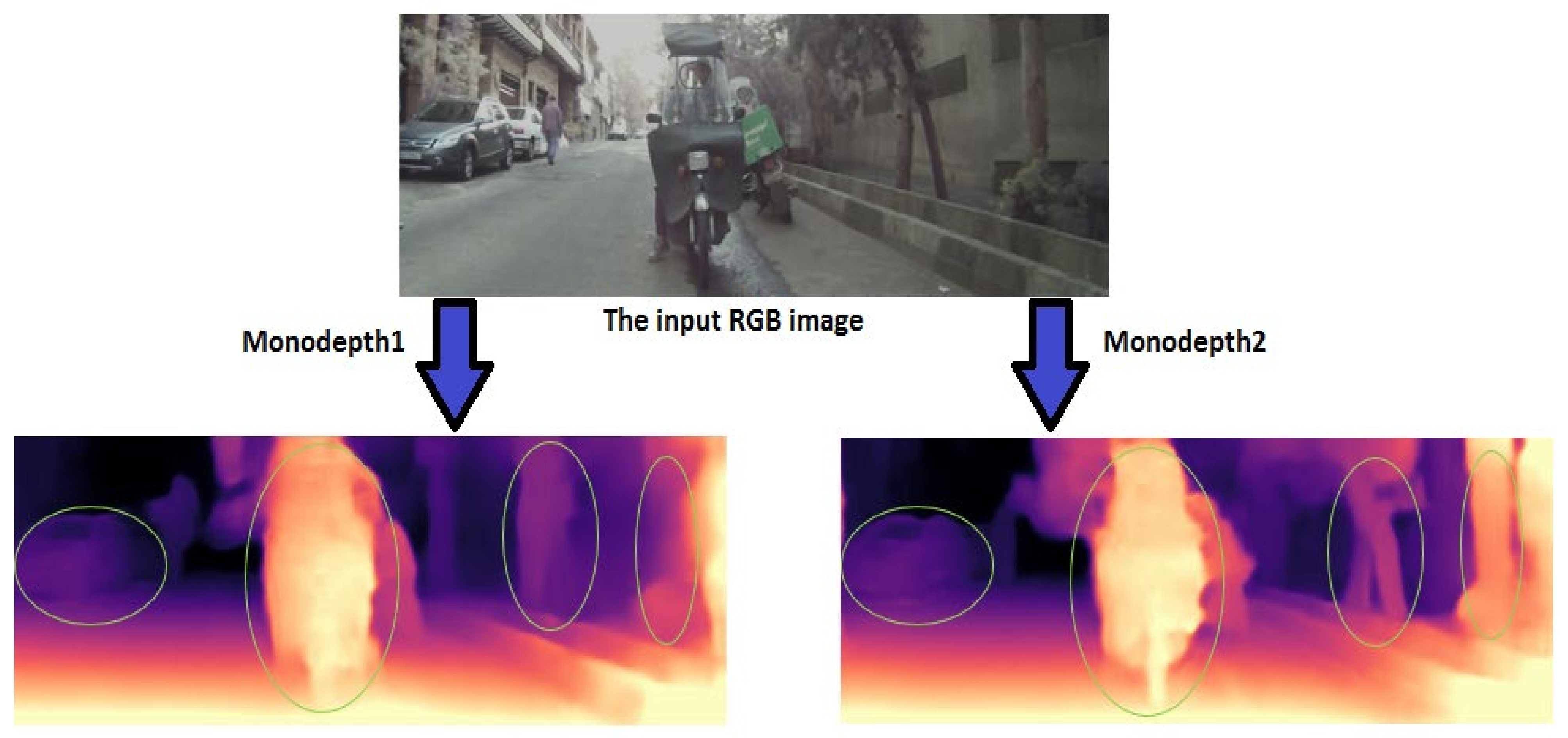
2.2. Monodepth for Depth Estimation

Range estimation should be performed at the same time as motorcycle detection in images from a monocular camera. Since collecting the ground truth depth data is a very big challenge in a wide range of environments, in 2017, a method called Monodepth was introduced [51]. In the Monodepth method, instead of using depth data or point cloud data as ground-truth data, the model uses RGB images as inputs for training both types of temporal images and the corresponding stereo pairs. For the purposes of training the mono frames, pose information and the depth networks are used alongside each other to learn the poses of the frames. However, this resulted in more errors compared to a stereo-pair known for reprojecting all frames from camera calibration. In this paper, two variants of the existing self-supervised approach, called Monodepth1 and Monodepth2 [51,60] were trained on a custom stereo-pair dataset of the Mynt-Eye camera. Based on their comparison, a relevant candidate for monocular depth prediction was chosen.

Monodepth1 is a 7-layer convolutional network for a single-image depth map estimation, regardless of scene geometry and the types of available features. For the purpose of predicting the depth, this network uses a multi-scale encoder–decoder through the different depth maps at each scale of the decoder being up-sampled to the reference input resolution [51]. The innovation of this method is in using the constraint related to the connection between the disparity maps made by the left and right images of the same scene. In the training phase, both the left image and the left disparity map are used for reconstructing the right image. Also, the left image can be reconstructed using the right image and its disparity map.

Monodepth2 [60] is an upgraded version of an unsupervised CNN-based approach that results in accurate depth estimation. Compared to the previous version, this model can better preserve the edges in the disparity map with a lower training time. This model has also described a depth prediction network and joint training loss for both detecting and looking at objects and predicting the final depth map from another viewpoint [60]. To predict a dense depth map (Dt) in this network, based on Equation (3), a combination of three main terms is used in the loss functions, namely the photometric reprojection error ($\underset{i}{\mathrm{L}}p$), the enforcement of disparity smoothness ($\underset{i}{\mathrm{L}}s$), and the consistency between the predicted left disparity map and right disparity map ($\underset{i}{\mathrm{L}}c$). As shown in Equation (4), the final loss function (L) is defined as the sum value of each ($\underset{i}{\mathrm{L}}$) in each of four different scales (I = 1, 2, 3, 4).

$$\underset{i}{\mathrm{Ls}}=\underset{i}{\mathrm{L}}p+\underset{i}{\mathrm{L}}s+\underset{i}{\mathrm{L}}c$$

(3)

$$L={{\displaystyle \sum }}_{i=1}^4\underset{i}{\mathrm{L}}s$$

(4)

Here, the photometric reprojection error (pre) causes the network to predict a dense depth map with a minimum of this error. Based on Equations (5) and (6) this loss function is combined with the least absolute deviations (L1) [72] and the structural similarity index (SSIM) [73] instead of a Gaussian function. Here, $I_{ij}$ is an input color image, ${\tilde{I}}_{\mathrm{ij}}$ is the reconstruction with respect to the target image $I_{ij}$, and N is the total number of all pixels in the image set to 0.85. Also, a significant improvement was applied to this reprojection error to increase the quality of the predicted depth. Therefore, based on Equation (7), the minimum photometric error among all images is used, which provides more accurate results by reducing the number of artifacts at image borders and more distinct sharp boundaries in occluded areas.

$$\mathrm{Lp} =\frac{1}{N}{\displaystyle \sum }_{ij}pre\left(I_{ij}, {\tilde{I}}_{\mathrm{ij}}\right)$$

(5)

$$pre\left(I_{ij}, {\tilde{I}}_{\mathrm{ij}}\right)=\frac{\mathsf{\alpha }}{2} \left(1-SSIM\left(I_{ij}, {\tilde{I}}_{\mathrm{ij}}\right)\right)+\left(1-\mathsf{\alpha }\right)\Vert I_{ij}-{\tilde{I}}_{\mathrm{ij}}\Vert$$

(6)

$$\mathrm{Lp} =\underset{t\prime }{\min }(pre\left(I_{ij}, {\tilde{I}}_{\mathrm{ij}}\right))$$

(7)

The disparity smoothness loss tries to locally smooth the discontinuities of the disparity map, which mostly occur at image gradients [74]. Therefore, $d^{*}$ is the predicted normalized disparity map, $I_{ij}$ is the input image, and ∂x and ∂y are, respectively, gradients of the input image in the x and y directions.

$$Ld=\frac{1}{N}{\displaystyle \sum }_{ij}\left|{\partial }_x{d}_{ij}^{*}\right| e^{-\Vert {\partial }_x{I}_{ij}\Vert }+\left|{\partial }_y{d}_{ij}^{*}\right| e^{-\Vert {\partial }_y{I}_{ij}\Vert }$$

(8)

$$d^{*}=\frac{d}{\overline{d}}$$

(9)

According to the consistency loss (L_C), the coherence between the two predicted disparity maps $d_{ij}^l$ and $d_{ij}^r$ is, respectively, calculated for the left and right images in order to better predict the disparity map.

$$Lc=\frac{1}{N}{{\displaystyle \sum }}_{ij}{\left|d\right.}_{ij}^l-\left.d_{ij}^r\right|$$

(10)

The source code of this model was written to train different free datasets such as Cityscape [75], ImageNet [76], and KITTI [77], which are accessible to all enthusiasts. The study of deep learning models has shown that if the model is trained by a compatible and rich database, an accurate depth map and relative distances of objects in the image will be achieved [78]. In these methods, instead of requiring an large dataset of images with known depth ground-truth data, a set of captured stereo images are used for the network fine-tuning with Mynt-Eye camera calibration parameters. These parameters are defined in Equation (11) within the K matrix as a camera intrinsic matrix in the training models. This matrix was normalized by the image size w × h. Here, fx and fy are the two elements of the focal length of the camera (in pixels) in the horizontal and vertical directions. u0 and v0 are the optical centers expressed in pixel coordinates.

$$K=\left[\begin{array}{cccc}fx/w& 0& u0/w& 0\\ 0& fy/h& v0/h& 0\\ 0& 0& 1& 0\\ 0& 0& 0& 1\end{array}\right]$$

(11)

2.3. Disparity Map Refinement

Errors and occlusion regions of the extracted disparity maps provided by Monodepth have a direct effect on the precision of the final result. Therefore, a joint bilateral filter was applied to rectify the error areas in the derived disparity map. This refinement technique tried to close holes in the disparity map, although it preserved the boundaries as the original image [79]. The equations of the joint bilateral filter are described in Equations (12) and (13) [80]:

$$D_p^{\prime }=\frac{1}{W_p} {\displaystyle \sum }_{q\in s}^n{G}_{{\sigma }_s}\left(\Vert p-q\Vert \right) G_{{\sigma }_r}\left(I_p-I_q\right)D_p$$

(12)

$$W_p=\frac{1}{W_p}{{\displaystyle \sum }}_{q\in s}^n{G}_{{\sigma }_s}\left(\Vert p-q\Vert \right) G_{{\sigma }_r}\left(I_p-I_q\right)$$

(13)

where D’_p is a generated pixel value when using a joint bilateral filter on the calculated depth map (D) and the intensity image (I). G_σs and G_σr are Gaussian functions with the mentioned parameters σs and σr, which define the size of the neighborhood. Also, s is a set of pixels that neighbor the p, and W_p is a constant for normalizing the equation.

In Monodepth, the weight parameters in the network are trained according to the camera calibration parameters [51]. Therefore, to achieve an accurate depth map on a single image, each image must be captured by a camera with intrinsic parameters similar to the camera parameters of the sensor used in the training dataset. To derive metric distances, Equation (14) is applied to convert the refined disparity map:

$$D=\frac{B\times f}{image\_size\times d}$$

(14)

where D is the followed distance, B is a baseline, and f is the focal length (in pixels) of the stereo images used for training. Also, in this model, the relative disparity output by the model must be scaled by the original image’s width.

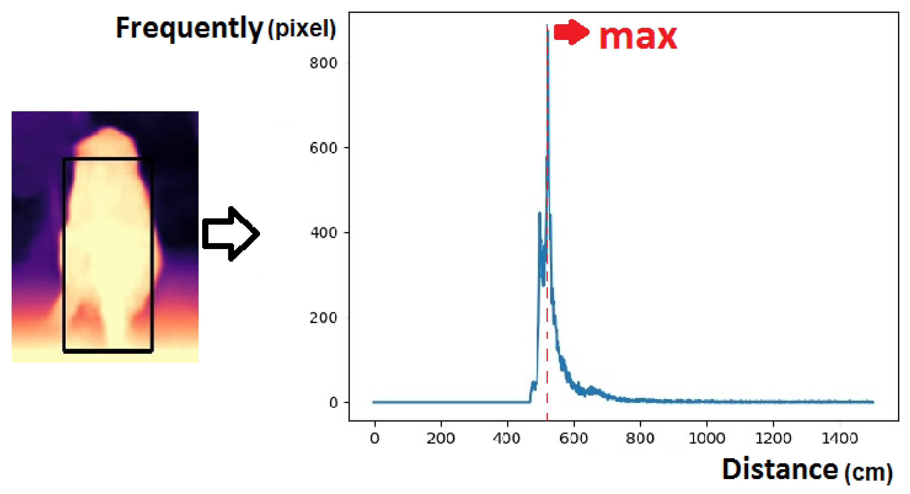
2.4. Combining Bounding Boxes and Disparity Maps

Finally, the refined disparity map is fused with the detected motorcycle boundary boxes to determine a single distance-to-camera value. Since the points captured from the front of the motorcycle are included as a set of points from the wheel to the upper windshield, it is not possible to simply define these recorded points on a single and flat surface. There are various models that can be used to select a single value as a candidate for all depth pixels of the detected bounding box. In this paper, as shown in Figure 6, a histogram of the pixel values is used to find the distance with the highest frequency and choose the most optimal depth value of pixels assigned to the motorcycle class in the image. If this distance value is lower than a chosen threshold, it will warn the driver about the presence of an approaching motorcycle. We experimentally chose 4 m as the minimum safe range threshold (Dt). If no danger is detected, the algorithm will jump to the next frame. This threshold can be changed according to the conditions and the type of vehicle.

2.5. Proposed Dataset

Detection and range estimation models used separate datasets during fine-tuning and training. Tehran (Iran) was chosen as the location for gathering images and collecting the datasets, as its roads have many motorcycles with black windshields. A generalization and extension of the datasets will be considered in the future.

2.5.1. Dataset for Motorcycle Detection

About 2000 images containing motorcycles with black windshields were captured as a training dataset. All these images were taken using an iPhone 8 camera from both moving and stationary motorcycles. This dataset was captured at different angles, distances, and scales during the day. All the images were resized to 416 × 416 px as the input size of the evaluation approach for the purposes of measuring the validity of the dataset. In the fine-tuning process, these images were randomly separated into 70% for the training, 10% for the validation, and 20% for testing. Flipping, rotating, mosaic, changing brightness, saturation, and contrast were some of the data augmentation techniques used. This helped object detectors to provide more features for better learning. Applying these techniques enhanced the size of our dataset by approximately 25%, which improved training and helped to avoid overfitting.

The LabelImg annotation tool [81] was used to annotate and extract distinct tight bounding boxes for each of the images. It was necessary to convert the XML data annotation files into VOC files first, which made a standardized image dataset for evaluating and comprising other methods. For each image, a text file with the same name was created. The class number, center coordinate of the bounding box (x and y), and image width and height were among the five parameters in each row of the text document.

2.5.2. Dataset for Motorcycle Range Estimation

The distance between the motorcycle and the front car was calculated using fine tuning and transfer learning from a Monodepth model. The images used in the training and testing phases were taken with the same camera and focal length [60]. The Monodepth model is trained using stereo images, while this model can ultimately estimate a disparity map from a single-color input image. Therefore, the training dataset was created using stereo images captured by the binocular Mynt-Eye camera (

Table 1. Mynt-Eye camera parameters [82].

Camera	Specifications	Parameters
Mynt-Eye D1000-IR-120/Color	Resolution	640 × 480 px
	Pixel size	3.75 µm
	Baseline	120 mm
	Focal Length	2.45 mm
	Visual Angle	D:121° H:105° V:58°
	Radial distortion parameters *	k1 = −0.3066, k2 = 0.00861
	Tangential distortion parameters *	p1 = −0.0003, p2 = 0.0015

The radial distortion parameters * and the tangential distortion parameters * came from the camera calibration process.

).

The dataset for depth estimation consisted of approximately 6000 pairs of rectified images of synchronized left and right frames. Images were captured from Tehran streets with varying traffic flows. Some preprocessing techniques, such as correcting radial and tangential distortion at the time of capture, were considered. Figure 7 shows an example of two pairs of these rectified images taken by the Mynt-Eye camera and used for network training. Images of different motorcycles with known distances between 0.3 and 7 m were taken with the Mynt-Eye camera with an accuracy of 0.02 m to evaluate the final alert results.

3. Results

The proposed MD-TinyYOLOv4 and the existing Monodepth models were trained and implemented using the Tensor Flow and PyTorch deep learning libraries. In the following subsection, we describe the evaluation parameters (Section 3.1) as well as the proposed model’s accuracy and prediction time (Section 3.2). All training and testing experiments were performed on an Ubuntu18.04 system with one GPU (GTX-1060, 16 GB RAM, and 6 GB VRAM).

As the most recent NVIDIA kits have a RAM of between 8 GB and 16 GB [83], in some existing autonomous vehicle applications, Jetson TX1 or Jetson Nano were used as accurate and fast devices for inferencing [84]. Therefore, based on the results and computational complexity of our model, the inference task can be run on these affordable devices instead of the super expensive and powerful systems used in some high-tech unmanned vehicles.

3.1. Evaluation Parameters

The results of the proposed algorithms are based on Equations (15)–(17), including Precision, Recall, and F1 score:

$$\mathrm{Precision}=\frac{\mathrm{TP}}{\mathrm{FP}+\mathrm{TP}}$$

(15)

$$\mathrm{Recall} =\frac{\mathrm{TP}}{\mathrm{FN}+\mathrm{TP}}$$

(16)

$$\mathrm{F}1 \mathrm{score} =2\times \frac{\mathrm{Recall}\times \mathrm{Precision}}{\mathrm{Recall}+\mathrm{Precision}}$$

(17)

$$\mathrm{RMSE}=\sqrt{\frac{1}{\mathrm{T}}{{\displaystyle \sum }}_{\mathrm{i}}^{\mathrm{T}}{\left({\mathrm{d}}_{\mathrm{i}}^{\mathrm{gt}}-{\mathrm{d}}_{\mathrm{i}}\right)}^2}$$

(18)

where TP indicates the true positive values, FP represents the false positive values and FN presents the false negative values. Also, for testing depth and distance results, as in Equation (18), the root means square error (RMSE) is obtained, which is almost a common indicator for evaluating range estimation methods. Here, d_i^gt is the real distance and d_i is the calculated distance of the motorcycle number i in the image.

3.2. Evaluation Results

According to the accuracies and speeds of different YOLO versions in detecting motorcycles, the proposed MD-TinyYOLOv4 model was optimized based on the original tiny-YOLOv4 model. Here, some of the key techniques were carefully hand-picked and verified, such as using anchor box optimization, adding an SPP layer in dense feature extraction, using data augmentation such as Mosaic and self-adversarial training (SAT), and using the Mish activation function. On the other hand, for depth estimation, the existing Monodepth models with a disparity map refinement were evaluated and compared based on the proposed dataset.

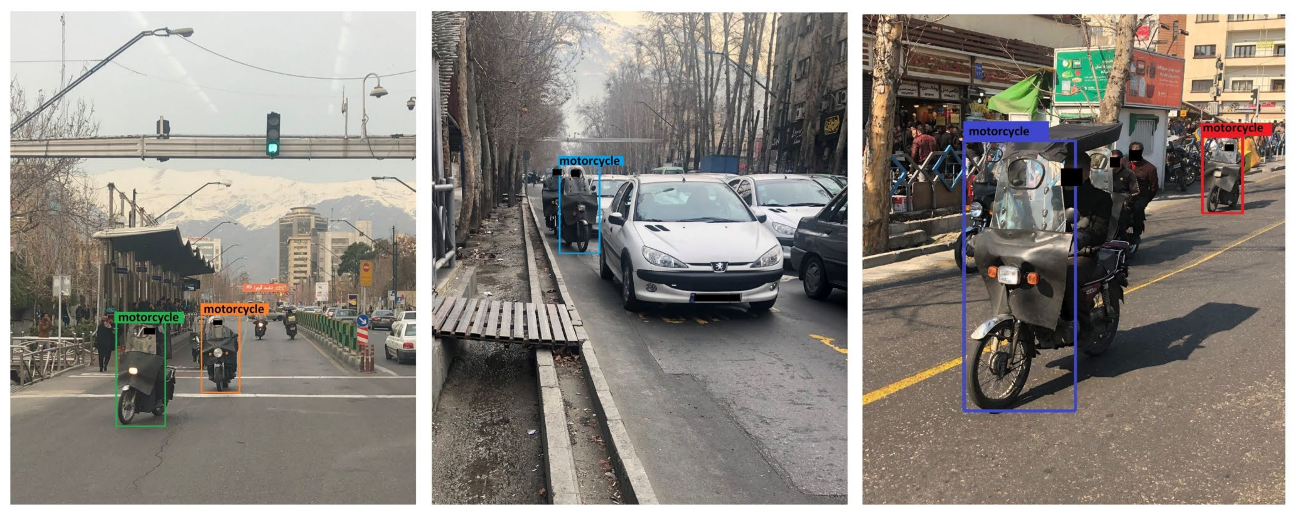
3.2.1. Proposed MD-TinyYOLOv4

The proposed MD-TinyYOLOv4 algorithm was compared with other existing original YOLO algorithms. For the purposes of testing the power and effectiveness of detecting motorcycles, the proposed method was trained on the captured dataset comprising images of motorcycles wearing black windshields on Tehran’s streets (Section 2.5.1). This training was conducted by defining the hyperparameters and initial variables as an input size of 416 × 416 px and a batch size value of 16. Also, the subdivision parameter and the momentum were, respectively, set to 8 and 0.9, with a learning rate of 0.015. These hyperparameters were handpicked, and we employed algorithms for training in 50 epochs until the confidence threshold met 0.25 with the IOU threshold reaching 50%. The timing procedure of this proposed model training took around 5 h for an appropriate 50 epochs. Before starting the training, anchor box optimization using K-means++ helps tune the object detector model to perform better detection of the small, large, and irregular objects in a dataset. This ascertains different numbers of centroids to find the ideal trade-off between the best IOU value and a sustainable training time. According to Figure 8, increasing the number of K directly affected the accuracy. Through experiments, K = 10 achieved the most optimal average IOU = 87.2%, considering a fine balance between model complication and its performance. In Figure 9, the forms and dimensions of 10 predicted anchor boxes based on the proposed dataset are shown. The values of these anchor boxes calculated via K-means++ clustering are as follows: (12, 21), (15, 34), (20, 49), (30, 60), (35, 77), (40, 95), (52, 117), (70, 155), (115, 250), (155, 352).

The evaluation of the proposed MD-TinyYOLOv4 model and the comparison results with the existing YOLO variants and SSD (Single Shot Detector) models are shown in

Table 2. Inference evaluation of different YOLO versions and SSD architectures based on our dataset.

Version	Precision	Recall	F1 Score	Motorcycle Position		Time Forecast
				Close	Far
YOLOv1	0.64	0.53	0.579	✓	×	40 FPS
YOLOv2	0.67	0.61	0.63	✓	×	40 FPS
SSD512	0.68	0.66	0.60	✓	×	28
SSD300	0.71	0.78	0.77	✓	×	25
YOLOv3	0.69	0.75	0.77	✓	×	30 FPS
YOLOv4	0.75	0.79	0.79	✓	✓	35 FPS
Tiny-YOLOv1	0.3	0.43	0.35	✓	×	120 FPS
Tiny-YOLOv2	0.45	0.48	0.46	✓	×	200 FPS
Tiny-YOLOv3	0.60	0.59	0.63	✓	×	220 FPS
Tiny-YOLOv4	0.7	0.6	0.64	✓	✓	240 FPS
MD-TinyYOLOv4	0.81	0.79	0.79	✓	✓	240 FPS

. Different SSD architectures may have varying levels of accuracy and speed [25]. There are several versions of SSD models, such as SSD300 and SSD512, each with various compromises between speed and precision. The low-resolution SSD300 model was about 3% more accurate than SSD512. According to the proposed dataset and results obtained via comparison with the YOLO variants, the SSD300 performed very similarly to YOLOv3 in this case. On the other hand, in cases of hardware limitations, SSD300 could be a suitable option, with a balance between speed and accuracy.

However, the YOLOv4 model outperformed these results by achieving a precision of 75%, the highest precision among other original variants in detecting motorcycles with a black windshield. This means that the prepared dataset is appropriate for the detection of motorcycles with different appearances, as they have a variety of sizes based on their location in the street. On the other hand, different variants of the tiny-YOLO algorithms have lower computation resource requirements and a higher speed in object detection because of having a smaller feature extraction network. However, when comparing original tiny variants based on the proposed dataset, the original tiny-YOLOv4 also performed with better accuracy, with the highest precision of 70%. Based on the importance of computation resource limitations in ADAS applications and achieving better performance in using existing tiny variants based on the proposed dataset, a refinement of tiny-YOLOv4 with the name of MD-TinyYOLOv4 achieved accuracy values 11% higher than the accuracy of the original tiny-YOLOv4 model. Although the proposed MD-TinyYOLOv4 model seems to have similar results to YOLOv4, the prediction speed is approximately seven times that of YOLOv4 when tested on the custom dataset. These improvements mean that the proposed MD-TinyYOLOv4 is more capable of detecting distant and smaller motorcycles with higher precision and sufficient processing speed, as in Figure 10, results of detecting motorcycles in different distances and street congestion can be seen. Additionally, the MD-TinyYOLOv4 model can better detect distant or small motorcycles appearing in different road conditions.

3.2.2. Disparity and Depth Map Extracting

Monodepth1 and Monodepth2 had already been trained based on the ImageNet and KITTI datasets. In our work, these existing pretrained weights were used as the initial parameters for fine-tuning models in 100 epochs based on the proposed datasets. In Figure 11, three samples from Image-net, KITTI, and the proposed datasets are shown. Based on this comparison, KITII is more similar to the database prepared in this paper. The results also proved that by fine-tuning the network with pretrained weights from the KITTI dataset, the network performances increased by 43% in terms of accuracy compared with fine-tuning with the existing pretrained weights of the ImageNet dataset.

As shown in Figure 12, the disparity map produced by Monodepth2 has better and sharper results in displaying motorcycle edges and narrower features in comparison with Monodepth1. The improved results are due to the cost functions used in the training model and also in upsampling the resolution of the disparity map, which was changed according to the resolution of the original input image.

After the disparity map is obtained using the fine-tuned Monodepth model, the joint bilateral filter is applied to obtain better disparity values. According to the results reported in

Table 3. The evaluation of different fine-tuned Monodepth2 models.

Disparity Map Model	Disparity Filter	Pretrained Weight	Distance RMSE (m)	Runtime
Monodepth1	None	ImageNet	0.8346	35 fps or 0.028 s
	Joint bilateral filter		0.7739
Monodepth1	None	KITTI	0.4756	35 fps or 0.028 s
	Joint bilateral filter		0.416
Monodepth2	None	ImageNet	0.6868	45 fps or 0.022 s
	Joint bilateral filter		0.6061
Monodepth2	None	KITTI	0.3620	45 fps or 0.022 s
	Joint bilateral filter		0.323

, the refined disparity map derived with the Monodepth2 model on the proposed dataset achieved almost 20% less RMSE than the previous Monodepth1, which means that the estimated distances were close to the actual values. Also, the time prediction of the disparity map by Monodepth2 was almost 1.28 times faster than the previous Monodepth1 version. The mentioned refinement helps to rectify errors and the noise region around the object boundaries. This filter achieves an RMSE of 0.323 m in the distances calculated from a refined disparity map of Monodepth2, which used pre-trained weights of the KITTI dataset in the training process.

Figure 13 shows a sample of the proposed dataset with the improvements to the proposed disparity map refinement. Because of some errors in disparity values, the occlusion area and the boundary region of objects have problems with blurring and unclear shapes.

3.2.3. Evaluating the Proposed Algorithm at Different Distances and Conditions

The main aim of this work is to deliver a methodology for monitoring and alarming drivers before reaching a dangerous distance from a motorcycle. The methodology was tested and performed in different road conditions with different traffic flows. Different images in different conditions, such as sunny, cloudy, and rainy weather, were also checked. However, the weather directly affects the performance of both algorithms: the most accurate results were achieved in a convenient lighting scene without too many shadows and reflectance phenomena in the image. Also, the evaluation and the final results were based on applying the algorithm to all scenarios where the motorcycle is fully seen in the image. This algorithm specifically worked on a special set of images of motorcycles with black windshields, and therefore in the case of partially covered motorcycles behind other vehicles, the anchor box detection and the range estimation algorithms faced many more problems and produced false results. This may need some extra inclusive data or human input. However, YOLOv4 performed 12% better in detecting enclosed and partially seen motorcycles compared to MD-TinyYOLOv4. To examine the proposed algorithm at different distances and conditions, the ground-truth distance was collected and measured in ranges between 0.3 m and 7 m, as shown in Figure 14.

According to the achieved results, in the range under 4 m, a greater RMSE can be seen in comparison to the range between 4 and 7 m. This happens because, at ranges smaller than 4 m, the motorcycle is too close to the camera, and so a large part of the image includes the motorcycle shape with an insufficient view of the background. In this situation, the algorithm will not be able to properly estimate the depth. In addition, the shorter distance of the motorcycle to the camera causes an increase in the parallax of the motorcycle, which will increase the algorithm error. The average relative errors in calculating distances below 4 m were estimated as being up to 0.36 m. However, in the range of 4–7 m, the algorithm estimates the position and distance of the motorcycle with an average RMSE of approximately 0.28 m at 46 fps for every single image, which is equal to the processing time of some intelligent systems of traffic enforcement cameras. The average time taken to process each region of interest was 71 ms for Siebert [11], 50 ms for Deigmoeller et al. [85], 37 ms for Shine [86], and 22 ms for our method.

The contributions of the MD-TinyYOLOv4 model and Monodepth2 were examined under normal conditions. Half of all these images captured motorcycles that were in the dangerous ranges (distances below 4 m), and the other half captured motorcycles further than 4 m from the camera. According to the results, the proposed tested model correctly detected 86% of simulated alarm cases and recognized 92% of cases as true normal situations. This proposed alarm algorithm can be performed in real time with an average speed of 40 fps on a custom dataset, promising to be suitable as a real-time method.

Figure 15 shows the detection results for motorcycles that are estimated as being too close with respect to warning conditions. In these warning cases, the motorcycle bounding box color changes to red to attract more attention. Contrarily, results for normal situations are shown with green bounding boxes, i.e., the detected motorcycles are at a safe distance from the camera.

4. Discussion

The study of existing visual ADAS models indicates that using single models for both detection and range estimation is not effective in estimating distances due to the supervised learning methods and the difficulties in recording training data with different devices such as RTK-GNSS, LIDAR, etc. On the other hand, based on their published results, they were unable to achieve the level of precision and speed required in this article. Therefore, the best way to solve this problem was to investigate and refine the detection and distance estimation as two consecutive separate methods. In this case, prior to estimating distances, it is essential to establish accurate knowledge of the location and bounding box of the motorcycle. As we only wanted to detect one class (as a motorcycle with a black windshield) and then perform subsequent distance estimation, a refined model, MD-TinyYOLOv, was the best choice among SSD and all other YOLO versions. The proposed model improved the detection accuracy while maintaining the appropriate time taken and accurate detection input for the rest of the distance estimation model. Among other famous distance estimation methods using single images, such as linear regression, pinhole, and deep learning models, the refined Monodepth2 model was used as the best algorithm in this application due to its consistency in prediction and its independence from changes in camera calibration parameters and road conditions. This model identifies all non-linear relations between the input image and the estimated depth map with a reasonable standard deviation, which is impossible to achieve in other linear regression or pinhole methods. The assessment of the detection output revealed that on occasion, either the entire or a portion of the estimated depth map was unreliable and false, which might be related to motorcycle occlusion or adverse weather conditions and ambient lighting.

5. Conclusions

This joined remote sensing and AI-based study proposed an integrated methodology for motorcycle detection and range estimation using a single camera installed on the back of a vehicle. Since motorcycles are small objects in these images relative to other road objects like vehicles or buses, the YOLO object detectors were considered a priority. This study provides a dataset of motorcycles in different scenarios and conditions and presents the MD-TinyYOLOv4 model for motorcycle detection. The proposed method outperforms the original tiny-YOLOv4 by 10.8%. The work also refines the architecture of the tiny-YOLOv4 model with different modifications for distant and small motorcycles. For range estimation, a comparative study is carried out between two state-of-the-art models, Monodepth1 and Monodepth2, using a stereo dataset captured using a Mynt-Eye camera. The proposed integrated methodology has great implications for motorcycle safety, as experiments showed that 86% of simulated situations where motorcycles were closer than 4 m were correctly recognized as alarm situations. The methodology’s code and datasets will be shared with the community upon the acceptance of this paper.

Future studies will improve the proposed method by applying object detection and depth estimation models to other road users, with other windshields, and with vehicle behavior prediction and movement. Further investigation should generalize the methodology based on images from different types of camera parameters as, so far, the methodology derives metric distances only from calibrated cameras. Finally, since our approach is not capable of handling nighttime scenes, detection and distance estimation in (partly) nighttime scenarios should be considered.

References

1. Markiewicz, P.; Długosz, M.; Skruch, P. Review of tracking and object detection systems for advanced driver assistance and autonomous driving applications with focus on vulnerable road users sensing. In Proceedings of the Polish Control Conference, Kraków, Poland, 18–21 June 2017; Springer: Cham, Switzerland, 2017; pp. 224–237. [Google Scholar]
2. Pineda-Deom, D. Motorcycle Blind Spot Detection System and Rear Collision Alert Using Mechanically Aligned Radar. U.S. Patent 10,429,501, 1 October 2019. [Google Scholar]
3. Anaya, J.J.; Ponz, A.; García, F.; Talavera, E. Motorcycle detection for ADAS through camera and V2V Communication, a comparative analysis of two modern technologies. Expert Syst. Appl. 2017, 77, 148–159. [Google Scholar] [CrossRef]
4. De Raeve, N.; De Schepper, M.; Verhaevert, J.; Van Torre, P.; Rogier, H. A bluetooth-low-energy-based detection and warning system for vulnerable road users in the blind spot of vehicles. Sensors 2020, 20, 2727. [Google Scholar] [CrossRef] [PubMed]
5. Gruyer, D.; Rahal, M.-C. Multi-Layer Laser Scanner Strategy for Obstacle Detection and Tracking. In Proceedings of the 2019 IEEE/ACS 16th International Conference on Computer Systems and Applications (AICCSA), Abu Dhabi, United Arab Emirates, 3–7 November 2019; IEEE: Piscataway, NJ, USA; pp. 1–8. [Google Scholar]
6. Gong, D.-W.; Dai, X.; Chen, Y.; Wang, S.-F. Single-layer Laser Scanner-based Approach for a Transportation Participants Recognition Task. Lasers Eng. 2019, 43, 10–12. [Google Scholar]
7. Kim, J.B. Efficient vehicle detection and distance estimation based on aggregated channel features and inverse perspective mapping from a single camera. Symmetry 2019, 11, 1205. [Google Scholar] [CrossRef]
8. Haseeb, M.A.; Guan, J.; Ristic-Durrant, D.; Gräser, A. Disnet: A novel method for distance estimation from monocular camera. In Proceedings of the 10th Planning, Perception and Navigation for Intelligent Vehicles (PPNIV18), Madrid, Spain, 1 October 2018. [Google Scholar]
9. Vajgl, M.; Hurtik, P.; Nejezchleba, T. Dist-YOLO: Fast Object Detection with Distance Estimation. Appl. Sci. 2022, 12, 1354. [Google Scholar] [CrossRef]
10. Vishnu, C.; Singh, D.; Mohan, C.K.; Babu, S. Detection of motorcyclists without helmet in videos using convolutional neural network. In Proceedings of the 2017 International Joint Conference on Neural Networks (IJCNN), Anchorage, AK, USA, 14–19 May 2017; IEEE: Piscataway, NJ, USA; pp. 3036–3041. [Google Scholar]
11. Siebert, F.W.; Lin, H. Detecting motorcycle helmet use with deep learning. Accid. Anal. Prev. 2020, 134, 105319. [Google Scholar] [CrossRef]
12. Sanchana, M.A.; Eliyas, S. Automated Motorcycle Helmet Detection Using The Combination of YOLO AND CNN. In Proceedings of the 2023 3rd International Conference on Advance Computing and Innovative Technologies in Engineering (ICACITE), Greater Noida, India, 12–13 May 2023; IEEE: Piscataway, NJ, USA; pp. 75–77. [Google Scholar]
13. Sridhar, P.; Jagadeeswari, M.; Sri, S.H.; Akshaya, N.; Haritha, J. Helmet violation detection using YOLO v2 deep learning framework. In Proceedings of the 2022 6th International Conference on Trends in Electronics and Informatics (ICOEI), Tirunelveli, India, 28–30 April 2022; IEEE: Piscataway, NJ, USA; pp. 1207–1212. [Google Scholar]
14. Mistry, J.; Misraa, A.K.; Agarwal, M.; Vyas, A.; Chudasama, V.M.; Upla, K.P. An automatic detection of helmeted and non-helmeted motorcyclist with license plate extraction using convolutional neural network. In Proceedings of the 2017 Seventh International Conference on Image Processing Theory, Tools and Applications (IPTA), Montreal, QC, Canada, 28 November–1 December 2017; IEEE: Piscataway, NJ, USA; pp. 1–6. [Google Scholar]
15. Laroca, R.; Severo, E.; Zanlorensi, L.A.; Oliveira, L.S.; Gonçalves, G.R.; Schwartz, W.R.; Menotti, D. A robust real-time automatic license plate recognition based on the YOLO detector. In Proceedings of the 2018 International Joint Conference on Neural Networks (IJCNN), Rio de Janeiro, Brazil, 8–13 July 2018; IEEE: Piscataway, NJ, USA; pp. 1–10. [Google Scholar]
16. Rao, Y.A.; Kumar, S.; Amaresh, H.; Chirag, H. Real-time speed estimation of vehicles from uncalibrated view-independent traffic cameras. In Proceedings of the TENCON 2015—2015 IEEE Region 10 Conference, Macao, China, 1–4 November 2015; IEEE: Piscataway, NJ, USA; pp. 1–6. [Google Scholar]
17. Luvizon, D.C.; Nassu, B.T.; Minetto, R. A video-based system for vehicle speed measurement in urban roadways. IEEE Trans. Intell. Transp. Syst. 2016, 18, 1393–1404. [Google Scholar] [CrossRef]
18. Chang, I.-C.; Yen, C.-E.; Song, Y.-J.; Chen, W.-R.; Kuo, X.-M.; Liao, P.-H.; Kuo, C.; Huang, Y.-F. An Effective YOLO-Based Proactive Blind Spot Warning System for Motorcycles. Electronics 2023, 12, 3310. [Google Scholar] [CrossRef]
19. Strbac, B.; Gostovic, M.; Lukac, Z.; Samardzija, D. YOLO multi-camera object detection and distance estimation. In Proceedings of the 2020 Zooming Innovation in Consumer Technologies Conference (ZINC), Novi Sad, Serbia, 26–27 May 2020; IEEE: Piscataway, NJ, USA; pp. 26–30. [Google Scholar]
20. Espinosa, J.E.; Velastin, S.A.; Branch, J.W. Motorcycle detection and classification in urban Scenarios using a model based on Faster R-CNN. arXiv 2018, arXiv:1808.02299. [Google Scholar]
21. Girshick, R.; Donahue, J.; Darrell, T.; Malik, J. Rich feature hierarchies for accurate object detection and semantic segmentation. In Proceedings of the 2014 Computer Vision and Pattern Recognition (CVPR), Columbus, OH, USA, 23–28 June 2014; IEEE: Piscataway, NJ, USA; pp. 580–587. [Google Scholar]
22. Girshick, R. Fast R-CNN. In Proceedings of the 2015 International Conference on Computer Vision (ICCV), Santiago, Chile, 7–13 December 2015; pp. 1440–1448. [Google Scholar]
23. Ren, S.; He, K.; Girshick, R.; Sun, J. Faster r-cnn: Towards real-time object detection with region proposal networks. In Proceedings of the Advances in Neural Information Processing Systems, Montreal, QC, Canada, 7–12 December 2015; pp. 91–99. [Google Scholar]
24. Chen, Z.; Khemmar, R.; Decoux, B.; Atahouet, A.; Ertaud, J.-Y. Real Time Object Detection, Tracking, and Distance and Motion Estimation based on Deep Learning: Application to Smart Mobility. In Proceedings of the 2019 Eighth International Conference on Emerging Security Technologies (EST), Colchester, UK, 22–24 July 2019; IEEE: Piscataway, NJ, USA; pp. 1–6. [Google Scholar]
25. Liu, W.; Anguelov, D.; Erhan, D.; Szegedy, C.; Reed, S.; Fu, C.-Y.; Berg, A.C. Ssd: Single shot multibox detector. In Proceedings of the 14th European Conference on Computer Vision, Amsterdam, The Netherlands, 11–14 October 2016; pp. 21–37. [Google Scholar]
26. Redmon, J.; Farhadi, A. YOLO9000: Better, faster, stronger. In Proceedings of the IEEE Conference on Computer Vision and Pattern Recognition, Honolulu, HI, USA, 21–26 July 2017; pp. 7263–7271. [Google Scholar]
27. Redmon, J.; Farhadi, A. Yolov3: An incremental improvement. arXiv 2018, arXiv:1804.02767. [Google Scholar]
28. Bochkovskiy, A.; Wang, C.-Y.; Liao, H.-Y.M. YOLOv4: Optimal Speed and Accuracy of Object Detection. arXiv 2020, arXiv:2004.10934. [Google Scholar]
29. Redmon, J.; Divvala, S.; Girshick, R.; Farhadi, A. You only look once: Unified, real-time object detection. In Proceedings of the IEEE Computer Society Conference on Computer Vision and Pattern Recognition, Las Vegas, NV, USA, 27–30 June 2016; IEEE: Piscataway, NJ, USA; pp. 779–788. [Google Scholar]
30. Jamtsho, Y.; Riyamongkol, P.; Waranusast, R. Real-time license plate detection for non-helmeted motorcyclist using YOLO. ICT Express 2021, 7, 104–109. [Google Scholar] [CrossRef]
31. Kumar, A.; Kalia, A.; Verma, K.; Sharma, A.; Kaushal, M. Scaling up face masks detection with YOLO on a novel dataset. Optik 2021, 239, 166744. [Google Scholar] [CrossRef]
32. Kumar, A.; Kalia, A.; Kalia, A. ETL-YOLO v4: A face mask detection algorithm in era of COVID-19 pandemic. Optik 2022, 259, 169051. [Google Scholar] [CrossRef] [PubMed]
33. Chen, R.-C. Automatic License Plate Recognition via sliding-window darknet-YOLO deep learning. Image Vis. Comput. 2019, 87, 47–56. [Google Scholar]
34. Rani, E. LittleYOLO-SPP: A delicate real-time vehicle detection algorithm. Optik 2021, 225, 165818. [Google Scholar]
35. Yi, Z.; Yongliang, S.; Jun, Z. An improved tiny-yolov3 pedestrian detection algorithm. Optik 2019, 183, 17–23. [Google Scholar] [CrossRef]
36. Everingham, M.; Van Gool, L.; Williams, C.K.; Winn, J.; Zisserman, A. The pascal visual object classes (voc) challenge. Int. J. Comput. Vis. 2010, 88, 303–338. [Google Scholar] [CrossRef]
37. Bhujbal, A.; Mane, D. Vehicle Type Classification Using Deep Learning. In Proceedings of the International Conference on Soft Computing and Signal Processing, Hyderabad, India, 21–22 June 2019; pp. 279–290. [Google Scholar]
38. Mahto, P.; Garg, P.; Seth, P.; Panda, J. Refining Yolov4 for Vehicle Detection. Int. J. Adv. Res. Eng. Technol. 2020, 11, 409–419. [Google Scholar]
39. Thuan, D. Evolution of yolo Algorithm and yolov5: The State-of-the-Art Object Detection Algorithm. Bachelor’s Thesis, Oulu University, Oulu, Finland, 2021. [Google Scholar]
40. Huang, Y.; Zhang, H. A Safety Vehicle Detection Mechanism Based on YOLOv5. In Proceedings of the 2021 IEEE 6th International Conference on Smart Cloud (SmartCloud), Newark, NJ, USA, 6–8 November 2021; IEEE: Piscataway, NJ, USA; pp. 1–6. [Google Scholar]
41. Jiang, P.; Ergu, D.; Liu, F.; Cai, Y.; Ma, B. A Review of Yolo Algorithm Developments. Procedia Comput. Sci. 2022, 199, 1066–1073. [Google Scholar] [CrossRef]
42. Fanthony, I.V.; Husin, Z.; Hikmarika, H.; Dwijayanti, S.; Suprapto, B.Y. YOLO Algorithm-Based Surrounding Object Identification on Autonomous Electric Vehicle. In Proceedings of the 2021 8th International Conference on Electrical Engineering, Computer Science and Informatics (EECSI), Semarang, Indonesia, 20–21 October 2021; IEEE: Piscataway, NJ, USA; pp. 151–156. [Google Scholar]
43. Chen, Y.-C.; Su, T.-F.; Lai, S.-H. Integrated vehicle and lane detection with distance estimation. In Proceedings of the Computer Vision ACCV 2014 Workshops, Singapore, 1–2 November 2014; pp. 473–485. [Google Scholar]
44. Xing, Y.; Lv, C.; Chen, L.; Wang, H.; Wang, H.; Cao, D.; Velenis, E.; Wang, F.-Y. Advances in vision-based lane detection: Algorithms, integration, assessment, and perspectives on ACP-based parallel vision. IEEE/CAA J. Autom. Sin. 2018, 5, 645–661. [Google Scholar] [CrossRef]
45. Kang, C.; Heo, S.W. Intelligent safety information gathering system using a smart blackbox. In Proceedings of the 2017 IEEE International Conference on Consumer Electronics (ICCE), Las Vegas, NV, USA, 8–10 January 2017; IEEE: Piscataway, NJ, USA; pp. 229–230. [Google Scholar]
46. Mahmoud, N.; Cirauqui, I.; Hostettler, A.; Doignon, C.; Soler, L.; Marescaux, J.; Montiel, J.M.M. ORBSLAM-based endoscope tracking and 3D reconstruction. In Proceedings of the International Workshop on Computer-Assisted and Robotic Endoscopy, Athens, Greece, 17 October 2017; pp. 72–83. [Google Scholar]
47. Schonberger, J.L.; Frahm, J.-M. Structure-from-motion revisited. In Proceedings of the 2016 IEEE Conference on Computer Vision and Pattern Recognition, Las Vegas, NV, USA, 27–30 June 2016; pp. 4104–4113. [Google Scholar]
48. Smith, M.W.; Carrivick, J.L.; Quincey, D.J. Structure from motion photogrammetry in physical geography. Prog. Phys. Geogr. 2016, 40, 247–275. [Google Scholar] [CrossRef]
49. Chwa, D.; Dani, A.P.; Dixon, W.E. Range and motion estimation of a monocular camera using static and moving objects. IEEE Trans. Control Syst. Technol. 2015, 24, 1174–1183. [Google Scholar] [CrossRef]
50. Ummenhofer, B.; Zhou, H.; Uhrig, J.; Mayer, N.; Ilg, E.; Dosovitskiy, A.; Brox, T. Demon: Depth and motion network for learning monocular stereo. In Proceedings of the IEEE Conference on Computer Vision and Pattern Recognition, Honolulu, HI, USA, 21–26 July 2017; pp. 5038–5047. [Google Scholar]
51. Godard, C.; Mac Aodha, O.; Brostow, G.J. Unsupervised monocular depth estimation with left-right consistency. In Proceedings of the IEEE Conference on Computer Vision and Pattern Recognition, Honolulu, HI, USA, 21–26 July 2017; pp. 270–279. [Google Scholar]
52. Eigen, D.; Puhrsch, C.; Fergus, R. Depth map prediction from a single image using a multi-scale deep network. In Proceedings of the Advances in Neural Information Processing Systems, Montreal, QC, Canada, 8–13 December 2014; pp. 2366–2374. [Google Scholar]
53. Lee, S.; Han, K.; Park, S.; Yang, X. Vehicle Distance Estimation from a Monocular Camera for Advanced Driver Assistance Systems. Symmetry 2022, 14, 2657. [Google Scholar] [CrossRef]
54. Arabi, S.; Sharma, A.; Reyes, M.; Hamann, C.; Peek-Asa, C. Farm vehicle following distance estimation using deep learning and monocular camera images. Sensors 2022, 22, 2736. [Google Scholar] [CrossRef] [PubMed]
55. Mahjourian, R.; Wicke, M.; Angelova, A. Unsupervised learning of depth and ego-motion from monocular video using 3D geometric constraints. In Proceedings of the IEEE Conference on Computer Vision and Pattern Recognition, Salt Lake City, UT, USA, 18–22 June 2018; pp. 5667–5675. [Google Scholar]
56. Garg, R.; Bg, V.K.; Carneiro, G.; Reid, I. Unsupervised cnn for single view depth estimation: Geometry to the rescue. In Proceedings of the European Conference on Computer Vision, Amsterdam, The Netherlands, 11–14 October 2016; pp. 740–756. [Google Scholar]
57. Liang, H.; Ma, Z.; Zhang, Q. Self-supervised object distance estimation using a monocular camera. Sensors 2022, 22, 2936. [Google Scholar] [CrossRef]
58. He, K.; Zhang, X.; Ren, S.; Sun, J. Deep residual learning for image recognition. In Proceedings of the IEEE Conference on Computer Vision and Pattern Recognition, Las Vegas, NV, USA, 27–30 June 2016; pp. 770–778. [Google Scholar]
59. Bardozzo, F.; Collins, T.; Forgione, A.; Hostettler, A.; Tagliaferri, R. StaSiS-Net: A stacked and siamese disparity estimation network for depth reconstruction in modern 3D laparoscopy. Med. Image Anal. 2022, 77, 102380. [Google Scholar] [CrossRef]
60. Godard, C.; Mac Aodha, O.; Firman, M.; Brostow, G.J. Digging into self-supervised monocular depth estimation. In Proceedings of the IEEE/CVF International Conference on Computer Vision, Seoul, Republic of Korea, 27 October–2 November 2019; pp. 3828–3838. [Google Scholar]
61. Recasens, D.; Lamarca, J.; Fácil, J.M.; Montiel, J.; Civera, J. Endo-Depth-and-Motion: Reconstruction and tracking in endoscopic videos using depth networks and photometric constraints. IEEE Robot. Autom. Lett. 2021, 6, 7225–7232. [Google Scholar] [CrossRef]
62. Lin, T.-Y.; Maire, M.; Belongie, S.; Hays, J.; Perona, P.; Ramanan, D.; Dollár, P.; Zitnick, C.L. Microsoft coco: Common objects in context. In Proceedings of the 13th European Conference on Computer Vision (ECCV), Zurich, Switzerland, 6–12 September 2014; pp. 740–755. [Google Scholar]
63. Du, L.; Chen, X.; Pei, Z.; Zhang, D.; Liu, B.; Chen, W. Improved Real-Time Traffic Obstacle Detection and Classification Method Applied in Intelligent and Connected Vehicles in Mixed Traffic Environment. J. Adv. Transp. 2022, 2022, 2259113. [Google Scholar] [CrossRef]
64. Sammut, C.; Webb, G.I. Encyclopedia of Machine Learning; Springer Science & Business Media: Berlin/Heidelberg, Germany, 2011. [Google Scholar]
65. Arthur, D.; Vassilvitskii, S. k-means++: The advantages of careful seeding. In Proceedings of the Eighteenth Annual ACM-SIAM Symposium on Discrete Algorithms, Society for Industrial and Applied Mathematics, New Orleans, LA, USA, 7–9 January 2007. [Google Scholar]
66. Ahmed, F.; Tarlow, D.; Batra, D. Optimizing expected intersection-over-union with candidate-constrained CRFs. In Proceedings of the 2015 IEEE International Conference on Computer Vision, Santiago, Chile, 7–13 December 2015; pp. 1850–1858. [Google Scholar]
67. He, K.; Zhang, X.; Ren, S.; Sun, J. Spatial pyramid pooling in deep convolutional networks for visual recognition. IEEE Trans. Pattern Anal. Mach. Intell. 2015, 37, 1904–1916. [Google Scholar] [CrossRef]
68. Misra, D. Mish: A self regularized non-monotonic neural activation function. arXiv 2019, arXiv:1908.08681. [Google Scholar]
69. Maas, A.L.; Hannun, A.Y.; Ng, A.Y. Rectifier nonlinearities improve neural network acoustic models. In Proceedings of the International Conference on Machine Learning, Atlanta, GA, USA, 16–21 June 2013; p. 3. [Google Scholar]
70. Marreiros, A.C.; Daunizeau, J.; Kiebel, S.J.; Friston, K.J. Population dynamics: Variance and the sigmoid activation function. Neuroimage 2008, 42, 147–157. [Google Scholar] [CrossRef]
71. Sowmya, V.; Radha, R. Heavy-vehicle detection based on YOLOv4 featuring data augmentation and transfer-learning techniques. J. Phys. Conf. Ser. 2021, 1911, 012029. [Google Scholar]
72. Zhao, H.; Gallo, O.; Frosio, I.; Kautz, J. Loss functions for image restoration with neural networks. IEEE Trans. Comput. Imaging 2016, 3, 47–57. [Google Scholar] [CrossRef]
73. Wang, Z.; Bovik, A.C.; Sheikh, H.R.; Simoncelli, E.P. Image quality assessment: From error visibility to structural similarity. IEEE Trans. Image Process. 2004, 13, 600–612. [Google Scholar] [CrossRef]
74. Heise, P.; Klose, S.; Jensen, B.; Knoll, A. Pm-huber: Patchmatch with huber regularization for stereo matching. In Proceedings of the IEEE International Conference on Computer Vision, Sydney, Australia, 1–8 December 2013; pp. 2360–2367. [Google Scholar]
75. Cordts, M.; Omran, M.; Ramos, S.; Rehfeld, T.; Enzweiler, M.; Benenson, R.; Franke, U.; Roth, S.; Schiele, B. The cityscapes dataset for semantic urban scene understanding. In Proceedings of the IEEE Conference on Computer Vision and Pattern Recognition, Las Vegas, NV, USA, 27–30 June 2016; pp. 3213–3223. [Google Scholar]
76. Deng, J.; Dong, W.; Socher, R.; Li, L.-J.; Li, K.; Fei-Fei, L. Imagenet: A large-scale hierarchical image database. In Proceedings of the 2009 IEEE Conference on Computer Vision and Pattern Recognition, Miami, FL, USA, 20–25 June 2009; pp. 248–255. [Google Scholar]
77. Geiger, A.; Lenz, P.; Stiller, C.; Urtasun, R. Vision meets robotics: The kitti dataset. Int. J. Robot. Res. 2013, 32, 1231–1237. [Google Scholar] [CrossRef]
78. Dijk, T.V.; Croon, G.D. How do neural networks see depth in single images? In Proceedings of the IEEE/CVF International Conference on Computer Vision, Seoul, Republic of Korea, 27 October–2 November 2019; pp. 2183–2191. [Google Scholar]
79. Yu, H.; Zhao, L.; Wang, H. Image denoising using trivariate shrinkage filter in the wavelet domain and joint bilateral filter in the spatial domain. IEEE Trans. Image Process. 2009, 18, 2364–2369. [Google Scholar] [PubMed]
80. Kopf, J.; Cohen, M.F.; Lischinski, D.; Uyttendaele, M. Joint bilateral upsampling. ACM Trans. Graph. 2007, 26, 96-es. [Google Scholar] [CrossRef]
81. Labelimg Annotation Tool. Available online: https://github.com/heartexlabs/labelImg.git (accessed on 1 June 2020).
82. MYNT EYE D SDK Documentation 1.8.0. Available online: https://mynt-eye-d-sdk.readthedocs.io/_/downloads/en/latest/pdf/ (accessed on 7 November 2019).
83. Prashanthi, S.K.; Kesanapalli, S.A.; Simmhan, Y. Characterizing the performance of accelerated Jetson edge devices for training deep learning models. Proc. ACM Meas. Anal. Comput. Syst. 2022, 6, 1–26. [Google Scholar]
84. Biglari, A.; Tang, W. A Review of Embedded Machine Learning Based on Hardware, Application, and Sensing Scheme. Sensors 2023, 23, 2131. [Google Scholar] [CrossRef] [PubMed]
85. Deigmoeller, J.; Einecke, N.; Fuchs, O.; Janssen, H. Road Surface Scanning using Stereo Cameras for Motorcycles. In Proceedings of the VISIGRAPP (5: VISAPP), Valletta, Malta, 27–29 February 2020; pp. 549–554. [Google Scholar]
86. Shine, L.; Jiji, C.V. Automated detection of helmet on motorcyclists from traffic surveillance videos: A comparative analysis using hand-crafted features and CNN. Multimed. Tools Appl. 2020, 79, 14179–14199. [Google Scholar] [CrossRef]
Figure 1. An example of a motorcycle covered with a black windshield.
Remotesensing 15 05548 g001
Figure 2. An outline of the three steps of the proposed methodology for motorcycle range estimation: a fusion is performed between object detection and depth estimation tasks using a single camera installed in the back of a vehicle.
Remotesensing 15 05548 g002
Figure 3. The MD-TinyYOLOv4 architecture, with its flowchart and proposed refinements.
Remotesensing 15 05548 g003
Figure 4. Mish activation function [68].
Remotesensing 15 05548 g004
Figure 5. Sample images for data augmentation.
Remotesensing 15 05548 g005
Figure 6. The histogram diagram of the depth values of a detected motorcycle bounding box.
Remotesensing 15 05548 g006
Figure 7. Samples of a rectified pair of images taken by the Mynt-Eye camera.
Remotesensing 15 05548 g007
Figure 8. K-means++ clustering results for the captured dataset.
Remotesensing 15 05548 g008
Figure 9. Predicted dimensions of the anchor boxes based on K = 10.
Remotesensing 15 05548 g009
Figure 10. Motorcycle detection with different distances and street congestion using the proposed MD-TinyYOLOv4 model.
Remotesensing 15 05548 g010
Figure 11. Samples of images from Image-Net, KITTI, and the dataset used in this paper.
Remotesensing 15 05548 g011
Figure 12. Comparing the colored disparity map produced by the fine-tuned Monodepth1 (left) and Monodepth2 (right) models.
Remotesensing 15 05548 g012
Figure 13. Example of disparity maps, before (a) and after (b) refining. The darker the color, the larger the depth and camera-to-object distance.
Remotesensing 15 05548 g013
Figure 14. Monodepth2 model’s RMSE of the computed distances at different camera-to-motorcycle distances.
Remotesensing 15 05548 g014
Figure 15. Motorcycle detection and range estimation results for the proposed MD-TinyYOLOv4 model which (a,d,e) are shown as a dangerous situation, and (b,c,f) are illustrated as a safe situation. Metric distances are also provided for each box.
Remotesensing 15 05548 g015