Article

Land Cover and Landscape Structural Changes Using Extreme Gradient Boosting Random Forest and Fragmentation Analysis

by
Charles Matyukira
and
Paidamwoyo Mhangara
*
School of Geography, Archaeological & Environmental Studies, Faculty of Science, University of the Witwatersrand, Johannesburg 2000, South Africa
*
Author to whom correspondence should be addressed.
Remote Sens. 2023, 15(23), 5520; https://doi.org/10.3390/rs15235520
Submission received: 1 October 2023 / Revised: 18 November 2023 / Accepted: 21 November 2023 / Published: 27 November 2023
(This article belongs to the Section Environmental Remote Sensing)

Abstract

:
Land use and land cover change constitute a significant driver of land degradation worldwide, and machine-learning algorithms are providing new opportunities for effectively classifying land use and land cover changes over time. The aims of this study are threefold: Firstly, we aim to compare the accuracies of the parametric classifier Naïve Bayes with the non-parametric classifier Extreme Gradient Boosting Random Forest algorithm on the 2020 LULC dataset. Secondly, we quantify land use and land cover changes in the Cradle of Humankind from 1990 to 2020 using the Extreme Gradient Boosting Random Forest algorithm and post-classification change detection. Thirdly, the study uses landscape metrics to examine landscape structural changes occurring in the same area due to fragmentation. The classification results show that while Naïve Bayers and XGB Random Forest produce classification results of high accuracy, the XGB Random Forest Classifier produced superior results compared to the Naïve Bayers Classifier. From 1990 to 2020, bare ground/rock outcrop significantly increased by 39%, and open bush by 32%. Indigenous forests and natural grasslands lost area (26% and 12%, respectively). The results from this study indicate increasing land cover fragmentation and attest to land degradation, as shown by increases in bare ground and a reduction in indigenous forest and natural grassland. The decline in indigenous forests and natural grassland indicates the degradation of native vegetation, considered as prehistoric plant food sources. The high classification results also attest to the efficacy of the XGBRFClassifier executed in GEE. Land degradation evident in the nature reserve has long-term ecological consequences, such as loss of habitat, biodiversity decline, soil erosion, and alteration of local ecosystems, which together diminish the aesthetic value of the heritage site and negatively impact its tourism value. Consequently, it destroys crucial local economies and threatens sustainable tourism.

Graphical Abstract

1. Introduction

1.1. Land Cover Change Overview

Land cover (LC) changes profoundly harm the environment and cause land degradation worldwide [1,2,3,4]. Transformations in LC owing to anthropogenic activities and the dynamics of the humankind–land relationship cause fragmentation of the natural forest are significant drivers of environmental degradation [5,6,7]. Studies have established that land cover degradation can lead to biodiversity and habitat loss in natural forests, negatively impacting plant and animal species [8,9]. Thus, communities that depend on the forest for their resources and livelihoods face potential economic challenges [10]. The loss of forest cover negatively impacts carbon dioxide sequestering and contributes to climate change [11]. Land cover loss disrupts the essential ecosystem services within a landscape and surrounding communities, such as water regulation, soil fertility, and climate regulation [12]. In addition, land cover changes influence water quality in the landscape, leading to soil erosion and negatively affecting aquatic ecosystems and human water resources [13]. Therefore, monitoring land cover degradation is a proactive action that helps design effective conservation strategies and restoration plans for natural forests [14].
Satellite-based remote sensing has been proven to be an indispensable tool for monitoring rangeland degradation by assessing temporal changes in land cover due to its ability to provide consistent long-range repetitive measurements at comparable spatial, spectral, and temporal scales [9]. Changes in vegetation cover over time are correlated with the grazing and browsing capacity of rangelands and their ability to sustain game or livestock [15]. Rangeland degradation is threatened by many factors, such as encroachment by alien plant invasive species, overgrazing, deforestation, and extreme climate events such as drought [16,17]. Land degradation due to changes in vegetation cover is a complex process strongly influenced by climate variability and is ecologically reversible to an extent [18]. The deterioration of vegetation parameters such as vegetation density, structure, and species composition reflects forest degradation [19]. Adjorlolo and Botha [20] noted that encroachment of woody vegetation into grasslands or bush thickening is degrading grassland systems into savanna-like landscapes in southern Africa. Changes in vegetation or forest attributes lead to a lower productive capacity of rangelands [21].
According to Akter, Gazi, and Mia [22], LULCC research provides baseline information to identify geographic and anthropogenic natural environment modifications. Such information is vital for future investigations and preservation of the archaeological settings in the study area concerned with landscape optimisation and ecological balancing [23]. According to Fahad, Hussein, and Dibs [24], most environmental conservation projects fail because more information on LU and LC variation is needed. Such information is hinged on the correct classification process, enabled by advancements in machine-learning methods such as Random Forest (RF) [25,26,27,28,29,30,31,32].
The heterogeneity of vegetation cover in a landscape is generally accepted to be a function of the suitability of the environment to support distinct plant growth and successive responses to various biotic and abiotic factors and processes [33]. According to Fasona and three other authors [34], in assessing the suitability of the environment it must be noted that landscape change is a continual process that requires temporal and spatial monitoring of the patchy mosaics of the different LC types [7,26,35,36,37,38]. Numerous studies have highlighted edaphic, topographic, climatic, and anthropogenic factors, among many other causal factors [33]. These studies have recommended that information associated with factors, such as habitat extent, landscape configuration, and habitat configuration regarding different plant species, must be collected timeously [26,39,40,41,42]. This information allows the ongoing generation of LULCC maps and habitat maps essential for continuously monitoring landscape changes of national and international conservation significance [25]. These landscape changes tend to happen progressively but are accelerated by human activities [24]. According to Gessesse and Melesse [43], advancements in geospatial and ancillary technologies have driven innovative methodologies and techniques enabling time series analysis, classification, and monitoring of land resources aided by extensive archives of freely available satellite data such as Landsat collections.

1.2. Machine-Learning Land Cover Classification

According to Shahrokhnia and Ahmad [37], and Viana and three other authors [44], accessible Landsat ready-analysis data is available from six satellite series from Landsat 1–8. These provide high spatial resolution images with the longest temporal records of space-based observations for spatiotemporal mapping and environmental monitoring. Studies at various temporal and spatial scales of LC and fragmentation using a broad spectrum of remote sensing techniques gained momentum with the launch of various satellite missions in the mid-20th century [39,45,46,47,48,49]. Parallel developments in computer technologies have seen the burgeoning of novel machine-learning LULC classification algorithms tailored for temporal analysis of land cover degradation. These have created new vistas and opportunities for improving the accuracy and efficiency of LC classification [50,51,52,53,54]. There are myriad machine-learning algorithms on pay-up licenses and the open-source market, all with distinct advantages in modelling landscape structural changes and supplying critical information to decision-makers [55]. This proliferation of algorithms paralleled with new spatial technologies has leveraged researchers worldwide for the past three decades, affixed with the application of machine-learning algorithms in monitoring LULCC [55]. Unique machine-learning techniques such as decision trees, logistic regression, Support Vector Machines (SVM), Naïve Bayes, and artificial neural networks have been successfully implemented in remote sensing, geographic information systems, and many other applications [56,57].
Machine-learning algorithms have been considered more efficient and effective in land cover classification than conventional parametric algorithms and have improved classification accuracies according to [58,59]. In contrast, recent research by Kumawat and Khaparde [60] established that the parametric classifier Naïve Bayes outperforms the non-parametric classifier Random Forest algorithm in detecting land cover changes. Traditional parametric algorithms need help with extensive dimensional and complex data [61]. Ensemble-based classifiers predominately use boosting and bagging techniques. Random Forest classification, for instance, uses bagging or bootstrapping to create an ensemble of Computer-Aided Regression Trees (CART)-like classifiers and selects a random subset of the variables for a split at each CART node [62]. This process minimises the correlation between the classifiers and the ensemble. The advantage of Random Forest is that it is not sensitive to noise and overtraining and is computationally efficient [63]. More recently, Chen and Guestrin [57] developed the XGBoost tree-based ensemble machine-learning algorithm that was first implemented in remote sensing for land cover classification [64]. They found that it outperformed Random Forest and Support Vector Machines regarding classification accuracies and computational speed [64]. The superiority of the XGBoost was also attested by Man and four other authors [65], and Hirayama and three other authors [66], who compared the performance of XGBoost to non-parametric classifiers. Sun and six other authors [67] examined the performance of XGBoost in imbalanced learning situations and assessed the effect of minority class spectral separability. XGBoost produced better classification accuracy results than Random Forest, showed more excellent stability, and was insensitive to spectral separability issues associated with sample imbalance and uncertainty [67]. To our knowledge, a comparison of the accuracies of the parametric classifier Naïve Bayes with the non-parametric classifier XGBoost has not yet been performed on LULC classification, and so forms part of this research’s aims. Naïve Bayes is considered computationally efficient and can handle high-dimensional data, which is common in remote sensing, where each band in the imagery represents a different spectral channel [60].
The contribution of machine-learning algorithms has culminated in an enhanced understanding of the humankind–land relationship [55,57,68]. However, all machine-learning algorithms in remote sensing aim to make predictions based on patterns in some given data. Machine-learning algorithms have been proven to have varying degrees of success in achieving their intended goals [55] owing to the complexity of the data structures. Regrettably, some of these algorithms lack scalability to all scenarios, limited algorithmic optimisations, and they have limited out-of-core computation and computing power when dealing with large datasets [57]. To achieve better predictive performances, Kavzoglu and Teke [55] and Chen and Guestrin [57] argued for ensemble learning techniques, which use synergised machine-learning techniques to predict more stable models that make an end-to-end system that scales to extensive data with the least amount of cluster resources. The machine-learning algorithms for satellite image classification and textual information extraction use a mathematical combination of spectral reflectance from two or more wavelengths (bands) associated with the relative abundance of features of interest or are designated to highlight pixels showing the relative lot or lack of an LC type of interest, called spectral indices [69]. In other scientific research initiatives, algorithms such as the grey-level co-occurrence matrix, contourlets, lacunarity, local binary patterns, and line support regions have been exploited to extract textual information from satellite images with high accuracy and efficiency [70]. However, it has been noted that the practical application of some of these algorithms is compromised owing to the high volume of data and the tedious, time-consuming operations, among other limitations, and that ordinary traditional image processing platforms may not be able to handle them [70]. In addition to spectral indices, landscape metrics algorithms for landscape composition and configuration have been developed for categorical map patterns or topographic measures that characterise a landscape [71]. They quantify specific spatial characteristics of the non-linear homogenous or heterogeneous structure in a landscape distinguished from its appearance, called patches, classes of patches, or the entire landscape mosaic [5]. Further, these algorithms are used to analyse the qualitative quantitatively in the patches or landscapes, such as the proportion of the landscape in each patch type, patch richness, patch evenness, and patch diversity [5,26,40,49,72].
The Cradle Nature Reserve rangelands are currently threatened by anthropogenic disturbances emanating from colonisation by invasive alien species [73]. This weed is, among other invasive species, known for playing a detrimental role in land degradation as it helps to alter the structure and composition of vegetation, particularly by soil erosion [74,75,76]. It is also known that these invasive plant species increase in response to disturbances such as burning regimes (as is carried out on a five-year cycle in the nature reserve), thus further decreasing grass cover [73,77]. Pompom weed is resilient to adverse climatic conditions as it is tolerant to wildfires and adverse climatic conditions such as winter frost and droughts, and its perennial root system allows it to store energy and nutrients underground. The overall impact of the invasion on the landscape is a loss in vegetation patchiness and landscape heterogeneity, leading to a dysfunctional ecosystem as it promotes runoff connectivity and inevitable erosion [78].
The aims of this study are threefold: Firstly, we aim to compare the accuracies of the parametric classifier Naïve Bayes with the non-parametric classifier Extreme Gradient Boosting Random Forest algorithm on the 2020 LULC dataset. The primary reason for comparing Naïve Bayes with the XGBRFClassifier was to evaluate their performance on the classification of the landscape in the Cradle Nature Reserve using the 2020 Landsat imagery. Secondly, we further quantify land use and land cover changes in the Cradle of Humankind from 1990 to 2020 using the Extreme Gradient Boosting Random Forest algorithm and post-classification change detection. Thirdly, the study examines landscape structural changes occurring in the same study area due to fragmentation using landscape metrics. The Cradle of Humankind is a protected world heritage site with many hominin fossils.
Fossils from 3.5 million years ago have been discovered in the area [79]. The preservation and sustainability of protected areas in South Africa are threatened by invasion by alien invasive plants that are known to accelerate environmental degradation [73]. The study area is under threat from pompom weed. The degradation of the rangeland reduces vegetation productivity and negatively impacts its grazing capacity and ability to sustain game, resulting in a loss of income. Environmental degradation eradicates plant foods that are indicators of dietary food sources for the hominins and negatively affects archaeological studies in the nature reserve. This study set out to provide new insights into how alien plant invasion affects a protected World Heritage Site (WHS) through land degradation. The Cradle of Humankind (COH) status as a WHS (hereafter termed the COHWHS) makes these insights significant. It impacts the worldwide interest in studying land degradation in landscapes with paleoanthropological phenomena as features. Findings from the study are also valuable for the preservation and environmental management of cultural and heritage sites globally at risk of land degradation. The literature reviewed indicated limited use of the integrated application of Extreme Gradient Boosting Random Forest and fragmentation analysis to assess archaeological sites for LULCC and degradation. Therefore, results from this study are vital in uncovering new avenues for these applications.

2. Materials and Methods

2.1. The Study Area

The Cradle Nature Reserve study area in the COHWHS is situated between longitudes 27°42′58″ and 27°52’57″ and latitudes 25°51′13″ and 25°51′19″ (see Figure 1). The COH was designated a WHS by the United Nations Educational, Scientific, and Cultural Organisation (UNESCO) in 1999 to recognise the outstanding paleoanthropological work in Sterkfontein Valley since the 1930s [80]. The COH location in the Sterkfontein Valley is 50 km northwest of Johannesburg City and 10 km north of Krugersdorp town; it occupies 47,000 hectares of land in marginal parts of Gauteng and North West provinces, South Africa [80,81]. The landscape is primarily a product of chemically weathered rocky material that has transformed into a pattern of denudated limestone and dolomitic rocks referred to as karst landforms, named after the German word Kras, in recognition of the Karst region of Yugoslavia, where the dissolvable landscape was first scientifically researched [33,82]. The dissolving landscape over the years is the cause of the variable topography and environmental heterogeneity found today in the COHWHS. The karst landscape environmental heterogeneity contributes to the high densities of plant species in the COHWHS [33,82].
The Cradle Nature Reserve extends approximately 8000 hectares within the COHWHS. It houses a substantial and wide array of plants, dominated by a wide variety of flowering plants and faunal species, including over 200 species of birds [83]. The nature reserve is woody along ravines and inside the numerous dolomitic sinkholes that shield trees such as white stinkwood and shrubs from natural forest fires [84]. The landscape is associated with Rocky Highveld Grassland, known as fire climax grasslands, based on their adaptation to fire [84] The landscape has many natural springs, watercourses, and streams that are tributaries to the Magalies and Crocodile Rivers [84]. Most LC is grassland, considered semi-natural because it arises from anthropogenic and natural processes [25]. The current landscape has a history of land degradation due to human activities such as subsistent farming by the Bantu people and commercial farming since the 1890s. At the time of the establishment of the Cradle Nature Reserve, the area consisted of consolidated farms [85], where there had been a long period of grazing by domesticated livestock and deliberate burning regimes. After conversion to a nature reserve, wild animal species were reintroduced with grazing and herbivorous behaviours differing from the domestic animals. This resulted in shrub invasion of the natural grasslands in the Cradle Nature Reserve [25]. Rainfall in the nature reserve averages between 650 and 750 mm per year. At the same time, temperatures can rise to 39 °C in summer and fall as low as −12 °C in winter [83]. The study area is a significant tourist destination in South Africa due to its rich archaeological history and its association with early human ancestry. Tourism sustains the local economy through income generation by the hospitality industry and creates employment. Therefore, the area’s biodiversity is significant for tourism and archaeological studies, particularly the native vegetation cover, as they are critical indicators of the paleoenvironments and paleo diets. Moreover, the sustainability of rangelands in the nature reserve is important for the grazing of game in the nature reserve.

2.2. Method

A Google Earth Engine (GEE) code was programmed to handle the downloading, preprocessing, XGBClassification, Naïve Bayes classification, and accuracy assessment, as outlined in Figure 2 below. In recent years, XGBoost has become a de facto choice of ensemble methods [86]; it has been proven to provide fast, state-of-the-art results and act as a standard classification yardstick in many classification and regression scenarios [56,57], and it is more powerful than the original Random Forest [87]. The success of the XGBoost classifier is bolstered by its ability to be scalable in all methods, resulting in systems being ten times faster than existing popular solutions. It has algorithmic optimisation capabilities resulting in parallel and distributed computing power that enables quicker model exploration. It can exploit out-of-core computation that allows a hundred-million data to be processed on a desktop computer. Lastly, the ensemble provides an end-to-end system that scales extensive data with a minimum number of clusters [55,57,88,89,90]. On the other hand, Naïve Bayes is a significantly older machine-learning algorithm compared to XGBoost and gained prominence in the mid-20th century [60]. It is a probabilistic model based on Bayes’ theorem, assuming conditional independence between features [91].
Landscape metrics, LULC change detection maps production, and ground validation of the 2020 classification results were carried out using open software QGIS (Firenze, Italy) version 3.28.2 (see the workflow schematic in Figure 2). We selected landscape metrics in this study due to their ability to compute structural changes in land cover patterns at medium spatial resolution. Shoko and three other authors [92] demonstrated the effectiveness of landscape metrics for studying changes in forested areas using Landsat multispectral imagery with a spatial resolution of 30 m. The effectiveness of landscape metrics in assessing land cover change and fragmentation was also attested by [93].
The workflow in Figure 2 is summarised as follows.
Google Earth Engine Method.
  • A Google Earth Engine account must be in place and the necessary libraries installed in Python, including the Earth Engine Python API, scikit-learn, and XGBoost.
  • Define the region of interest (ROI) and the date range for Landsat imagery. Filter the Landsat collection to the ROI and date range. Preprocess the imagery by masking clouds and shadows.
  • Identify the target macro and micro LULC classes (Indigenous forest, Open bush, Natural grassland, and Bare rock). Generates uniformly random points within the given classes (Feature Collection). Create training data and validation data. Split data into training (70%) and validation (30%) sets. Sample pixels from the Landsat imagery within the ROI (creating training samples).
  • Choose the bands to use. Prepare the training and validation datasets as NumPy arrays. Train the XGBoost classifier (define the hyperparameters for tuning)/Naïve Bayes (lambda = 0.5) accuracy assessment using training and validation datasets. If the user’s accuracy, producer’s accuracy, overall accuracy, and Kappa coefficient are within range, proceed to step 5. Otherwise, repeat steps 3 and 4 (it may be necessary to retune hyperparameters).
  • Use the trained classifier to classify the entire Landsat image. Export the image to Google Drive for use in QGIS.
QGIS Stratified Random Sampling.
  • Open QGIS. Load the images from Google Earth Engine to perform stratified random sampling.
  • Use the macro classes Indigenous forest, Open bush, Natural grassland, and Bare rock for stratification. Calculate the size of the samples within each stratum.
  • Go to the Processing Toolbox (Ctrl+Shift+T). Search for the “Random selection within subsets” tool.
  • Run the tool. This will create a new layer with the stratified random sample.
  • Add the sampled layer to your map to visualise the selected features.
  • Load data to Handheld GPS and field visits.
  • Compare the classified image to ground truth for accuracy assessment.
QGIS Landscape Metrics Plugin.
  • Load the images from Google Earth Engine.
  • Go to the “Raster” menu and select “Landscape Metrics”. Select the land cover or land use raster layer.
  • Choose the attribute field that represents the land cover or land use classes.
  • Choose the metrics you want to calculate from the available options. You can select multiple metrics and specify output options.
  • Choose where to save the output file (e.g., a shapefile).
  • Click the “Run” button to start the calculation.
  • Export the calculated metrics for further analysis or reporting.

2.2.1. Satellite Data Downloading, Processing, and Classification

Satellite imagery from Landsat was collected for the years 1990, 1998, 2009, 2015, and 2020. These images were chosen based on their availability and suitability for interpreting landscape changes. May was selected as the month for image acquisition because it provides optimal conditions for interpreting landscapes based on natural vegetation separation, aligning with a Department of Environmental Affairs (DEA) report [94]. Landsat images were obtained from the United States Geological Survey (USGS) via the Google Earth Engine (GEE) platform. The Landsat data had already undergone atmospheric correction. Pixel values in the band set were converted to reflectance values, a necessary step before image classification. The selection of landscape levels (macro class) for classification was guided by expert knowledge and established classification systems, including Oregon Land Cover Standards, FAO Land Cover Classification Systems (LCCS) [95], and the South African Land Cover Database Project [96]. Three landscape levels (macro class) and four class levels (micro class) were chosen for analysis; see Table 1. Water features in the Cradle Nature Reserve were excluded from the landscape classification levels due to their small size relative to other landscape features and the limitations of the spatial resolution of the imagery.
Aided by field surveys, visual interpretation, and comparison of ETM and temporal Google Earth images from 1990 to 2020, the selection of the reference sample data was accomplished. The visible spectral characteristics of the reference sample data points were identified on the composite image. The coded GEE algorithm calculated the spectral signatures for training the Extreme Gradient Boosting Random Forest Classifier (XGBRFClassifier) [45]. False colour combinations for the identification of the different spectral characteristics of LULC were used, guided by Quinn [97].
Table 1. Descriptions of the LULC types.
Macroclasses (Landscape Level)Class Name (Class Level)Adopted from Appendix B: 73 x Class National LC Legend and Class Definition [98,99]
ForestIndigenous forestNatural tall woody vegetation communities, with canopy cover ranging between 35% and 75% and canopy heights exceeding 2.5 m. They are typically represented by dense bush, dense woodland, and scrub communities.
Remotesensing 15 05520 i001
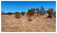
Open bushNatural tall woody vegetation communities, with canopy cover ranging between 10% and 35% and canopy heights exceeding 2.5 m. They are typically represented by open bush and woodland communities.
Remotesensing 15 05520 i002
GrasslandNatural grasslandNatural and semi-natural indigenous grasslands typically lack significant tree or bush cover, and the grassland component is dominant over adjacent exposed bare ground. Generally representative of low, grass-dominated vegetation communities in the Grassland and Savanna Biomes.
Remotesensing 15 05520 i003
BareBare ground/rock outcropSemi-natural or man-created non-vegetated areas. It is typically associated with permanent or near permanent bare ground sites that have insufficient spatial or temporal characteristics to be otherwise classified.
Remotesensing 15 05520 i004

2.2.2. XGBRFClassifier

Random Forest is an ensemble technique constructed by combining many decision trees. One such ensemble technique that underpins this study is the Extreme Gradient Boosting (XGBoost) technique, which implements gradient tree boosting decision tree algorithms where a predictive solution is achieved by simplifying the problem objectively and reducing the number of iterations to obtain an optimised solution [55]. XGBoost, also known as gradient boosting, multiple additive regression trees, stochastic gradient boosting, or gradient boosting machines, consists of an ensemble technique called Boost, in which errors made by existing models are corrected by the sequential addition of new models until there is no further improvement [100], according to Brownlee [87], boosting aims to determine whether a weak learner could be modified in order to improve the model. The first known accomplishment of boosting was through the application of adaptive boosting, where the vulnerable learners in the algorithm were the decision trees with a single split, also known as decision stumps. In recent years, adaptive boosting and related algorithms have been remodelled in statistical frameworks and are now known as gradient-boosting machines [87]. These new models cast boosting as a numerical optimisation problem where the objective is to add weak learners to a model and use a gradient descent procedure to minimise loss by the model [87]. Predictions of the residuals of prior models are summed up to make the final prediction in an approach that involves three elements: loss function optimisation, weak learner prediction, and additive model to vulnerable learners to minimise the loss function called Gradient Boost [87,100].
In recent years, XGBoost has become a de facto choice of ensemble methods [86] and has been proven to provide fast, state-of-the-art results and to act as a standard classification yardstick in many classification and regression scenarios [56,57]; it is more potent than the original Random Forest [87]. The success of the XGBoost classifier is bolstered by its ability to be scalable in all methods, resulting in systems being ten times faster than existing popular solutions [57,101,102]. It has algorithmic optimisation capabilities resulting in parallel and distributed computing power that enables quicker model exploration [57]. It can exploit out-of-core computation that allows a hundred million data to be processed on a desktop computer [57,102]. Lastly, the ensemble provides an end-to-end system that scales extensive data with a minimum number of clusters [57]. The XGBRFClassifier was selected for LC classification because of its computation efficiency and classification effectiveness compared to the conventional LC per pixel parametric and non-parametric classifiers, and because it is a relatively new machine-learning algorithm [57]. Its difference from other machine-learning algorithms is attributed to its computational proficiency, which is bolstered by algorithmic optimisation that enables it to simultaneously synchronise the objective function, loss function, and regularisation of the model complexity, enabling parallel computing and computational speed [50,56,57,87,100,101]. So far, new opportunities for studying temporal LC changes that affect land degradation have been created by integrating XGBoost, Random Forest, and fragmentation analysis [50,54,57,102].
Implementing the XGBoost classifier involved coding the algorithm in GEE and tuning hyperparameters. Model training and validation parameters were 70/30, training and testing. These parameters were adopted from a successful study, ‘Evaluation of light gradient boosted machine-learning technique in large scale land use and land cover classification’ [50]. In the GEE algorithm, Bands SRB1 (Blue), RSB2 (Green), and SRB3 (Red) for 1990–2009 and SRB2 (Blue), SRB3 (Green), and SRB4 (Red) for 2015 to 2020 were used for image classification. In the XGBRFClassifier, it is paramount to explore various hyperparameter configurations to find the best configuration that yields the best performance, and it is not easy to obtain the optimal one [101,103]. Hyperparameter tuning is essential for shaping the model architecture to achieve high precision and accuracy. This study employed the built-in code in the GEE environment ‘ee.Classifier.smileGradientTreeBoost’ to search for the best hyperparameter configurations (see Table 2). Changing this hyperparameter did improve the overall accuracy of the classifications.

2.2.3. Naïve Bayes

The concept of Bayes’ theorem, based on Naïve Bayes, was developed by the Reverend Thomas Bayes in the 18th century (precisely, in the 1700s) [60,91]. The “naïve” variant of Bayes’ theorem, which assumes conditional independence among features, was later introduced and popularised in machine learning and statistics [104]. The parametric classification algorithm gained prominence in the mid-20th century, particularly in natural language processing and text classification [105]. Naïve Bayes is simple to implement, computationally efficient, and particularly fast when dealing with high-dimensional data [91,105]. Its disadvantage is that it assumes feature independence, which can be a limitation in cases where features are dependent. It can be sensitive to noisy or irrelevant features and may not perform as well on more complex datasets [105]. Its advantages are that it can perform well when the naïve independence assumption is reasonably valid, such as in text classification tasks, is computationally efficient, and scales well to large datasets. Typically, it has fewer hyperparameters to tune, making it easier to use “out of the box” [91,104,105]. Implementing the Naïve Bayes classifier involved coding the algorithm in GEE and tuning hyperparameters. Model training and validation parameters were 70/30, training and testing. These parameters were the same as for the XGBRFClassifier; SRB2 (Blue), SRB3 (Green), and SRB4 (Red) for 2020 were used for image classification. The only hyperparameter to be tuned was lambda, which was set to 0.5.

2.2.4. Assessment of Classification Accuracy

It is prudent that before using the classification maps as decision-making tools, an essential step is to assess how effectively the pixels using the classification algorithm are sampled into the correct LC classes [70,106]. The accuracy assessment is a fundamental concept necessary to address reliability issues on the mapped changes corresponding to the actual change areas. It quantitatively evaluates the suitability of maps for the intended application [107]. Generally, by comparing the three accuracies, UA, PA, overall accuracies, and F1-score, researchers can select the most suitable algorithm for a given classification problem. We used the comparison of Naïve Bayes and the XGBRFClassifier to set a baseline performance for our task. We used the 2020 dataset for the comparison as it was the more recent dataset and compares well with ambient landscape configurations and could also be validated by ground truthing. Bayes is a simple and often fast algorithm that can serve as a benchmark. If XGBoost does not significantly outperform Naïve Bayes, it might not be worth the additional complexity, which requires more resources. This study used classified image data from 1990 as the benchmark for analysis of the preceding years. The Confusion Matrix generated by the GEE codes for the training data and the test data was used for the LULC accuracy assessment. The three accuracies, the UA, the PA, the overall accuracy, and the Kappa index were automatically computed using the codes. These two accuracies were, in turn, used to determine the F-score, a pixel-based accuracy assessment of the classifying algorithm; it shows the goodness of the classifier in the context of the PAs and UAs [70].
F s c o r e = 2 P A R A P A + R A
The F-score percentage deviation was calculated for the corresponding classes in the study years to assess the classifier’s accuracy over the study years.

2.2.5. Ground Truthing Sampling Techniques and Field Surveys

Stratified random sampling within the Cradle Nature Reserve was applied to collect field data using a Garmin eTrex 20 handheld GPS. This probability sampling technique, which divides the population into smaller groups with shared characteristics, was ideal for the already defined subgroups (strata) or areas of uniform thematic composition [108]. The number of random samples in each LULC was proportional to the total area covered by each stratum according to the Random Forest classification of 2020. The Random Forest classification raster data (tif map) had to be polygonised (raster-to-vector conversion) and the geometry fixed (fixed geometries) in the QGIS plugin. The fixed geometries belonging to the same class were then combined (that is, dissolved) into Random Forest classes for 2020. Using the analysis tool, the sampling points inside the polygons (classes) were generated (random points inside polygons) [109,110,111]. These points were then converted to WGS 84 coordinates for use in the field for surveying ground-truthing and accuracy assessment data.
The targeted points were located using the cardinal direction (N–S or E–W). Point attribute data were collected according to the predefined classification criteria for each surveyed or stacked point. In areas where this survey method fails due to the rugged terrain, natural topography, and drainages, Google Earth images from May 2020 were used to assist in populating the ground truthing data.

2.2.6. The Landscape Metrics

Landscape metrics underpin the study of natural forest fragmentation; they provide numerical information and temporal analysis of the landscape composition, configuration, and dimensions [7]. Fragmentation metrics at the patch, class, and landscape levels for the different LULC classes were performed using Landscape Ecology Statistics (LecoS), the QGIS python plugin [34,45,111]. LecoS has the function for calculating metrics on raster and vector data layers based on metrics derived from FRAGSTATS software ((integrated into QGIS through LecoS version 3.0.1)) and is embedded with functions to manipulate classified raster images [111]. FRAGSTATS software (integrated into QGIS through LecoS version 3.0.1) is well known for its detailed spatial and summary statistics that quantitatively describe patterns at patch, class, and landscape levels [45]. According to Matsushita and two other authors [112], although FRAGSTATS can calculate more than 100 landscape metrics, most metrics are highly correlated. The following metrics adapted from [5,7,113] are effective in evaluating forest cover changes using remote sensing data and were used in this study:
(a)
Total landscape area (ha) (TA): useful for landscape fragmentation analysis. It is the sum of the area of all patches in the landscape. TA increases without limit as the size of the landscape increases.
(b)
Percentage of Landscape (PLAND): useful for class-level fragmentation analysis. PLAND approaches zero as the proportional class area decreases, and if one patch is present, then PLAND will equal 100.
(c)
Largest patch index (LPI): determines the area of the most extensive patch in each class, expressed as a percentage of total landscape area, useful for landscape and class-level fragmentation analysis. LPI is a measure of dominance; as the value approaches zero, the largest patch becomes smaller; an LPI of 100 indicates that one patch is present.
(d)
The number of patches (NP): indicates the total number of patches. It is helpful for landscape and class-level fragmentation analysis. For a single patch, NP equals one, and the NPs increase as NP increases unlimitedly, the more fragmented the landscape.
(e)
Patch density (PD): indicates the number of patches per unit area. It is useful for landscape and class-level fragmentation analysis. Higher PD indicates a highly fragmented landscape.
(f)
Mean patch size (MPS): provides the average patch size for the class in hectares. It is useful for landscape and class-level fragmentation analysis. A small MPS implies a highly fragmented landscape.
(g)
Patch cohesion index (COHESION): provides valuable information for class-level connectivity analysis. COHESION approaches zero as the patches become more isolated, and higher values indicate more aggregated patches.
(h)
Shannon’s diversity index (SHDI): provides valuable information for landscape-level heterogeneity analysis. Its value ranges from 0 to 1; it approaches 0 as the landscape is dominated by one LC type or less diversity. It approaches one as the LC types become roughly equal, implying a more diversified landscape.
From the listed metrics, the study derived the hypothesis testing of the landscape metrics; see Table 3. Hypothesis testing of landscape metrics is essential to landscape ecology and spatial analysis [114,115]. Landscape metrics provide quantitative measures of landscape patterns and spatial characteristics, and hypothesis testing allows researchers to draw meaningful conclusions about the ecological processes and phenomena driving these patterns [114,115]. It enables researchers to explore ecological questions, compare landscapes, detect changes over time, and make informed decisions about land management and conservation strategies based on objective and statistically sound evidence [115].

2.2.7. Land Use/Land Cover Changes

The LULCC detection was carried out using the QGIS plugin SCP postprocessing LC change tool for 1990–1998, 1998–2009, 2009–2015, 2015–2020, and 1990–2020. The input data for this process were the landscape classification maps/tagged image file (tif) produced using the XGBRFClassifier. The classification nomenclature was identical (number and sequence of LULC Macroclasses and classes) for all the years to generate harmonised geometric and thematic content [49]. Maps showing the transition of landscape patches within the time frames were developed to depict the changes.

3. Results

3.1. Comparison of Accuracy Assessment of Classification Algorithms Using 2020 Dataset

Table 4 show the comparison of the three accuracies, UA, PA, overall accuracies, and F1-score for the 2020 data. As already stated in Section 2.2.4, if XGBoost accuracies and F1-score do not significantly outperform Naïve Bayes, as demonstrated in our study, see Table 3, it might not be worth the additional complexity, which requires more resources. However, in this study, we were not resource-constrained. We elected to use the XGBRFClassifier after assessing the comparison results in Table 4 instead of Naïve Bayes, which is generally less resource-intensive and saves computational resources and time [60]. The following reasons motivated our selection:
  • Future Proofing: Even if the XGBRFClassifier does not significantly outperform Naïve Bayes on our current dataset, it may be more adaptable to future changes in data distribution or feature sets [116]. Naïve Bayes is relatively simple and may not handle data shifts or feature additions as gracefully as the XGBRFClassifier [117].
  • Continuous Model Improvement: In machine-learning competitions and real-world applications, practitioners often use a variety of algorithms, including the XGBRFClassifier, to continually improve model performance. The XGBRFClassifier can be an essential tool in this iterative process [116].
  • Advanced Techniques: The XGBRFClassifier supports advanced techniques such as gradient boosting, early stopping, and custom loss functions, which can be leveraged to improve performance in specific scenarios [116,118].
  • Scalability: The XGBRFClassifier is designed to scale efficiently to large datasets, making it suitable for situations where there is a large amount of data that Naïve Bayes may struggle to handle effectively [116,117,118].
  • Transferability: In future, if we plan to apply our model to different datasets or similar classification tasks, the XGBRFClassifier might offer better transferability [116]. It can adapt to varying data distributions and capture different patterns effectively [117].
  • Hyperparameter Tuning: The XGBRFClassifier offers more hyperparameter tuning options and flexibility compared to Naïve Bayes [117]. If we have the resources and time to perform thorough hyperparameter tuning, we may be able to fine-tune the XGBRFClassifier to achieve better performance than the current results [116,117].

3.2. Ground Truthing Accuracy Assessment

Data collected by the field visit could not sufficiently cover the study area owing to inaccessibility challenges outlined in Section 2.2.5. Despite the challenges, 120 data points were surveyed, distributed as 30, 35, 28, and 27 for Indigenous forest, Open bush, Natural grass, and Bare ground/rock outcrop, respectively. The confusion matrix derivatives (see Table 5) and benchmark accuracy assessment from the Naïve Bayes algorithm are high enough to confirm the usability of the classified maps for future LULC assessments of the Cradle Nature Reserve.

3.3. Accuracy Assessment and Land Cover Digital Classification of Study Area (1990–2020)

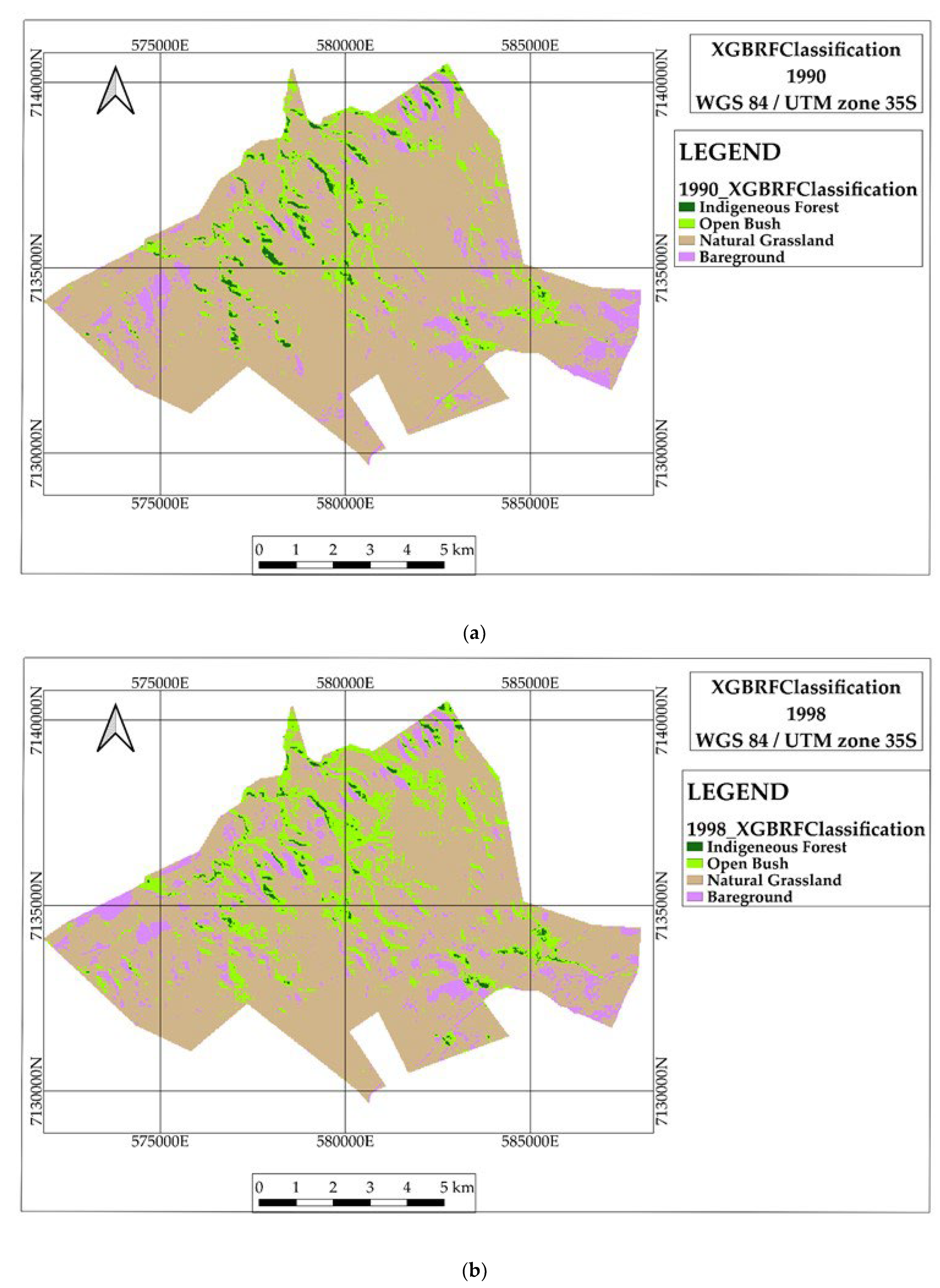
Figure 3a–e shows the XGBRFClassifier classified images. The UA, PA, overall accuracy, Kappa index, and F1 score are shown in Table 5 and Table 6 using a 70/30 training/testing evaluation model. An inspection of Table 5 and Table 6 shows that the overall accuracy, Kappa coefficient, and F-score are sufficiently high for the onward use of the classified maps. Indigenous forest and open bush overall accuracies are generally lower than the rest because of the difficulty distinguishing them during the training data preparation.

3.4. Land Use/Land Cover Spatial Temporal Change Detection

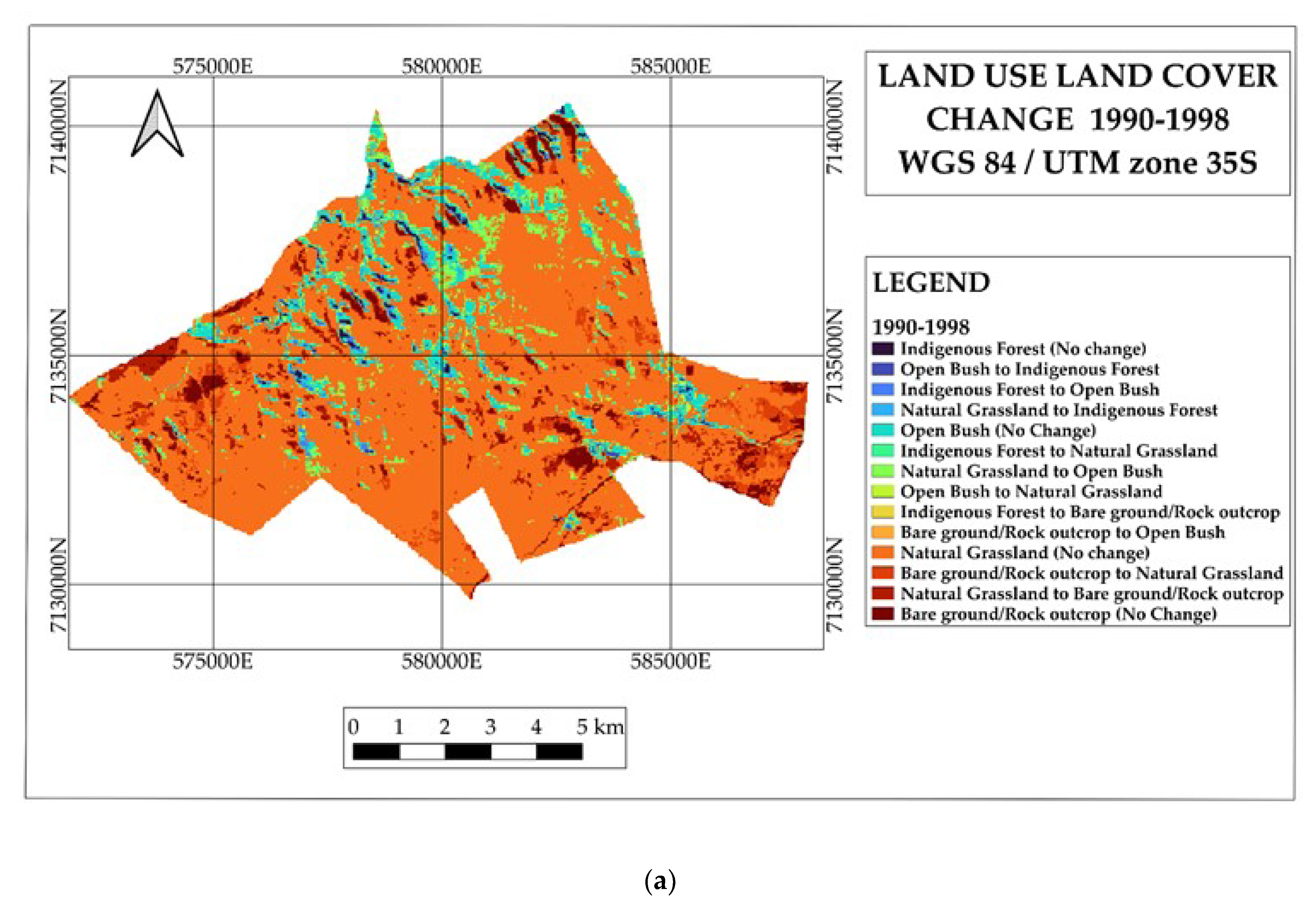
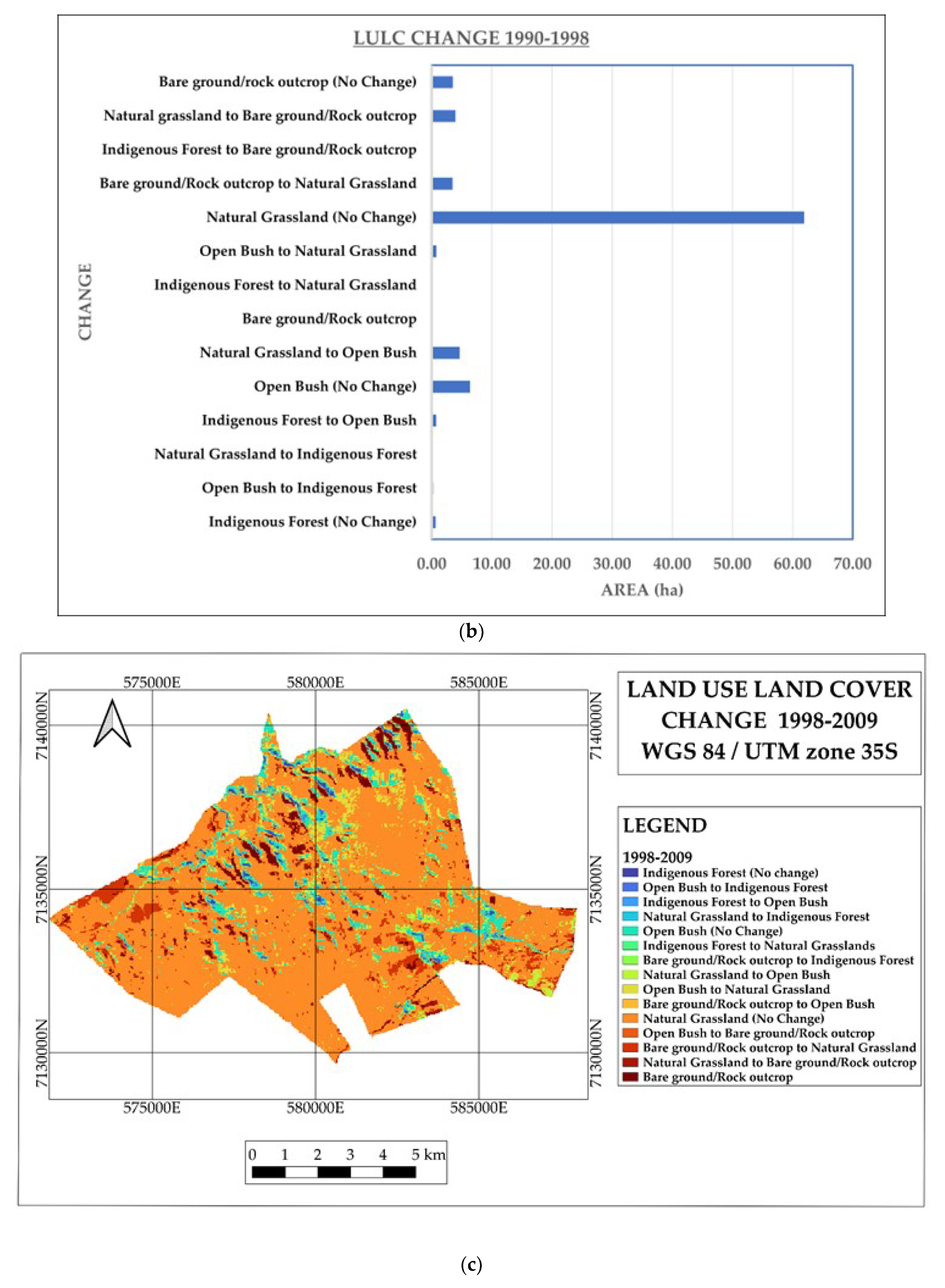
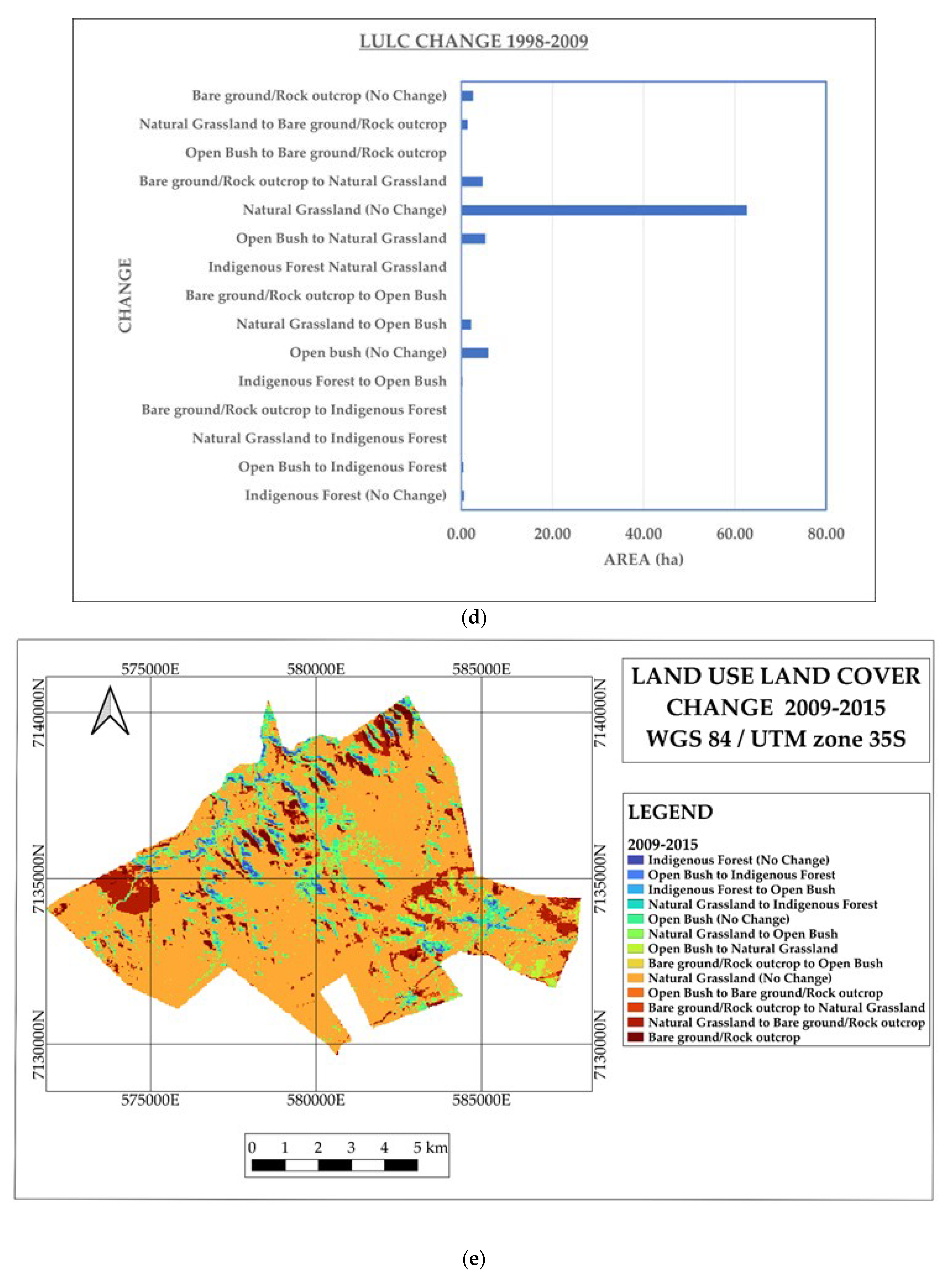
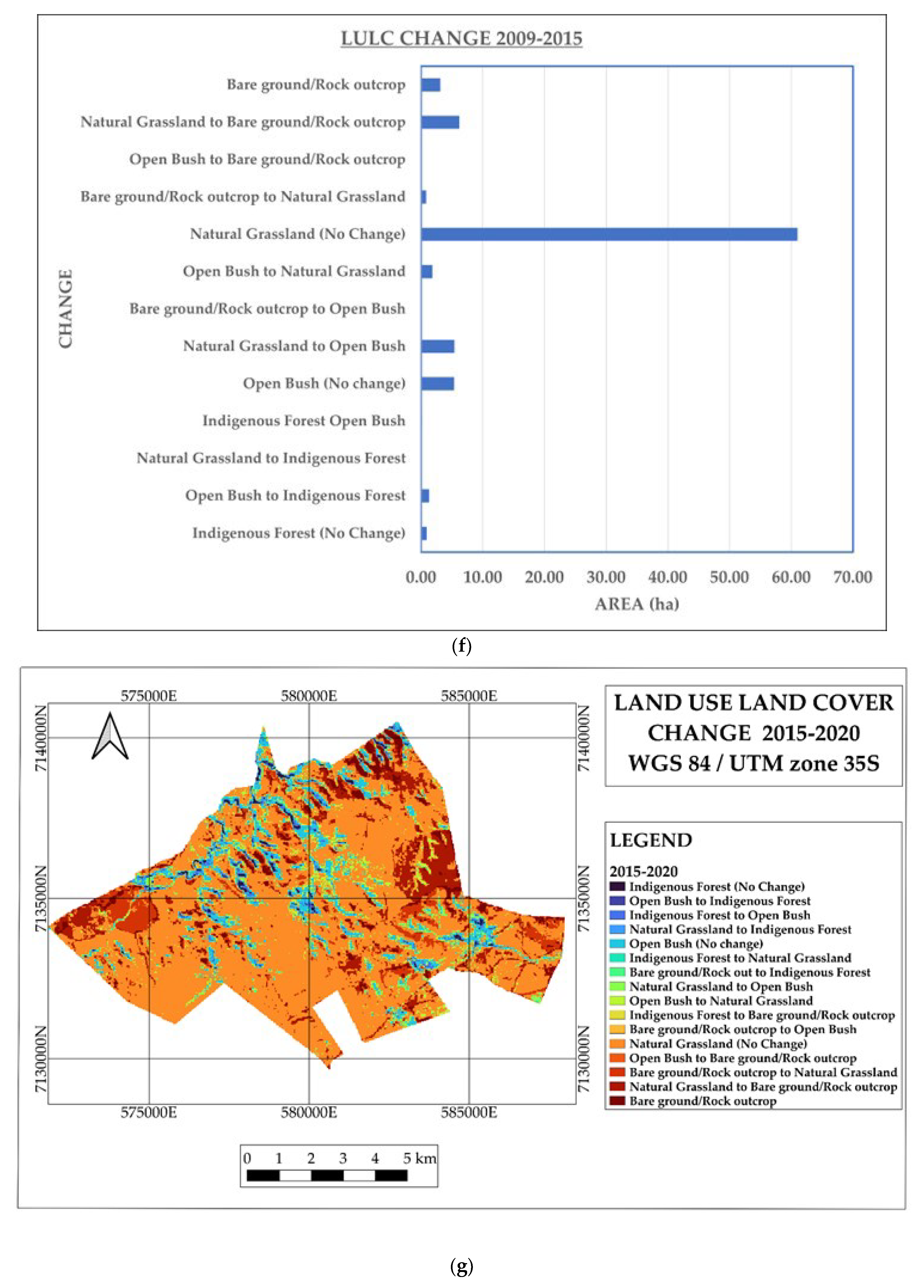
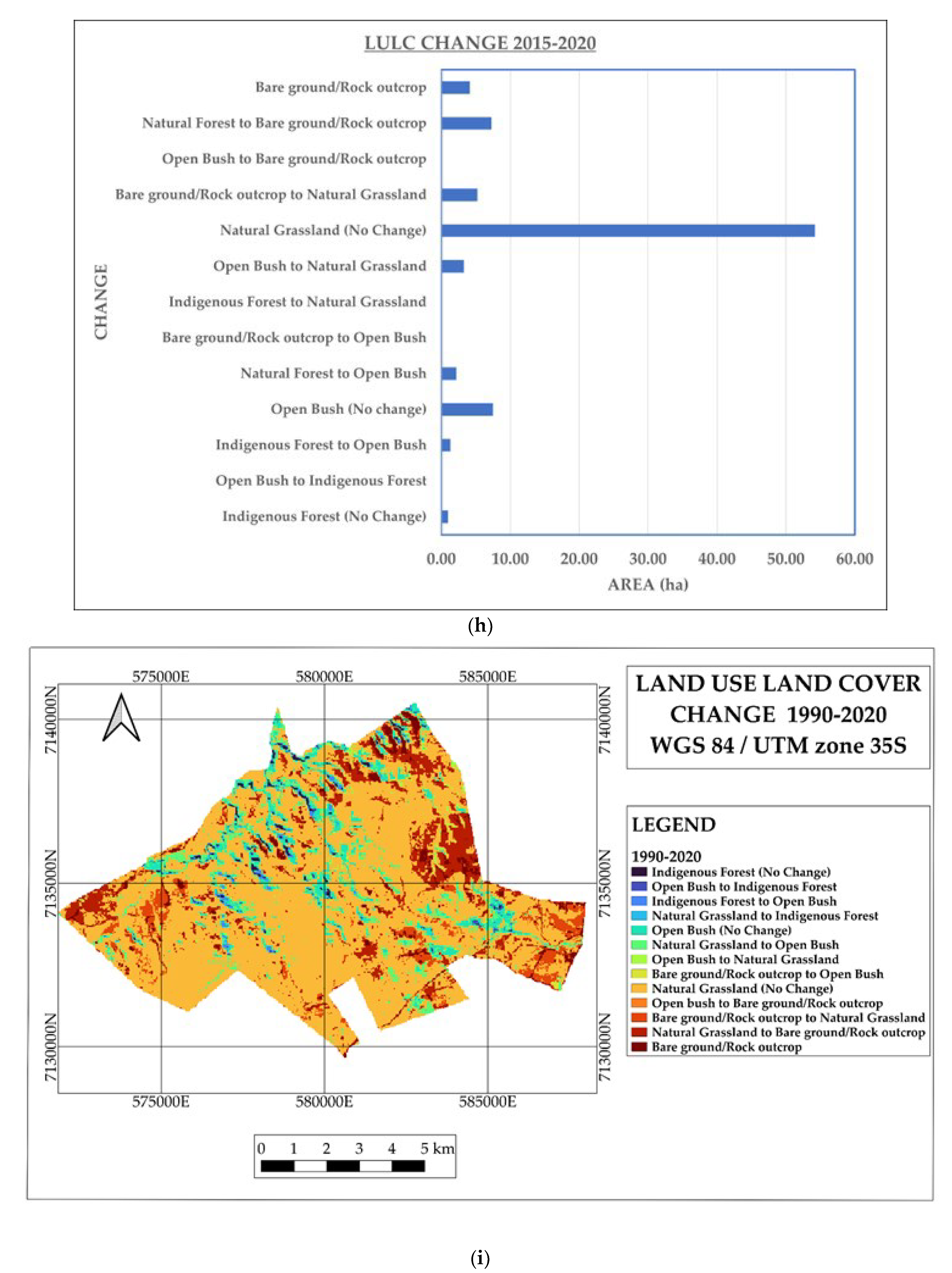
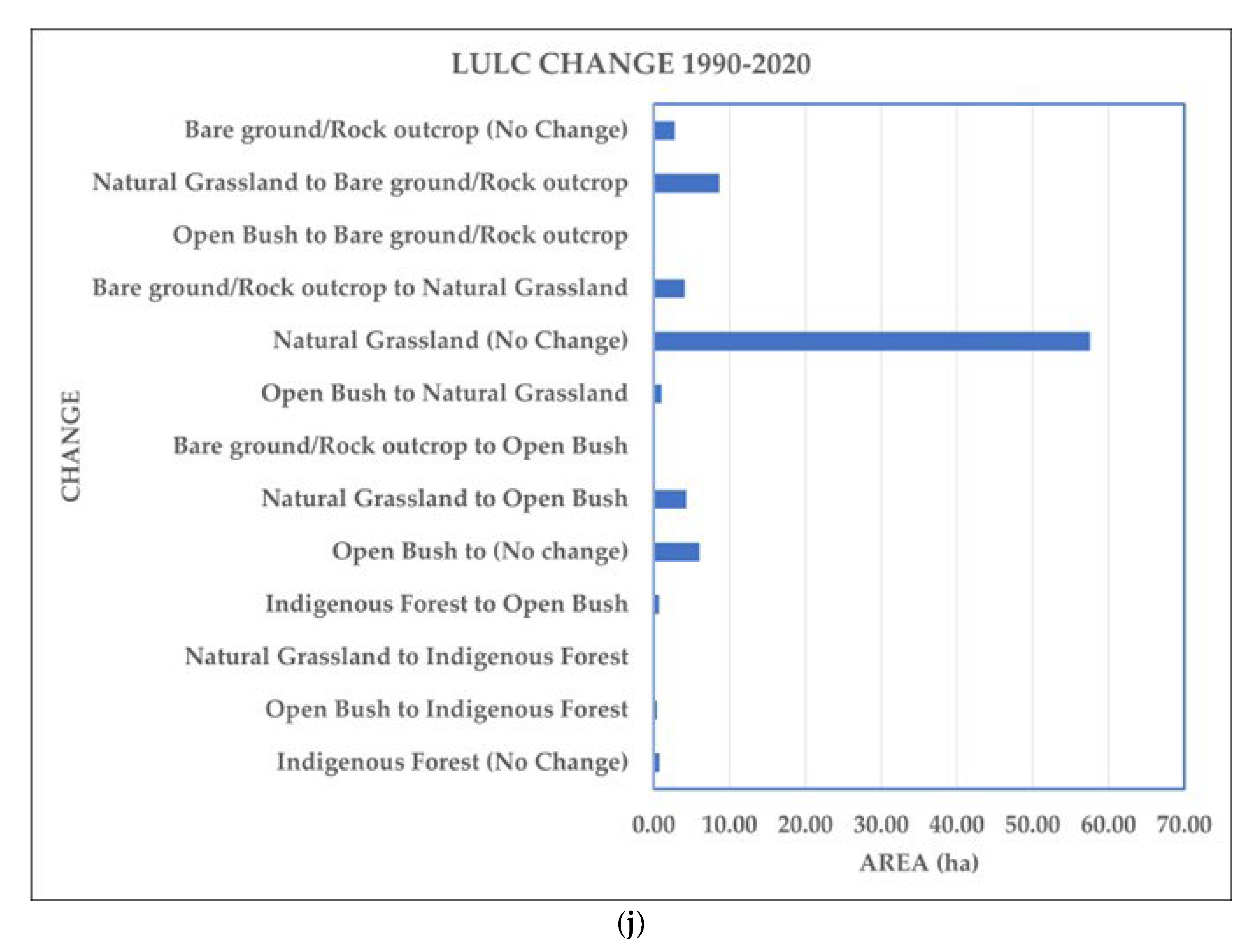
The LULC variations in the study area, 8624.77 hectares throughout the study period (1990–2020), are presented in Figure 4a–j. It can be deduced from Table 7 that, over the three decades, the area covered by bare ground/rock outcrop increased significantly. In 1990–1998, the landscape dominated by indigenous forest lost 45.41 hectares, open bush gained 431.76 hectares, natural grassland lost 436.93 hectares, and bare ground/rock outcrop gained 50.58 hectares. From 1998 to 2009, the landscape dominated by indigenous forest gained 15.27 hectares, open bush lost 312.83 hectares, natural grassland gained 647.16 hectares, and bare ground/rock outcrop lost 349.60 hectares. From 2009 to 2015, the landscape dominated by indigenous forest lost 120.30 hectares, open bush gained 233.66 hectares, natural grassland lost 896.09 hectares, and bare ground/rock outcrop gained 542.13 hectares. Between 2015 and 2020, landscape dominated by indigenous forest lost 118.93 hectares, open bush lost 6.87 hectares, natural grassland lost 93.80 hectares, and bare ground/rock outcrop gained 205.86 hectares. Over the 1990–2020 period, landscape dominated by indigenous forest lost 28.76 hectares, open bush acquired 359.45 hectares, natural grassland lost 779.66 hectares, and bare ground/rock outcrop acquired 448.97 hectares.

3.5. The Landscape Metrics and Dynamics: Class Level

The total landscape areas (TA) (see Table 8) do not depict a straightforward pattern from one study year to another. However, over the three decades, 1990–2020, from the LULC temporal change detection matrices (see Table 7), it can be deduced that the landscape dominated by indigenous forest lost 28.76 hectares (0.34%), open bush gained 359.45 hectares (4.23%), natural grassland lost 779.66 hectares (9.18%), and bare ground/rock outcrop gained 448.97 hectares (5.29%). The LPI for natural grassland (see Table 8) is significantly more than other landscape classes in the study area, indicating the dominance of grassland in the Cradle Nature Reserve. This agrees with the landscape description of the study area given by [84]. In addition, it can be deduced from Table 8 that the MPS decreased by 44% from 77.19 hectares in 1990 to 43.14 hectares in 2020 for natural grassland, indicating an increased fragmentation in the class.
The NP increased by 11% during the 1990–2020 period, indicating a more fragmented landscape in 2020 than in 1990 (see Table 8). There was a gradual increase in the number of patches from 1990 to 1998 (5%), 1998 to 2009 (23%), and 2009 to 2015 (22%), and a significant drop in number of patches from 2015 to 2020 (29%); however, the overall increase in the number of patches indicates a more fragmented landscape in 2020. A substantial change in the open bush density in the patches from 1990 to 2020 (4.72 to 9.49) indicates that the class was significantly fragmented over the three decades. The PD for natural grassland and indigenous forest shows a marginal increment of 1.06 to 2.44 and 1.94 to 3.56, respectively, indicating increased landscape fragmentation in these classes (see Table 8). Bare ground/rock outcrop PD dropped from 5.39 to 5.15 over the three decades, implying consolidation of the patches and a decrease in class fragmentation.
COHESION did not change significantly over the study period (see Table 8). None of the index values approaches zero, indicating that the patches are not isolated and that the landscape patches did not become aggregated over the study period. The SHDI from 1990 to 2020 increased from 0.65 to 0.82, although it dipped to 0.57 in 2009 (see Table 8). Generally, the trend indicates a loss of dominance by one LC class. This trend confirms the dominance of natural grassland in the landscape, as depicted in the XGBRFClassification for 1990 to 2020 (see Figure 4a–j). However, the increase in SHDI confirms the loss of dominance of natural grassland owing to a noticeable gain in the LC by the open bush and bare ground/rock outcrop LCs [119,120,121,122].

4. Discussion

4.1. Comparison of Naïve Bayes and Gradient Boosting Random Forest Classifiers

The XGBRFClassifier successfully classified land cover and land use in the Cradle Nature Reserve from 1990 to 2020. The ensemble classifier performed well for PA, UA, overall accuracies, Kappa index, and F-score when compared with Naïve Bayes and previous studies by Alam et al. (2020), Rwanga and Ndambuki (2017), Kavzoglu and Teke (2022), and Britz (2022) [46,48,55,106]. The classification results are shown in Figure 3a–e, and periodic changes in 1990–1998, 1998–2009, 2009–2015, and 2015–2020 are shown in Figure 4a–j. From 1990–2020 (see Figure 4i–j), 29 hectares of indigenous forest were converted to other landscape classes, mostly into open bush. Three hundred fifty-nine hectares changed from indigenous forest and natural grassland to open bush. A significant hectarage of the natural grassland (780 hectares) was lost to other landscape classes, mainly to bare ground/rock outcrop and, to a lesser extent, open bush. Bare ground/rock outcrop grew significantly by 449 hectares over the years, mainly due to the natural grassland’s disappearance. Over the 30 years, some areas may have reverted to tree/bush cover in the natural grassland landscape, or inter-annual seasonal differences could account for the changes.
In recent years, XGBoost has acted as a standard classification yardstick in many classification and regression scenarios [56,57], and it is more powerful than the original Random Forest [87]. In recent studies, the ensemble of XGBoost and Random Forest (XGBRFClassifier) has been considered as having superior capabilities in dealing with real-world problems, such as in mapping landslide-susceptible areas in Macka County, situated in Trabzon Province, Turkey [55], and in Dazhou town, located in Wanzhou District, China [123], and in mapping areas suspectable to flooding by the Spercheios river, Greece [124], and the Bâsca Chiojdului River Basin in Romania [125]. In all scenarios, the ensemble demonstrated its capabilities in capturing intricate patterns in fragmented landscapes, which exhibit complex and nonlinear relationships between various landscape features and their classes, resonating well with the karst terrain in the Cradle Nature Reserve. The ensemble found its station in predicting suspectable landslide and flood areas; in this study, areas suspectable to alien species invasion were informed by the increasing presence of bare ground. As established in these noted examples, the choice of the ensemble is buttressed by its robustness in the presence of irrelevant features, as it assigns low importance to them during the feature selection process, avoiding overfitting with limited landscape data, as is the case in the Cradle Nature Reserve, and demonstrates flexibility to hyperparameter tuning, which was also employed in this study to optimise the performance in classifying the Cradle Nature Reserve landscape.
This study used the family of Kappa indices to accurately assess the land cover classification. While the Kappa indices remain the most widely used accuracy assessment indices in remote sensing land cover classification, researchers have highlighted the shortcomings of the Kappa indices. Pontius and Millones [126] emphasise that the Kappa indices have flaws and recommend the use of quantity disagreement and allocation disagreement parameters. Olofsson and five other authors [107] provide good practice recommendations for accuracy assessment and area estimation by focusing the procedure for accuracy assessment on sampling design, response design, and analysis. In contrast to Pontius and Millones [126], who announced the demise of the Kappa indices, Olofsson and five other authors [107] provided a more balanced approach that embraced acceptable practices that yielded scientifically credible results, such as the Kappa indices. Notwithstanding its shortcomings, the Kappa indices remain the most widely used accuracy assessment indices, despite the emergence of more novel indices.
The sampling technique used in this study was stratified random sampling. Although it is considered effective in reducing bias, it has issues even if adequately implemented. The vegetation in the Cradle Nature Reserve is seasonal and subjected to burning regimes; depending on the time of the year, some strata must be better defined, and the sampling technique suffers from selection biases. Some areas that could have been covered by natural grass might appear to be bare ground for the natural grasslands’ classification, even though the grass will grow later in the rainy season. In addition, even with the implementation of correct sampling procedures, measurement biases still occur. The karst terrain of the nature reserve resulted in some random samples being placed in geographically inaccessible areas, such as in the middle of flowing streams and on top of mountains with rugged terrain to climb. For this reason, ground truthing these areas relied on Google Earth images, and the result could have been different if these places were physically visited.

4.2. Land Use and Land Cover Changes from 1990 to 2020

It was noted that the Cradle Nature Reserve was previously farmland [85] used for pastures and crop farming; the change in LU following the conversion of the land to a nature reserve may have contributed to the significant transformation of the landscape from natural grassland to other landscape classes. The depletion of the indigenous forest versus gain by open bush could be attributed to the introduction of herbivores, including buffalo, giraffe, and wildebeest, which survive by eating the branches of the indigenous forest. The decrease in grassland could also be attributed to the worldwide phenomenon of climate change; studies have established that climate change results in high rates of land degradation from enhanced desertification and nutrient-deficient soils [127]. Overgrazing could also have opened the natural grassland to invasive species growth and conversion of the landscape to bare ground/rock outcrop class.
The opportunities for recycling nutrients and the movement of resources around landscapes are hampered by the scarcity or disappearance of long-lived plants [128]. Soil surface conditions, water redistribution on the soil surface, and landscape functionality are exhibited by patchy vegetation patterns owing to reduced plant cover [129]. Consequently, the degradation of the original plant cover is primarily attributed by many scholars to anthropogenic disturbances and climatic fluctuations [75]. Similarly, the land degradation and ecological succession witnessed in this Cradle Nature Reserve landscape study can be attributed to temporal LC changes driven by anthropogenic and climate conditions [130]. Abiotic stress factors such as natural phenomena such as drought, floods, and global warming contribute to landscape fragmentation that negatively impacts LC and geomorphological processes [16,112,130,131]. The landscape variability can be attributed to consolidating different farms with different land use and ecosystem functionality [85]. Biotic factors such as animal grazing patterns impact the LC dynamics in the nature reserve [16,130,131]. The introduction of wild game species during the establishment of the Cradle Nature Reserve and the conversion of previous farmlands to game reserves is likely to have been a significant source of anthropogenic-driven changes in the landscape [83]. It implies an induced redistribution, dispersion, and changes in the area’s diversity of flora and fauna [39,72,103,112]. Grazing patterns, for instance, affect the vegetation cover’s structure and composition, critical in protecting the landscape from soil erosion, a driving force in land degradation [132,133]. As already discussed, the invasion of grasslands by shrubs and alien invasive plants such as the pompom weed often results in a semiarid environment characterised by a vegetation pattern that combines vegetated and bare patches with various spatial characteristics [134,135,136,137]. Land fragmentation can be viewed as a cause and a consequence of LU change [5,7,39,45,49]. In the Cradle Nature Reserve context, it is fair to say that the introduction of wild game species, the shift from agricultural lands to natural grasslands, and the spread of invasive alien species have contributed to the current land fragmentation.
This study has established that the Cradle Nature Reserve landscape becomes more fragmented as the natural grasslands are converted to bare ground/rock outcrop. The pervasive nature of invasive alien plant species on the rangelands is detrimental to the growth of native vegetation. It has been established that invasive plants reduce grass cover and increase in response to disturbances such as the burning regimes in the grasslands, as in the Cradle Nature Reserve case [73,77]. Bare ground/rock outcrop increases exposure to soil erosion. Guided by these findings from the study, it is recommended that speedy eradication of invasive alien plants (especially pompom weed) needs to be carried out; this should be done to preserve the grasslands that provide food for the thriving nature reserve and maintain the source of information for documenting hominin dietary ecologies. Preserving the Cradle Nature Reserve is also critical in maintaining the rangelands, thus supporting game farming and COH tourism. It is also suggested that the Cradle Nature Reserve environmental managers should revisit their burning regimes to align with initiatives for eradicating invasive species, including the pompom weed.

4.3. Landscape Structural Changes due to Fragmentation

Global trends of habitat fragmentation versus spatial patterns in the Cradle Nature Reserve can be determined by analysing the landscape fragmentation in the nature reserve over the last three decades [138]. From 1990 to 2015, the total number of patches in the nature reserve generally increased, as shown in Table 8, although by 2020 there was a significant drop in patch numbers. Landscape fragmentation also slowed down from 2015 to 2020 for the other landscape classes. Importantly (as noted in other studies of LC change at the national level and Gauteng province in which the Cradle Nature Reserve is situated), this mirrored the trend for the rest of the country from 1990 to 2020. These studies noted a general increase in land fragmentation due to increased human population and residential development, pressure from industrial expansion, and alien species invading natural grassland [44,45,73,99,106,139,140,141].
In the study area, the conversion of the farms to the nature reserve could have accelerated the fragmentation of the landscape from 1990 to 2015 and may have slowed down from 2015 to 2020 owing to management interventions; the latter may have allowed the vegetation of the nature reserve to recover naturally. Limiting the numbers and types of game species based on vegetation monitoring and adherence to controlled veld burning regimes was implemented by the nature reserve management [L. Berger and W. Maduwa, personal communication during site visit, 15 February 2023]. Shannon’s diversity and COHESION values did not indicate significant changes in LC, except for in 2009, when the value was significantly low (0.57). However, the overall trend from 1990 to 2020 reflects the dominance of natural grassland, which resonates well with the game species present in the nature reserve.
As noted by [142], the shift from analysing the spatial heterogeneity of ecological systems using static frames to dynamic frameworks has been made possible by the advent of fragmentation analysis techniques. These techniques have greatly expanded the influential capabilities of remote sensing-based research [142]. Fragmentation metrics in managing nature reserves and agricultural ecosystems share some similarities. Fragmentation metrics in both circumstances help management understand how changes in the arrangement and connectivity of landscapes impact ecosystem services and subsequently influence land use decisions [45,142]. In both cases, fragmentation often results in smaller isolated fields or patches that result in the loss of natural habitat and increased edge effects, ultimately declining the biodiversity and the landscape capacity to support ecosystem services [142,143,144,145]. Studies with similar themes have established that anthropogenic factors are significant players in the increase of landscape fragmentation. Some of these studies’ themes include land use changes due to urbanisation and change in landscape pattern [143], landscape fragmentation and analysis of LULC [142], essential fragmentation metrics for agricultural policies [144], and landscape pattern analysis and ecological network planning [145], whose findings resonate well with the revelations from this study. Anthropogenic factors such as tourism development (road networks and infrastructure development), land tenure and ownership issues (consolidation of farms and change of land use), and fire management practices (grass burning regimes) all contributed to the study area landscape fragmentation. These activities exposed the Cradle Nature Reserve to colonisation of parts of the landscape by invasive alien species such as the pompom weed. As established by other studies [141,146,147], the impact of the colonisation of the landscape by invasive alien species contributes to habitat alteration (transforming of original habitat structure), altered fire regimes (change of natural fire alters the composition and structure of vegetation), edge effects (reduce the quality of interior habitat), biological invasions (lead to shifts in vegetation patterns and ecosystem dynamics), corridor disruption (limit effectiveness of conduits for native species movement), predation and competition (disruption of food webs), spread mechanisms (introduction of new species to uninvaded areas), and hybridisation.
It is also possible that invasive trees/bushes have intruded into the natural grassland. Ecological studies are pursuing the impact of invasive species on the South African landscape [141]; studies have shown that this phenomenon seriously impacts biodiversity. While this study did not directly quantify the impact of invasive alien species on the Cradle Nature Reserve, the transformation of natural grasslands to bare ground/rock outcrop is a testament to the effect of invasive alien plants. Ground truthing surveys established that some invasive plants drastically reduce grass cover. Pompom weed has been sighted in the nature reserve [73,141,148] and could contribute to the natural grassland’s degradation, which is discussed further below.
Invasive alien plants are of concern in South Africa as they are known to invade disturbed areas and natural grasslands in South Africa [L. Berger and W. Maduwa, personal communication during site visit, 15 February 2023]. Our ground truthing surveys confirmed the widespread distribution of the pompom weed. This mirrors the pattern of the pompom weed currently invading the grassland and savanna biomes in the rest of South Africa; researchers further predict that this will continue spreading in the southern African sub-region [73,134,141,149]. The gradual landscape degradation owing to the invasion of grasslands and agricultural land by exotic plant species has been well studied and documented [73,134,135,146,150,151]. Among the studies, Valentin and two other authors [76] suggests two main hypotheses to elucidate the origins and development of vegetation and bare soil surface mosaics (also known as banded vegetation patterns) in arid areas. Specifically, this involves the gradual degradation of an initially uniform plant cover owing to climatic or human disturbances and the colonisation of previously degraded bare areas under improving climatic or land use conditions. Dunkerley and Brown [152], Bryan and Brun [153], and Lepron [154] have supported these hypotheses and have agreed on the point that rangeland deterioration resulted from the disruption of a formerly more continuous vegetation cover by overgrazing, trampling, and precipitation decline. For instance, abandoned fields in semiarid southeast Spain are reported by Cammeraat and Imeson [74] as having been colonised by Stipa tenacissima under drought and grazing pressure conditions.
The application of Extreme Gradient Boosting Random Forest and landscape metrics in studying land cover change within a protected archaeological area is relatively novel, and this study recommends that future studies should pay greater attention to land degradation induced by invasive plants within protected areas, particularly archaeological world heritage sites. In addition, studying land cover degradation in a heritage site, as in the Cradle Nature Reserve, has significant implications for preserving and managing the site’s cultural and natural values. Some of the implications are as follows:
  • Increasing fragmentation and decline in vegetation will ultimately reduce the grazing and browsing capacity of the nature reserve and the area’s game-carrying capacity. Loss of native vegetation species associated with paleo-diets also impacts archaeological studies in the world heritage site.
  • Unchecked land cover degradation has long-term ecological consequences because it disrupts the delicate balance of the natural environment within and around the nature reserve, including loss of habitat, biodiversity decline, soil erosion, and alteration of local ecosystems, which together diminish the aesthetic value of the heritage site and negatively impact its tourism value. Consequently, it destroys the crucial local economies and threatens sustainable tourism.
  • The results from the study are informative to the development and implementation of effective legal and policy frameworks for the Cradle Nature Reserve site management and conservation. It is hoped that the findings from the study highlight the need for more stringent regulations and enforcement measures to protect the reserve from invasive alien species such as the pompom weed.

5. Conclusions

Using satellite imagery, the XGBRFClassifier successfully classified the Cradle Nature Reserve landscape into four classes: indigenous forest, open bush, natural grassland, and bare ground/rock outcrop. This classification revealed LULCC trends in the landscape from 1990 to 2020, showing environmental degradation over this period. In addition, the landscape metrics derived from the classified images confirmed the ground-truthing findings, namely the dominance of the natural grassland class and the presence of the invasive pompom weed. The degradation of the dominant grassland class is evidenced by increased landscape fragmentation, as demonstrated by the increased number of landscape patches in 2020 (compared to 1990) in the natural grassland.
Over the 1990–2020 study period, the area covered by bare ground/rock outcrop increased significantly (448.97 hectares), representing 39% of the landscape cover change in bare ground/rock outcrop since 1990. The second-most significant change was the gain in open bush landscape cover (359.45 hectares), representing 32% of the landscape. Indigenous forest and natural grassland lost their share of the landscape cover in the Cradle Nature Reserve over the same period by 28.76 hectares (26%) and 779.66 hectares (12%), respectively. The loss was primarily to bare ground/rock outcrop. While these changes in the landscape cover are anticipated to occur naturally (because of the dynamic nature of the landscape), they are accelerated by anthropogenic factors. Such factors include the introduction of various species of game and invasive plants such as the pompom weed. The latter species is known to accelerate the degradation of environments and indigenous plant food sources associated with hominin diets. Therefore, it is prudent for Cradle Nature Reserve environment management to speed up processes or programmes to eradicate invasive alien plants.

Author Contributions

Conceptualisation, P.M. and C.M.; methodology, P.M. and C.M.; software, C.M.; validation, C.M.; formal analysis, C.M.; investigation, C.M.; writing—original draft preparation, C.M and P.M.; writing—review and editing, C.M and P.M.; visualization, C.M.; supervision, P.M. All authors have read and agreed to the published version of the manuscript.

Funding

This research was funded through a bursary by the Lee Burger Foundation. The A.P.C. was funded by GENIUS.

Data Availability Statement

Data are contained within the article.

Acknowledgments

We would like to thank Lee Burger for granting us access to the Cradle Nature Reserve and for providing logistical support.

Conflicts of Interest

The authors declare no conflict of interest.

References

  1. Martínez-Valderrama, J.; Ahmed, Z.; Gui, D. Oasification and Desertification under the Framework of Land Degradation Neutrality Chapter Invitation—”Symbiotic Association of Microorganisms with Medicinal and Herbal Plants” View Project Special Issue “Sustainable Approaches for Plant Conservation under Emerging Pollutants Volume II” Sustainability (Impact Factor = 3.889) View Project Oasification and Desertification under the Framework of Land Degradation Neutrality †. Environ. Sci. 2023, 25, 94. [Google Scholar] [CrossRef]
  2. Chasek, P.S. The Convention to Combat Desertification: Lessons Learned for Sustainable Development; Sage Publications Inc.: Thousand Oaks, CA, USA, 1997; Volume 6. [Google Scholar]
  3. Pricope, N.G.; Daldegan, G.A.; Zvoleff, A.; Mwenda, K.M.; Noon, M.; Lopez-Carr, D. Operationalizing an Integrative Socio-Ecological Framework in Support of Global Monitoring of Land Degradation. Land Degrad. Dev. 2023, 34, 109–124. [Google Scholar] [CrossRef]
  4. Ambalam, K. Challenges of Compliance with Multilateral Environmental Agreements: The Case of the United Nations Convention to Combat Desertification in Africa. J. Sustain. Dev. Stud. 2014, 5, 145–168. [Google Scholar]
  5. Adepoju, K.A.; Salami, A.T. Geospatial Assessment of Forest Fragmentation and Its Implications for Ecological Processes in Tropical Forests. J. Landsc. Ecol. 2017, 10, 19–34. [Google Scholar] [CrossRef]
  6. Kellndorfer, J. SAR for Mapping Deforestation and Forest Degradation. In The Synthetic Aperture Radar (SAR) Handbook: Comprehensive Methodologies for Forest Monitoring and Biomass Estimation; NTRS: Washington, DC, USA, 2019; pp. 41–57. [Google Scholar]
  7. Martinez del Castillo, E.; García-Martin, A.; Longares Aladrén, L.A.; de Luis, M. Evaluation of Forest Cover Change Using Remote Sensing Techniques and Landscape Metrics in Moncayo Natural Park (Spain). Appl. Geogr. 2015, 62, 247–255. [Google Scholar] [CrossRef]
  8. Maitima, J.M.; Mugatha, S.M.; Reid, R.S.; Gachimbi, L.N.; Majule, A.; Lyaruu, H.; Pomery, D.; Mathai, S.; Mugisha, S. The Linkages between Land Use Change, Land Degradation and Biodiversity across East Africa. Afr. J. Environ. Sci. Technol. 2009, 3, 310–325. [Google Scholar]
  9. Mitchell, A.L.; Rosenqvist, A.; Mora, B. Current Remote Sensing Approaches to Monitoring Forest Degradation in Support of Countries Measurement, Reporting and Verification (MRV) Systems for REDD+. Carbon Balance Manag. 2017, 12, 9. [Google Scholar] [CrossRef]
  10. Zekarias, T.; Gelaw, A. Impacts of Land Use/Land Cover Change on Wetland Ecosystem Services of Lake Abaya-Chamo Wetland, Rift Valley of Ethiopia. Geol. Ecol. Landsc. 2023, 1–12. [Google Scholar] [CrossRef]
  11. Raihan, A. The Dynamic Nexus between Economic Growth, Renewable Energy Use, Urbanization, Industrialization, Tourism, Agricultural Productivity, Forest Area, and Carbon Dioxide Emissions in the Philippines. Energy Nexus 2023, 9, 100180. [Google Scholar] [CrossRef]
  12. Shewit, G.; Minwyelet, M.; Tesfaye, M.; Lewoye, T.; Ferehiwot, M. Land Use Change and Its Drivers in Kurt Bahir Wetland, North-Western Ethiopia. Afr. J. Aquat. Sci. 2017, 42, 45–54. [Google Scholar] [CrossRef]
  13. Anh, N.T.; Nhan, N.T.; Schmalz, B.; Le Luu, T. Influences of Key Factors on River Water Quality in Urban and Rural Areas: A Review. Case Stud. Chem. Environ. Eng. 2023, 8, 100424. [Google Scholar] [CrossRef]
  14. Singh, S.; Giri, K.; Mishra, G.; Kumar, M.; Singh, R.K.; Pandey, S.; Mullick, M.; Sharma, R. Pathways to Achieve Land Degradation Neutrality in India; Indian Council of Forestry Research and Education: Dehradun, India, 2023; p. 3. [Google Scholar]
  15. Hussein, A. Impacts of Land Use and Land Cover Change on Vegetation Diversity of Tropical Highland in Ethiopia. Appl. Environ. Soil Sci. 2023, 2023, 2531241. [Google Scholar] [CrossRef]
  16. Adekiya, A.O.; Olayanju, T.M.A.; Ejue, S.W.; Alori, E.T.; Adegbite, K.A. Abiotic and Biotic Factors Influencing Soil Health and/or Soil Degradation. In Soil Health; Springer: Berlin/Heidelberg, Germany, 2020; Volume 59, pp. 145–161. [Google Scholar]
  17. Abdulahi, M.M.; Hashim, H.; Teha, M. Rangeland Degradation: Extent, Impacts, and Alternative Restoration Techniques in the Rangelands of Ethiopia. Trop. Subtrop. Agroecosystems 2016, 19, 305–318. [Google Scholar]
  18. Olsson, L.; Barbosa, H.; Bhadwal, S.; Cowie, A.; Delusca, K.; Flores-Renteria, D.; Hermans, K.; Jobbagy, E.; Kurz, W.; Li, D.; et al. Land Degradation. In Climate Change and Land: An IPCC Special Report on Climate Change, Desertification, Land Degradation, Sustainable Land Management, Food Security, and Greenhouse Gas Fluxes in Terrestrial Ecosystems; Cambridge University Press: Cambridge, UK, 2019. [Google Scholar]
  19. Zhou, L.; Tian, Y.; Myneni, R.B.; Ciais, P.; Saatchi, S.; Liu, Y.Y.; Piao, S.; Chen, H.; Vermote, E.F.; Song, C. Widespread Decline of Congo Rainforest Greenness in the Past Decade. Nature 2014, 509, 86–90. [Google Scholar] [CrossRef] [PubMed]
  20. Adjorlolo, C.; Botha, J.O. Integration of Remote Sensing and Conventional Models for Modeling Grazing/Browsing Capacity in Southern African Savannas. J. Appl. Remote Sens. 2015, 9, 096041. [Google Scholar] [CrossRef]
  21. Meshesha, D.T.; Tsunekawa, A.; Tsubo, M. Continuing Land Degradation: Cause–Effect in Ethiopia’s Central Rift Valley. Land Degrad. Dev. 2012, 23, 130–143. [Google Scholar] [CrossRef]
  22. Akter, T.; Gazi, M.Y.; Mia, M.B. Assessment of Land Cover Dynamics, Land Surface Temperature, and Heat Island Growth in Northwestern Bangladesh Using Satellite Imagery. Environ. Process. 2021, 8, 661–690. [Google Scholar] [CrossRef]
  23. Braga, J.; Fourvel, J.B.; Lans, B.; Bruxelles, L.; Thackeray, J.F. Evolutionary, Chrono-Cultural and Palaeoenvironmental Backgrounds to the Krondraai Site: A Regional Perspective. In Kromdraai, a Birthplace of Paranthropus in the Cradle of Humankind; AFRICAN SUN MeDIA: Stellenbosch, South Africa, 2016; pp. 1–16. ISBN 978-1928355-06-9. [Google Scholar]
  24. Fahad, K.H.; Hussein, S.; Dibs, H. Spatial-Temporal Analysis of Land Use and Land Cover Change Detection Using Remote Sensing and GIS Techniques. IOP Conf. Ser. Mater. Sci. Eng. 2020, 671, 012046. [Google Scholar] [CrossRef]
  25. Mairota, P.; Cafarelli, B.; Boccaccio, L.; Leronni, V.; Labadessa, R.; Kosmidou, V.; Nagendra, H. Using Landscape Structure to Develop Quantitative Baselines for Protected Area Monitoring. Ecol. Indic. 2013, 33, 82–95. [Google Scholar] [CrossRef]
  26. Camarretta, N.; Puletti, N.; Chiavetta, U.; Corona, P. Quantitative Changes of Forest Landscapes over the Last Century across Italy. Plant Biol. 2018, 152, 1011–1019. [Google Scholar] [CrossRef]
  27. Verschoof-Van der Vaart, W.B.; Lambers, K. Learning to Look at LiDAR: The Use of R-CNN in the Automated Detection of Archaeological Objects in Lidar Data from the Netherlands. J. Comput. Appl. Archaeol. 2019, 2, 31–40. [Google Scholar] [CrossRef]
  28. Mitchell, T.M. The Discipline of Machine Learning. Mach. Learn. 2006, 17, 1–7. [Google Scholar]
  29. Guyot, A.; Hubert-Moy, L.; Lorho, T. Detecting Neolithic Burial Mounds from LiDAR-Derived Elevation Data Using a Multi-Scale Approach and Machine Learning Techniques. Remote Sens. 2018, 10, 225. [Google Scholar] [CrossRef]
  30. Tapete, D.; Cigna, F. Appraisal of Opportunities and Perspectives for the Systematic Condition Assessment of Heritage Sites with Copernicus Sentinel-2 High-Resolution Multispectral Imagery. Remote Sens. 2018, 10, 561. [Google Scholar] [CrossRef]
  31. Grilli, E.; Özdemir, E.; Remondino, F. Application of Machine and Deep Learning Strategies for the Classification of Heritage Point Clouds. Int. Arch. Photogramm. Remote Sens. Spat. Inf. Sci. 2019, 42, 447–454. [Google Scholar] [CrossRef]
  32. Davis, D.S.; Douglass, K. Aerial and Spaceborne Remote Sensing in African Archaeology: A Review of Current Research and Potential Future Avenues. Afr. Archaeol. Rev. 2020, 37, 9–24. [Google Scholar] [CrossRef]
  33. Eloff, G. The Phytosociology of the Natural Vegetation Occuring in the Cradle of Humankind World Heritage Site, Gauteng. South Africa. Ph.D. Thesis, University of South Africa, Pretoria, South Africa, 2010. [Google Scholar]
  34. Fasona, M.I.; Soneye, A.S.O.; Gregory, A.J.; Egonmwan, R.I. Geo-Spatial Evaluation of the Land-Use and Landscape Metrics of Omo-Shasha-Oluwa Forest Reserves Landscape: The Conservation Challenge for Wildlife. Lagos J. Geo-Inf. Sci. 2018, 5, 1–19. [Google Scholar]
  35. Fan, C.; Myint, S.W.; Rey, S.J.; Li, W. Time Series Evaluation of Landscape Dynamics Using Annual Landsat Imagery and Spatial Statistical Modeling: Evidence from the Phoenix Metropolitan Region. Int. J. Appl. Earth Obs. Geoinf. 2017, 58, 12–25. [Google Scholar] [CrossRef]
  36. Stewart, C.; Oren, E.D.; Cohen-Sasson, E. Satellite Remote Sensing Analysis of the Qasrawet Archaeological Site in North Sinai. Remote Sens. 2018, 10, 1090. [Google Scholar] [CrossRef]
  37. Shahrokhnia, M.H.; Ahmadi, S.H. Remotely Sensed Spatial and Temporal Variations of Vegetation Indices Subjected to Rainfall Amount and Distribution Properties; Elsevier: Amsterdam, The Netherlands, 2019. [Google Scholar] [CrossRef]
  38. Tapete, D.; Cigna, F. COSMO-SkyMed SAR for Detection and Monitoring of Archaeological and Cultural Heritage Sites. Remote Sens. 2019, 11, 1326. [Google Scholar] [CrossRef]
  39. Ampofo, S.; Sackey, I.; Ampadu, B. Landscape Changes and Fragmentation Analysis in a Guinea Savannah Ecosystem: Case Study of Talensi and Nabdam Districts of the Upper East Region, Ghana. J. Geogr. Geol. 2016, 8, 41. [Google Scholar] [CrossRef]
  40. Fan, C.; Myint, S. A Comparison of Spatial Autocorrelation Indices and Landscape Metrics in Measuring Urban Landscape Fragmentation. Landsc. Urban Plan. 2014, 121, 117–128. [Google Scholar] [CrossRef]
  41. Comer, D.C.; Chapman, B.D.; Comer, J.A. Detecting Landscape Disturbance at the Nasca Lines Using SAR Data Collected from Airborne and Satellite Platforms. Geosciences 2017, 7, 106. [Google Scholar] [CrossRef]
  42. Fan, C.; Myint, S.W.; Zheng, B. Measuring the Spatial Arrangement of Urban Vegetation and Its Impacts on Seasonal Surface Temperatures. Prog. Phys. Geogr. 2015, 39, 199–219. [Google Scholar] [CrossRef]
  43. Gessesse, A.A.; Melesse, A.M. Temporal Relationships between Time Series CHIRPS-Rainfall Estimation and EMODIS-NDVI Satellite Images in Amhara Region, Ethiopia. In Extreme Hydrology and Climate Variability; Elsevier: Amsterdam, The Netherlands, 2019; pp. 81–92. [Google Scholar]
  44. Viana, C.M.; Oliveira, S.; Oliveira, S.C.; Rocha, J. Land Use/Land Cover Change Detection and Urban Sprawl Analysis; Elsevier: Amsterdam, The Netherlands, 2019. [Google Scholar] [CrossRef]
  45. Southworth, J.; Munroe, D.; Nagendra, H. Land Cover Change and Landscape Fragmentation—Comparing the Utility of Continuous and Discrete Analyses for a Western Honduras Region. Agric. Ecosyst. Environ. 2004, 101, 185–205. [Google Scholar] [CrossRef]
  46. Alam, A.; Bhat, M.S.; Maheen, M. Using Landsat Satellite Data for Assessing the Land Use and Land Cover Change in Kashmir Valley. GeoJournal 2020, 85, 1529–1543. [Google Scholar] [CrossRef]
  47. Dang, H.N.; Trung, D.N. Evaluation of Land Cover Changes and Secondary Ecological Succession of Typical Agroforestry Landscapes in Phu Yen Province. For. Soc. 2022, 6, 1–19. [Google Scholar] [CrossRef]
  48. Britz, T.M.W. Detecting Land Use and Land Cover Change for a 28-Year Period Using Multi-Temporal Landsat Satellite Images in the Jukskei River. S. Afr. J. Geomat. 2022, 11, 13–29. [Google Scholar] [CrossRef]
  49. Smiraglia, D.; Ceccarelli, T.; Bajocco, S.; Perini, L.; Salvati, L. Unraveling Landscape Complexity: Land Use/Land Cover Changes and Landscape Pattern Dynamics (1954–2008) in Contrasting Peri-Urban and Agro-Forest Regions of Northern Italy. Environ. Manag. 2015, 56, 916–932. [Google Scholar] [CrossRef]
  50. McCarty, D.A.; Kim, H.W.; Lee, H.K. Evaluation of Light Gradient Boosted Machine Learning Technique in Large Scale Land Use and Land Cover Classification. Environments 2020, 7, 84. [Google Scholar] [CrossRef]
  51. Grinand, C.; Vieilledent, G.; Razafimbelo, T.; Rakotoarijaona, J.R.; Nourtier, M.; Bernoux, M. Landscape-Scale Spatial Modelling of Deforestation, Land Degradation, and Regeneration Using Machine Learning Tools. Land Degrad. Dev. 2020, 31, 1699–1712. [Google Scholar] [CrossRef]
  52. Rukhovich, D.I.; Koroleva, P.V.; Rukhovich, D.D.; Kalinina, N.V. The Use of Deep Machine Learning for the Automated Selection of Remote Sensing Data for the Determination of Areas of Arable Land Degradation Processes Distribution. Remote Sens. 2021, 13, 155. [Google Scholar] [CrossRef]
  53. Torabi Haghighi, A.; Darabi, H.; Karimidastenaei, Z.; Davudirad, A.A.; Rouzbeh, S.; Rahmati, O.; Sajedi-Hosseini, F.; Klöve, B. Land Degradation Risk Mapping Using Topographic, Human-Induced, and Geo-Environmental Variables and Machine Learning Algorithms, for the Pole-Doab Watershed, Iran. Environ. Earth Sci. 2021, 80, 1. [Google Scholar] [CrossRef]
  54. Kussul, N.; Kolotii, A.; Shelestov, A.; Yailymov, B.; Lavreniuk, M. Land Degradation Estimation from Global and National Satellite Based Datasets within UN Program. In Proceedings of the 2017 9th IEEE International Conference on Intelligent Data Acquisition and Advanced Computing Systems: Technology and Applications (IDAACS), Bucharest, Romania, 21–23 September 2017. [Google Scholar]
  55. Kavzoglu, T.; Teke, A. Predictive Performances of Ensemble Machine Learning Algorithms in Landslide Susceptibility Mapping Using Random Forest, Extreme Gradient Boosting (XGBoost) and Natural Gradient Boosting (NGBoost). Arab. J. Sci. Eng. 2022, 47, 7367–7385. [Google Scholar] [CrossRef]
  56. Pafka, S. Benchmarking Random Forest Implementations|Data Science Los Angeles. 2015. Available online: http://datascience.la/benchmarking-random-forest-implementations/ (accessed on 30 January 2023).
  57. Chen, T.; Guestrin, C. XGBoost: A Scalable Tree Boosting System. In Proceedings of the ACM SIGKDD International Conference on Knowledge Discovery and Data Mining, San Francisco, CA, USA, 13–17 August 2016; pp. 785–794. [Google Scholar] [CrossRef]
  58. Yuh, Y.G.; Tracz, W.; Matthews, H.D.; Turner, S.E. Application of Machine Learning Approaches for Land Cover Monitoring in Northern Cameroon. Ecol. Inform. 2023, 74, 101955. [Google Scholar] [CrossRef]
  59. Feizizadeh, B.; Omarzadeh, D.; Kazemi Garajeh, M.; Lakes, T.; Blaschke, T. Machine Learning Data-Driven Approaches for Land Use/Cover Mapping and Trend Analysis Using Google Earth Engine. J. Environ. Plan. Manag. 2023, 66, 665–697. [Google Scholar] [CrossRef]
  60. Kumawat, M.; Khaparde, A.; Karad, V. Land Cover Change Detection Using TIMESAT Software and Machine Learning Algorithms near Ujani Dam: A Case Study. J. Integr. Sci. Technol. 2024, 12, 717. [Google Scholar]
  61. Rogan, J.; Miller, J.; Stow, D.; Franklin, J.; Levien, L.; Fischer, C. Land-Cover Change Monitoring with Classification Trees Using Landsat TM and Ancillary Data. Photogramm. Eng. Remote Sens. 2003, 69, 793–804. [Google Scholar] [CrossRef]
  62. Pande, C.B. Land Use/Land Cover and Change Detection Mapping in Rahuri Watershed Area (MS), India Using the Google Earth Engine and Machine Learning Approach. Geocarto Int 2022, 37, 13860–13880. [Google Scholar] [CrossRef]
  63. Ao, Y.; Li, H.; Zhu, L.; Ali, S.; Yang, Z. The Linear Random Forest Algorithm and Its Advantages in Machine Learning Assisted Logging Regression Modeling. J. Pet. Sci. Eng. 2019, 174, 776–789. [Google Scholar] [CrossRef]
  64. Georganos, S.; Grippa, T.; Vanhuysse, S.; Lennert, M.; Shimoni, M.; Wolff, E. Very High Resolution Object-Based Land Use-Land Cover Urban Classification Using Extreme Gradient Boosting. IEEE Geosci. Remote Sens. Ing Lett. 2018, 15, 607–611. [Google Scholar] [CrossRef]
  65. Man, C.D.; Nguyen, T.T.; Bui, H.Q.; Lasko, K.; Nguyen, T.N.T. Improvement of Land-Cover Classification over Frequently Cloud-Covered Areas Using Landsat 8 Time-Series Composites and an Ensemble of Supervised Classifiers. Int. J. Remote Sens. 2018, 39, 1243–1255. [Google Scholar] [CrossRef]
  66. Hirayama, H.; Sharma, R.C.; Tomita, M.; Hara, K. Evaluating Multiple Classifier System for the Reduction of Salt-and-Pepper Noise in the Classification of Very-High-Resolution Satellite Images. Int. J. Remote Sens. 2019, 40, 2542–2557. [Google Scholar] [CrossRef]
  67. Sun, F.; Wang, R.; Wan, B.; Su, Y.; Guo, Q.; Huang, Y.; Wu, X. Efficiency of Extreme Gradient Boosting for Imbalanced Land Cover Classification Using an Extended Margin and Disagreement Performance. ISPRS Int. J. Geoinf. 2019, 8, 315. [Google Scholar] [CrossRef]
  68. Chen, S.; Wang, S.; Li, C.; Hu, Q.; Yang, H. A Seismic Capacity Evaluation Approach for Architectural Heritage Using Finite Element Analysis of Three-Dimensional Model: A Case Study of the Limestone Hall in the Ming Dynasty. Remote Sens. 2018, 10, 963. [Google Scholar] [CrossRef]
  69. Viswambharan, B.V.; Lenhardt, J. Introducing the Spectral Index Library in ArcGIS. 2019. Available online: https://www.esri.com/about/newsroom/wp-content/uploads/2019/05/Intro-the-spectral-index-library-in-arcgis.pdf (accessed on 23 June 2023).
  70. Matarira, D.; Mutanga, O.; Naidu, M. Google Earth Engine for Informal Settlement Mapping: A Random Forest Classification Using Spectral and Textural Information. Remote Sens. 2022, 14, 5130. [Google Scholar] [CrossRef]
  71. Uuemaa, E.; Antrop, M.; Roosaare, J.; Marja, R.; Mander, Ü. Landscape Metrics and Indices: An Overview of Their Use in Landscape Research. Living Rev. Landsc. Res. 2009, 3, 1–28. [Google Scholar] [CrossRef]
  72. Sudhira, H.S.; Shetty, P.J.; Gowda, S.; Gururaja, K.V. Effect of landscape metrics on varied spatial extents of Bangalore, India. Asian J. Geoinform. 2012, 12, 1–11. [Google Scholar]
  73. O’Connor, T.G.; van Wilgen, B.W. The Impact of Invasive Alien Plants on Rangelands in South Africa. In Biological Invasions in South Africa; van Wilgen, B.W., Measey, J., Richardson, D.M., Wilson, J.R., Zengeya, T.A., Eds.; Springer International Publishing: Cham, Switzerland, 2020; pp. 459–487. ISBN 978-3-030-32394-3. [Google Scholar]
  74. Cammeraat, L.H.; Imeson, A.C. The Evolution and Significance of Soil-Vegetation Following Land Abandonment and Fire in Spain. Catena 1999, 37, 107–127. [Google Scholar] [CrossRef]
  75. Zhang, X.; Huang, X. Human Disturbance Caused Stronger Influences on Global Vegetation Change than Climate Change. PeerJ 2019, 2019, e7763. [Google Scholar] [CrossRef]
  76. Valentin, C.; D’herbes, J.M.; Poesen, J. Soil and Water Components of Banded Vegetation Patterns. Catena 1999, 37, 1–24. [Google Scholar] [CrossRef]
  77. Le Maitre, D.C.; Blignaut, J.N.; Clulow, A.; Dzikiti, S.; Everson, C.S.; Görgens, A.H.M.; Gush, M.B. Impacts of Plant Invasions on Terrestrial Water Flows in South Africa. In Biological Invasions in South Africa; van Wilgen, B.W., Measey, J., Richardson, D.M., Wilson, J.R., Zengeya, T.A., Eds.; Springer International Publishing: Cham, Switzerland, 2020; pp. 431–457. ISBN 978-3-030-32394-3. [Google Scholar]
  78. Rodríguez-Lozano, B.; Martínez-Sánchez, J.; Maza-Maza, J.; Cantón, Y.; Rodríguez-Caballero, E. New Methodological Approach to Characterize Drylands Ecohydrological Functionality on the Basis of Balance between Connectivity and Potential Water Retention Capacity (BalanCR). J. Hydrol. Hydromech. 2023, 71, 188–198. [Google Scholar] [CrossRef]
  79. Baker, S.E.; Lombard, M.; Bradfield, J. The Hominin-Predator effect during the pleistocene in the Cradle of Humankind, South Africa. Ph.D. Thesis, University of Johannesburg, Johannesburg, South Africa, 2006. [Google Scholar]
  80. Rogerson, C.M.; van der Merwe, C.D. Heritage Tourism in the Global South: Development Impacts of the Cradle of Humankind World Heritage Site, South Africa. Local Econ. 2016, 31, 234–248. [Google Scholar] [CrossRef]
  81. Lelliott, A. Visitors’ Views of Human Origins after Visiting the Cradle of Humankind World Heritage Site. S. Afr. J. Sci. 2016, 112, 132–140. [Google Scholar] [CrossRef] [PubMed]
  82. Bradley, C.; Cross, J.; Durand, J.F.; Ellis, R.; Groenewald, J.; Grove, A.; Holland, M.; Jamison, A.A.; Kenyon, P.; Krige, G.; et al. The Karst System of the Cradle of Humankind World Heritage Site. Water Res. Comm. 2010, 401, 88–101. [Google Scholar]
  83. SA-Venues.com Cradle Nature Reserve, Gauteng. Available online: https://www.sa-venues.com/game-reserves/cradle.php (accessed on 23 May 2022).
  84. FLOW. Communications Maropeng and Sterkfontein Caves. Available online: https://www.maropeng.co.za/content/page/environment-and-climate (accessed on 23 May 2022).
  85. Department of Rural Development and Land Reform Chief Surveyor General. Available online: http://csg.drdlr.gov.za/index.html (accessed on 4 October 2022).
  86. Tomaszewski, P.; Yu, S.; Borg, M.; Ronnols, J. Machine Learning-Assisted Analysis of Small Angle X-Ray Scattering. In Proceedings of the 2021 Swedish Workshop on Data Science, SweDS 2021, Växjö, Sweden, 2–3 December 2021; pp. 1–6. [Google Scholar] [CrossRef]
  87. Brownlee, J. XGBoost with Python. 2019. Available online: https://machinelearningmastery.com/xgboost-python-mini-course/ (accessed on 27 February 2023).
  88. Zhang, S.L.; Chang, T.C. A Study of Image Classification of Remote Sensing Based on Back-Propagation Neural Network with Extended Delta Bar Delta. Math. Probl. Eng. 2015, 2015, 178598. [Google Scholar] [CrossRef]
  89. Chen, G.; Li, S.; Knibbs, L.D.; Hamm, N.; Cao, W.; Li, T.; Guo, J.; Ren, H.; Abramson, M.J.; Guo, Y.; et al. A machine learning method to estimate PM2. 5 concentrations across China with remote sensing, meteorological and land use information. Sci. Total Environ. 2018, 636, 52–60. [Google Scholar] [CrossRef]
  90. Ryu, S.E.; Shin, D.H.; Chung, K. Prediction Model of Dementia Risk Based on XGBoost Using Derived Variable Extraction and Hyper Parameter Optimization. IEEE Access 2020, 8, 177708–177719. [Google Scholar] [CrossRef]
  91. Wojcik, T. What Explains the Difference between Naive Bayesian Classifiers and Tree-Augmented Bayesian Network Classifiers. Master’s Thesis, Utrecht University, Utrecht, The Netherlands, 2023. [Google Scholar]
  92. Shoko, C.; Dube, T.; Sibanda, M.; Bangamwabo, V. Quantifying the Spatial and Temporal Changes in Forested Landcover Using Landscape Metrics Derived from Remotely Sensed Data in Rural Parts of Zimbabwe. Trans. R. Soc. S. Afr. 2016, 71, 105–113. [Google Scholar] [CrossRef]
  93. Kamusoko, C.; Aniya, M. Land Use/Cover Change and Landscape Fragmentation Analysis in the Bindura District, Zimbabwe. Land Degrad. Dev. 2007, 18, 221–233. [Google Scholar] [CrossRef]
  94. Thompson, M. DEA E1434 Land-Cover South African National Land-Cover 2018 Report & Accuracy Assessment. (Public Release Report); GeoTerraImage SA Pty Ltd.: Pretoria, South Africa, 2019. [Google Scholar]
  95. Hardy, E.E.; Anderson, J.R. Purdue E-Pubs A Land Use Classification System for Use with Remote-Sensor Data. In Proceedings of the Conference on Machine Processing of Remotely Sensed Data, West Lafayette, IN, USA, 16–18 October 1973. [Google Scholar]
  96. Gregorio, A.D. Land Cover Classification System; Food and Agriculture Organization: Roma, Italy, 2016; ISBN 978-92-5-109017-6. [Google Scholar]
  97. Qu Quinn, J.W. Landsat 5 & 7 Band Combinations Landsat 5 (TM Sensor) Wavelength (Micrometers) Resolution (Meters) Band 1. Available online: https://d32ogoqmya1dw8.cloudfront.net/files/NAGTWorkshops/gis/activities/landsat_thematic_mapper_inform.pdf (accessed on 29 August 2022).
  98. Department of Environment Forestry and Fisheries. South African National Land-Cover 2020 Accuracy Assessment Report; Department of Environment Forestry and Fisheries: Canberra, Australia, 2021.
  99. Department of Environment Forestry and Fisheries. South African National Land-Cover 2018 Accuracy Assessment Report; Department of Environment Forestry and Fisheries: Canberra, Australia, 2021.
  100. Brownlee, J. A Gentle Introduction to the Bootstrap Method—MachineLearningMastery.Com. Available online: https://machinelearningmastery.com/a-gentle-introduction-to-the-bootstrap-method/ (accessed on 30 January 2023).
  101. Sagar, R. What are Hyperparameters and How do They Determine a Model’s Performance. Available online: https://analyticsindiamag.com/what-are-hyperparameters-and-how-do-they-determine-a-models-performance/ (accessed on 23 May 2023).
  102. Al-Hameedi, W.M.M.; Chen, J.; Faichia, C.; Nath, B.; Al-Shaibah, B.; Al-Aizari, A. Geospatial Analysis of Land Use/Cover Change and Land Surface Temperature for Landscape Risk Pattern Change Evaluation of Baghdad City, Iraq, Using CA–Markov and ANN Models. Sustainability 2022, 14, 8568. [Google Scholar] [CrossRef]
  103. Maladkar, K. Why is Random Search Better than Grid Search for Machine Learning. 2020. Available online: https://analyticsindiamag.com/why-is-random-search-better-than-grid-search-for-machine-learning/ (accessed on 23 May 2023).
  104. Dewi, C.; Chen, R.-C.; Christanto, H.J.; Cauteruccio, F. Multinomial Naïve Bayes Classifier for Sentiment Analysis of Internet Movie Database. Vietnam. J. Comput. Sci. 2023, 9, 1–14. [Google Scholar] [CrossRef]
  105. Ray, S. Learn Naive Bayes Algorithm|Naive Bayes Classifier Examples. 2017. Available online: https://www.analyticsvidhya.com/blog/2017/09/naive-bayes-explained/ (accessed on 19 September 2023).
  106. Rwanga, S.S.; Ndambuki, J.M. Accuracy Assessment of Land Use/Land Cover Classification Using Remote Sensing and GIS. Int. J. Geosci. 2017, 8, 611–622. [Google Scholar] [CrossRef]
  107. Olofsson, P.; Foodu, G.M.; Martin, H.; Stephen, V.S.; Curtis, E.W.; Wuldwe, M.A. Good Practices for Estimating Area and Assessing Accuracy of Land Change. Remote Sens. Environ. 2013, 148, 42–57. [Google Scholar] [CrossRef]
  108. Nusser, S.M.; Klaas, E.E. Statistics Publications Statistics Survey Methods for Assessing Land Cover Map Accuracy Survey Methods for Assessing Land Cover Map Accuracy Survey Methods for Assessing Land Cover Map Accuracy. Environ. Ecol. Stat. 2003, 10, 309–331. [Google Scholar] [CrossRef]
  109. Henrico, S.; Coetzee, S.; Cooper, A.; Rautenbach, V. Acceptance of Open Source Geospatial Software: Assessing QGIS in South Africa with the UTAUT2 Model. Trans. GIS 2021, 25, 468–490. [Google Scholar] [CrossRef]
  110. Grinberg, E. 4.3 Spatial Stratified Sampling with QGIS|Technical Guide for Estimating Building Rooftop Solar Potential in a City. Available online: https://bookdown.org/einavg7/sp_technical_guide/spatial-stratified-sampling-with-qgis.html (accessed on 2 June 2022).
  111. Congedo, L. Semi-Automatic Classification Plugin: A Python Tool for the Download and Processing of Remote Sensing Images in QGIS. J. Open Source Softw. 2021, 6, 3172. [Google Scholar] [CrossRef]
  112. Matsushita, B.; Xu, M.; Fukushima, T. Characterizing the Changes in Landscape Structure in the Lake Kasumigaura Basin, Japan Using a High-Quality GIS Dataset. Landsc. Urban Plan 2006, 78, 241–250. [Google Scholar] [CrossRef]
  113. McGarigal, K.; Cushman, S.A.; Ene, E. Landscape Metrics for Categorical Map Patterns—Assigned Reding. 2017. Available online: https://search.r-project.org/CRAN/refmans/landscapemetrics/html/00Index.html (accessed on 31 May 2022).
  114. Abedini, A.; Khalili, A.; Asadi, N. Urban Sprawl Evaluation Using Landscape Metrics and Black-and-White Hypothesis (Case Study: Urmia City). J. Indian Soc. Remote Sens. 2020, 48, 1021–1034. [Google Scholar] [CrossRef]
  115. Mcalpine, C.A.; Eyre, T.J. Testing Landscape Metrics as Indicators of Habitat Loss and Fragmentation in Continuous Eucalypt Forests (Queensland, Australia). Landsc. Ecol. 2003, 17, 711–728. [Google Scholar] [CrossRef]
  116. Andriy Burkov, B. The Hundred-Page Machine Learning; Andriy Burkov, Ed.; Andriy Burkov: Quebec City, QC, Canada, 2019. [Google Scholar]
  117. Hendrawan, I.R.; Utami, E.; Hartanto, A.D. Comparison of Naïve Bayes Algorithm and XGBoost on Local Product Review Text Classification. Edumatic J. Pendidik. Inform. 2022, 6, 143–149. [Google Scholar] [CrossRef]
  118. Irwanto, A.; Goeirmanto, L. Sentiment Analysis from Twitter about Covid-19 Vaccination in Indonesia Using Naïve Bayes and XGboost Classifier Algorithm. Sinergi 2023, 27, 145–152. [Google Scholar] [CrossRef]
  119. Cucco, P.; Maselli, G.; Nesticò, A.; Ribera, F. An Evaluation Model for Adaptive Reuse of Cultural Heritage in Accordance with 2030 SDGs and European Quality Principles. J. Cult. Herit. 2023, 59, 202–216. [Google Scholar] [CrossRef]
  120. Mousazadeh, H.; Ghorbani, A.; Azadi, H.; Almani, F.A.; Zangiabadi, A.; Zhu, K.; Dávid, L.D. Developing Sustainable Behaviors for Underground Heritage Tourism Management: The Case of Persian Qanats, a UNESCO World Heritage Property. Land 2023, 12, 808. [Google Scholar] [CrossRef]
  121. Mensah, J.; Tachie, B.Y.; Potakey, H.M.D. Open Defecation near a World Heritage Site: Causes and Implication for Sustainable Tourism and Heritage Management. J. Cult. Herit. Manag. Sustain. Dev. 2023, 13, 167–184. [Google Scholar] [CrossRef]
  122. Osipova, E.; Emslie-Smith, M.; Osti, M.; Murai, M.; Åberg, U.; Shadie, P. IUCN World Heritage Outlook 3; IUCN, International Union for Conservation of Nature: Gland, Switzerland, 2020. [Google Scholar]
  123. Zeng, T.; Wu, L.; Peduto, D.; Glade, T.; Hayakawa, Y.S.; Yin, K. Ensemble Learning Framework for Landslide Susceptibility Mapping: Different Basic Classifier and Ensemble Strategy. Geosci. Front. 2023, 14, 101645. [Google Scholar] [CrossRef]
  124. Plataridis, K.; Mallios, Z. Flood Susceptibility Mapping Using Hybrid Models Optimized with Artificial Bee Colony. J. Hydrol. 2023, 624, 129961. [Google Scholar] [CrossRef]
  125. Abedi, R.; Costache, R.; Shafizadeh-Moghadam, H.; Pham, Q.B. Flash-Flood Susceptibility Mapping Based on XGBoost, Random Forest and Boosted Regression Trees. Geocarto Int. 2022, 37, 5479–5496. [Google Scholar] [CrossRef]
  126. Pontius, R.G.; Millones, M. Death to Kappa: Birth of Quantity Disagreement and Allocation Disagreement for Accuracy Assessment. Int. J. Remote Sens. 2011, 32, 4407–4429. [Google Scholar] [CrossRef]
  127. Arora, N.K. Impact of Climate Change on Agriculture Production and Its Sustainable Solutions. Environ. Sustain. 2019, 2, 95–96. [Google Scholar] [CrossRef]
  128. Holm, A.M.R.; Bennett, L.T.; Loneragan, W.A.; Adams, M.A. Relationships between Empirical and Nominal Indices of Landscape Function in the Arid Shrubland of Western Australia. J. Arid. Environ. 2002, 50, 1–21. [Google Scholar] [CrossRef]
  129. Van De Koppel, J.; Rietkerk, M.; Van Langevelde, F.; Kumar, L.; Klausmeier, C.A.; Fryxell, J.M.; Hearne, J.W.; Van Andel, J.; De Ridder, N.; Skidmore, A.; et al. Spatial Heterogeneity and Irreversible Vegetation Change in Semiarid Grazing Systems. Am. Nat. 2002, 159, 209–218. [Google Scholar] [CrossRef]
  130. Nkonya, E.; Mirzabaev, A.; Von Braun Editors, J. Economics of Land Degradation and Improvement: An Introduction and Overview. In Economics of Land Degradation and Improvement—A Global Assessment for Sustainable Development; OAPEN Home: The Hague, The Netherlands, 2016. [Google Scholar]
  131. Roncero-Ramos, B.; Román, J.R.; Rodríguez-Caballero, E.; Chamizo, S.; Águila-Carricondo, P.; Mateo, P.; Cantón, Y. Assessing the Influence of Soil Abiotic and Biotic Factors on Nostoc Commune Inoculation Success. Plant Soil 2019, 444, 57–70. [Google Scholar] [CrossRef]
  132. Pickup, G.; Chewings, V.H. A Grazing Gradient Approach to Land Degradation Assessment in Arid Areas from Remotely-Sensed Data. Int. J. Remote Sens. 1994, 15, 517–520. [Google Scholar] [CrossRef]
  133. Wei, P.; Zhao, S.; Lu, W.; Ni, L.; Yan, Z.; Jiang, T. Grazing Altered the Plant Diversity-Productivity Relationship in the Jianghan Plain of the Yangtze River Basin. For. Ecol. Manag. 2023, 531, 120767. [Google Scholar] [CrossRef]
  134. Goodall, J.; Witkowski, E.T.F.; Morris, C.D.; Henderson, L. Are Environmental Factors Important Facilitators of Pompom Weed (Campuloclinium Macrocephalum) Invasion in South African Rangelands? Biol. Invasions 2011, 13, 2217–2231. [Google Scholar] [CrossRef]
  135. Henderson, L.; Goodall, J.M.; Klein, H. Pamphlet by Produced by Agricultural Research Council; Plant Protection Research Institute: Pretoria, South Africa, 2006. [Google Scholar]
  136. Turnbull, L.; Wainwright, J.; Brazier, R.E. A Conceptual Framework for Understanding Semi-Arid Land Degradation: Ecohydrological Interactions across Multiple-Space and Time Scales. Ecohydrology 2008, 1, 23–34. [Google Scholar] [CrossRef]
  137. Trethowan, P.D.; Robertson, M.P.; McConnachie, A.J. Ecological Niche Modelling of an Invasive Alien Plant and Its Potential Biological Control Agents. S. Afr. J. Bot. 2011, 77, 137–146. [Google Scholar] [CrossRef]
  138. FAO. Natural and Semi-Natural Vegetated Areas; FAO: Rome, Italy, 2000. [Google Scholar]
  139. Schoeman, F.; Newby, T.S.; Thomson, M.W.; Van den Berg, E.C. South African National Land-Cover Change Map. S. Afr. J. Geomat. 2013, 2, 94–105. [Google Scholar]
  140. Nath, B.; Ni-Meister, W.; Choudhury, R. Impact of Urbanization on Land Use and Land Cover Change in Guwahati City, India and Its Implication on Declining Groundwater Level. Groundw. Sustain. Dev. 2021, 12, 100500. [Google Scholar] [CrossRef]
  141. Zengeya, T.A.; Kumschick, S.; Weyl, O.L.F.; van Wilgen, B.W. An Evaluation of the Impacts of Alien Species on Biodiversity in South Africa Using Different Assessment Methods. In Biological Invasions in South Africa; van Wilgen, B.W., Measey, J., Richardson, D.M., Wilson, J.R., Zengeya, T.A., Eds.; Springer International Publishing: Cham, Switzerland, 2020; pp. 489–512. ISBN 978-3-030-32394-3. [Google Scholar]
  142. Nagendra, H.; Munroe, D.K.; Southworth, J. From Pattern to Process: Landscape Fragmentation and the Analysis of Land Use/Land Cover Change. Agric. Ecosyst. Environ. 2004, 101, 111–115. [Google Scholar] [CrossRef]
  143. Dadashpoor, H.; Azizi, P.; Moghadasi, M. Land Use Change, Urbanization, and Change in Landscape Pattern in a Metropolitan Area. Sci. Total Environ. 2019, 655, 707–719. [Google Scholar] [CrossRef] [PubMed]
  144. Wei, L.; Luo, Y.; Wang, M.; Su, S.; Pi, J.; Li, G. Essential Fragmentation Metrics for Agricultural Policies: Linking Landscape Pattern, Ecosystem Service and Land Use Management in Urbanizing China. Agric. Syst. 2020, 182, 102833. [Google Scholar] [CrossRef]
  145. Zhao, S.M.; Ma, Y.F.; Wang, J.L.; You, X.Y. Landscape Pattern Analysis and Ecological Network Planning of Tianjin City. Urban Urban Green 2019, 46, 126479. [Google Scholar] [CrossRef]
  146. Pyšek, P.; Hulme, P.E.; Simberloff, D.; Bacher, S.; Blackburn, T.M.; Carlton, J.T.; Dawson, W.; Essl, F.; Foxcroft, L.C.; Genovesi, P.; et al. Scientists’ Warning on Invasive Alien Species. Biol. Rev. 2020, 95, 1511–1534. [Google Scholar] [CrossRef] [PubMed]
  147. Gao, F.L.; He, Q.S.; Zhang, Y.D.; Hou, J.H.; Yu, F.H. Effects of Soil Nutrient Heterogeneity on the Growth and Invasion Success of Alien Plants: A Multi-Species Study. Front. Ecol. Evol. 2021, 8, 619861. [Google Scholar] [CrossRef]
  148. Goodall, J.; Witkowski, E.T.F.; Ammann, S.; Reinhardt, C. Does Allelopathy Explain the Invasiveness of Campuloclinium Macrocephalum (Pompom Weed) in the South African Grassland Biome? Biol. Invasions 2010, 12, 3497–3512. [Google Scholar] [CrossRef]
  149. Villalobos Perna, P.; Di Febbraro, M.; Carranza, M.L.; Marzialetti, F.; Innangi, M. Remote Sensing and Invasive Plants in Coastal Ecosystems: What We Know So Far and Future Prospects. Multidiscip. Digit. Publ. Inst. 2023, 12, 341. [Google Scholar] [CrossRef]
  150. Hulme, P.E. Invasive Species Unchecked by Climate. Science 2012, 335, 537–538. [Google Scholar] [CrossRef]
  151. Qu, T.; Du, X.; Peng, Y.; Guo, W.; Zhao, C.; Losapio, G. Invasive Species Allelopathy Decreases Plant Growth and Soil Microbial Activity. PLoS ONE 2021, 16, e0246685. [Google Scholar] [CrossRef]
  152. Dunkerley, D.L.; Brown, K.J. Runoff and Runon Areas in a Patterned Chenopod Shrubland, Arid Western New South Wales, Australia: Characteristics and Origin. J. Arid. Environ. 1995, 30, 41–55. [Google Scholar] [CrossRef]
  153. Bryan, R.B.; Brun, S.E. Laboratory Experiments on Sequential/Deposition and Their Application to the development of Banded Vegetation. Catena 1999, 37, 147–163. [Google Scholar] [CrossRef]
  154. Lepron, J.C. The Influences of Ecological Factors on Tiger bush and Dotted Bush Patterns along a Gradient from Mali to Northern Burkina Faso. Catena 1999, 37, 25–44. [Google Scholar] [CrossRef]
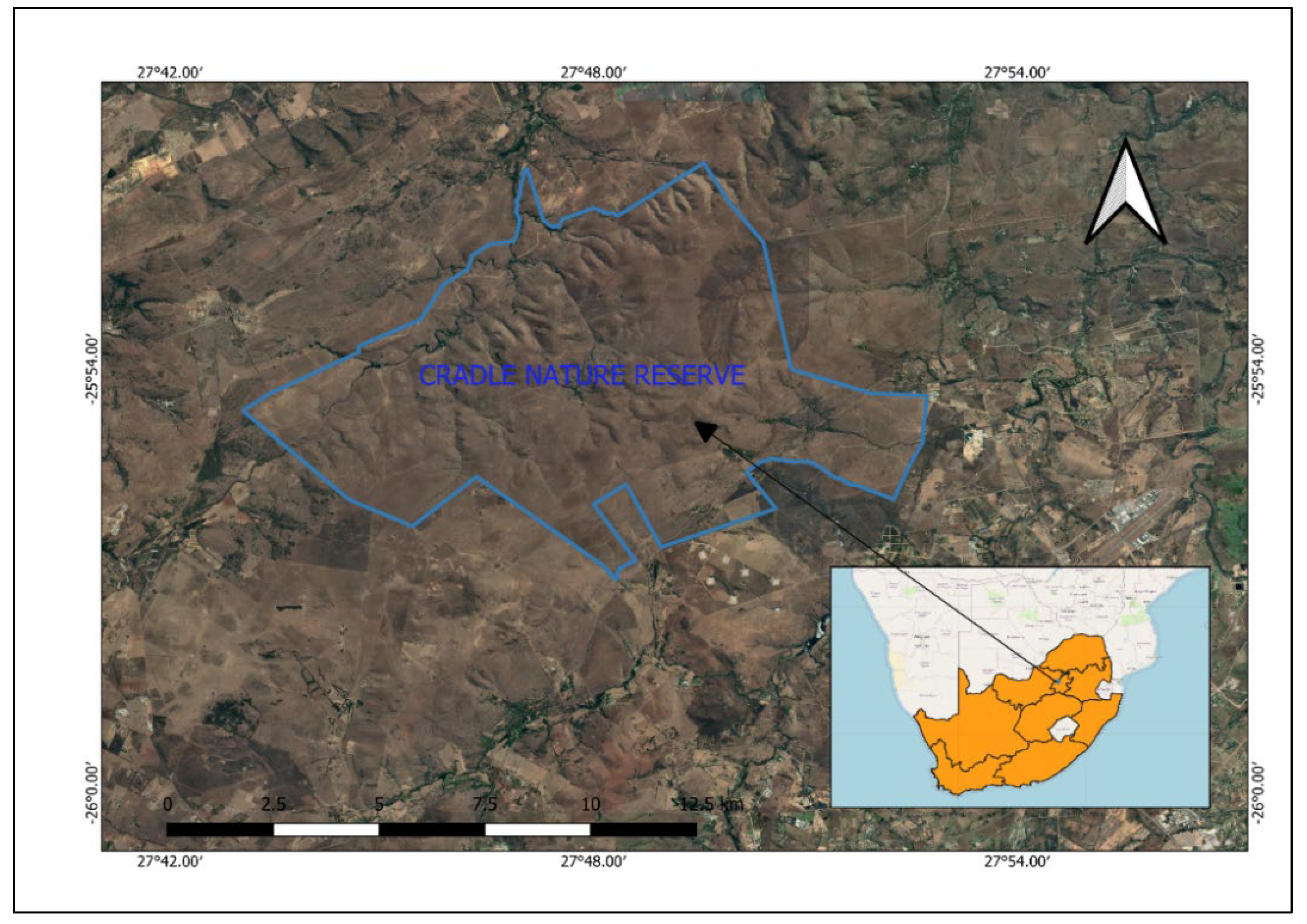
Figure 1. Study Area—Cradle Nature Reserve in South Africa with overview of the Google Earth Pro Imagery in UTM/WGS84 plane coordinate.
Remotesensing 15 05520 g001
Figure 2. Schematic of workflow for satellite data downloading, processing, XGBClassification, accuracy assessment, and QGIS processing.
Remotesensing 15 05520 g002
Figure 3. (a) XGBRFClassifcation image 1990; (b) XGBRFClassifcation mage 1998; (c) XGBRFClassifcation image 2009; (d) XGBRFClassifcation image 2015; (e) XGBRFClassifcation image 2020.
Remotesensing 15 05520 g003aRemotesensing 15 05520 g003bRemotesensing 15 05520 g003c
Figure 4. (a) LULC change 1990–1998; (b) LULC change area 1990–1998; (c) LULC change 1998–2009; (d) LULC change area 1998–2009; (e) LULC changes 2009–2015; (f) LULC change area 2009–2015; (g) LULC change 2015–2020; (h) LULC change area 2015–2020; (i) LULC change 1990–2020; (j) LULC change area 1990–2020.
Remotesensing 15 05520 g004aRemotesensing 15 05520 g004bRemotesensing 15 05520 g004cRemotesensing 15 05520 g004dRemotesensing 15 05520 g004eRemotesensing 15 05520 g004f
Table 2. Hyperparameters configurations.
HyperparameterValue
Number of decision trees20
Shrinkage (the shrinkage parameter controls the learning rate of the procedure)0.05
Sampling rate (the sampling rate for stochastic boosting)0.70
Maximum node (the maximum number of leaf nodes in each tree)20
Loss (loss function for regression)Least absolute deviation
Seed (the randomisation seed)0
Table 3. Hypotheses for landscape metrics.
Landscape Metric Hypothesis
Total Landscape Area (TA)The total landscape area for each class in the Cradle Nature Reserve has been altered by land cover degradation during the study period (1990 to 2020).
Landscape ProportionLand cover degradation has altered the proportion of landscape area for each class during the study period (1990 to 2020).
Patch DensityThere was an increase in landscape fragmentation in the study period (1990 to 2020) due to the rise in the number of patches per unit area.
Number of PatchesThere is an increase in landscape fragmentation in the study period (1990 to 2020) due to the rise in the total number of patches.
Largest Patch IndexOne class of land cover dominates during the period (1990 to 2020) in the study area.
Mean Patch AreaThere is a decrease in the average size of patches in each class due to land cover degradation during the study period (1990 to 2020).
Patch cohesion indexThere are no isolated classes (landscape class-connectivity) in the Cradle Nature Reserve landscape during the study period (1990 to 2020).
Shannon IndexThe Cradle Nature Reserve landscape is dominated by one land cover class during the study period (1990 to 2020).
Table 4. Accuracy assessment for Naïve Bayes and XGBRFClassifier for 2020 confusion matrix derivatives.
Naïve Bayes (lambda = 0.5)XGBRFClassifier
70%Producer’s AccuracyUser’s AccuracyF1Producer’s AccuracyUser’s AccuracyF1
Indigenous forest0.870.780.820.880.850.86
Open bush0.710.850.770.830.870.85
Natural grass0.910.820.860.920.930.92
Bare ground/rock outcrop0.820.860.840.950.920.93
Overall accuracy 0.83 0.90
Kappa index 0.76 0.86
30%
Indigenous forest0.880.780.830.780.780.78
Open bush0.70.810.750.720.770.74
Natural grass0.930.770.840.960.830.89
Bare ground/rock outcrop0.830.970.890.930.980.95
Overall accuracy 0.83 0.85
Kappa index 0.78 0.8
Table 5. Accuracy assessment for ground truthing confusion matrix derivatives.
Ground Truthing 2020
Producer’s AccuracyUser’s AccuracyF1
Indigenous forest0.930.930.93
Open bush0.770.900.83
Natural grass0.930.870.90
Bare ground/rock outcrop0.960.870.91
Overall accuracy 0.89
Kappa index 0.86
Table 6. Accuracy assessment for XGBRFClassifier confusion matrix derivatives.
XGBRFClassifier1990199820092015
70%Producer’s AccuracyUser’s AccuracyF1Producer’s AccuracyUser’s AccuracyF1Producer’s AccuracyUser’s AccuracyF1Producer’s AccuracyUser’s AccuracyF1
Indigenous forest0.930.970.950.910.890.900.860.960.910.920.900.91
Open bush0.950.920.930.840.910.870.900.840.870.820.890.85
Natural grass0.990.960.971.000.920.960.970.890.930.970.920.94
Bare ground/rock outcrop0.970.980.970.961.000.980.940.980.960.990.990.99
Overall accuracy 0.96 0.93 0.92 0.92
Kappa index 0.95 0.90 0.89 0.89
30%
Indigenous forest0.930.800.860.880.770.820.720.880.790.920.760.83
Open bush0.790.940.860.670.890.760.860.840.850.780.850.81
Natural grass0.920.920.921.000.810.900.970.840.900.900.900.90
Bare ground/rock outcrop1.000.950.970.941.000.970.910.910.910.901.000.95
Overall accuracy 0.91 0.87 0.88 0.87
Kappa index 0.88 0.82 0.84 0.83
Table 7. Land use–land cover spatial–temporal change detection matrices.
1990–1998 Land Cover Change Matrix (ha) 1998–2009 Land Cover Change Matrix (ha)
New ClassNew Class
Reference class1234Total1234Total
165.8571.830.320.08138.0860.7631.750.160.0092.67
225.77634.6478.940.00739.3545.08593.43532.510.081171.11
31.05464.406190.69396.547052.680.89216.776262.83135.256615.74
40.000.24345.80348.63694.671.2116.32467.39260.32745.24
Total92.671171.116615.74745.248624.77107.94858.287262.90395.658624.77
2009–2015 land cover change matrix (ha) 2015–2020 land cover change matrix (ha)
New classNew class
Reference class1234Total1234Total
192.9914.950.000.00107.9497.44129.840.970.00228.24
2129.43535.02184.948.89858.2811.88748.88328.192.991091.93
35.82538.826100.92617.357262.900.00217.665421.77727.396366.82
40.003.1580.96311.54395.650.002.42522.09413.26937.78
Total228.241091.936366.82937.788624.77109.311098.806273.011143.648624.77
1990–2020 land cover change matrix (ha)
New class Key
Reference class1234Total Class Value
171.9966.090.000.00138.08 Indigenous forest1
236.03598.76104.140.40739.35 Open bush 2
31.29427.005758.60865.797052.68 Natural grassland3
40.006.95410.27277.45694.67 Bare ground/rock outcrop4
Total 109.311098.806273.011143.648624.77
Table 8. Landscape metrics from 1990 to 2020.
Landscape Matrices May 2020
ClassTotal Landscape Area (ha)Landscape ProportionPatch DensityNumber of PatchesLargest Patch IndexMean Patch areaPatch Cohesion IndexMetricValue
Indigenous forest123.571.282.061980.070.628.03DIV_SH0.82Shannon Index
Open bush1229.2212.764.063912.483.149.59
Natural grassland6989.4072.551.6816269.2143.149.94
Bare ground/rock outcrop1292.1313.416.766513.131.989.63
Total 1402
Landscape Matrices May 2015
ClassTotal Landscape Area (ha)Landscape ProportionPatch densityNumber of PatchesLargest Patch IndexMean patch areaPatch cohesion indexMetricValue
Indigenous forest254.072.643.563430.150.748.52DIV_SH0.83Shannon Index
Open bush1236.1512.839.499142.481.359.52
Natural grassland7091.0173.602.4423570.3430.179.94
Bare ground/rock outcrop1053.0910.935.154961.022.129.43
Total 1988
Landscape Matrices May 2009
ClassTotal Landscape Area (ha)Landscape ProportionPatch densityNumber of PatchesLargest Patch IndexMean patch areaPatch cohesion indexMetricValue
Indigenous forest121.501.262.232150.070.577.91DIV_SH0.57Shannon Index
Open bush961.929.988.878551.011.139.23
Natural grassland8103.9684.121.1911583.4970.479.95
Bare ground/rock outcrop446.944.644.574400.261.028.87
Total 1625
Landscape Matrices May 1998
ClassTotal Landscape Area (ha) (ha)Landscape ProportionPatch densityNumber of PatchesLargest Patch IndexMean patch areaPatch cohesion indexMetricValue
Indigenous forest106.291.101.791720.060.627.80DIV_SH0.74Shannon Index
Open bush1309.0513.594.694525.222.909.73
Natural grassland7374.3376.541.6015475.3447.899.94
Bare ground/rock outcrop844.658.775.645430.661.569.16
Total 1321
Landscape Matrices May 1990
ClassTotal Landscape Area (ha)Landscape ProportionPatch densityNumber of PatchesLargest Patch IndexMean patch areaPatch cohesion indexMetricValue
Indigenous forest156.061.621.941870.120.838.40DIV_SH0.65Shannon Index
Open bush822.068.534.724550.781.819.34
Natural grassland7873.8381.731.0610281.0577.199.94
Bare ground/rock outcrop782.378.125.395190.811.519.34
Total 1263
Disclaimer/Publisher’s Note: The statements, opinions and data contained in all publications are solely those of the individual author(s) and contributor(s) and not of MDPI and/or the editor(s). MDPI and/or the editor(s) disclaim responsibility for any injury to people or property resulting from any ideas, methods, instructions or products referred to in the content.