Abstract
Recently, hyperspectral image classification has made great progress with the development of convolutional neural networks. However, due to the challenges of distribution shifts and data redundancies, the classification accuracy is low. Some existing domain adaptation methods try to mitigate the distribution shifts by training source samples and some labeled target samples. However, in practice, labeled target domain samples are difficult or even impossible to obtain. To solve the above challenges, we propose a novel dual-attention deep discriminative domain generalization framework (DAD3GM) for cross-scene hyperspectral image classification without training the labeled target samples. In DAD3GM, we mainly design two blocks: dual-attention feature learning (DAFL) and deep discriminative feature learning (DDFL). DAFL is designed to extract spatial features by multi-scale self-attention and extract spectral features by multi-head external attention. DDFL is further designed to extract deep discriminative features by contrastive regularization and class discrimination regularization. The combination of DAFL and DDFL can effectively reduce the computational time and improve the generalization performance of DAD3GM. The proposed model achieves 84.25%, 83.53%, and 80.63% overall accuracy on the public Houston, Pavia, and GID benchmarks, respectively. Compared with some classical and state-of-the-art methods, the proposed model achieves optimal results, which reveals its effectiveness and feasibility.
1. Introduction
With the continuous development of deep learning technology, remote sensing technology has made significant progress. Hyperspectral image (HSI) classification, as a branch of remote sensing, has been a major research topic for a long time. Now, it is widely used in environmental monitoring, the food industry, precision agriculture, land cover classification, and mineral exploration [1,2,3]. The purpose of HSI classification is to classify the pixels in HSIs into different categories based on their features. Conventional image classification models are not applicable for hyperspectral image classification. Despite the great success of these deep-learning-based works, some important challenges still exist.
On the one hand, the high data redundancies in hyperspectral images are caused by abundant bands and strong correlations among adjacent pixels. Therefore, effective feature extraction and representation learning are crucial to improve the classification accuracy. In the past, scholars have conducted research on remote sensing image segmentation, including traditional k-nearest neighbor [4], support vector machine [5,6], and convolutional neural network (CNN)-based algorithms [1]. Of these, the mainstream approaches are based on CNNs, which have outstanding feature extraction capabilities. However, models based on CNNs are data-driven and their training processes usually demand sufficient labeled samples with precise annotations. However, acquiring such a large amount of manually annotated samples will consume a tremendous amount of time and labor. Some works introduce the attention mechanism [7,8,9] to capture global and local features. However, the calculation times of these models are not taken into account. In practical applications, the calculation times of some tasks are strictly limited, such as defect detection in industrial products.
On the other hand, distribution shifts are another challenge that needs to be dealt with. As pointed out in [1,10,11], CNN-based methods are data-driven and trained in an entirely supervised manner. They extract features primarily by capturing the statistical relationships among the samples, where model generalization easily deteriorates for different distributions. As we know, data distributions between source and target domain samples are generally inconsistent because of differences in some factors (e.g., sensor nonlinearities, weather conditions, geographic locations, imaging conditions). As a consequence, the model performance suffers a catastrophic decrease. Domain adaptation is an effective and favored technique to remedy the above limitation, which tends to complete the target domain task by transferring knowledge learned from a label-scarce target domain and label-sufficient source domains. Recently, different domain adaptation methods have been proposed. They can be divided into three types from the perspective of whether the labeled target domain samples participate in training: supervised [12,13,14], semi-supervised [15,16], and unsupervised [17,18,19]. However, in practical applications, it is very difficult to obtain the labels of target domain samples. Thus, the above domain adaptation models may be unsuitable for some practical problems. Compared with domain adaptation, domain generalization (DG) is more practical but also more challenging, since it does not require the labeled target domain samples to participate in training. In 2023, the domain generalization method was first suggested for cross-scene hyperspectral image classification [10]. There are limited results on domain generalization for HSI classification, possibly due to the large and complex data, as well as the difficulty of annotating them and the fact that there are fewer standard datasets to use.
Considering that HSIs usually have large intra-class variance and high inter-class similarity and include heterogeneous spatial and spectral information, in this paper, we propose a novel dual-attention deep discriminative domain generalization model (DAD3GM) for hyperspectral image classification. In contrast to [10], we first design a dual-attention mechanism to extract important and multi-granularity features, instead of generating an extended domain as in [10]. Then, we enhance the model discriminability from the perspective of a feature extractor and a classifier, rather than only considering learning the discriminative features in the feature extractor. Specifically, we design a dual-attention feature learning (DAFL) module and a deep discriminative feature learning (DDFL) module. DAFL is designed to reduce the redundancies of HSIs and extract important domain-invariant spatial and spectral features, and it includes multi-scale self-attention to acquire coarse-grained and fine-grained spatial texture features and multi-head external attention to acquire robust spectral features with linear complexity. DDFL further enhances the learning of discriminative feature representations by contrastive regularization and class discrimination regularization. Our DAD3GM model has excellent generalization ability for hyperspectral image classification because it improves the model generalization by learning robust domain-invariant knowledge and enhancing the model discrimination. Our main contributions are summarized as follows.
- We propose a novel dual-attention deep discriminative domain generalization model for HSI classification, which considers the large intra-class variance, high interclass similarity, and heterogeneous spatial and spectral information present in HSIs.
- We develop a novel dual-attention module to effectively extract coarse-grained and fine-grained spatial texture features and important spectral features.
- We further design a deep discriminative feature learning module, incorporating feature discrimination learning and class discrimination learning. Firstly, to learn the discriminative features, contrastive regularization is implemented to separate the inter-class samples and compact intra-class samples as much as possible. Then, two independent classifiers are designed to further learn class discriminative features.
- Extensive experiments have been carried out on the three standard hyperspectral image classification datasets Houston, Pavia, and GID. Compared with the state-of-the-art methods, our model achieves optimal results.
2. Related Works
2.1. Domain Generalization
Domain generalization aims to reduce the distribution differences by transferring domain-invariant knowledge from source domains to an unseen target domain. Compared to domain adaptation (DA), it is more practical but also more challenging since the target images do not participate in training. The mainstream approaches generally can be divided into the following categories: domain-invariant representation learning [20,21,22], data augmentation [23,24,25], meta-learning [26,27,28], and ensemble learning [29,30,31]. For domain-invariant representation learning, adversarial learning [32] and minimize maximum mean discrepancy (MMD) [33] are the more popular strategies for the extraction of invariant information. Data augmentation is a common practice to improve algorithm generalization. Xu et al. [25] performed data augmentation by linearly mixing the amplitude information of different source domain samples to extract domain-agnostic knowledge and transferred them to target domain samples. Meta-learning tries to study episodes sampled from related tasks to benefit future learning. Chen et al. [26] took advantage of meta-knowledge to analyze the distribution shifts between source and target domains during testing. Most of these current investigations are mainly designed for nature images, which are not suitable for HSI work, since HSIs usually have the characteristics of large intra-class variance and high inter-class similarity and include heterogeneous spatial and spectral information.
2.2. Attention Mechanism
Attention mechanisms aim to imitate the human visual system that can capture the salient regions in complex scenes [34]. It can be treated as a dynamic weight adjustment process based on the features of inputs. Because of its outstanding merits, the attention mechanism has been widely applied to remote sensing tasks. Qin et al. [35] firstly adopted the discrete cosine transform from the perspective of the frequency domain to make up for the shortcomings of insufficient feature information caused by global average pooling in the most existing channel attention methods. Ding et al. [36] proposed a multi-scale receptive graph attention to extract the local–global adjacent node features and edge features. Zhao et al. [37] designed channel and spatial residual attention modules to integrate the multi-scale features by introducing a residual connection and attention mechanism. Paoletti et al. [38] employed channel attention to automatically design a network to extract spatial and spectral features. Shi et al. [39] proposed the 3D-OCONV method and abstracted the spectral features by combining 3D-OCONV and spectral attention. Pan et al. [40] applied an attention mechanism to extract global features and designed a multi-scale fusion module to extract local features, which effectively captured spatial features at different scales.
2.3. Contrastive Learning
Contrastive learning aims to extend the distance between the inter-class samples and reduce the distance between the intra-class samples, which can effectively improve the discriminative ability of networks. It has attracted widespread attention and has been employed for various tasks [41]. Recently, contrastive learning has also been introduced into the remote sensing field. Wang et al. [42] proposed the Contrastive-ACE network to capture the causal invariance through the causal affect from the features to labels and introduced the Contrastive-ACE loss to ensure cross-domain stable predictions. Ou et al. [43] proposed a HSI change detection framework, which built a loss on the foundation of self-supervised contrastive learning to extract better features. Guan et al. [3] developed a cross-domain contrastive learning framework to extract invariant features via the cross-domain discrimination task. Zhang et al. [44] implemented feature extraction by a 3D CNN and applied contrastive learning to learn more discriminative features so as to address the high inter-class similarity and large intra-class variance of HSIs. Jia et al. [45] designed a collaborative contrastive learning strategy to learn coordinated representations and achieve matching between LiDAR and HSI without labeled examples. This strategy adequately fused the LiDAR and hyperspectral data and effectively enhanced the classification accuracy of HSI and LiDAR data. Hang et al. [46] proposed a cross-modality contrastive learning algorithm for HSI classification, which extracted feature representations of hyperspectral and LiDAR images, respectively, and they designed a cross-modality contrastive loss to force features in the same patches to remain close.
3. Methods
Formally, a set of source domain examples is given as , where d represents the dimension of samples, denotes the number of samples, , and C denotes the total categories. The target domain is unlabeled. The purpose of the domain generalization-based HSI classification is to learn a domain-agnostic model G on the source domain samples, which can perform well on unlabeled target domain samples. The model contains a feature extractor and a classifier . In the following, we elaborate the proposed cross-scene HSI classification domain generalization method. The whole architecture is shown in Figure 1.
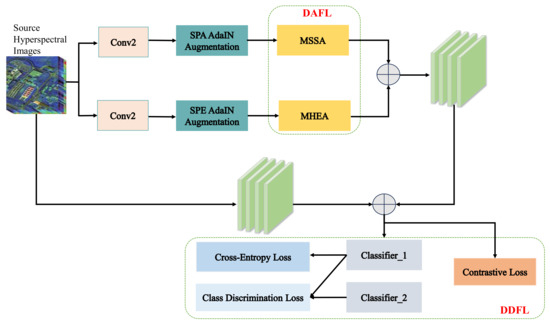
Figure 1.
The framework of the DAD3GM model. The model mainly contains two parts: DAFL and DDFL. DAFL contains MSSA and MHEA to extract import and robust domain-independent spatial and spectral features, respectively. DDFL contains a contrastive loss and class discrimination loss. DDFL is mainly used to excavate deep discriminative features.
3.1. Dual-Attention Feature Learning
Features play a critical role in enhancing model generalization. Domain-independent knowledge is robust and important in improving the true mapping between the inputs and its corresponding labels, while domain-related knowledge is unstable and may lead to false mapping between the inputs and labels. Hence, it is important to extract robust domain-independent spatial and spectral features. Data augmentation is a simple but effective technique that improves the model generalization ability by data transformation to generate more diverse samples. Among the data augmentation methods, adaptive instance normalization (AdaIn) [47] has a strong style transfer effect and is usually employed in conjunction with CNNs. Furthermore, morphological manipulations maintain the primary characteristics of the structure and shape information of an image by non-linearly transforming the features [1], in which dilation and erosion are the most basic and popular operations of morphological manipulation. Therefore, we firstly perform channel-wise AdaIn augmentation to generate diverse style spatial and spectral features, respectively, and then perform the morphological augmentation through the transformation of dilation and erosion to extract domain-independent structure feature representations. The AdaIn and morphological transformation can be expressed as in Equation (1) and Equation (2), respectively.
in which and represent the mean and standard deviation, respectively; denotes the spatial feature; denotes the adaptive learning parameter; and denotes the randomly selected spatial features. The augmented spectral images can be obtained in the same way:
in which and denote the structure elements of dilation and erosion, respectively; q and r denote the central pixel position of the current local patch.
After performing data augmentation, to effectively eliminate the data redundancies and the noise of the augmented source domain samples, a dual-attention feature learning (DAFL) module is designed to extract remarkable spatial and spectral features, respectively. DAFL incorporates multi-scale self-attention (MSSA) and spectral multi-head external attention (MHEA). Spatial components contain important texture and geometric features of a hyperspectral image and provide the most intuitive and basic information. For this reason, the MSSA module is devised to excavate the salient local and global spatial feature representations. The self-attention function can be computed on a query matrix Q, a key matrix K, and a value matrix V, where Q, K, V are acquired from the linear projection of the input X with parameter matrix , , . To obtain MSSA, different dilation rates in convolutions are set to obtain multi-scale and . Finally, MSSA can be calculated by Equation (3), and its structure is shown in Figure 2.
where D denotes the hidden dimension of the attention layer. The mutli-scale spatial attention feature maps can be expressed as in Equation (4):
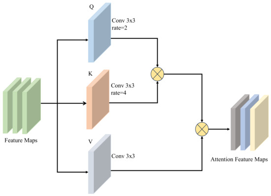
Figure 2.
The structure of multi-scale self-attention (MSSA). Q and K are set to different dilation rates to extract multi-scale attention feature maps.
The spectral images have abundant spectral bands, which possess rich information and can detect subtle changes and small differences in the spectra of objects. However, the spectral bands usually are redundant and will consume a lot of computing resources. To extract important and robust spectral feature representations as well as reduce the computing resources, the MHEA component is introduced, which is shown in Figure 3. MHEA can not only capture the correlations among all the samples, but also has linear complexity. Firstly, a single head external attention is implemented by two normalization layers, and two different training data memory units and are implemented by two linear layers without bias, which can be expressed as in Equation (5). not only can capture the latent relationships among all source domain samples, but also can provide powerful regularization and improve the generalization ability of the attention mechanisms. Secondly, is extended in a similar way as the multi-head attention in Transformer to obtain MHEA, which can be expressed as in Equation (6). With multiple sub-attention components, MHEA can learn the features with different weights, extract important spectral features more efficiently, and further reduce feature redundancies.
where represents the i-th head, H represents the number of heads, and denotes a linear transformation matrix making the dimensions of the input and output consistent. The augmented, important spatial and spectral features are fused by concoction. Then, to ensure the reliability, the augmented and original samples are fed into a two-layer convolution network for feature extraction by means of sharing weights.
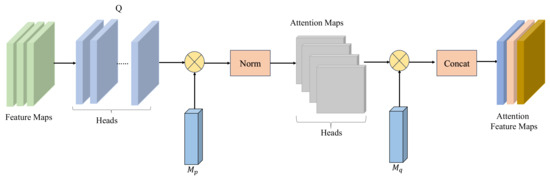
Figure 3.
The structure of multi-head external attention (MHEA).
3.2. Deep Discriminative Feature Learning
HSIs have complex characteristics such as high inter-class similarity and large intra-class variance, which may affect model discrimination and the classification accuracy. Nevertheless, discrimination plays a crucial role in model robustness. In view of this, we excavate the deep discriminative features from two aspects: discriminative feature representation learning and discriminative classifier representation learning. Firstly, supervised contrastive learning is implemented on the spatial and spectral features in order to obtain discriminative and robust domain-invariant knowledge:
where denotes each embedding feature in the batch size, and the features from the same class belong to positive samples and are denoted by ; denotes the number of positive sample sets, and the features outside the class pertain to negative samples and are denoted by ; and denote the positive and negative samples, respectively; and T is a scalar temperature parameter.
Secondly, inspired by the maximum classifier discrepancy (MCD) [48], two independent classifiers, and , are introduced to further enhance the classifier’s discrimination. Under such circumstances, a sample needs to be retrained if the predictions of the two classifiers are inconsistent. The difference loss function of the two classifiers can be expressed as
3.3. Training Process
In this paper, the classification loss adopts the standard cross-entropy loss function
where is the label of i-th sample , and c denotes the index of the class.
The total loss of DAD3GM consists of the classification loss , supervised contrastive loss , and classifier difference loss :
4. Experiments
In this section, our model is evaluated on standard cross-scene HSI benchmarks, namely the Houston, Pavia, and GID datasets. Moreover, some existing state-of-the-art methods are applied for comparison with ours, such as SDEnet [10], DANN [49], MRAN [50], DSAN [51], PDEN [52], HTCNN [53], SagNet [54], and LDSDG [55].
4.1. Datasets and Evaluation Metrics
(1) Houston Dataset: The Houston benchmark [56] comes from the University of Houston and the neighboring areas. It contains Houston13 and Houston18. The Houston13 dataset includes 144 spectral bands, and the pixels are . Its wavelength ranges from 380 to 1050 nm. The image spatial resolution is 2.5 m. Compared with Houston13, the spectral bands and image spatial resolution of Houston18 data are 48 and 1 m, respectively. To align them with Houston18, 48 spectral bands from Houston13 are selected, and the overlapping area is . Here, Houston13 and Houston18 are adopted as the source and target domains, respectively. The Houston benchmark has 7 categories, including residential buildings, grass healthy, trees, non-residential buildings, water, road, and grass stressed. The source domain comprises the Houston13 data, and the target domain comprises the Houston18 data. The total number of data of Houston13 and Houston18 is 2530 and 53,200, respectively. The details of the Houston data are shown in Table 1. The ground-truth images of the Houston benchmark are illustrated in Figure 4.

Table 1.
Classes and numbers of Houston data.
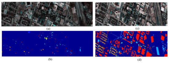
Figure 4.
The benchmark of Houston. (a,b) denote the image and ground truth of Houston13, respectively. (c,d) denote the image and ground truth of Houston18, respectively.
(2) Pavia Dataset: The Pavia benchmark [10] was captured by a reflective optics system imaging spectrometer sensor over Pavia, including the University of Pavia (UP) and Pavia Center (PC). One UP image includes pixels. Furthermore, it has a 1.3 m spatial resolution and 103 spectral bands. One PC image includes pixels and 102 bands. Note that, to ensure the same bands between the UP data and PC data, the 103rd band of the UP data was deleted. The Pavia benchmark contains 7 classes, including tree, bitumen, asphalt, meadow, brick, bare soil, and shadow. The UP data are employed as the source domain, and the PC data are employed as the target domain. The total numbers of UP and PC data are 39,332 and 39,355, respectively. The details of the Pavia data are shown in Table 2. The ground-truth images of the Pavia benchmark are shown in Figure 5.
Table 2.
Classes and numbers of Pavia data.
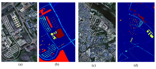
Figure 5.
The benchmark of Pavia. (a,b) denote the image and ground truth of the University of Pavia (UP), respectively. (c,d) denote the image and ground truth of the Pavia Center (PC), respectively.
(3) GID Dataset: The GID benchmark [57] was captured by the GF-2, which is the second satellite of the high-definition Earth observation system launched by the China National Space Administration. It was bulit by Wuhan University. It includes multi-spectral images taken at different times in many regions of China. The GID-nc dataset was collected on 3 January 2015 in Nanchang City, Jiangxi Province. GID-nc includes pixels. It contains four bands, including blue (0.45–0.52 m), green (0.52–0.59 m), red (0.63–0.69 m), and near-infrared (0.77–0.89 m). The spatial resolution of GID-nc is 4 m. GID-wh was taken on 11 April 2016 in Wuhan City, Hubei Province. GID-wh contains pixels. GID-wh has the same spectral and spatial resolution as GID-nc. Both of the two datasets have five categories: rural residential, irrigate land, garden land, river, and lake. The total numbers of GID-nc and GID-wh data are 23,339 and 30,812, respectively. We choose GID-nc as the source domain and GID-wh as the target domain. The details of the GID data are shown in Table 3. The ground-truth images of the GID benchmark are shown in Figure 6.
Table 3.
Classes and numbers of GID data.
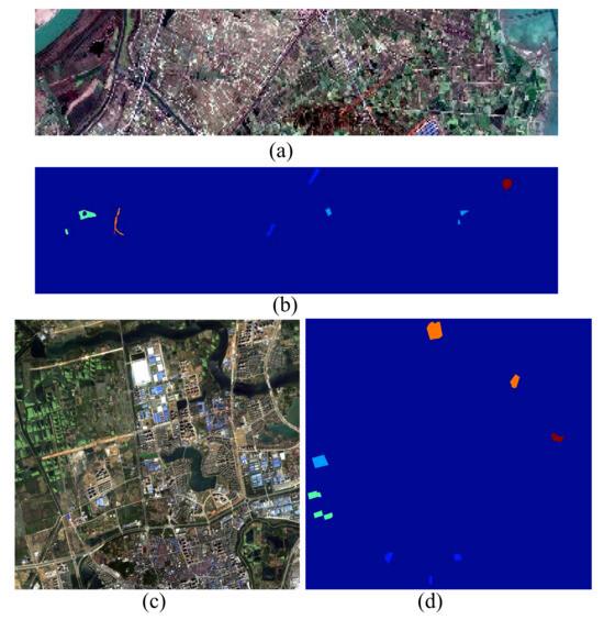
Figure 6.
The benchmark of GID. (a,b) denote the image and ground truth of GID-nc, respectively. (c,d) denote the image and ground truth of GID-wh, respectively.
(4) Evaluation Metrics: With regard to the evaluation metrics, the standard and public metrics kappa coefficient (KC) [58], overall accuracy (OA) [59], class-specific accuracy (CA) [10], and T-SNE [60] are employed to assess the model performance. KC denotes the proportion of error reduction between classification and completely random classification. In practice, the value range of KC is (0,1). OA is used to represent the classification accuracy. T-SNE is applied to visualize the high-dimensional data and intuitively reflect the distribution of features before and after DA and DG, and it can be used to analyze the performance of DA and DG. The mathematical representations of these metrics can be expressed as follows:
where represents the number of true labels of the k-th class, denotes the number of prediction labels of the k-th class, K denotes the total number of classes, and N represents the number of samples. TP represents the true positives, TN represents the true negatives, and FP represents the false positives.
4.2. Implementation Details
The experiments are implemented using the Pytorch [61] framework and are performed with an Nvidia 1080Ti GPU with 11 GB memory. The backbone is composed of two stacked Conv2d-ReLU-Maxpool2D components. The training parameter sets of the Houston, Pavia, and GID datasets are the same. The samples are divided into many patches with a size of . The network backbone comprises a series of Conv2d-ReLUMaxPool2d components, which is similar to the work in [10]. The learning rate is 0.001, the batch size is 256, and the max epoch is 400; the embedding feature dimension d_se is set to 64, both and are 1.0, and the convolution dilation rate in and is set to 2 and 4, respectively. The optimal strategy is adaptive moment estimation, with the momentum 0.9.
4.3. Comparison with the State-of-the-Art Methods
The results on the target domain Houston18 data are reported in Table 4. Compared with the existing methods, the proposed DAD3GM model achieves state-of-the-art results. It gains OA of 84.25% and yields 13.8% higher accuracy than DANN and 10.02% higher accuracy than LDSDG. It shows an improvement of 4.29% compared to the sub-optimal SDEnet. In terms of the KC performance, the proposed model is again optimal. It reaches 68.07%, yielding a 14.21% gain over DANN, which also is higher than the value of 60.18% for the HTCNN.
Table 4.
Performance comparisons for the target domain Houston18 data.
The results on the target scene Pavia Center data are reported in Table 5. Our model also has an obvious advantage compared with other methods. In terms of the OA performance, our model achieves increases of 1.59% and 12.65% compared to SDEnet and LDSDG, respectively. On the KC metric, our model shows increases of 1.96% and 20.53% compared to SDEnet and DANN, respectively. These results proves that our model is feasible and steady.
Table 5.
Performance comparisons for the target domain Pavia Center data.
The results on the target domain GID-wh data are reported in Table 6. Compared with the existing methods, the proposed DAD3GM model achieves state-of-the-art results. It gains OA of 80.63% and yields 11.82% higher accuracy than DANN and 4.52% higher accuracy than LDSDG, with an improvement of 2.68% over the sub-optimal SDEnet. In terms of the KC performance, the proposed model is again optimal. It reaches 75.73%, yielding a 17.69% gain over DANN and a 33.0% gain over HTCNN.
Table 6.
Performance comparisons on the target domain GID-wh data.
4.4. Ablation Experiments
(1) The Influence of Different Components: In this section, we analyze the influence of different parts on the target domain Pavia Center data. First of all, we start from the baseline without any strategies. To the baseline, the DAFL module is added to form Model A. On the basis of Model A, DDFL is added to form the proposed DAD3GM. The influence results on the target domain PaviaC data are reported in Table 7. In Table 7, - indicates that DAFL or DDFL is not introduced in the models, and ✓ indicates that DAFL or DDFL is introduced in the models. Regarding the metric OA, Model A shows an increase of 2.55% over the baseline. DAD3GM improves by 0.63% compared to Model A. Regarding the metric KC, Model A shows an increase of 3.09% over the baseline. DAD3GM improves by 0.82% compared to Model A. All of these modules contribute to improving the performance of our model, which fully demonstrates its high effectiveness and validity.
Table 7.
Performance comparisons for the target domain PC data.
(2) Parameter Analysis: In this part, we analyze the influence of some hyperparameters, including the embedding dimension d_se and the dilation rate and , . The influence of d_se is reported in Table 8. At first, with the increasing d_se, the OA and KC are constantly improving, whereas the OA and KC values decrease when d_se>64. Furthermore, the model not only achieves the best performance on the OA and KC, but also has outstanding performance on certain categories, such as 3, 4, 5, 6. Therefore, the d_se is set to 64 in our work.
Table 8.
Performance comparisons on the target domain Pavia data.
The influence of dilation rate is reported in Figure 7. When , both OA and KC achieve the optimal performance, increasing by 3.18% and 3.91%, respectively. Then, with the increase in , the OA and KC start to decrease. Compared with , when and , the OA reduces by 1.41% and 2.72%, respectively. Compared with , when and , KC reduces by 1.88% and 3.20%, respectively. We believe that the features extracted at a large scale may be poor because the size of each patch is . Thus, the is set to (2, 4).
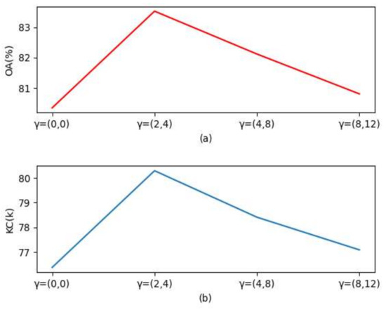
Figure 7.
The influence of different dilation rates . (a,b) denote the results of different in OA and KC, respectively.
The influence of and is reported in Figure 8. Firstly, we fix and analyze the influence of . When both and are equal to 1, the OA is 83.53% and the model achieves optimal performance. When is set to 0.3, 10, and 20, respectively, the OA drops between 2.58% and 3.32% compared with the best result of 83.53%. When is set to 0.1, 0.2, and 0.5, respectively, the OA drops between 0.2% and 1.94%. Then, we fix and analyze the influence of . In the beginning, the OA improves with the increasing . When and , the OA achieves the highest value. When the value of exceeds 1, the OA keeps decreasing with the increasing . When , the OA is the lowest and decreases by 2.98% compared with the best result of 83.53%. All of the results indicate that the discriminative features have a certain influence on the model’s generalization performance.
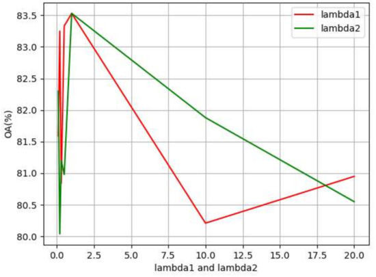
Figure 8.
The compared results of different values of and .
(3) Feature Visualization: To have a deeper and more intuitive understanding of the proposed method, we use T-SNE to visualize the features on the Houston data, which are shown in Figure 9. In addition, we compare our method with the existing SDENet model, which contains a source domain, extended domain, and target domain. The features from Figure 9a–f are extracted by the SDENet model, and the features in Figure 9g–h are extracted by our model, DAD3GM. From Figure 9a,c,e,g, we can see that the features of all categories are intertwined. From Figure 9b,d,f,h, we can see that the features of each class form their own clusters and they are separated from the features of the other categories. However, from Figure 9b, we can see that some features of classes 1, 2, and 3 are mixed together, and the features of classes 5 and 6 are mixed together. In addition, the features of class 6 form two clusters. From Figure 9d, we can see that the features of classes 1, 2, 3, 5, and 6 form two clusters, and some features of classes 1 and 3 are mixed together. From Figure 9f, we can see that some features of classes 1, 2, and 3 are mixed together; some features of classes 5, 6, and 7 are mixed together; and the features of class 6 form two clusters. Figure 9b,d,f reveal that the discriminability of the SDENet method is relatively poor, which may lead to the misclassification of some samples. From Figure 9h, we can see that the clusters formed by the features of each class are more compact and maintain a certain distance from the feature clusters of the other classes. These results reveal that our model has better discriminability.
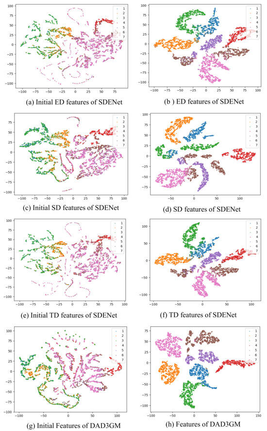
Figure 9.
T-SNE visualization of Houston data. (a,b) denote the ED features of SDENet, respectively. (c,d) denote the SD features of SDENet, respectively. (e,f) denote the TD features of SDENet, respectively. (g,h) denote the features of the proposed model DAD3GM, respectively.
(4) Computational Time: The computational times of one epoch of training in different models on the Houston18 and Pavia Center data are illustrated in Figure 10. For both the Houston18 and the Pavia Center data, the computational time of the PDEN model is the greatest. The computational time of the SagNet model is the smallest. Compared with SagNet, the computational time of our model increases by 3.13 s and 9.21 s on the Houston18 and Pavia Center data, respectively. However, comapred with SagNet, the OA of our model improves by 11.14% and 14.25% on the Houston18 and Pavia Center data, respectively. Compared with SDENet, the computional time of our model increases by 1.35 s and 0.88 s on the Houston18 and Pavia Center data, respectively. However, compared with SDENet, the OA of our model improves by 4.29% and 1.59% on the Houston18 and Pavia Center data, respectively. Compared with PDEN, the computational time of our model reduces by 76.78 s and 112.99 s on the Houston18 and Pavia Center data, respectively. Compared with the other methods, the computational time of our model is smaller, but the model performance is greatly improved.
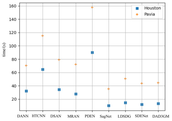
Figure 10.
The computational time of one epoch of training in the proposed model and compared with other methods on the Houston and Pavia data.
5. Discussion
Hyperspectral images have a lot of bands and the adjacent bands have strong correlations, which may lead to data redundancies, and it takes a deal deal of computing resources to process these redundant data. Furthermore, all the hyperspectral images are taken at different times and places. Affected by the weather or equipment, the data distributions are inconsistent, which leads to a sharp decline in model performance. In order to address these issues, we develop DAD3GM, which introduces a dual-attention mechanism to reduce the data redundancies and extract excellent global and local features, and we design a deep discriminative feature learning module based on contrastive learning to improve the discrimination of the proposed model. Experiments show that the combination of the dual-attention module and the deep discriminative feature learning module has advantages in hyperspectral image classification. In the previous hyperspectral image classification works, some researchers extracted features based on manual feature extraction, which is complex and consumes time; some works extracted features based on CNN networks, which improve the classification accuracy but suffer from the challenge of distribution shifts. Different from the previous works, we first select the important global and local augmented features by AdaIN through designing a dual-attention module including multi-scale self-attention and spectral multi-head external attention. From Table 7, we can see that the OA improves by 2.55% and the KC improves by 3.09% on the Houston data. Furthermore, we believe that the model discrimination also plays an important role in improving model generalization. Thus, we introduce a deep discriminative feature learning module by designing two classifiers. From Table 7, we can see that the OA improves by 0.63% and the KC improves by 0.82% after adding the discriminative module on the Houston data. We also visualize the feature distributions to show the feature distributions and compare our model with SDENet. From Figure 9, we can see that the features of each class form their own clusters and are separable from other classes, which reveals that our model has stronger discriminability. From Figure 10, we can see that the execution time of our model reduces by 76.78 s compared to PDEN, but the OA improves by 8.85%, which demonstrates that our model is more simple and effective. In conclusion, our work has investigated the issues of data redundancies and distribution shifts and the new modules has effectively improved the model’s generalization. The proposed framework is plug-and-play and can be extended to other tasks, such as object detection in hyperspectral images.
6. Conclusions
This paper proposes a simple but effective dual-attention deep discriminative domain generalization framework for hyperspectral image classification. The model adopts a dual-attention mechanism and deep discriminative feature representation learning module to learn discriminative domain invariant knowledge. The dual-attention module is designed with multi-scale self-attention and multi-head external attention to extract important spatial and spectral features, respectively. The dual-attention module is simple but effective and serves to reduce the data redundancies and model complexity. Then, a deep discriminative feature learning module is introduced to improve the generalization ability of the model by designing a contrastive regularization component and two independent classifiers. Compared with some existing state-of-the-art methods, our model achieves excellent performance. For example, compared with SDEnet, the overall accuracy and kappa coefficient of our method on the Pavia dataset are 85.53% and 80.29%, i.e., 1.59% and 1.96% higher than those of the SDEnet method, respectively, while taking a similar amount of time. Although the proposed method achieves state-of-the-art performance compared with the existing methods, it has some limitations, such as catastrophic forgetting and causal feature representation learning. In the future, we will perform knowledge distillation on the model parameters to resolve the catastrophic forgetting and introduce causal inference to build the causal relationships between the inputs and the labels, so as to further improve the model generalization on cross-domain hyperspectral images.
Author Contributions
Conceptualization, Q.Z., B.W. and S.L.; Methodology, X.W.; Experiments, X.W.; Data analysis, Q.Z., X.W. and S.L.; Writing—original draft preparation, X.W.; Writing—review and editing, Q.Z. and B.W; Supervision, L.W. and W.L. All authors have read and agreed to the published version of the manuscript.
Funding
This work was supported by the Pre-Research Project on Civil Aerospace Technologies of China National Space Administration (Grant No. D010301).
Data Availability Statement
Public available datasets were analyzed in the work and can be found at https://hyperspectral.ee.uh.edu/?page_id=459, accessed on 4 September 2023, https://www.ehu.eus/ccwintco/index.phptitle=Hyperspectral_Remote_Sensing_Scenes, accessed on 4 September 2023 and http://www.captain-whu.com/repository.html, accessed on 4 September 2023.
Conflicts of Interest
We state that we do not have known competing financial interests or personal relationships that may have influenced the work in this paper.
Abbreviations
The following abbreviations are used in this manuscript:
| DG | Domain Generalization |
| DA | Domain Adaptation |
| DAD3GM | Dual-Attention Deep Discriminative Domain Generalization Framework |
| DAFL | Dual-Attention Feature Learning |
| DDFL | Deep Discriminative Feature Learning |
| CNN | Convolutional Neural Network |
| MMD | Minimize Maximum Mean Discrepancy |
| AdaIn | Adaptive Instance Normalization |
| MHEA | Multi-Head External Attention |
| MSSA | Multi-Scale Self-Attention |
| MCD | Maximum Classifier Discrepancy |
| UP | University of Pavia |
| PC | Pavia Center |
| KC | Kappa Coefficient |
| OA | Overall Accuracy |
| CA | Class-Specific Accuracy |
| T-SNE | T-Distributed Stochastic Neighbor Embedding |
References
- Ahmad, M.; Shabbir, S.; Roy, S.K.; Hong, D.; Wu, X.; Yao, J.; Khan, A.M.; Mazzara, M.; Distefano, S.; Chanussot, J. Hyperspectral Image Classification—Traditional to Deep Models: A Survey for Future Prospects. IEEE J. Sel. Top. Appl. Earth Obs. Remote Sens. 2022, 15, 968–999. [Google Scholar] [CrossRef]
- Li, J.; Li, X.; Yan, Y. Unlocking the Potential of Data Augmentation in Contrastive Learning for Hyperspectral Image Classification. Remote Sens. 2023, 15, 3123. [Google Scholar] [CrossRef]
- Guan, P.; Lam, E.Y. Cross-Domain Contrastive Learning for Hyperspectral Image Classification. IEEE Trans. Geosci. Remote Sens. 2022, 60, 5528913. [Google Scholar] [CrossRef]
- Chao, X.; Li, Y. Semisupervised Few-Shot Remote Sensing Image Classification Based on KNN Distance Entropy. IEEE J. Sel. Top. Appl. Earth Obs. Remote Sens. 2022, 15, 8798–8805. [Google Scholar] [CrossRef]
- Chen, G.; Krzyzak, A.; Qian, S. Hyperspectral imagery classification with minimum noise fraction, 2D spatial filtering and SVM. Int. J. Wavelets Multiresolution Inf. Process. 2022, 20, 2250025. [Google Scholar] [CrossRef]
- Zhu, X.; Li, N.; Pan, Y. Optimization Performance Comparison of Three Different Group Intelligence Algorithms on a SVM for Hyperspectral Imagery Classification. Remote Sens. 2019, 11, 734. [Google Scholar] [CrossRef]
- Yu, C.; Wang, F.; Shao, Z.; Sun, T.; Wu, L.; Xu, Y. DSformer: A Double Sampling Transformer for Multivariate Time Series Long-term Prediction. In Proceedings of the 32nd ACM International Conference on Information and Knowledge Management, CIKM 2023, Birmingham, UK, 21–25 October 2023; pp. 3062–3072. [Google Scholar]
- Dong, Y.; Liu, Q.; Du, B.; Zhang, L. Weighted Feature Fusion of Convolutional Neural Network and Graph Attention Network for Hyperspectral Image Classification. IEEE Trans. Image Process. 2022, 31, 1559–1572. [Google Scholar] [CrossRef]
- Bai, J.; Wen, Z.; Xiao, Z.; Ye, F.; Zhu, Y.; Alazab, M.; Jiao, L. Hyperspectral Image Classification Based on Multibranch Attention Transformer Networks. IEEE Trans. Geosci. Remote Sens. 2022, 60, 5535317. [Google Scholar] [CrossRef]
- Zhang, Y.; Li, W.; Sun, W.; Tao, R.; Du, Q. Single-Source Domain Expansion Network for Cross-Scene Hyperspectral Image Classification. IEEE Trans. Image Process. 2023, 32, 1498–1512. [Google Scholar] [CrossRef]
- Zhai, X.; Liu, J.; Sun, S. A Two-Branch Network Based on Pixel-Pair and Spatial Patch Model for Hyperspectral Image Classification. In Proceedings of the International Conference on Communication Technology, ICCT, Nanjing, China, 11–14 November 2022; pp. 1622–1626. [Google Scholar]
- Peng, Y.; Liu, Y.; Tu, B.; Zhang, Y. Convolutional Transformer-Based Few-Shot Learning for Cross-Domain Hyperspectral Image Classification. IEEE J. Sel. Top. Appl. Earth Obs. Remote Sens. 2023, 16, 1335–1349. [Google Scholar] [CrossRef]
- Wang, W.; Liu, F.; Liu, J.; Xiao, L. Cross-Domain Few-Shot Hyperspectral Image Classification With Class-Wise Attention. IEEE Trans. Geosci. Remote Sens. 2023, 61, 5502418. [Google Scholar] [CrossRef]
- Xu, Z.; Wei, W.; Zhang, L.; Nie, J. Source-Free Domain Adaptation for Cross-Scene Hyperspectral Image Classification. In Proceedings of the IEEE International Geoscience and Remote Sensing Symposium, IGARSS, Kuala Lumpur, Malaysia, 17–22 July 2022; pp. 3576–3579. [Google Scholar]
- Chen, S.; Zhan, R.; Wang, W.; Zhang, J. Domain Adaptation for Semi-Supervised Ship Detection in SAR Images. IEEE Geosci. Remote Sens. Lett. 2022, 19, 4507405. [Google Scholar] [CrossRef]
- Lasloum, T.; Alhichri, H.; Bazi, Y.; Alajlan, N. SSDAN: Multi-Source Semi-Supervised Domain Adaptation Network for Remote Sensing Scene Classification. Remote Sens. 2021, 13, 3861. [Google Scholar] [CrossRef]
- Cheng, Y.; Chen, Y.; Kong, Y.; Wang, X. Soft Instance-Level Domain Adaptation with Virtual Classifier for Unsupervised Hyperspectral Image Classification. IEEE Trans. Geosci. Remote Sens. 2023, 61, 5509013. [Google Scholar] [CrossRef]
- Yu, C.; Liu, C.; Song, M.; Chang, C. Unsupervised Domain Adaptation with Content-Wise Alignment for Hyperspectral Imagery Classification. IEEE Geosci. Remote Sens. Lett. 2022, 19, 5511705. [Google Scholar] [CrossRef]
- Tang, X.; Li, C.; Peng, Y. Unsupervised Joint Adversarial Domain Adaptation for Cross-Scene Hyperspectral Image Classification. IEEE Trans. Geosci. Remote Sens. 2022, 60, 5536415. [Google Scholar] [CrossRef]
- Zhou, K.; Liu, Z.; Qiao, Y.; Xiang, T.; Loy, C.C. Domain Generalization: A Survey. IEEE Trans. Pattern Anal. Mach. Intell. 2023, 45, 4396–4415. [Google Scholar] [CrossRef]
- Wang, Z.; Loog, M.; van Gemert, J. Respecting Domain Relations: Hypothesis Invariance for Domain Generalization. In Proceedings of the 25th International Conference on Pattern Recognition, ICPR, Milan, Italy, 10–15 January 2020; pp. 9756–9763. [Google Scholar]
- Shao, R.; Lan, X.; Li, J.; Yuen, P.C. Multi-Adversarial Discriminative Deep Domain Generalization for Face Presentation Attack Detection. In Proceedings of the IEEE Conference on Computer Vision and Pattern Recognition, (CVPR), Long Beach, CA, USA, 15–20 June 2019; pp. 10023–10031. [Google Scholar]
- Wang, W.; Liu, P.; Zheng, H.; Ying, R.; Wen, F. Domain Generalization for Face Anti-Spoofing via Negative Data Augmentation. IEEE Trans. Inf. Forensics Secur. 2023, 18, 2333–2344. [Google Scholar] [CrossRef]
- Wang, M.; Yuan, J.; Qian, Q.; Wang, Z.; Li, H. Semantic Data Augmentation based Distance Metric Learning for Domain Generalization. In Proceedings of the 30th International Conference on Multimedia, (ACM), Lisbon, Portugal, 10–14 October 2022; pp. 3214–3223. [Google Scholar]
- Xu, Q.; Zhang, R.; Zhang, Y.; Wang, Y.; Tian, Q. A Fourier-Based Framework for Domain Generalization. In Proceedings of the IEEE Conference on Computer Vision and Pattern Recognition, (CVPR), Nashville, TN, USA, 20–25 June 2021; pp. 14383–14392. [Google Scholar]
- Chen, J.; Gao, Z.; Wu, X.; Luo, J. Meta-causal Learning for Single Domain Generalization. In Proceedings of the IEEE Conference on Computer Vision and Pattern Recognition (CVPR), Vancouver, BC, Canada, 17–24 June 2023. [Google Scholar]
- Chen, K.; Zhuang, D.; Chang, J.M. Discriminative adversarial domain generalization with meta-learning based cross-domain validation. Neurocomputing 2022, 467, 418–426. [Google Scholar] [CrossRef]
- Shu, Y.; Cao, Z.; Wang, C.; Wang, J.; Long, M. Open Domain Generalization with Domain-Augmented Meta-Learning. In Proceedings of the IEEE Conference on Computer Vision and Pattern Recognition, Nashville, TN, USA, 20–25 June 2021; pp. 9624–9633. [Google Scholar]
- Mesbah, Y.; Ibrahim, Y.Y.; Khan, A.M. Domain Generalization Using Ensemble Learning. In Intelligent Systems and Applications: Proceedings of the 2021 Intelligent Systems Conference (IntelliSys), Virtual, 2–3 September 2011; Springer: Cham, Switzreland, 2021; Volume 294, pp. 236–247. [Google Scholar]
- Lee, K.; Kim, S.; Kwak, S. Cross-domain Ensemble Distillation for Domain Generalization. In Proceedings of the Computer Vision European Conference (ECCV), Tel Aviv, Israel, 23–27 October 2022; Volume 13685, pp. 1–20. [Google Scholar]
- Arpit, D.; Wang, H.; Zhou, Y.; Xiong, C. Ensemble of Averages: Improving Model Selection and Boosting Performance in Domain Generalization. Adv. Neural Inf. Proc. Syst. 2022, 35, 8265–8277. [Google Scholar]
- Wang, X.; Tan, K.; Pan, C.; Ding, J.; Liu, Z.; Han, B. Active Deep Feature Extraction for Hyperspectral Image Classification Based on Adversarial Learning. IEEE Geosci. Remote Sens. Lett. 2022, 19, 6011505. [Google Scholar] [CrossRef]
- Gretton, A.; Borgwardt, K.M.; Rasch, M.J.; Schölkopf, B.; Smola, A.J. A Kernel Method for the Two-Sample-Problem. Adv. Neural Inf. Process. Syst. 2006, 35, 513–520. [Google Scholar]
- Guo, M.; Xu, T.; Liu, J.; Liu, Z.; Jiang, P.; Mu, T.; Zhang, S.; Martin, R.R.; Cheng, M.; Hu, S. Attention mechanisms in computer vision: A survey. Comput. Vis. Media 2022, 8, 331–368. [Google Scholar] [CrossRef]
- Qin, Z.; Zhang, P.; Wu, F.; Li, X. FcaNet: Frequency Channel Attention Networks. In Proceedings of the IEEE/CVF International Conference on Computer Vision (ICCV), Montreal, QC, Canada, 10–17 October 2021; pp. 763–772. [Google Scholar]
- Ding, Y.; Zhang, Z.; Zhao, X.; Hong, D.; Cai, W.; Yang, N.; Wang, B. Multi-scale receptive fields: Graph attention neural network for hyperspectral image classification. Expert Syst. Appl. 2023, 223, 119858. [Google Scholar] [CrossRef]
- Zhao, J.; Hu, L.; Huang, L.; Wang, C.; Liang, D. MSRA-G: Combination of multi-scale residual attention network and generative adversarial networks for hyperspectral image classification. Eng. Appl. Artif. Intell. 2023, 121, 106017. [Google Scholar] [CrossRef]
- Paoletti, M.E.; Moreno-Álvarez, S.; Xue, Y.; Haut, J.M.; Plaza, A. AAtt-CNN: Automatic Attention-Based Convolutional Neural Networks for Hyperspectral Image Classification. IEEE Trans. Geosci. Remote Sens. 2023, 61, 5511118. [Google Scholar] [CrossRef]
- Shi, C.; Sun, J.; Wang, T.; Wang, L. Hyperspectral Image Classification Based on a 3D Octave Convolution and 3D Multiscale Spatial Attention Network. Remote Sens. 2023, 15, 257. [Google Scholar] [CrossRef]
- Pan, H.; Zhao, X.; Ge, H.; Liu, M.; Shi, C. Hyperspectral Image Classification Based on Multiscale Hybrid Networks and Attention Mechanisms. Remote Sens. 2023, 15, 2720. [Google Scholar] [CrossRef]
- Albelwi, S. Survey on Self-Supervised Learning: Auxiliary Pretext Tasks and Contrastive Learning Methods in Imaging. Entropy 2022, 24, 551. [Google Scholar] [CrossRef]
- Wang, Y.; Liu, F.; Chen, Z.; Wu, Y.; Hao, J.; Chen, G.; Heng, P. Contrastive-ACE: Domain Generalization through Alignment of Causal Mechanisms. IEEE Trans. Image Process. 2023, 32, 235–250. [Google Scholar] [CrossRef]
- Ou, X.; Liu, L.; Tan, S.; Zhang, G.; Li, W.; Tu, B. A Hyperspectral Image Change Detection Framework With Self-Supervised Contrastive Learning Pretrained Model. IEEE J. Sel. Top. Appl. Earth Obs. Remote Sens. 2022, 15, 7724–7740. [Google Scholar] [CrossRef]
- Zhang, S.; Chen, Z.; Wang, D.; Wang, Z.J. Cross-Domain Few-Shot Contrastive Learning for Hyperspectral Images Classification. IEEE Trans. Geosci. Remote Sens. 2022, 19, 5514505. [Google Scholar] [CrossRef]
- Jia, S.; Zhou, X.; Jiang, S.; He, R. Collaborative Contrastive Learning for Hyperspectral and LiDAR Classification. IEEE Trans. Geosci. Remote Sens. 2023, 61, 5507714. [Google Scholar] [CrossRef]
- Hang, R.; Qian, X.; Liu, Q. Cross-Modality Contrastive Learning for Hyperspectral Image Classification. IEEE Trans. Geosci. Remote Sens. 2022, 60, 5532812. [Google Scholar] [CrossRef]
- Oh, Y.; Ye, J.C. CXR Segmentation by AdaIN-Based Domain Adaptation and Knowledge Distillation. In Proceedings of the Computer Vision European Conference, (ECCV), Tel Aviv, Israel, 23–27 October 2022; Springer: Cham, Switzerland, 2022; Volume 13681, pp. 627–643. [Google Scholar]
- Saito, K.; Watanabe, K.; Ushiku, Y.; Harada, T. Maximum Classifier Discrepancy for Unsupervised Domain Adaptation. In Proceedings of the IEEE Conference on Computer Vision and Pattern Recognition, CVPR, Salt Lake City, UT, USA, 18–23 June 2018; pp. 3723–3732. [Google Scholar]
- Yu, C.; Wang, J.; Chen, Y.; Huang, M. Transfer Learning with Dynamic Adversarial Adaptation Network. In Proceedings of the IEEE International Conference on Data Mining, ICDM, Beijing, China, 8–11 November 2019; pp. 778–786. [Google Scholar]
- Zhu, Y.; Zhuang, F.; Wang, J.; Chen, J.; Shi, Z.; Wu, W.; He, Q. Multi-representation adaptation network for cross-domain image classification. Neural Netw. 2019, 119, 214–221. [Google Scholar] [CrossRef]
- Zhu, Y.; Zhuang, F.; Wang, J.; Ke, G.; Chen, J.; Bian, J.; Xiong, H.; He, Q. Deep Subdomain Adaptation Network for Image Classification. IEEE Trans. Neural Netw. Learn. Syst. 2021, 32, 1713–1722. [Google Scholar] [CrossRef] [PubMed]
- Li, L.; Gao, K.; Cao, J.; Huang, Z.; Weng, Y.; Mi, X.; Yu, Z.; Li, X.; Xia, B. Progressive Domain Expansion Network for Single Domain Generalization. In Proceedings of the IEEE Conference on Computer Vision and Pattern Recognition, CVPR, Nashville, TN, USA, 20–25 June 2021; pp. 224–233. [Google Scholar]
- He, X.; Chen, Y.; Ghamisi, P. Heterogeneous Transfer Learning for Hyperspectral Image Classification Based on Convolutional Neural Network. IEEE Trans. Geosci. Remote Sens. 2020, 58, 3246–3263. [Google Scholar] [CrossRef]
- Nam, H.; Lee, H.; Park, J.; Yoon, W.; Yoo, D. Reducing Domain Gap by Reducing Style Bias. In Proceedings of the IEEE Conference on Computer Vision and Pattern Recognition, CVPR, Nashville, TN, USA, 20–25 June 2021; pp. 8690–8699. [Google Scholar]
- Wang, Z.; Luo, Y.; Qiu, R.; Huang, Z.; Baktashmotlagh, M. Learning to Diversify for Single Domain Generalization. In Proceedings of the IEEE/CVF International Conference on Computer Vision, ICCV, Montreal, QC, Canada, 10–17 October 2021; pp. 814–823. [Google Scholar]
- Yokoya, N.; Ghamisi, P.; Xia, J.; Sukhanov, S.; Heremans, R.; Tankoyeu, I.; Bechtel, B.; Saux, B.L.; Moser, G.; Tuia, D. Open Data for Global Multimodal Land Use Classification: Outcome of the 2017 IEEE GRSS Data Fusion Contest. IEEE J. Sel. Top. Appl. Earth Obs. Remote Sens. 2018, 11, 1363–1377. [Google Scholar] [CrossRef]
- Tong, X.Y.; Xia, G.S.; Lu, Q.; Shen, H.; Li, S.; You, S.; Zhang, L. Land-Cover Classification with High-Resolution Remote Sensing Images Using Transferable Deep Models. Remote Sens. Environ. 2020, 237, 111322. [Google Scholar] [CrossRef]
- Warrens, M.J. Kappa coefficients for dichotomous-nominal classifications. Adv. Data Anal. Classif. 2021, 15, 193–208. [Google Scholar] [CrossRef]
- Fan, X.; Lu, Y.; Liu, Y.; Li, T.; Xun, S.; Zhao, X. Validation of Multiple Soil Moisture Products over an Intensive Agricultural Region: Overall Accuracy and Diverse Responses to Precipitation and Irrigation Events. Remote Sens. 2022, 14, 3339. [Google Scholar] [CrossRef]
- Rauber, P.E.; Falcão, A.X.; Telea, A.C. Visualizing Time-Dependent Data Using Dynamic t-SNE. In Proceedings of the 18th Eurographics Conference on Visualization, EuroVis 2016—Short Papers, Groningen, The Netherlands, 6–10 June 2016; pp. 73–77. [Google Scholar]
- Paszke, A.; Gross, S.; Chintala, S.; Chanan, G.; Yang, E.; Devito, Z.; Lin, Z.; Desmaison, A.; Antiga, L.; Lerer, A. Automatic differentiation in PyTorch. In Proceedings of the 31st Conference on Neural Information Processing Systems (NIPS 2017), Long Beach, CA, USA, 4–9 December 2017. [Google Scholar]
Disclaimer/Publisher’s Note: The statements, opinions and data contained in all publications are solely those of the individual author(s) and contributor(s) and not of MDPI and/or the editor(s). MDPI and/or the editor(s) disclaim responsibility for any injury to people or property resulting from any ideas, methods, instructions or products referred to in the content. |
© 2023 by the authors. Licensee MDPI, Basel, Switzerland. This article is an open access article distributed under the terms and conditions of the Creative Commons Attribution (CC BY) license (https://creativecommons.org/licenses/by/4.0/).