Abstract
Airborne LiDAR (Light Detection and Ranging) is an active Earth observing system, which can directly acquire high-accuracy and dense building roof data. Thus, airborne LiDAR has become one of the mainstream source data for building detection and reconstruction. The emphasis for building reconstruction focuses on the accurate extraction of feature lines. Building roof feature lines generally include the internal and external feature lines. Efficient extraction of these feature lines can provide reliable and accurate information for constructing three-dimensional building models. Most related algorithms adopt intersecting the extracted planes fitted by the corresponding points. However, in these methods, the accuracy of feature lines mostly depends on the results of plane extraction. With the development of airborne LiDAR hardware, the point density is enough for accurate extraction of roof feature lines. Thus, after acquiring the results of building detection, this paper proposed a feature lines extraction strategy based on the geometric characteristics of the original airborne LiDAR data, tracking roof outlines, normal ridge lines, oblique ridge lines and valley lines successively. The final refined feature lines can be obtained by normalization. The experimental results showed that our methods can achieve several promising and reliable results with an accuracy of 0.291 m in the X direction, 0.295 m in the Y direction and 0.091 m in the H direction for outlines extraction. Further, the internal feature lines can be extracted with reliable visual effects using our method.
1. Introduction
Buildings are essential components in urban areas. In recent years, the rapid development of city construction has led to an increasing number or frequent changes in buildings. The collection and update of information on these changes require a great deal of manpower, material and finance [1,2,3,4]. In order to improve this situation, how to promote the level of automatic building reconstruction has been a research hotspot, where building detection and roof feature lines extraction are the two important prerequisites and steps [5,6,7,8,9,10,11,12,13]. Airborne LiDAR (Light Detection and Ranging) is an active Earth observing system that is composed of an Inertial Measurement Unit (IMU), Global Positioning System (GPS), and a laser scanner [14]. It can acquire high-accuracy three-dimensional (3D) geospatial data of the Earth’s surface directly, especially dense roof data. Thus, airborne LiDAR data show great potential in building model reconstruction applications and have become one of the important data sources for building detection and reconstruction. Although most hardware and components integration problems in the airborne LiDAR field have been solved, algorithms and software for data postprocessing are still urgently needed in general. In recent decades, building-related studies have always been a research focus in LiDAR data processing, such as building detection, roof outlines extraction and building model reconstruction [6,8,15,16,17,18]. These research achievements are also very helpful for city planning, traffic planning, disaster evaluation, digital map updating and other applications. Compared with building detection and building model reconstruction, roof feature lines extraction seems to attract relatively less attention. Possible reasons may include the following:
(1) Early LiDAR data density is insufficient to determine the line structure inside the roof.
(2) As the intermediate step between building detection and reconstruction, there are two ways to accomplish roof feature lines extraction: (1) direct extraction from the original points and (2) intersection of the extracted planes. The latter one is the main way at present, which means the core element in this method is accurate extraction of the planes fitted by the corresponding points [17]. Once the two planes are determined, the corresponding intersection line can be uniquely determined too.
However, with the development of LiDAR hardware, the acquired data density is enough to extract feature lines directly. In addition, compared with the direct extraction method, intersection of the extracted planes is easier to bring in more errors from plane fitting. In particular for complex roofs, the appurtenances on the roof may affect the accuracy of plane fitting, such as dormer and solar water heater. Thus, in order to improve the accuracy, roof feature lines extraction is still a necessary and important step in LiDAR data postprocessing. If feature lines can be extracted precisely, the subsequent work, such as building modeling and reconstruction, will be conducted more accurately and smoothly. This paper focuses on roof feature lines extraction, and proposes a coarse-to-fine strategy based on the point cloud geometry. Unlike most previous feature lines extraction methods, our method can effectively extract outlines and inner lines of roofs from airborne LiDAR data directly, which is beneficial to the subsequent three-dimensional building’s modeling. The remaining contents of this paper are organized as follows: Section 2 briefly reviews the related work; Section 3 describes the principles and implementation steps of our proposed method in detail; Section 4 presents and analyzes the experimental results, as well as precision evaluation; and the main conclusions are provided in Section 5.
2. Related Work
Building roof feature lines are of two types in general: external and inner feature lines. The external feature lines are always termed as roof outline/boundary/contour. And the inner feature lines can be separated into two groups: ridge lines and valley lines, where the ridge lines can further be divided into normal ridge lines and oblique ridge lines, according to the spatial position of lines, as shown in Figure 1.
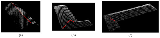
Figure 1.
The diagram of the internal roof feature lines, including (a) normal ridge lines, (b) oblique ridge lines and (c) valley lines.
The effective extraction of roof feature lines can provide a reliable and accurate three-dimensional model of buildings. As mentioned above, intersection of the extracted planes is the main method of extraction of the inner feature lines [2,15,17,19]. The current related literature of building feature lines extraction mainly focus on the external feature lines (or roof outlines) generally [5,18,20,21,22,23,24]. The reasons may include the following two aspects. On the one hand, the accurate roof outlines can be directly used to construct the simplified building model. For many application scenarios with low accuracy requirements, such as civil 3D map display, it is enough to meet the daily needs. On the other hand, compared with roof outlines, the precise extraction of the inner feature lines needs data support with much higher density. In addition, due to various roof types in reality, the extraction of the inner feature lines is more difficult than that of roof outlines.
Roof outlines extraction mainly includes three types of algorithms:
(1) Raster image processing methods
Compared with point cloud processing, there are various mature algorithms and operators of edge detection in the field of digital image processing. In order to apply these methods to airborne LiDAR data, the original point cloud data should be rasterized. Li [25] presented an automatic edge extraction method by LiDAR-optical fusion adaptive for complex building shapes. After detecting the points of each roof patch, the initial edges were extracted from images using the improved Canny detector [25], which was conducted by the edge location information from LIDAR point cloud in the form of edge buffer areas. Then, the roof patch and initial edges were integrated to form the ultimate complete edge by mathematical morphology. Cheng [26] presented an approach integrating high-resolution imagery and Lidar data for obtaining building boundaries with precise geometric position and details. A building image was generated by processing an original image using a bounding rectangle and a buffer, which were derived from the segmented LiDAR building points. Sun [27] combined the robust classification convolutional neural networks (CNN) and active contour model (ACM) to extract building boundary. Akbulut [28] combined LiDAR point cloud and aerial imagery and used initial contour positions to segment an object in the image. Initial contour positions were then detected by a series of image enhancements, band ratio and morphological operations. In general, rasterization from the original point clouds to images should be conducted first in these methods, which results in the loss of precision.
(2) Methods based on geometric properties of point cloud
The extraction of roof outlines is generally conducted on one single building. Algorithms of this type can obtain roof outlines by fitting several edge points extracted from the original LiDAR points [18,29]. In general, point clouds are organized by Triangulated Irregular Network (TIN) firstly [23]. Then, the outer points are grouped into edge points according to triangulation forms. Final roof outlines can be acquired after linear fitting and regularization. Zhang [30] adopted a tracing algorithm based on edge length ratio to refine the rough roof outlines fitted by the extracted edge points. Final outlines with higher precision were obtained further using regression analysis. Jaya [23] used a multiscale local geometric descriptor (LGD), computed using tensor voting and gradient energy tensor to enhance specific line-type features. The proposed three-step method is TIN generation, tensorline extraction, and postprocessing of the tensorlines to extract line segments in the roof. These methods are directly based on the original LiDAR data without rasterization, but they need much computation cost for constructing TIN. Further, concave outlines may not be preserved well using TIN-based methods. Li [15] proposed a Paired Point Attention (PPA) module to predict the true model edges from an exhaustive set of candidate edges between the vertices. However, due to the lack of building reconstruction data, they constructed a large-scale synthetic dataset to verify the effectiveness and robustness of the proposed method. In these methods, the high computation cost for constructing TIN cannot be ignored.
(3) Alpha-shape-based methods
Originally proposed by Edelsbrunner [31], the alpha-shape algorithm has been applied to outlines extraction of irregular point clouds widely nowadays. It is simple, highly efficient, stable and has high precision, suitable for most types of building outlines. The algorithm considers a parameter α that enables identification of pairs of points that compose edge segments. Each edge is then considered to compose the object boundary. An optimal α depends mainly on point density variation and the desired level of detail of the extracted boundary, as described in [7]. dos Santos [24] extracts building boundaries using the alpha-shape algorithm by applying five different strategies to determine the parameter α. The main advantage lies in its robustness to abrupt density variation, especially in regions with vegetation occlusion and overlapping strips. In alpha-shape-based methods, the essential step is to determine the parameter α value (that is the circle radius) [32]. Too big an α value may result in lower precision of the extracted outlines and the omission of some details, while too small an α value may fail to acquire enough edge points. Hence, the optimal α value is very essential in these methods.
3. Materials and Methods
As stated above, building roof lines are mainly of two types, external and internal feature lines. The corresponding extraction algorithms are described as follows in detail.
3.1. Datasets Description
The test dataset has six test areas. Areas 1 to 3, provided by ISPRS (International Society for Photogrammetry and Remote Sensing), are located in Vaihingen, Germany, with a density of 4 points/m2. As shown in Figure 2, the point data are colored by the height value of each point. The higher the point, the redder the color. The detailed introduction of this dataset can be found in [33]. In order to enrich roof types, Areas 4 to 6 are added herein. The three datasets are located in Alashan, China with a density of 5 points/m2. However, the corresponding orthophoto is absent. All of the experiments were implemented in Matlab 2014b and the results were displayed in LiDAR_suite v1.4 (software developed by the authors).
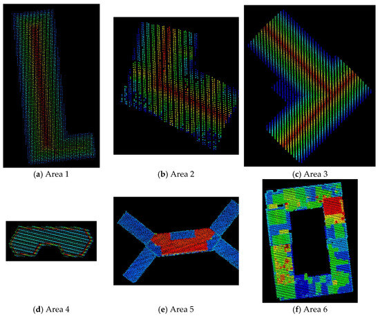
Figure 2.
Test data for extraction of building roof feature lines.
3.2. Extraction of External Feature Lines
Roof outlines extraction is a coarse-to-fine process. After detecting edge points and separating these points into several groups, the coarse roof outlines can be fitted sequentially. According to some established rules and experiences, the refined roof outlines can be acquired.
3.2.1. Coarse Roof Outlines
The steps of extracting the coarse roof outlines are listed as follows.
(1) Creating a grid index for the point cloud. The original three-dimensional point clouds should be firstly projected to two-dimensional XOY plane. The length and width of the grid depend on the max and min values of X and Y directions correspondingly. Grid cells are created at an interval of twice the average point spacing, which ensures an optimal extraction of edge points.
(2) Eliminating pseudo empty cells. In general, pseudo empty cells are corresponding to the void holes located inside the original roof due to loss of data, as red cells shown in Figure 3. These cells have an impact on the accurate extraction of edge points. Thus, these pseudo empty cells should be eliminated by counting the number of contiguous empty cells. For real roof edges, the empty cells should be the grey cells shown in Figure 3 with a relatively large quantity. As a result, if the number is too small (like 2 in Figure 3), these corresponding cells (red cells in Figure 3) can be considered as the pseudo empty cells and labeled to distinguish from the other cells.
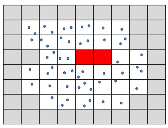
Figure 3.
The diagram of pseudo empty cells, where blue points represent the original point cloud, red cells represent the pseudo empty cells and grey cells represent the empty cells.
(3) Detecting edge points. Each grid should be judged. If there are empty grids in the eight neighbor grids of the current grid, then the points in this current grid can be detected as edge points.
(4) Detecting corner points. Corner points are used to separate edge points into several groups. This paper proposed a corner-point-detecting strategy based on the two-dimensional Euclidean distance, as shown in Figure 4.
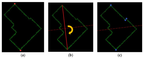
Figure 4.
The diagram of a corner-point-detecting strategy based on the two-dimensional Euclidean distance with three steps: (a) searching for the two farthest points, (b) forming a line segment connecting the two farthest points and rotating the line segment to generate several segments every 15 degrees rotation and (c) detecting the corner points.
The detail steps are listed as follows.
a. The two farthest points, and , in the edge point set are firstly detected as corner points, as shown in the red circles in Figure 4a. Adding them into the corner point set .
b. The line segment connecting and is labeled as , as shown in the red line in Figure 4b. The midpoint of is considered as the rotational center, and several segments are generated every 15 degrees rotation (an empirical value, in order to avoid omitting corner points), as shown in the red dotted line (corresponding to 90 degrees) in Figure 4b. Add these line segments into the lines set . Take as the beginning point, search all edge points clockwise and calculate the distances between each edge point and every line segment in . If the distance from the current edge point p to one certain line l is the maximum or minimum in the neighbor points of its circle neighborhood (the radius is set as twice or triple average point spacing according to the experience), p is considered as a candidate corner point, as shown in the blue circles in Figure 4c. If there is no p in , then add p into . It is noteworthy that if the distance between p and l is smaller than the average point spacing, p would not be considered as a candidate corner point.
c. Eliminate pseudo corner points. Search clockwise, and take three adjacent points into one group. As illustrated in Figure 5, if the angle of the current point (the red one) p is close to 180 degrees (±10 degrees, an empirical value), p should be considered as a pseudo corner point and eliminated from .
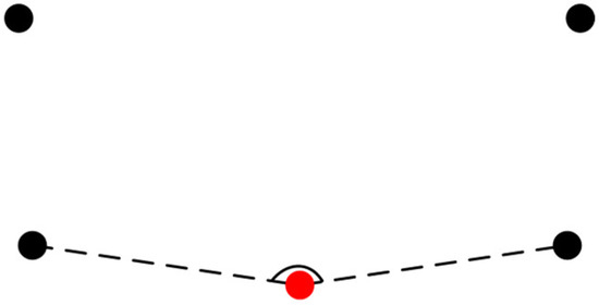
Figure 5.
Pseudo corner points elimination.
(5) Group fitting. Due to sequential storage, all edge points can be separated into several groups by the detected corner points, as shown in the yellow lines in Figure 6. In order to achieve stable line parameters, a gradient descent method is adapted to linear fitting.
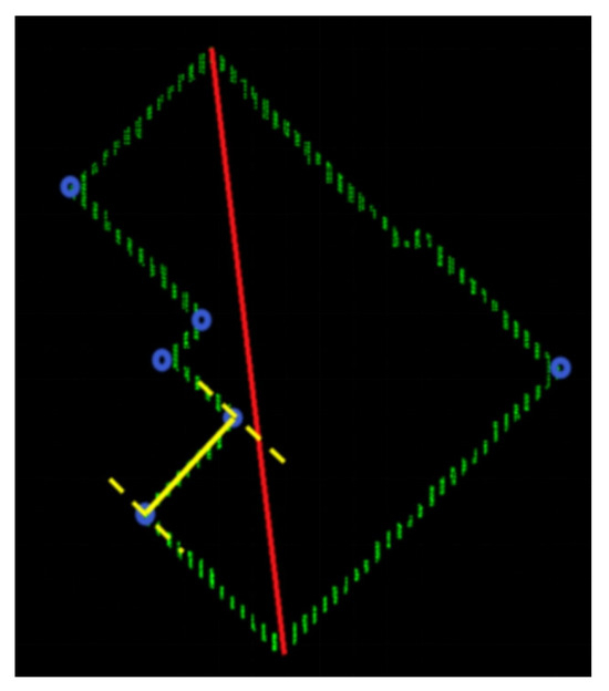
Figure 6.
Group fitting by the detected corner points.
(6) Finally, the initial XY coordinates of the intersection points can be acquired by intersecting the two adjacent roof outlines.
3.2.2. Refined Roof Outlines
In general, the two adjacent outlines of regular roofs are orthogonal to each other on the two-dimensional XOY plane, as the following equation shows, where k and k′ are the slope of the two adjacent outlines.
According to the principle, this paper adapted averaging strategy by separating those outlines into several groups. As the original LiDAR points cannot always fall to the real building outlines, real roofs are generally bigger than the area acquired by airborne LiDAR. Then, the extracted coarse outlines should be expanded after normalization to obtain more accurate outlines’ position. The details are listed as follows.
(1) Select one outline , which can be expressed as . Add into the slope set and label this outline. Given that the coordinates of the two endpoints are and , the slope of this outline can be calculated by the Formula (2):
(2) Take as the beginning outline, and search all outlines clockwise. According to the law of cosines, the included angle between and other unlabeled outlines can be acquired using the Formula (3), where and are the slope of the two outlines.
(3) If satisfies any of the following conditions ( in this paper),
- ①
- ②
- ③
Then these two outlines are considered parallel or orthogonal. Label the unlabeled outline and add its slope to . It is noteworthy that for the convenience of averaging the slope values, if the two outlines are orthogonal, its slope should be transformed using Formula (1) and stored.
(4) Calculate the average slope value and assign it to all values in . Similarly, for those orthogonal outlines, their slope values should be updated by the transformed value. Keep the coordinates of the center point of each line unchanged, new expression of each line can be acquired and stored.
(5) If there are still unlabeled outlines, repeat steps from (1) to (4); otherwise, proceed to step (6).
(6) For each outline , add neighbor points with double average point spacing of every edge point on into a temporary set , and then calculate value for all points in using the following formula.
Count the number of edge points or , respectively. The edge points in the group with less number are considered to be located outside the corresponding outline . Parallel move through the farthest outer edge point and obtain the expanded outline . Repeat this step for other outlines.
(7) Determine the final XYZ coordinates of corner points. The XY plane coordinates of each corner point are obtained by intersecting the adjacent outlines, and their height Z values are calculated by five nearest (the planar distance) original points using the inverse distance weighted (IDW) average algorithm. In general, the height change in edge points in their corresponding neighborhood should be continuous. However, there may be several appurtenances on the roof, such as dormer and lobby, which results in an abrupt height change in one certain point’s neighborhood, as shown in Figure 7; a height histogram will be adapted to separate the height values of its neighbor points into several groups (the interval can be set according to the point density, 0.1 m herein). Then, two or more corner points in the same planar position can be acquired.
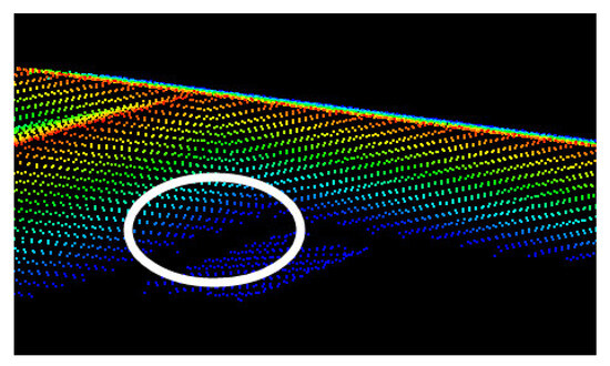
Figure 7.
An abrupt height change (the white circle) in one certain point’s neighborhood.
3.3. Extraction of Internal Feature Lines
The internal roof feature lines can be separated into three groups, normal ridge lines, oblique ridge lines and valley lines, as shown in Figure 1. Normal ridge lines are generally parallel or orthogonal to the main direction of the regular roof outlines, and those points within a certain distance to the corresponding normal ridge line have similar height values. Oblique ridge lines and valley lines are the intersection lines of two adjacent roof planes from top to bottom. The difference is that oblique ridge lines bulge outward, while valley lines are concave inward. In general, the end points of oblique ridge lines and valley lines should coincide with the end points of normal ridge lines or roof outlines. Thus, the accurate extraction of normal ridge lines is much helpful for the efficient extraction of oblique ridge lines and valley lines.
In this section, normal ridge lines are firstly extracted, followed by oblique ridge lines and valley lines through estimating the curvature variation of each point. Further, the intersection of each line or not should be estimated and improved to depict the internal features of roof structure accurately.
3.3.1. Normal Ridge Lines
This paper proposed a hill-climbing strategy to search for the points located in normal ridge lines. Begin with the edge points extracted in Section 3.2, and search for normal ridge points along the direction of the fastest gradient rise in one certain point’s neighborhood. The details are described as follows.
(1) Take each edge point as the beginning point. Climb up along the direction of the fastest gradient rise in ’s sphere neighborhood until the point with the local maximum height value determined. Add into the initial normal ridge point set .
(2) Region growing with height constraints. Take each in as a seed point. Find points with the absolute height difference to lower than an average height difference in ’s sphere neighborhood. Add into the expanding normal ridge point set . It is noteworthy that if one certain point p in cannot conduct region growing, p should be considered as an outlier and eliminated from .
(3) Similarly, region growing with height constraints is conducted for . Then, the final normal ridge point set can be formed.
(4) Separate the points in into several groups by analyzing the relationship between points. Two steps are used:
a. Combination. The points with overlapping neighbor points should belong to the same group.
b. Separation. This process should proceed for those normal ridge point sets with overlapping points after step (a), with the following two situations, as shown in Figure 8, where black points represent the normal ridge points and red dot lines are normal ridge lines.
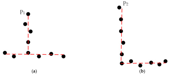
Figure 8.
Two situations for those normal ridge point sets with overlapping points: (a) internal overlapping and (b) end to end.
- ①
- Given a set of normal ridge points , and the two points with the farthest planar distance can be selected. Take one of these two points as the center of a circle, as shown in in (a) and in (b).
- ②
- Several lines passing through can be plotted, where and ranges from 0 to 175 degrees at intervals of 5 degrees. A total of 35 lines can be determined.
- ③
- For each line , the initial set of normal ridge points belongs to can be obtained by calculating the distance between each point and . If the distance is smaller than the average point spacing, the corresponding point is considered as an initial normal ridge point. Project all points in onto . Take as the beginning point, and calculate the distance between two adjacent points in one direction successively. If the distance is greater than twice the average point spacing (an empirical value), the remaining points that have not been calculated should be eliminated from . Then, can be determined.
- ④
- Among those lines passing through , a certain line with the most points should be selected. The final line can be fitted by the corresponding points using gradient descent method and those points should be labeled.
- ⑤
- For the remaining unlabeled points in S, repeat steps ① to ④ until the number of unlabeled points is fewer than 2. It is noteworthy that for the points located at the intersection area of two normal ridge lines, the reusing strategy is adapted to guarantee the completeness of each normal ridge line.
(5) Project each group of normal ridge points onto the corresponding line and the coarse coordinates of two end points can be obtained.
(6) In general, normal ridge lines should be parallel to one certain roof outline. For each normal ridge line , the outline with the minimum angle (smaller than 15 degrees) should be taken as the reference for normalizing .
(7) Due to the reusing strategy in step (4), the end points of two normal ridge lines should have intersected cannot be coincided. Then, the planar coordinates of the intersected point can be acquired by intersecting the two lines. Similar to the planar coordinates of the end point intersecting with a roof outline. Further, the height Z values of these end points use the same strategy in Section 3.2.2.
3.3.2. Oblique Ridge Lines and Valley Lines
The end points of oblique ridge lines and valley lines may (1) locate on an outline and (2) coincide with the end points of a normal ridge line or an outline. Then, for each roof point , the curvature value can be calculated using the following formula:
where are the eigenvalues of the covariance matrix composed of ’s sphere neighbor points. If is bigger than a threshold, can be considered as a candidate point and added into the set S. Detailed analysis for the threshold will be discussed in the experiment section. Separate points in S into several groups using the same strategy as the normal ridge points, and eliminate those groups with too few points. The end points should be differentiated into several categories and handled accordingly as follows:
(1) For each neighbor point set , if there are two or more outline end points with the same planar coordinates and different height values, the abrupt height change in Section 3.2.2 Figure 7 should be considered. Then, the corresponding outline should be completed. Firstly, add the outline end points with similar height values into . Label all points in and project them onto the corresponding outline and obtain the new end points. If the planar distance between the two end points belonging to two outlines is shorter than the sphere radius, the two outlines should be intersected to acquire the planar coordinates of the intersection point, while its height value is obtained using the inverse distance weighted average method for the five nearest neighbor points.
(2) For each remaining unlabeled neighbor point set :
- ①
- If there exists normal ridge points or outline points near to the corresponding end points, then the new end points of the corresponding feature line should be replaced by the end points of the determined normal ridge line or outline.
- ②
- If there are edge points and no end points of outlines, linear fitting is adapted for all points in . If one end point has been determined, translate the fitted line to pass through the determined end point. The other end point can be acquired by intersection.
- ③
- Otherwise, all points are used to fit a feature line and projected onto the line to obtain the corresponding end points.
4. Experiments and Discussion
Figure 9 shows the extraction results of initial roof edge points. It is noteworthy that the edge points extracted by our proposed algorithm are dense and consecutive, which is helpful for the subsequent extraction of roof outlines. Figure 10 shows the extraction results of initial roof outlines, where yellow points represent the edge points and red lines represent the outlines. Seen from Figure 10, the two adjacent outlines are generally orthogonal to each other for regular building roofs on XOY projection plane. However, it is likely that there are several special outlines, as shown in white circles in (b). In addition, the real corner points that should be in the white circles in (f) cannot be extracted due to the space resolution of the original point clouds.
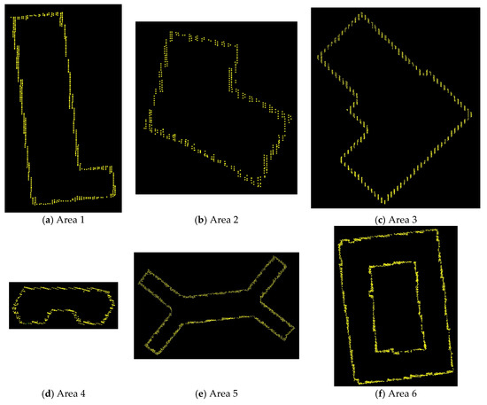
Figure 9.
The extraction results of initial roof edge points.
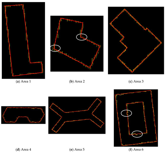
Figure 10.
The initial roof outlines (red lines) for six test data.
Further, the initial outlines cannot include all edge points, as shown in Figure 10. But these outside edge points should belong to the roof, which means that the initial outlines are smaller than its real range. Hence, coarse roof outlines are refined by normalization and expansion proposed in Section 3.2.2. The refined roof outlines are shown in Figure 11, where (a) to (c) display the refined outlines and the original point clouds for Areas 1 to 3 on the corresponding images repeatedly, while (d) to (f) show the results of Areas 4 to 6. Seen from Figure 11f, it is interesting that the inner outline (like a courtyard) can also be extended to the accurate direction using the proposed method.
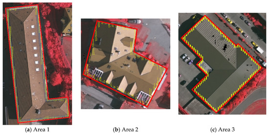
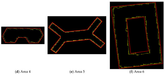
Figure 11.
The refined roof outlines (red lines) for six test data.
Due to lack of the corresponding orthophoto in Alashan, Areas 4 to 6 cannot conduct quantitative evaluation. It is noteworthy that the proposed method is able to obtain various types of roof outlines, including irregular roofs (Figure 11d,e) and the roof with a courtyard (Figure 11f), which achieves a promising visual results. Table 1 lists the results for 22 corner points in Areas 1 to 3 using mean square error of coordinates. The real coordinates of these corner points are measured manually using LPS module in ERDAS 2015 software, according to the orthophoto provided by ISPRS.

Table 1.
Mean square error of coordinates for 22 corner points in Areas 1 to 3 (units: meters).
It is noteworthy that Areas 1 to 3 include the common types of internal roof feature lines. Hence, test data in this section use Areas 1 to 3. Figure 12 shows the extraction process of normal ridge lines using the proposed algorithm in Section 3.3.1. Figure 12a–c display the initial normal ridge lines, where red points are normal ridge points and white points are roof data. Yellow lines are the initial normal ridge lines after linear fitting, which are not parallel to the corresponding outlines. Figure 12d–f display normal ridge lines after normalization with the corresponding orthophoto and outlines. These final normal ridge lines are almost overlapped with the corresponding positions on the images. However, Area 2 performs not well due to complicated roof structure. For Area 2, the two main normal ridge lines are extracted accurately, but there are some deviations for those short ones. The reasons may include two aspects: insufficient data density and complexity of the structure. In general, the ancillary facilities are small and short. Their extraction results are easy to be affected by their surroundings. Further, the roof structure of Area 2 is very complicated and its corresponding point data are discrete with low flatness. This results in limited normal ridge points being extracted for each line. It is a pity that these short and complicated normal ridge lines cannot be extracted accurately under the existing conditions. Hence, the following oblique ridge lines and valley lines cannot be extracted accurately too, which results in the necessary manual correction.
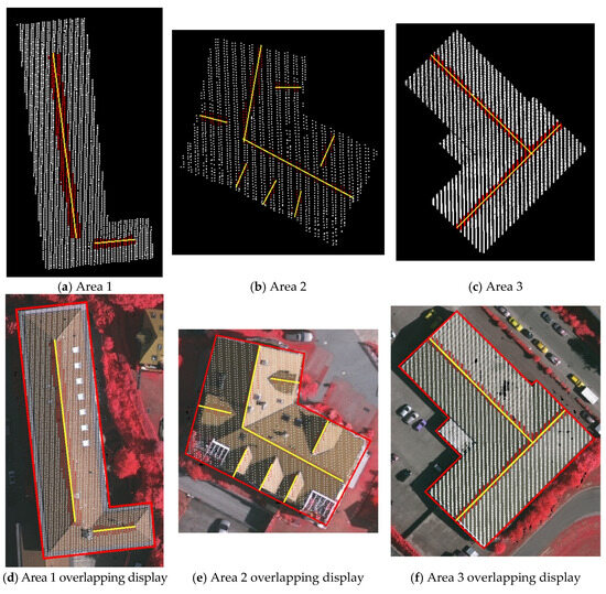
Figure 12.
The extraction results of normal ridge lines for Areas 1 to 3, where (a–c) display the initial normal ridge lines and (d–f) display normal ridge lines after normalization with the corresponding orthophoto and outlines.
For oblique ridge lines and valley lines, the curvature value of each point is adopted as an evaluation indicator. In this section, this paper conducts several groups of experiments for determining the thresholds of curvature for different data, in order to find a suitable and rational threshold for each data. The results are shown in Figure 13, Figure 14 and Figure 15. It is noteworthy that when the threshold of curvature decreases gradually, more extracted points can be obtained; otherwise, when the threshold is too small, the points are extracted disorderly, which makes it difficult to extract feature lines efficiently. Seen from these three figures, the accessories in Area 2 are too various, which leads to unclear distinguishing boundaries of different groups of points. Thus, oblique ridge lines and valley lines in Area 2 are hard to extract accurately. In addition, the roof structures of Area 1 and Area 3 are relatively simple and each feature line is extracted separately, which can achieve promising results of extracting the subsequent feature lines.
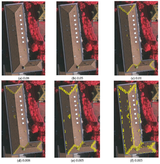
Figure 13.
Variation of the extracted points belonging to oblique ridge lines and valley lines using different thresholds of curvature for Area 1 (the maximum curvature is 0.14 m and the average value is 0.006 m).
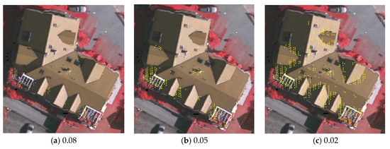
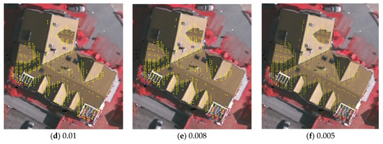
Figure 14.
Variation of the extracted points belonging to oblique ridge lines and valley lines using different thresholds of curvature for Area 2 (the maximum curvature is 1 m and the average value is 0.023 m).
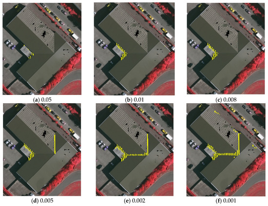
Figure 15.
Variation of the extracted points belonging to oblique ridge lines and valley lines using different thresholds of curvature for Area 3 (the maximum curvature is 0.09 m and the average value is 0.001 m).
According to Figure 13 and Figure 15, the feature points can be extracted clearly and completely with few noise points if the threshold of curvature is twice the average curvature, when the roof structure is relatively simple. Figure 16 shows the initial extraction results of oblique ridge lines and valley lines for three sets of data (yellow solid lines). As mentioned above, visual results of Area 1 and Area 3 are very promising. In the white circle in Figure 16c, there is an abrupt height change as described in Figure 7. From the view of three dimensions, the two yellow lines should not be omitted. However, many related research mainly focus on the external outlines. And the two outlines are supplemented, which is consistent with the objective fact. It should be noted that, due to the unsatisfied extraction results of feature points, the internal feature lines are extracted wrongly except two long feature lines, which acquires necessary manual correction. Figure 17 shows the final results after manual correction.
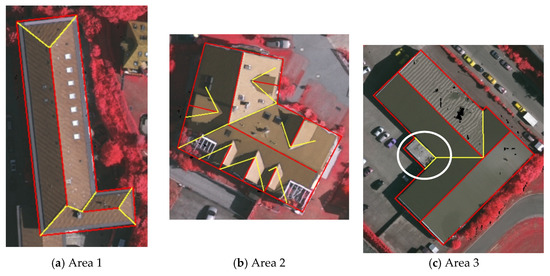
Figure 16.
The initial extraction results of oblique ridge lines and valley lines for different test data from Areas 1 to 3.
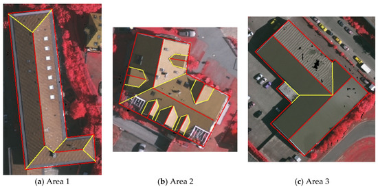
Figure 17.
The final results of roof feature lines after manual correction.
5. Conclusions
This paper proposed a new outside-in strategy to extract roof feature lines from the original airborne LiDAR data, including outlines, normal ridge lines, oblique normal ridge lines and valley lines successively. For roof outlines, a grid-based method is adopted to search for the initial edge points. Experimental results show that this method is fast and efficient, and the extracted edge points are dense and consecutive. Subsequently, a grouping strategy based on the geometric characteristics of LiDAR data is utilized to separate those initial edge points into several groups, and the gradient descent method is used to fit the coarse roof outlines. Then, according to the general knowledge of roof structure [5,8,33], the roof outlines can be refined by normalization and expansion. After extracting the roof outlines accurately, those internal feature lines should be acquired, which means that the precision of roof outlines is crucial to extract the subsequent internal feature lines. For normal ridge lines, a hill-climbing strategy is adopted, taking each edge point as the beginning point and searching for the normal ridge points along the direction of the fastest gradient rise. Then, according to the corresponding outlines, the normal ridge lines can be normalized by a region-growing strategy with height constraints and a group fitting method. For oblique normal ridge lines and valley lines, their end points are determined by calculating the curvature value. Further, the relationship between the threshold of the curvature and number of feature points is also determined through several experiments. The results show that the proposed procedure of extracting roof feature lines can acquire the accurate coordinates of end points efficiently and automatically, especially for roofs with a relatively simple structure. This paper provides a novel vision to extract roof feature lines from the geometric characteristics of LiDAR data itself. However, for roofs with a complicated structure (like Area 2 in this paper), data density is still a tough factor of high-accuracy extracting internal feature lines. In addition, there are several parameters, both in the extraction of outlines and internal feature lines, that need presetting manually. Our future work will focus on the automatic determination of these parameters according to data density and improving extraction precision with various data density.
Author Contributions
Conceptualization, Z.C.; methodology, Z.C.; software, H.M.; validation, Z.C.; formal analysis, Z.C.; investigation, Z.C. and L.Z.; resources, Z.C.; data curation, Z.C.; writing—original draft preparation, Z.C.; writing—review and editing, H.M. and L.Z.; visualization, Z.C.; supervision, H.M. and L.Z.; project administration, Z.C.; funding acquisition, Z.C. All authors have read and agreed to the published version of the manuscript.
Funding
This research was funded by the Tianjin Key Laboratory of Rail Transit Navigation Positioning and Spatio-temporal Big Data Technologh (TKL2023B13 and TKL2023B15), the National Natural Science Foundation of China (41601504), the Education Commission of Hubei Province of China (Q20202801), and the Ph.D. Research Start-up Foundation of Hubei University of Science and Technology (L07903/170428).
Data Availability Statement
The data presented in this study are openly available in reference [33].
Acknowledgments
The test datasets were provided by the International Society for Photogrammetry and Remote Sensing (ISPRS) Working Group and OpenTopography. Authors would like to thank them and anonymous reviewers for their constructive comments for the manuscript.
Conflicts of Interest
The authors declare no conflict of interest.
References
- Du, S.J.; Zhang, Y.S.; Zou, Z.R.; Xu, S.H.; He, X.; Chen, S.Y. Automatic building extraction from LiDAR data fusion of point and grid-based features. ISPRS-J. Photogramm. Remote Sens. 2017, 130, 294–307. [Google Scholar] [CrossRef]
- Yang, B.S.; Huang, R.G.; Li, J.P.; Tian, M.; Dai, W.X.; Zhong, R.F. Automated Reconstruction of Building LoDs from Airborne LiDAR Point Clouds Using an Improved Morphological Scale Space. Remote Sensing 2017, 9, 14. [Google Scholar] [CrossRef]
- Salehi, A.; Mohammadzadeh, A. Building Roof Reconstruction Based on Residue Anomaly Analysis and Shape Descriptors from Lidar and Optical Data. Photogramm. Eng. Remote Sens. 2017, 83, 281–292. [Google Scholar] [CrossRef]
- Griffiths, D.; Boehm, J. Improving public data for building segmentation from Convolutional Neural Networks (CNNs) for fused airborne lidar and image data using active contours. ISPRS-J. Photogramm. Remote Sens. 2019, 154, 70–83. [Google Scholar] [CrossRef]
- Sampath, A.; Shan, J. Building boundary tracing and regularization from airborne lidar point clouds. Photogramm. Eng. Remote Sens. 2007, 73, 805–812. [Google Scholar] [CrossRef]
- Sun, S.H.; Salvaggio, C. Aerial 3D Building Detection and Modeling from Airborne LiDAR Point Clouds. IEEE J. Sel. Top. Appl. Earth Obs. Remote Sens. 2013, 6, 1440–1449. [Google Scholar] [CrossRef]
- dos Santos, R.C.; Galo, M.; Carrilho, A.C. Extraction of Building Roof Boundaries from LiDAR Data Using an Adaptive Alpha-Shape Algorithm. IEEE Geosci. Remote Sens. Lett. 2019, 16, 1289–1293. [Google Scholar] [CrossRef]
- Feng, M.L.; Zhang, T.G.; Li, S.C.; Jin, G.Q.; Xia, Y.J. An improved minimum bounding rectangle algorithm for regularized building boundary extraction from aerial LiDAR point clouds with partial occlusions. Int. J. Remote Sens. 2020, 41, 300–319. [Google Scholar] [CrossRef]
- Yang, J.T.; Kang, Z.Z.; Akwensi, P.H. A Label-Constraint Building Roof Detection Method from Airborne LiDAR Point Clouds. IEEE Geosci. Remote Sens. Lett. 2021, 18, 1466–1470. [Google Scholar] [CrossRef]
- Kaplan, G.; Comert, R.; Kaplan, O.; Matci, D.K.; Avdan, U. Using Machine Learning to Extract Building Inventory Information Based on LiDAR Data. ISPRS Int. J. Geo-Inf. 2022, 11, 517. [Google Scholar] [CrossRef]
- Dey, E.K.; Awrangjeb, M.; Stantic, B. Outlier detection and robust plane fitting for building roof extraction from LiDAR data. Int. J. Remote Sens. 2020, 41, 6325–6354. [Google Scholar] [CrossRef]
- Wang, J.; Qin, Q.; Chen, L.; Ye, X.; Qin, X.; Wang, J.; Chen, C. Automatic building extraction from very high resolution satellite imagery using line segment detector. In Proceedings of the 2013 IEEE International Geoscience and Remote Sensing Symposium-IGARSS, Melbourne, VIC, Australia, 21–26 July 2013; pp. 212–215. [Google Scholar]
- Chen, K.; Zou, Z.; Shi, Z. Building Extraction from Remote Sensing Images with Sparse Token Transformers. Remote Sens. 2021, 13, 4441. [Google Scholar] [CrossRef]
- Baltsavias, E.P. Airborne Laser Scanning: Existing Systems and Firms and Other Resources. ISPRS-J. Photogramm. Remote Sens. 1999, 54, 164–198. [Google Scholar] [CrossRef]
- Li, L.; Song, N.; Sun, F.; Liu, X.Y.; Wang, R.S.; Yao, J.; Cao, S.S. Point2Roof: End-to-end 3D building roof modeling from airborne LiDAR point clouds. ISPRS-J. Photogramm. Remote Sens. 2022, 193, 17–28. [Google Scholar] [CrossRef]
- Sadeq, H.A.J. Building Extraction from Lidar Data Using Statistical Methods. Photogramm. Eng. Remote Sens. 2021, 87, 33–42. [Google Scholar] [CrossRef]
- Sampath, A.; Shan, J. Segmentation and Reconstruction of Polyhedral Building Roofs from Aerial Lidar Point Clouds. IEEE Trans. Geosci. Remote 2010, 48, 1554–1567. [Google Scholar] [CrossRef]
- Galvanin, E.A.D.; Dal Poz, A.P. Extraction of Building Roof Contours from LiDAR Data Using a Markov-Random-Field-Based Approach. IEEE Trans. Geosci. Remote Sens. 2012, 50, 981–987. [Google Scholar] [CrossRef]
- Cao, R.J.; Zhang, Y.J.; Liu, X.Y.; Zhao, Z.Z. 3D building roof reconstruction from airborne LiDAR point clouds: A framework based on a spatial database. Int. J. Geograph. Inf. Sci. 2017, 31, 1359–1380. [Google Scholar] [CrossRef]
- Lee, J.; Han, S.; Byun, Y.; Kim, Y. Extraction and Regularization of Various Building Boundaries with Complex Shapes Utilizing Distribution Characteristics of Airborne LIDAR Points. ETRI J. 2011, 33, 547–557. [Google Scholar] [CrossRef]
- Wang, R.S.; Hu, Y.; Wu, H.Y.; Wang, J. Automatic extraction of building boundaries using aerial LiDAR data. J. Appl. Remote Sens. 2016, 10, 016022. [Google Scholar] [CrossRef]
- Zhao, Z.Z.; Duan, Y.S.; Zhang, Y.J.; Cao, R.J. Extracting buildings from and regularizing boundaries in airborne lidar data using connected operators. Int. J. Remote Sens. 2016, 37, 889–912. [Google Scholar] [CrossRef]
- Sreevalsan-Nair, J.; Jindal, A.; Kumari, B. Contour Extraction in Buildings in Airborne LiDAR Point Clouds Using Multiscale Local Geometric Descriptors and Visual Analytics. IEEE J. Sel. Top. Appl. Earth Obs. Remote Sens. 2018, 11, 2320–2335. [Google Scholar] [CrossRef]
- Santos, R.C.d.; Pessoa, G.G.; Carrilho, A.C.; Galo, M. Automatic Building Boundary Extraction from Airborne LiDAR Data Robust to Density Variation. IEEE Geosci. Remote Sens. Lett. 2022, 19, 1–5. [Google Scholar] [CrossRef]
- Li, Y.; Wu, H.; An, R.; Xu, H.; He, Q.; Xu, J. An improved building boundary extraction algorithm based on fusion of optical imagery and LIDAR data. Optik 2013, 124, 5357–5362. [Google Scholar] [CrossRef]
- Cheng, L.G.; Chen, J.; Han, X.P. Building Boundary Extraction from High Resolution Imagery and Lidar Data. Int. Arch. Photogramm. Remote Sens. Spat. Inf. Sci. 2008, 37, 693–698. [Google Scholar]
- Sun, Y.; Zhang, X.C.; Zhao, X.Y.; Xin, Q.C. Extracting Building Boundaries from High Resolution Optical Images and LiDAR Data by Integrating the Convolutional Neural Network and the Active Contour Model. Remote Sens. 2018, 10, 1459. [Google Scholar] [CrossRef]
- Akbulut, Z.; Özdemir, S.; Acar, H.; Karsli, F. Automatic Building Extraction from Image and LiDAR Data with Active Contour Segmentation. J. Indian Soc. Remote 2018, 46, 2057–2068. [Google Scholar] [CrossRef]
- Awrangjeb, M. Using point cloud data to identify, trace, and regularize the outlines of buildings. Int. J. Remote Sens. 2016, 37, 551–579. [Google Scholar] [CrossRef]
- Zhang, D.; Du, P. 3D Building Reconstruction from Lidar Data Based on Delaunay TIN Approach; SPIE: St. Bellingham, WA, USA, 2011; Volume 8286. [Google Scholar]
- Edelsbrunner, H.; Kirkpatrick, D.; Seidel, R. On the shape of a set of points in the plane. IEEE Trans. Inf. Theory 1983, 29, 551–559. [Google Scholar] [CrossRef]
- Hofman, P.; Potůčková, M. Comprehensive approach for building outline extraction from LiDAR data with accent to a sparse laser scanning point cloud. Geoinform. FCE CTU 2017, 16, 91–102. [Google Scholar] [CrossRef]
- Cramer, M. The DGPF-test on digital airborne camera evaluation—Overview and test design. Photogramm.-Ernerkundung-Geoinf. 2010, 2010, 73–82. [Google Scholar] [CrossRef] [PubMed]
Disclaimer/Publisher’s Note: The statements, opinions and data contained in all publications are solely those of the individual author(s) and contributor(s) and not of MDPI and/or the editor(s). MDPI and/or the editor(s) disclaim responsibility for any injury to people or property resulting from any ideas, methods, instructions or products referred to in the content. |
© 2023 by the authors. Licensee MDPI, Basel, Switzerland. This article is an open access article distributed under the terms and conditions of the Creative Commons Attribution (CC BY) license (https://creativecommons.org/licenses/by/4.0/).