Evaluation of Original and Water Stress-Incorporated Modified Weather Research and Forecasting Vegetation Photosynthesis and Respiration Model in Simulating CO₂ Flux and Concentration Variability over the Tibetan Plateau

Abstract

Terrestrial carbon fluxes are crucial to the global carbon cycle. Quantification of terrestrial carbon fluxes over the Tibetan Plateau (TP) has considerable uncertainties due to the unique ecosystem and climate and scarce flux observations. This study evaluated our recent improvement of terrestrial flux parameterization in the weather research and forecasting model coupled with the vegetation photosynthesis and respiration model (WRF-VPRM) in terms of reproducing observed net ecosystem exchange (NEE), gross ecosystem exchange (GEE), and ecosystem respiration (ER) over the TP. The improvement of VPRM relative to the officially released version considers the impact of water stress on terrestrial fluxes, making it superior to the officially released model due to its reductions in bias, root mean square error (RMSE), and ratio of standard deviation (RSD) of NEE to 0.850 μmol·m⁻²·s⁻¹, 0.315 μmol·m⁻²·s⁻¹, and 0.001, respectively. The improved VPRM also affects GEE simulation, increasing its RSD to 0.467 and decreasing its bias and RMSE by 1.175 and 0.324 μmol·m⁻²·s⁻¹, respectively. Furthermore, bias and RMSE for ER were lowered to −0.417 and 0.954 μmol·m⁻²·s⁻¹, with a corresponding increase in RSD by 0.6. The improved WRF-VPRM simulation indicates that eastward winds drive the transfer of lower CO₂ concentrations from the eastern to the central and western TP and the influx of low-concentration CO₂ inhibits biospheric CO₂ uptake. The use of an improved WRF-VPRM in this study helps to reduce errors, improve our understanding of the role of carbon flux cycle over the TP, and ultimately reduce uncertainty in the carbon flux budget.

1. Introduction

Carbon fluxes and CO₂ concentrations in terrestrial ecosystems received increasing attention due to the uncertainties caused by global warming in recent years [1]. Alterations in terrestrial ecosystem carbon sinks and sources influence atmospheric CO₂ concentrations, thereby modulating the global carbon cycle. Carbon sources and sinks across diverse vegetation types and eco-climatic zones were examined using various methods, such as inventories [2,3,4,5], in situ observations [6,7,8], satellite inversions [9,10,11], spaceborne observations [12,13,14], and model simulations [15,16,17,18,19]. Under the conditions of long-term warming, the carbon assimilation capacity on the Tibetan Plateau (TP) increased [20,21,22]. However, due to the release of soil carbon from permafrost degradation [23,24] and the frequent ecosystem disruption caused by extreme events [25,26], obtaining reliable information on changes in carbon flux is particularly important. Hence, utilizing model simulations is imperative for the in-depth exploration of the vulnerable TP. The light use efficiency model emerged as the primary approach for predicting carbon flux, owing to the limited observation range of eddy covariance systems and the influence of cloud microphysics on satellite data.

Previous studies employing physiological processes and empirical equations demonstrated a link between CO₂ fluxes and both temperature [10] and photosynthesis [27]; however, an evident degree of uncertainty that needs to be further examined persists. Concurrently, vegetation growth also greatly influences CO₂ flux. The enhanced vegetation index (EVI), calculated using near IR (NIR) and red and blue band reflectance [28], has lower sensitivity to soil background reflectance and residual atmospheric contamination; therefore, it can indicate vegetation changes more effectively than the normalized difference vegetation index [29]. Churkina et al. [30] observed that EVI is closely linked to the carbon sink period and used it to estimate large-scale net ecosystem exchange (NEE) using remote sensing data. The fraction of absorbed incident photosynthetically active radiation (FAPAR) is a constant approximated by EVI and is used to estimate light use efficiency [31]. EVI was incorporated into the temperature and greenness model [32], canopy reflectance model [33], vegetation photosynthesis model [29], and weather research and forecasting model coupled with the vegetation photosynthesis and respiration model (WRF-VPRM) [34,35] to simulate carbon flux. Furthermore, EVI was shown to exhibit strong correlations with GPP and NEE across diverse regions [36,37,38]. Meanwhile, since WRF-VPRM is a coupled model, it enables the study of the impacts and responses of climate on carbon flux [39,40]. In contrast, traditional ecological models such as ORCHIDEE [41,42] and BIOME-BGC [43,44] typically focus solely on the influence of climate on flux, making WRF-VPRM widely applicable.

The WRF-VPRM used to stimulate CO₂ fluxes was validated and analyzed using data derived from 12 North American sites [34,35]. This process enabled parametric adjustments, leading to robust results with high spatiotemporal resolution [35]. The model was recognized for its capability to capture vertical profiles and fronts, as demonstrated by applications in the United States [40]. Moreover, the WRF-VPRM consistently simulated carbon flux in relation to localized climate changes observed along the European coast [34]. Moreover, the model can replicate diurnal and seasonal variations in carbon flux within planetary boundary layers [45] and valleys [46]. Despite several studies providing information on the carbon cycle, substantial uncertainty regarding the factors influencing this cycle persists. Moreover, the relationship among vegetation respiration, photosynthesis, and water stress [39,47,48,49,50] remains ambiguous.

The influence of water stress on gross ecosystem exchange (GEE) and ecosystem respiration (ER) is notably stronger than the impact of temperature in alpine meadows [50]. Additionally, water stress can induce a shift from carbon sinks to weak carbon sources, as observed in Europe [15]. Lee et al. [48] highlighted the effect of water stress on carbon cycling in pine forests in semi-arid regions, using WRF-VPRM, which optimized water stress. Although the effects of temperature, photosynthesis, EVI, and water stress on carbon flux were extensively studied across diverse ecosystems [51,52,53,54,55], the relationship between carbon flux and CO₂ concentration in the unique TP ecosystem requires further comprehensive investigation.

Owing to its high elevation and harsh natural environmental conditions, the TP has few observation sites, particularly carbon flux observation sites [52]. Satellite remote sensing products are critical for studying local changes in carbon fluxes; however, these products exhibit substantial biases in the TP due to high elevation and extensive cloud coverage [56]. Therefore, the WRF-VPRM faces significant challenges in simulating carbon fluxes at high altitudes and in unique natural environments.

This study reconstructs realistic carbon fluxes and surface CO₂ concentrations over the TP using WRF-VPRM by considering water stress, followed by an evaluation and analysis of the results. This quantification of CO₂ concentration and flux changes at individual sites across the TP paves the way for comprehensive investigations into the mutual interactions between carbon flux and regional climate over the TP. The remainder of the manuscript is organized as follows: Section 2 introduces the data used, the study site, and the WRF-VPRM. Section 3 evaluates and analyzes daily growing season diurnal variations, and cumulative changes in surface carbon flux in major TP ecosystems. The changes in CO₂ concentrations caused by advection, which are reflected by changes in carbon fluxes, typically presumed to be vertical, were then investigated. Section 4 discusses the main factors contributing to improving the WRF-VPRM and the existing limitations. Finally, the conclusions are presented in Section 5.

2. Methods

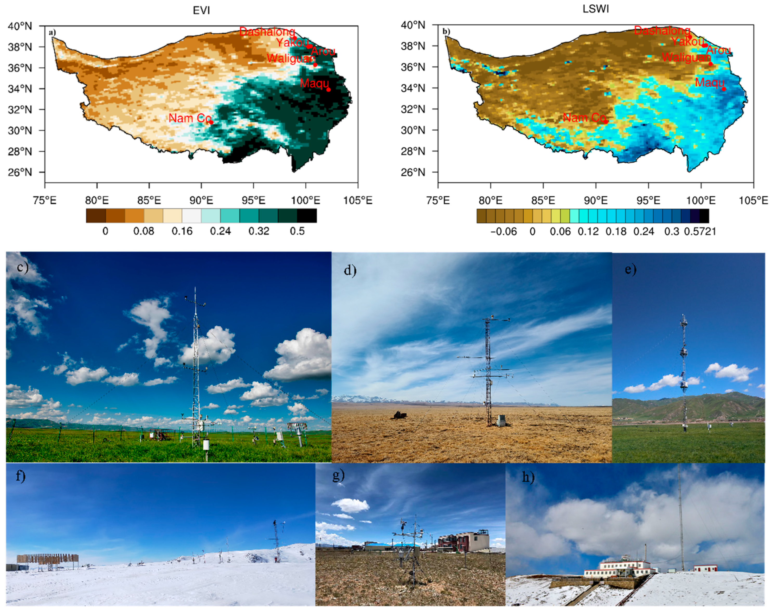
2.1. In Situ and Satellite Observations

The TP (average elevation: 4000 m) covers approximately 2,500,000 km² of Southwest China. In this study, data sourced from in situ observations at six sites (Maqu, Yakou, Dashalong, Arou, Nam Co, and Mt.Waliguan) on the TP [57,58,59] were used to validate the proposed WRF-VPRM (

Table 1. Geographic characteristics of the sites.

Name	Site	Altitude (m)	Substrate
Maqu	33.8975°N, 102.1619°E	3423	Kobresia tibetica and K. humilis
Yakou	38.0142°N, 100.2421°E	4148	Alpine grassland
Dashalong	38.8399°N, 98.9406°E	3739	Swampy alpine meadows
Arou	38.0473°N, 100.4643°E	3033	Alpine grassland
Nam CO	30.7667°N, 90.95°E	4730	K. pygmaea and alpine steppe
Mt. Waliguan	36.28°N, 100.9°E	3810	Arid and semi-arid grasslands, tundra, and deserts

). Observations covering several micrometeorological variables in conjunction with eddy covariance measurements were conducted at these sites, as described by Shang et al. [60] and Liu et al. [58]. Additionally, in this study, leveraged CO₂ concentration data were retrieved from the Waliguan Atmospheric Background Station as part of the World Data Centre for Greenhouse Gases project. CO₂ flux data from Nam Co [61] were also utilized to evaluate the efficacy of the WRF-VPRM in accurately simulating carbon fluxes.

Given the inherent sensitivity of eddy covariance towers to measuring carbon flux and the potential for environmental disturbances, a rigorous data processing approach was employed for observations, as outlined by Shang et al. [60]. Raw flux data logged at 10 Hz from the eddy covariance instrumentation were processed using EddyPro software (LI-COR Biosciences, Lincoln, NE, USA) and subjected to meticulous quality control. The data were classified into growing and non-growing season subsets, based on temperature thresholds of 5 °C [62,63], while ensuring maximal retention of changes in data. Subsequent data filtration procedures were implemented to eliminate data entries that exceeded the average observation range for any of the three variables (sensible and latent heat and carbon flux), corresponded to the carbon flux observations during rainfall, were assigned quality grades above 1, and represented instances of low wind speeds at night. To fill data gaps, a combination of nonlinear regression, the lookup table method, and mean diurnal variation was applied, with the window size varying from 7 to 30 days based on site-specific data conditions. Specifically, following linear interpolation of available data points around missing time intervals, a 2-day window before and after the missing time point was selected for averaging. Subsequently, the lookup table method was applied to address data gaps exceeding 30 days, using temperature, radiation, and carbon flux availability as criteria for segmenting the missing periods for environmental comparisons. Finally, nonlinear interpolation was employed to address gaps lasting up to 10 consecutive days. The optimal window size, initially set at 7 days, was adjusted to up to 30 days based on data quality. According to the method described by Nieberding et al. [61], drift correction of the surface CO₂ concentration due to the systematic deviation of the flux tower was performed. To prevent short-term data anomalies, this method adopts the change in the median and uses the multi-period trigonometric function to reconstruct the background value for drift correction.

Additionally, the EVI product, as part of the MOD09a1 Collection 6 from the Moderate Resolution Imaging Spectroradiometer (MODIS) satellite, was utilized. The EVI data offer a spatial resolution of 500 m and are updated on an 8-day temporal scale [64].

2.2. Description of the WRF-VPRM

VPRM calculates terrestrial CO₂ flux at each time step and transmits it to the WRF meteorological field to simulate CO₂ concentrations [34,35,40,45,65]. In this study, the initial and boundary conditions of CO₂ concentrations were obtained from CarbonTracker (https://www.esrl.noaa.gov/gmd/ccgg/carbontracker/, (accessed on 17 September 2019)). The National Center for Environmental Prediction provided the initial and boundary conditions for meteorological variables [66]. EVI was obtained from MODIS, and a 0.1° × 0.1° anthropogenic emission inventory was supplied by the Open-source Data Inventory for Anthropogenic CO₂. The resulting model output included 48 vertical layers and exhibited a horizontal resolution of 20 km. EVI decreased from east to west, with the Maqu site located in the high EVI area and the Nam Co and Dashalong sites located on the edge of the high-value area (Figure 1a). Compared with its original version, the modified WRF-VPRM primarily improved the simulation accuracy by incorporating the effects of EVI and water stress in ER and GEE calculations. Moreover, the WRF-VPRM revealed changes in ecosystem CO₂ fluxes by simulating the following functions containing specific vegetation-related parameters [35,39]:

$$NEE=ER+GEE,$$

(1)

$$ER=\alpha ·EVI+A+B·T+C·T^2$$

(2)

$$ER={\gamma }_1+{\gamma }_2·T$$

(3)

$$GEE=\beta ·W_{scale}·T_{scale}·P_{scale}·{FAPAR}_{PAV}·PAR·{\left(1+PAR·{{PAR}_0}^{-1}\right)}^{-1}$$

(4)

$$A={\gamma }_1+k_1·W_{scale}$$

(5)

$$B={\gamma }_2+k_2·W_{scale}$$

(6)

$$C={\gamma }_3+k_3·W_{scale}$$

(7)

where NEE is the net ecosystem exchange, ER is the sum of autotrophic and heterotrophic respiration, and GEE represents vegetation productivity (Equations (1), (2), and (4)). α, β, γ (γ₁, γ₂, and γ₃), and k (k₁, k₂, and k₃) are parameters pertaining to the specific vegetation types (Equations (5)–(7)). The effects of W_scale, T_scale, and P_scale on GEE (Equation (4)) represent the changes in temperature stress (Equation (12)), water stress (Equations (8) and (9)), and phenology (Equation (11)), respectively. FAPAR_PAV is the fraction of photosynthetically active radiation that can be approximately replaced by EVI, whereas PAR₀ is the half-saturation value (Equation (4)). The original ER function contains only the primary linear term for temperature (Equation (3)). An improved terrestrial respiration parameterization in the VPRM was developed by incorporating EVI, water stress scaling factor, and quadratic dependence on surface air temperature (Equation (2)).

$$W_{scale\left(GEE\right)}=1-\left({LSWI}_{max}-LSWI\right)·{\left(1+{LSWI}_{max}\right)}^{-1}$$

(8)

$$W_{scale\left(RE\right)}=1-\left({LSWI}_{max}-LSWI\right)·{\left({LSWI}_{max}-{LSWI}_{min}\right)}^{-1}$$

(9)

$$LSWI=1-2·{\rho }_{SWIR}·{\left({\rho }_{NIR}+{\rho }_{SWIR}\right)}^{-1}$$

(10)

$$P_{scale}=\left(1+LSWI\right)·2^{-1}$$

(11)

$$T_{scale}=1-{\left(T-T_{opt}\right)}^2·{\left[{\left(T-T_{opt}\right)}^2-\left(T-T_{min}\right)·\left(T-T_{max}\right)\right]}^{-1}$$

(12)

The original WRF-VPRM algorithm uniformly applied water stress to both the GEE and ER (Equation (8)). The modified WRF-VPRM distinguished the effects of water stress on photosynthesis and respiration (Equations (8) and (9)), following the methodology of Hu et al. [39]. The land surface water index (LSWI) is computed as a normalized value for NIR and short-wave radiation and indicates phenological patterns [29] (Equation (10)). The spatial distribution of the LSWI was similar to that of EVI (Figure 1b). The T_opt, T_max, and T_min values of different vegetation types represented the optimum, maximum, and minimum temperatures (Equation (12)) for photosynthesis, respectively, from previous studies [35,39].

$$T_{new}=T_a·T_{scale}-T_{crit}\left(T_{scale}-1\right)$$

(13)

The temperature was adjusted to respond as much as possible to low-temperature conditions (Equation (13)) in cases where vegetation did not survive, but respiration persisted; additionally, low temperatures at night without respiration were considered “pseudo-death” when the air temperature (T_a) was below the threshold (T_crit). The parameters in the original model were obtained from Li et al. [18] and those in the improved model were obtained from Hu et al. [39].

2.3. Analytical Method

To quantify the difference between the WRF-VPRM simulations and observations, four statistical features were used at each site: bias, root mean square error (RMSE), correlation coefficient (r), and the ratio of standard deviation (RSD). These were calculated as follows:

$$\mathrm{b}\mathrm{i}\mathrm{a}\mathrm{s}=\frac{1}{\mathrm{N}}\sum _{i=1}^N\left(M_i-O_i\right)$$

(14)

$$RMSE={\left(\frac{1}{N-1}\sum _{i=1}^N{\left(M_i-O_i\right)}^2\right)}^{\frac{1}{2}}$$

(15)

$$r=\frac{\frac{1}{N}\sum _{i=1}^N\left(M_i-\overline{M}\right)\left(O_i-\overline{O}\right)}{\sqrt{\frac{1}{N}\sum _{i=1}^N{\left(M_i-\overline{M}\right)}^2}\sqrt{\frac{1}{N}\sum _{i=1}^N{\left(O_i-\overline{O}\right)}^2}}$$

(16)

$$RSD=\frac{\left|\sqrt{\frac{1}{N-1}\sum _{i=1}^N{\left(M_i-\overline{M}\right)}^2}-\sqrt{\frac{1}{N-1}\sum _{i=1}^N{\left(O_i-\overline{O}\right)}^2}\right|}{\sqrt{\frac{1}{N-1}\sum _{i=1}^N{\left(O_i-\overline{O}\right)}^2}}$$

(17)

where $M_i$ and $O_i$ are the simulated and observed values, respectively, $\overline{M}$ and $\overline{O}$ are the averages of the simulated and observed values, respectively, and N is the number of days for comparison.

3. Results

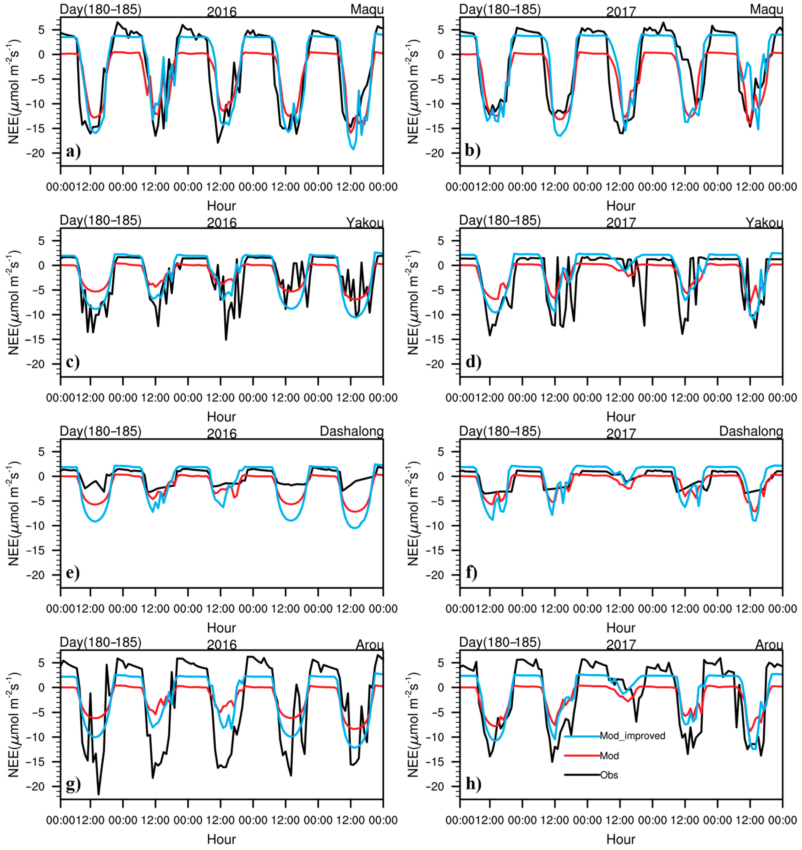
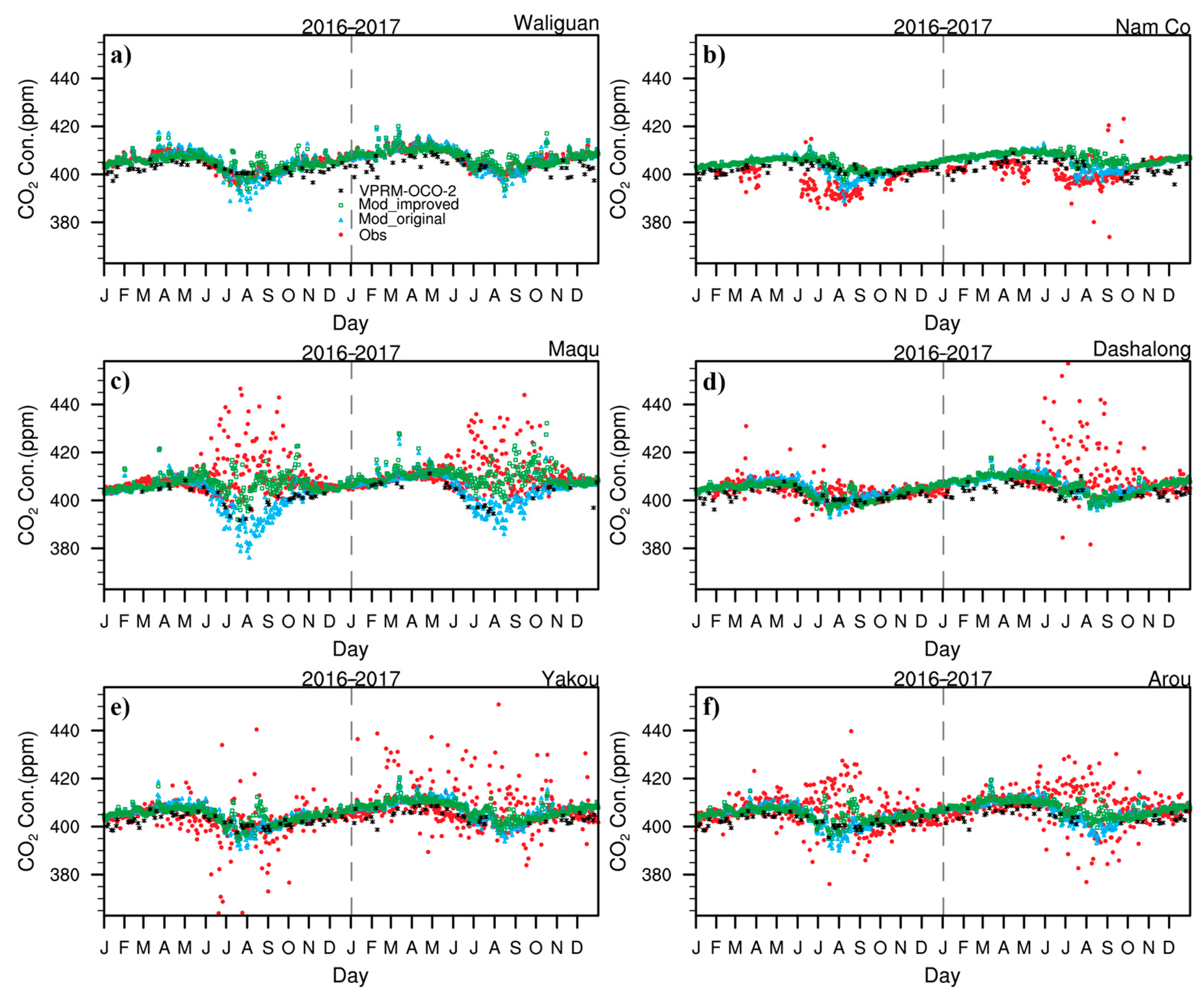
3.1. Seasonal Variations in CO₂ Fluxes and Hourly Variations in NEE and CO₂ Concentrations

Initially, the annual variations in NEE, GEE and ER were evaluated across four sites, i.e., Maqu, Dashalong, Arou, and Nam Co (Figure 2, Figure 3 and Figure 4). At Maqu, a negative daily mean NEE was observed from mid-April to late October (Figure 2a). The daily mean NEE peaked (−4.715 μmol·m⁻²·s⁻¹) in early August. The relative deviation of the maximum NEE, calculated using the improved WRF-VPRM during the growing season at Maqu, reduced substantially by 53.87% in 2016 and 35.1% in 2017 (Figure 2a) compared with that calculated using the original model. The growing and non-growing seasons were delineated based on a threshold of soil temperatures exceeding 5 °C for five consecutive days. The Maqu site, having the longest growing season in this study, had growing seasons from 28 April to 28 October 2016, and from 2 April to 14 November 2017. At the Yakou, Dashalong, and Arou sites, the growing seasons for 2016 began on 2 July, 20 May, and 29 May, ending on 28 August, 29 September, and 25 October, respectively. In 2017, these sites commenced their seasons on 28 May, 20 May, and 25 April, concluding on 4 October, 5 October, and 21 October, respectively. During the non-growing season, observed NEE varied between 0 and 1.710 μmol·m⁻²·s⁻¹, which was attributed to soil respiration. A NEE value of 0 signifies no carbon flux exchange in the ecosystem during the non-growing season or indicates that GEE and ER are in equilibrium during the growing season. The improved model exhibited clear fluctuations during this phase, whereas the original model maintained a constant value of 0 μmol·m⁻²·s⁻¹ (Figure 2a). Contrastingly, the maximum NEE at Yakou occurred in mid-July (Figure 2b). The WRF-VPRM effectively represented the upsurge in NEE during the early growing season of 2017 and accurately captured the beginning of the growing season in 2016 (Figure 2b). These findings demonstrate the proficiency of the model in capturing the dynamic changes and distinct stages of the growing season (gray shading in the figures). Similarly, the observation signals at Dashalong and Arou during the peak growing season (mid-July) and at the end of the growing season (late August) were captured by the WRF-VPRM (Figure 2c,d). Before improvements, the 2-year average bias at the Maqu site was −0.995 μmol·m⁻²·s⁻¹; after incorporating moisture stress, it shifted to 0.419 μmol·m⁻²·s⁻¹, while that at the Yakou site decreased from −0.899 to −0.243 μmol·m⁻²·s⁻¹ and that at the Dashalong and Arou sites changed from −1.268 and −0.271 μmol·m⁻²·s⁻¹ to 0.556 and 0.349 μmol·m⁻²·s⁻¹, respectively.

Accurately estimating GEE is crucial for understanding the photosynthetic capacity of various vegetation types. The original WRF-VPRM overestimated GEE at each site, leading to an underestimation of the NEE of the respective site (Figure 3a–d). The maximum bias for Maqu, Yakou, Dashanglong, and Arou in the 2 years reached 2.732, 1.026, −0.475, and 4.539 μmol·m⁻²·s⁻¹, respectively. During the non-growing season, both the simulated and observed GEE values were zero, which was attributable to vegetation mortality. At Maqu and Arou, where grasslands characterized the underlying surface, the maximum GEE value in summer was approximately −10 μmol·m⁻²·s⁻¹, which was similar to the photosynthetic capacity observed in the forests in Wuying [18]. Furthermore, GEE evidently increased at Yakou toward the end of July 2017, after which it failed to return to the original GEE levels. This variation clearly indicated the fragility and sensitivity of the vegetation at Yakou (Figure 3b). A similar trend was observed at Dashalong in late August 2016, indicating a decline in vegetation (Figure 3c). At Dashalong, the RMSE of the improved WRF-VPRM changed from 0.779 and 0.918 μmol·m⁻²·s⁻¹ to 1.608 and 1.791 μmol·m⁻²·s⁻¹ because the underlying substrate was marsh grassland with sufficient moisture (Figure 3c). At sites with less moisture, such as Arou, RMSE decreased from 4.839 and 3.172 μmol·m⁻²·s⁻¹ to 3.486 and 2.280 μmol·m⁻²·s⁻¹ (Figure 3d).

According to the observations, ER was greater than 0 μmol·m⁻²·s⁻¹ at each site throughout the year, but in the original WRF-VPRM, it consistently remained at 0 μmol·m⁻²·s⁻¹ during the non-growing season (Figure 4a–d). Nonetheless, accuracy was limited by the ER function of the model (Equation (2)), which solely considered vegetation respiration. During the growing season, the simulation dynamics (gray shading) improved, owing to stronger vegetation respiration. The improved model accurately marked the beginning and end of the growing season. For ER, compared with the observations, the modified model results show that the bias at the Maqu site ranged from −3.591 to −0.670 μmol·m⁻²·s⁻¹ and from −3.520 to −0.741 μmol·m⁻²·s⁻¹ in 2016 and 2017, respectively. For sites with similar underlying substrates, i.e., Yakou and Arou, the bias in 2016 changed from −1.385 and −3.946 μmol·m⁻²·s⁻¹ to −0.017 and −1.387 μmol·m⁻²·s⁻¹, respectively, and in 2017, from −1.119 and −3.5 μmol·m⁻²·s⁻¹ to 0.31 and −1.143 μmol·m⁻²·s⁻¹. Even with ample moisture at the Dashalong site, ER improved in 2016 and 2017, changing from −1.135 and −0.771 μmol·m⁻²·s⁻¹ to 0.126 and 0.182 μmol·m⁻²·s⁻¹, respectively (Figure 4a–d). ER at each site increased significantly in May and June, peaking in July or August and coinciding with maximal vegetation growth. The peak ER values for Maqu, Yakou, Dashalong, and Arou were 7.179, 2.203, 2.166, and 6.622 μmol·m⁻²·s⁻¹, respectively (Figure 4a–d). The improvement in ER can be attributed to the inclusion of water stress in the new scheme (Equations (2) and (9)) and indicated that the TP was sensitive to water stress.

Improved estimations of carbon sink capacity were reflected by the better bias and RMSE values of NEE (

Table 2. Original and improved statistical results of WRF-VPRM-simulated net ecosystem exchange (NEE).

NEE	Model	Maqu		Yakou		Dashalong		Arou
		2016	2017	2016	2017	2016	2017	2016	2017
bias (μmol·m−2·s−1)	Original	−1	−0.991	−0.305	−1.492	−1.272	−1.263	−0.123	−0.418
	Improved	0.398	0.439	0.012	−0.498	−0.522	−0.59	0.335	0.364
RMSE (μmol·m−2·s−1)	Original	1.989	1.813	1.484	2.106	1.58	1.474	1.461	1.501
	Improved	1.686	1.532	1.546	1.358	1.048	1.015	1.338	1.363
r	Original	0.721	0.62	0.533	0.429	0.278	0.711	0.584	0.594
	Improved	0.646	0.572	0.472	0.494	0.394	0.602	0.673	0.65
RSD	Original	0.85	0.662	0.26	0.107	0.74	0.817	0.085	0.16
	Improved	0.406	0.398	0.26	0.099	1.293	0.89	0.146	0.057

,

Table 3. Original and improved statistical results of WRF-VPRM-simulated gross ecosystem exchanges (GEE).

GEE	Model	Maqu		Yakou		Dashalong		Arou
		2016	2017	2016	2017	2016	2017	2016	2017
bias (μmol·m−2·s−1)	Original	2.732	2.707	1.026	−0.365	−0.134	−0.475	4.539	2.893
	Improved	0.944	1.169	−0.013	−1.177	−1.046	−1.271	3.064	1.849
RMSE (μmol·m−2·s−1)	Original	2.991	2.972	1.775	1.463	0.779	0.918	4.838	3.172
	Improved	1.772	1.927	1.444	2.004	1.608	1.791	3.486	2.28
r	Original	0.88	0.827	0.633	0.558	0.663	0.757	0.776	0.822
	Improved	0.893	0.848	0.715	0.613	0.708	0.748	0.82	0.842
RSD	Original	0.009	0.032	0.276	0.102	0.606	0.783	0.562	0.205
	Improved	0.004	0.053	0.011	0.434	1.233	1.562	0.401	0.037

and

Table 4. Original and improved statistical results of WRF-VPRM-simulated ecosystem respiration (ER).

RE	Model	Maqu		Yakou		Dashalong		Arou
		2016	2017	2016	2017	2016	2017	2016	2017
bias (μmol·m−2·s−1)	Original	−3.591	−3.52	−1.385	−1.119	−1.135	−0.771	−3.946	−3.5
	Improved	−0.67	−0.741	−0.017	0.31	0.126	0.182	−1.387	−1.143
RMSE (μmol·m−2·s−1)	Original	3.897	3.775	1.389	1.122	1.211	0.775	4.149	3.629
	Improved	0.881	0.906	0.812	0.956	0.474	0.805	1.567	1.234
r	Original	0.814	0.765	0.947	0.922	0.597	0.693	0.784	0.776
	Improved	0.956	0.953	0.876	0.852	0.912	0.887	0.96	0.953
RSD	Original	0.917	0.916	0.377	0.39	0.744	0.235	0.904	0.895
	Improved	0.083	0.067	2.126	2.767	0.579	4.079	0.332	0.146

). The NEE, GEE, and ER r-values of the improved WRF-VPRM at the four sites were 0.563, 0.771, and 0.924, respectively, whereas the original WRF-VPRM had r-values of 0.559, 0.739, and 0.787, respectively. The RSD values varied among the four sites; however, the overall RSD improved to 0.443. For NEE, the RSD at the Maqu site changed from 0.85 and 0.662 in successive years to 0.406 and 0.398. In 2017, the NEE RSD for the Yakou and Arou sites changed from 0.107 and 0.16 to 0.099 and 0.057, respectively. For GEE in 2016, the RSD at the Maqu and Yakou sites changed from 0.009 to 0.004 and 0.276 to 0.011, respectively. The Arou site experienced RSD changes over 2 years, changing from 0.562 and 0.205 to 0.401 and 0.037. ER had the most significant RSD variations in carbon flux, with Maqu transitioning from 0.917 and 0.916 over 2 years to 0.083 and 0.067, while Arou changed from 0.904 and 0.895 to 0.332 and 0.146 (Table 3). The performance of the improved WRF-VPRM in simulating ER was significantly enhanced, especially the r-value, which increased from 0.852 to 0.960 (Table 4), underscoring the importance of water stress in the TP. This performance enhancement and range of correlation values, along with other statistical parameters, highlighted the improvements brought about by the improved WRF-VPRM. Other statistical parameters are described comprehensively in Table 2, Table 3 and Table 4.

Hourly scale simulations are essential for comprehensively analyzing carbon emissions and sequestration, as they are more sensitive to environmental disturbances than diurnal cycles. Accordingly, the NEE results were validated during the active growing season (days 180–185) in 2016 and 2017. Broadly, the original model generated nearly zero simulation values at night, which was improved by the improved model, whose effectiveness varied among the different sites. Considering the capacity of the improved model to capture hourly dynamic fluctuations, the manifestation of double peaks of NEE at Maqu and Arou became apparent. NEE remained positive during the night, gradually declined from 6:00 (UTC+8), reached its maximum at noon (UTC+8), and subsequently, increased progressively. The model rendered slightly lower nighttime NEE estimates than the observed data for Maqu and Arou (Figure 5a,b,g,h). The nighttime ER was approximately 4.312 and 4.153 μmol·m⁻²·s⁻¹ at Maqu and Arou, respectively. During the night, the model competently captured the ER signal, which was approximately 1.462 and 1.138 μmol·m⁻²·s⁻¹ at Yakou and Dashalong, respectively (Figure 5c–f). The r-value at the Maqu, Yakou, Dashalong, and Arou sites changed from 0.958, 0.096, 0.83, and 0.561 to 0.968, −0.109, 0.751, and 0.041, respectively, in 2016. In 2017, it changed from 0.989, 0.811, 0.788, and 0.996 to 0.0.983, 0.697, 0.467, and 0.993, respectively. Crucially, the ability of the model to capture the timing of diurnal NEE variations underscored the suitability of WRF-VPRM for hourly carbon flux analyses.

Furthermore, the validation of CO₂ concentration emerged as a key focus area. The WRF-VPRM simulation of the CO₂ concentration responded to carbon flux variations. Given the evident underestimation of ER in the original WRF-VPRM, the CO₂ concentration curve was valley-shaped during the annual growing season. This situation was improved significantly by applying the modified WRF-VPRM, which aligned with the observations. The surface CO₂ concentration r-value at the Waliguan site ranged from 0.864 to 0.806 and 0.443 to 0.268 at the Nam Co site, −0.355 to −0.096 at the Maqu site, 0.206 to 0.232 at the Dashalong site, 0.356 to 0.381 at the Yakou site, and from 0.103 to 0.181 at the Arou site. Waliguan is a global background station in China that represents general changes in CO₂ concentrations in the absence of human activities. CO₂ concentrations in Waliguan increased from January to mid-May owing to elevated winter emissions, then decreased with the onset of the growing season, and eventually started to increase again after reaching a minimum in August (Figure 6a). The model results for Nam Co, which is situated at the center of the TP, overestimated the site observations by 4.598 ppm (Figure 6b). This discrepancy was due to inaccurate EVI observations at Nam Co, leading to a misinterpretation of the location as a carbon source rather than a carbon sink. Although the observed data at Maqu, Dashalong, Yakou, and Arou exhibited fluctuations, the overall trend remained consistent with the simulation results (Figure 6c–f). Figure 6 shows the average CO₂ concentrations at each site in 2016 and 2017. The mean simulated CO₂ concentrations at all sites, except Dashalong, increased in the improved model, suggesting that increased respiration can influence CO₂ concentration changes simulated by the model.

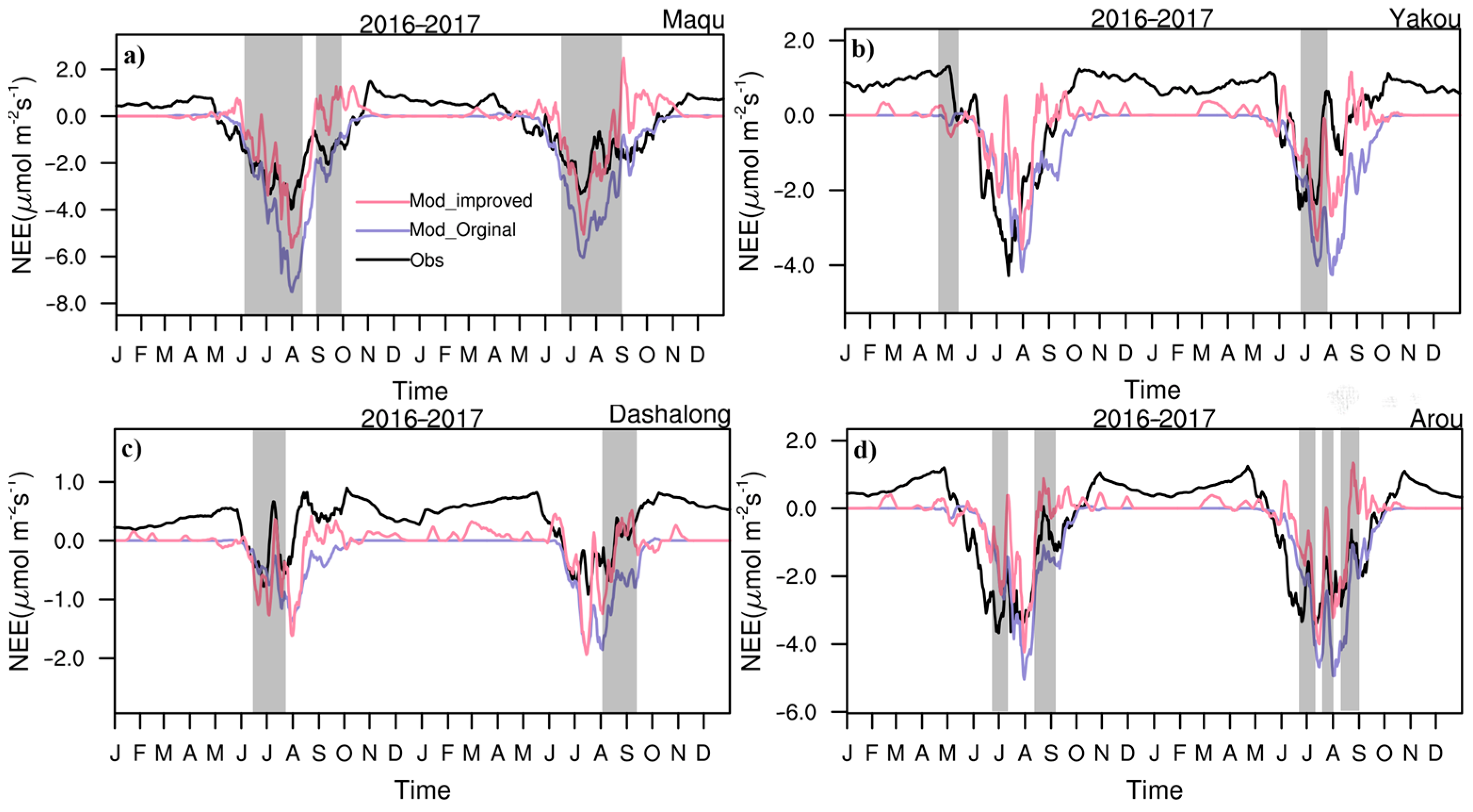
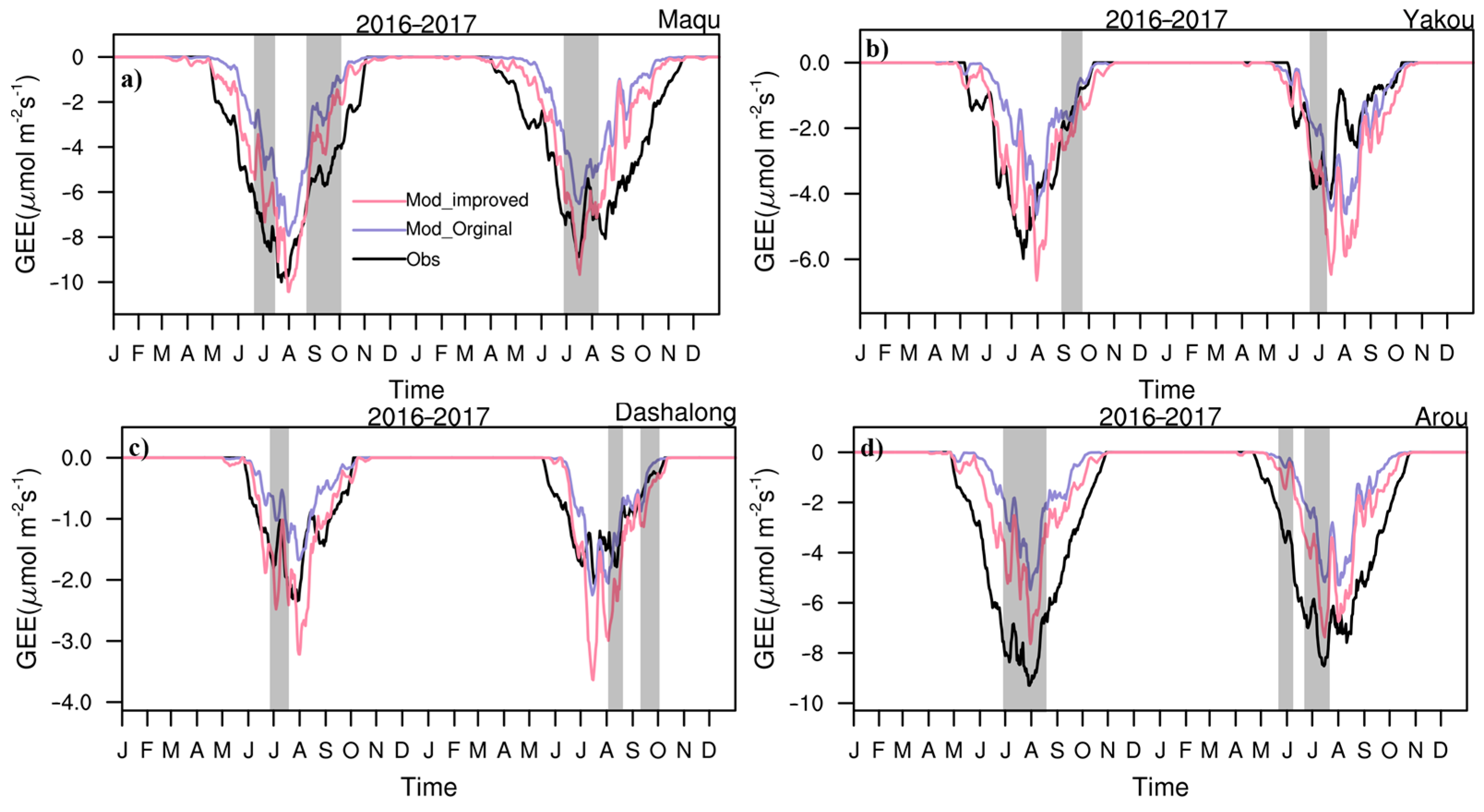
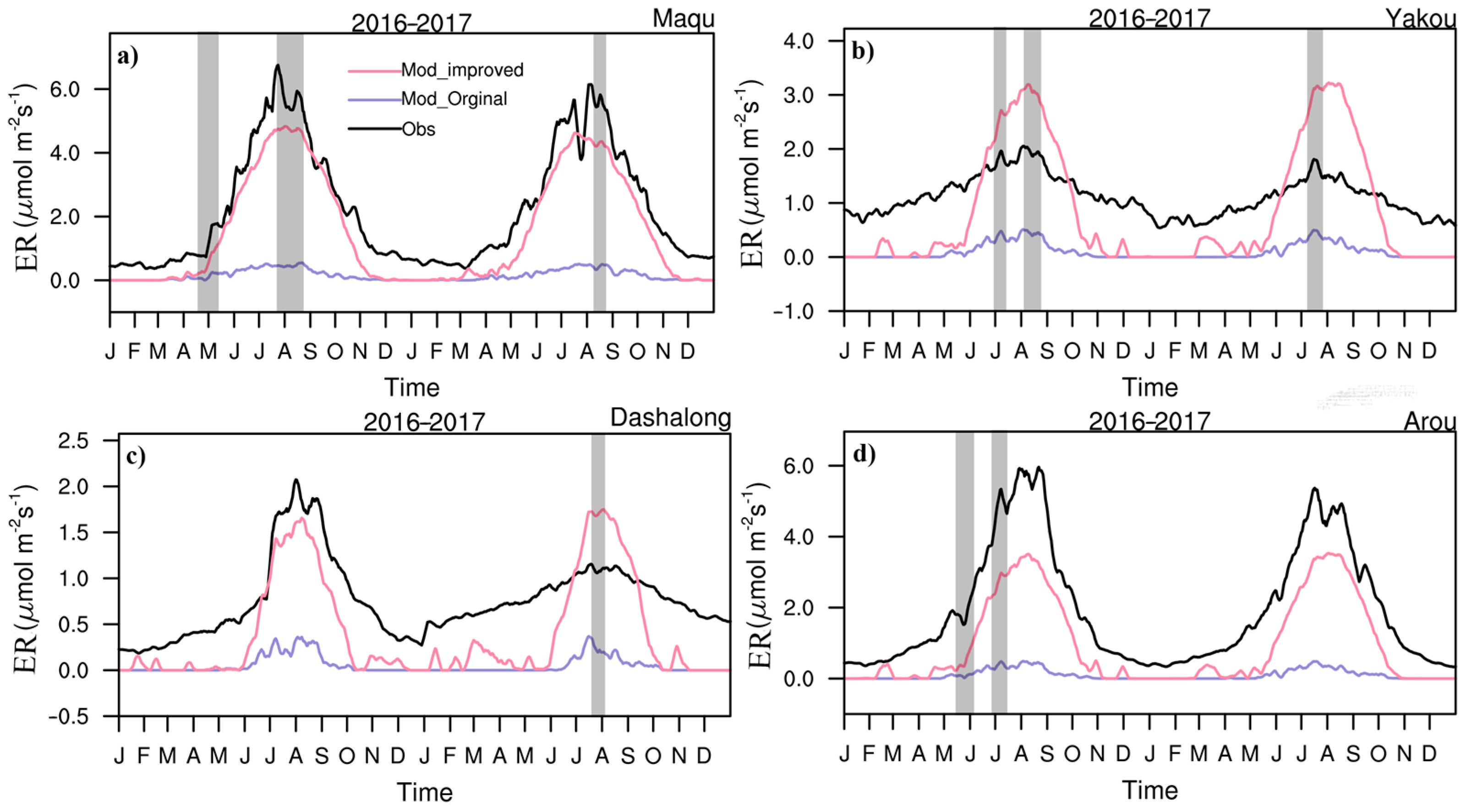
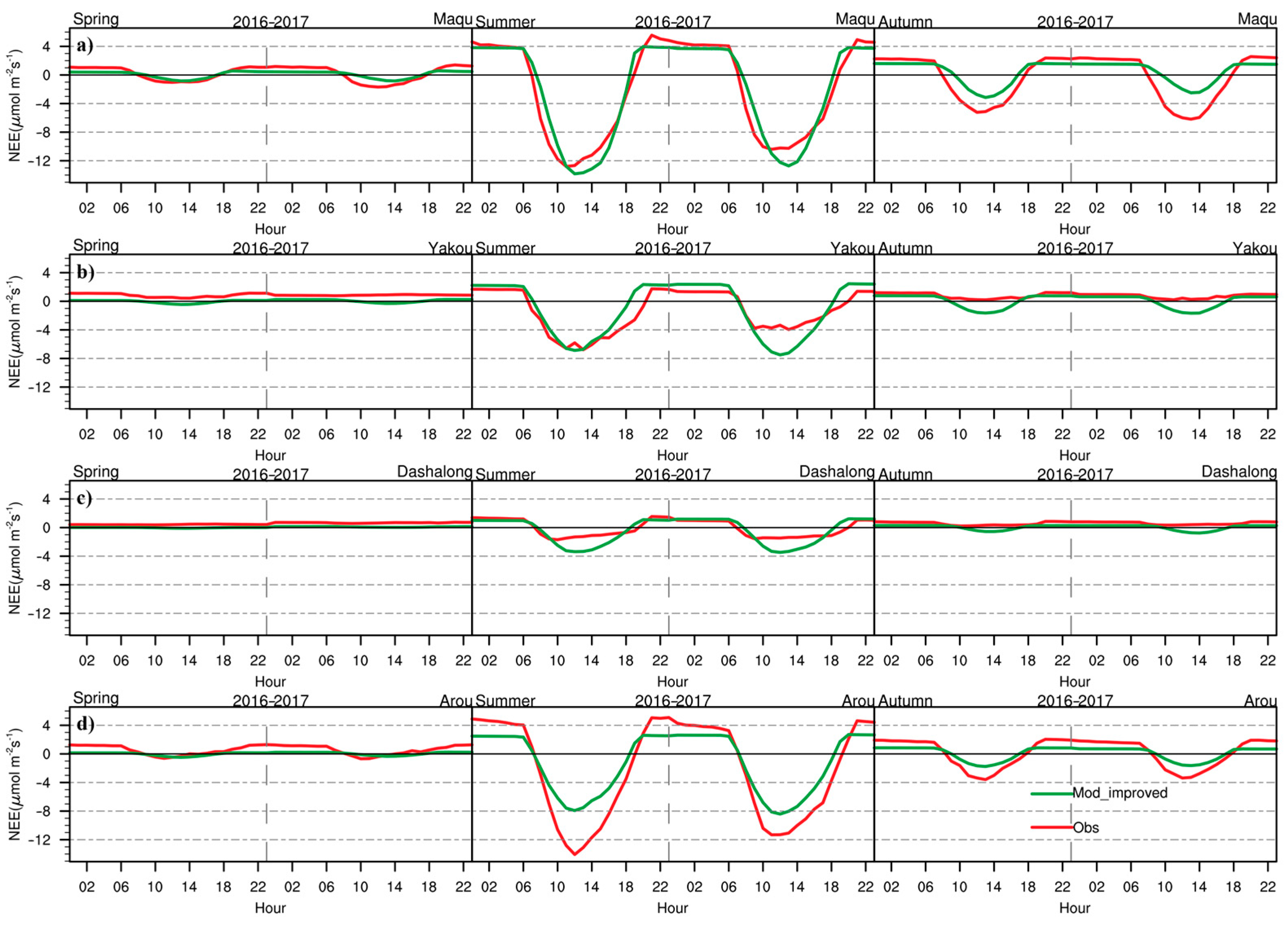
3.2. Daily Variations in CO₂ Fluxes during the Growing Season

Springtime observations revealed vigorous vegetation growth at Maqu and Arou, as reflected by the negative mid-day NEE values (Figure 7a,d), whereas ER dominated at Yakou (Figure 7b). Dashalong displayed no evident diurnal fluctuations, but an interannual increase in carbon emissions suggested heightened ER (Figure 7c). In summer, which marks the peak growing season, maximum NEE values of −13 μmol·m⁻²·s⁻¹ at Maqu were observed, with nighttime stabilization at approximately 4 μmol·m⁻²·s⁻¹ (Figure 7a). The NEE at Arou was consistent with that at Maqu. The observation results reached a maximum of −14 μmol·m⁻²·s⁻¹ at Arou, but the model slightly underestimated it (Figure 7d). Moreover, the carbon sink capacity at Yakou in summer was approximately half of that at Maqu (Figure 7b), and Dashalong showed relatively weaker carbon sink capacity than that of the other sites (Figure 7c). The NEE diurnal cycle in autumn was approximately 1 h later than that in summer. Yakou and Dashalong were completely transformed into carbon sources, indicating that the underlying surface played a key role in vegetation growth (Figure 7b,c). In the Maqu and Arou grasslands, although the fluctuations in NEE decreased, it remained negative during the day (Figure 7a,d). As the present study focused on changes in the growing season, diurnal changes in winter were not discussed.

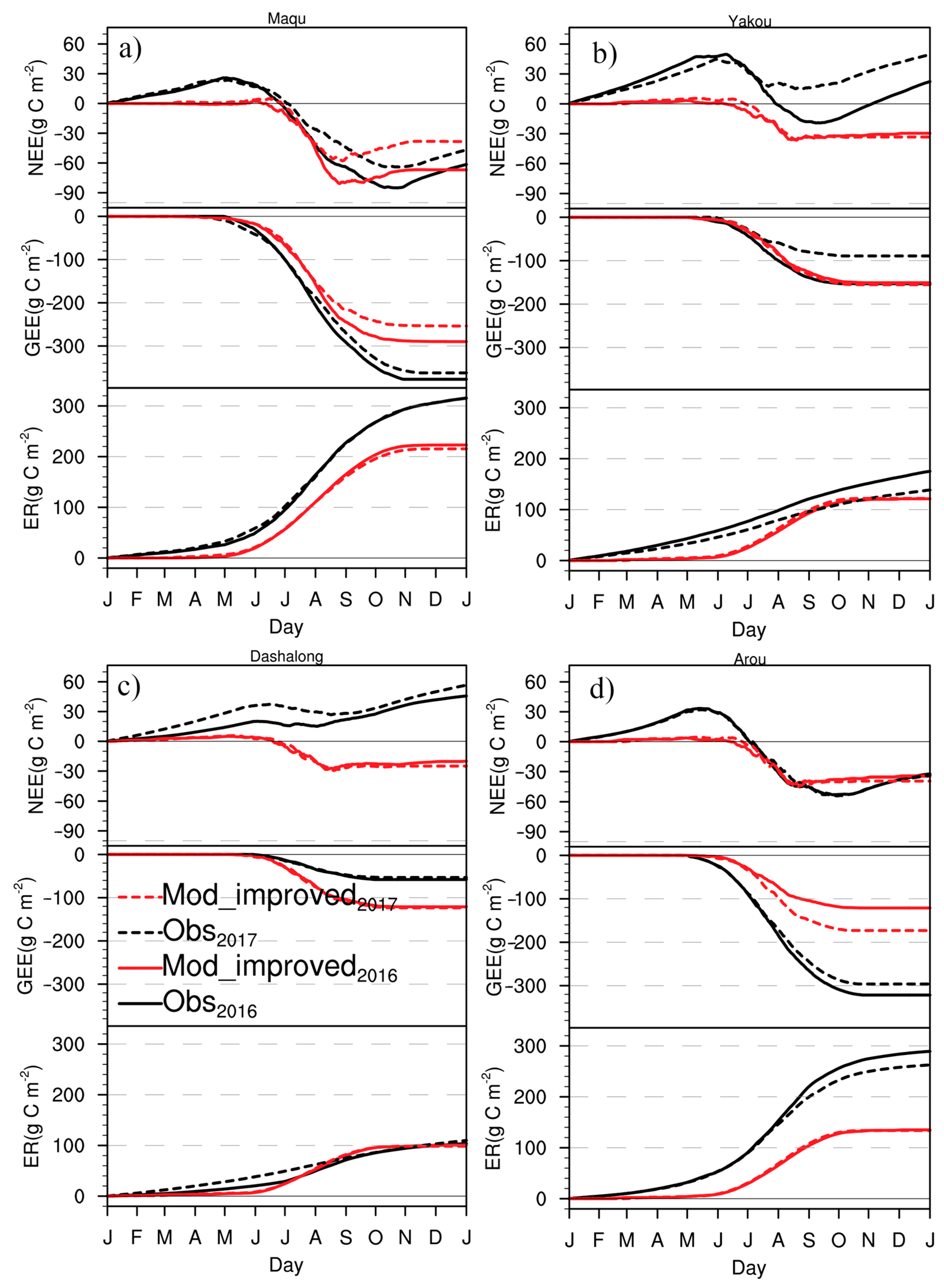
3.3. Cumulative CO₂ Fluxes

Figure 8 presents the cumulative fluxes of NEE, GEE, and ER over two consecutive years. Cumulative NEE increased from January to April or May owing to elevated ER caused by a steady temperature increase. Subsequently, the cumulative NEE started declining during the growing season at each site, and started increasing again after the growing season. When NEE was utilized for ecosystem source–sink analysis, different outcomes emerged across regions, with Maqu and Arou representing carbon sinks, and Yakou and Dashalong representing weak carbon sources. On comparing the cumulative carbon flux between the improved and original models based on previous results, we found an increase in cumulative carbon flux of 166.78, 197.8, 70.39, and 162.19% in 2016, and 186.92, 122.08, 68.64, and 195.59% in 2017, and ER improved by 63.55, 60.5, 85.3, and 41.52% in 2016, and 61.53, 78.86, 78.76, and 45.95% in 2017 at Maqu, Yakou, Dashalong, and Arou, respectively. Furthermore, the results of the improved model and observations were compared. The observational results suggest higher vegetation growth at Maqu and Arou than at Yakou and Dashalong. Cumulative GEE at the Maqu, Yakou, Dashalong, and Arou sites reached −376.932, −152.916, −57.942, and −321.633 gC·m⁻², respectively, in 2016 and −362.237, −89.126, −53.248, and −296.239 gC·m⁻², respectively, in 2017 (Figure 8a–d), while ER reached 315.517, 175.338, 103.722, and 327.017 gC·m⁻², respectively, in 2016, and 315.5 gC·m⁻², 138.531 gC·m⁻², 109.835 μmol·m⁻²·s⁻¹, and 262.647 μmol·m⁻²·s⁻¹, respectively, in 2017 (Figure 8a–d). Overall, the NEE, GEE, and ER were stronger in 2016 than in 2017 at all sites, indicating degraded carbon sink capacity that could be extremely detrimental to sustainable development.

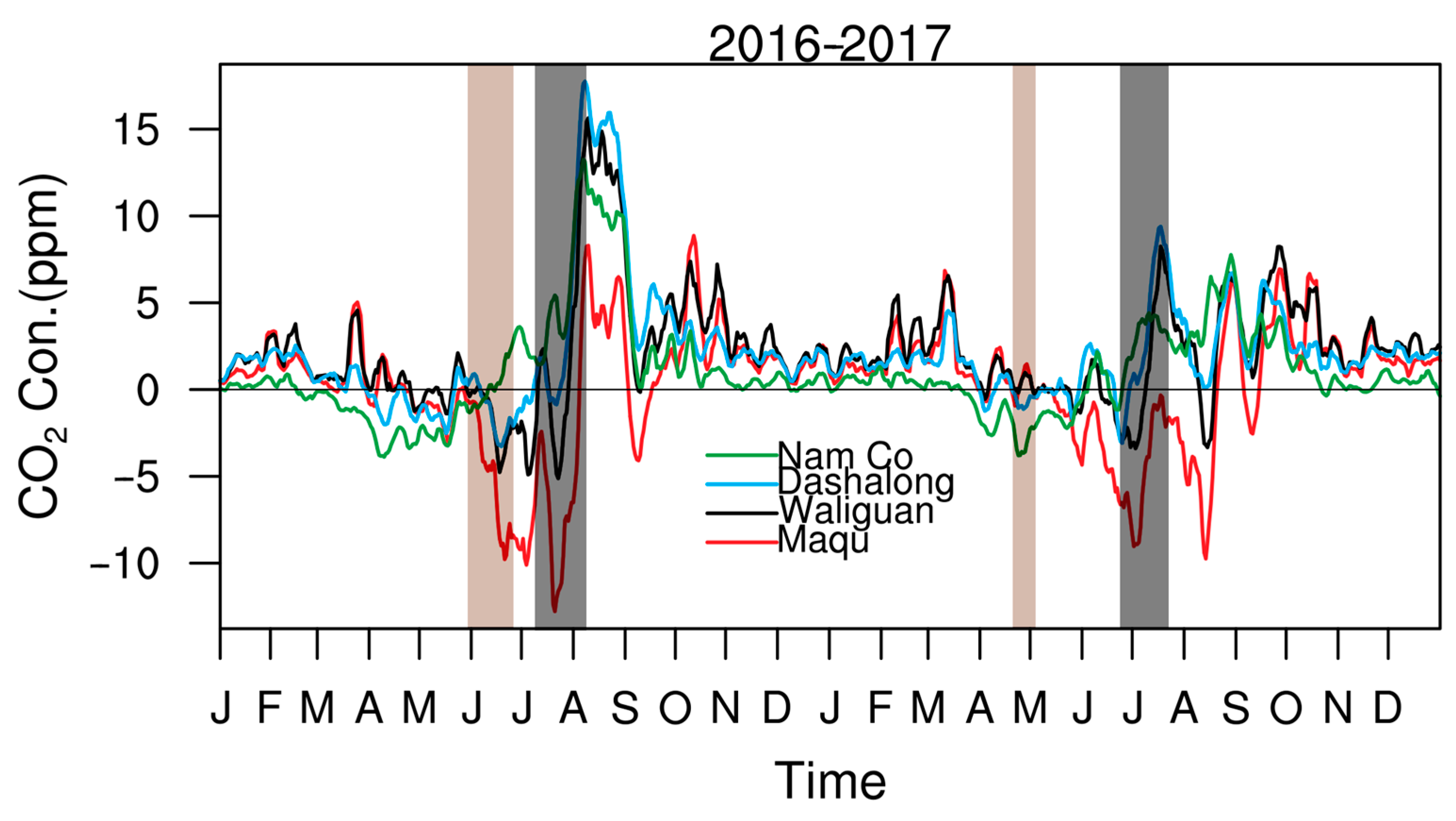
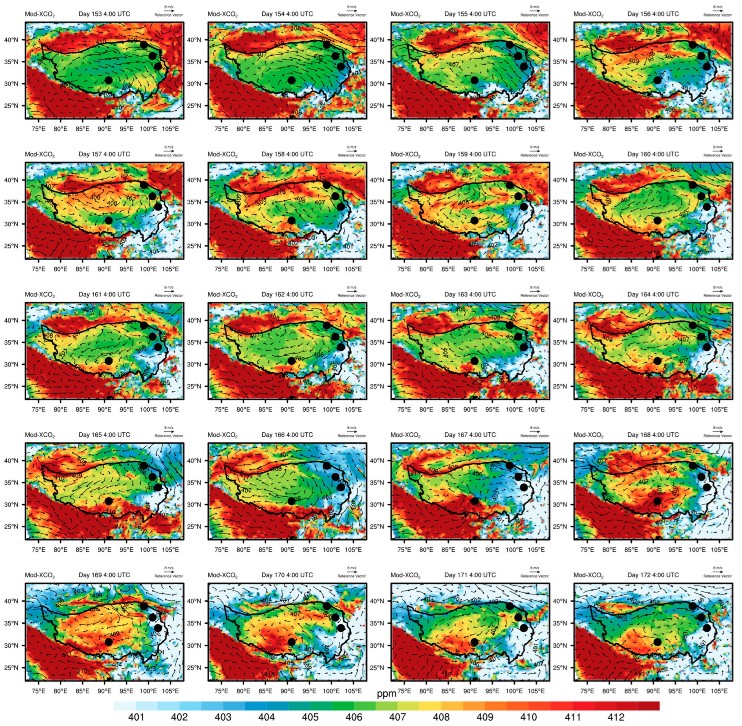
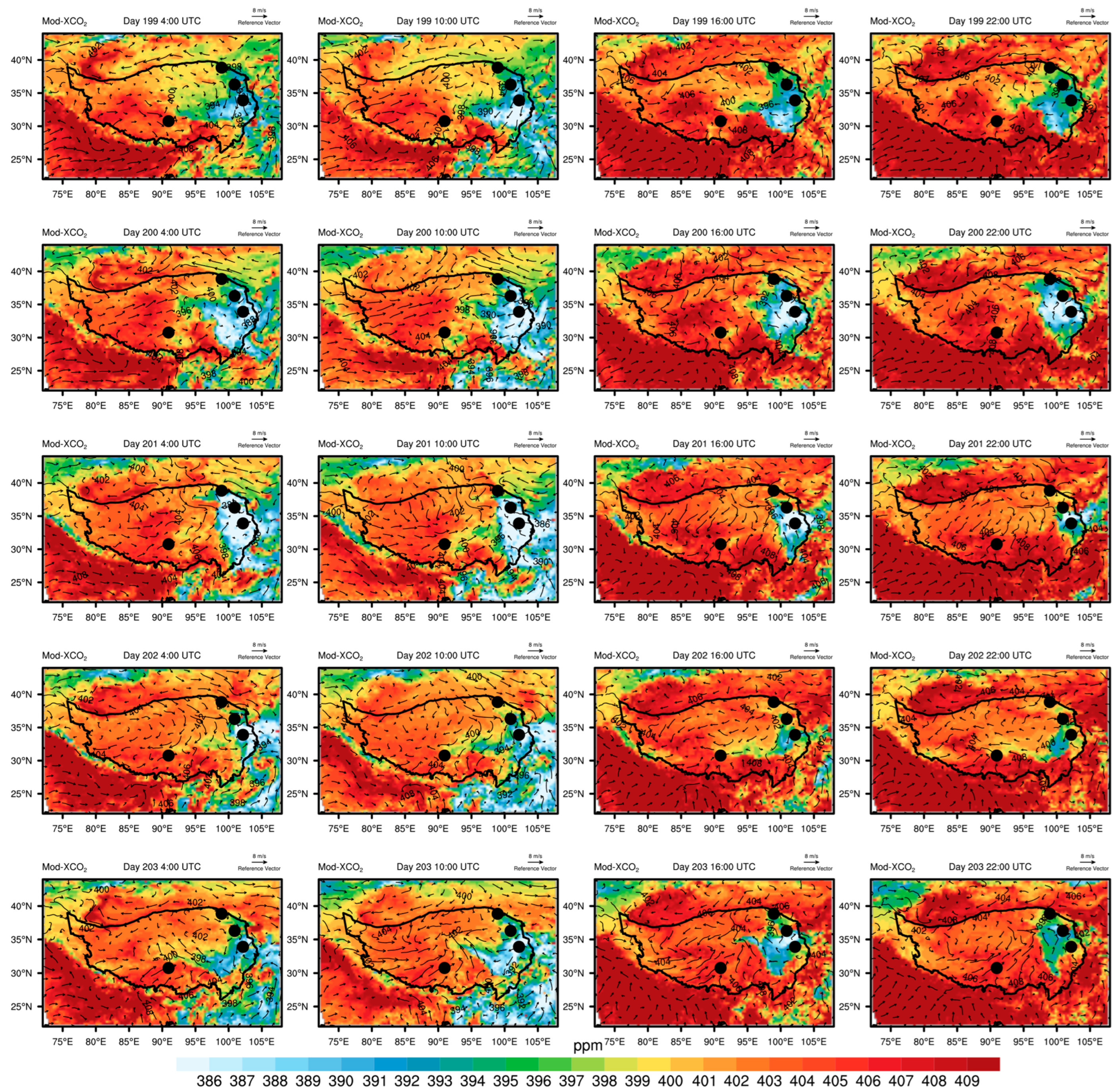
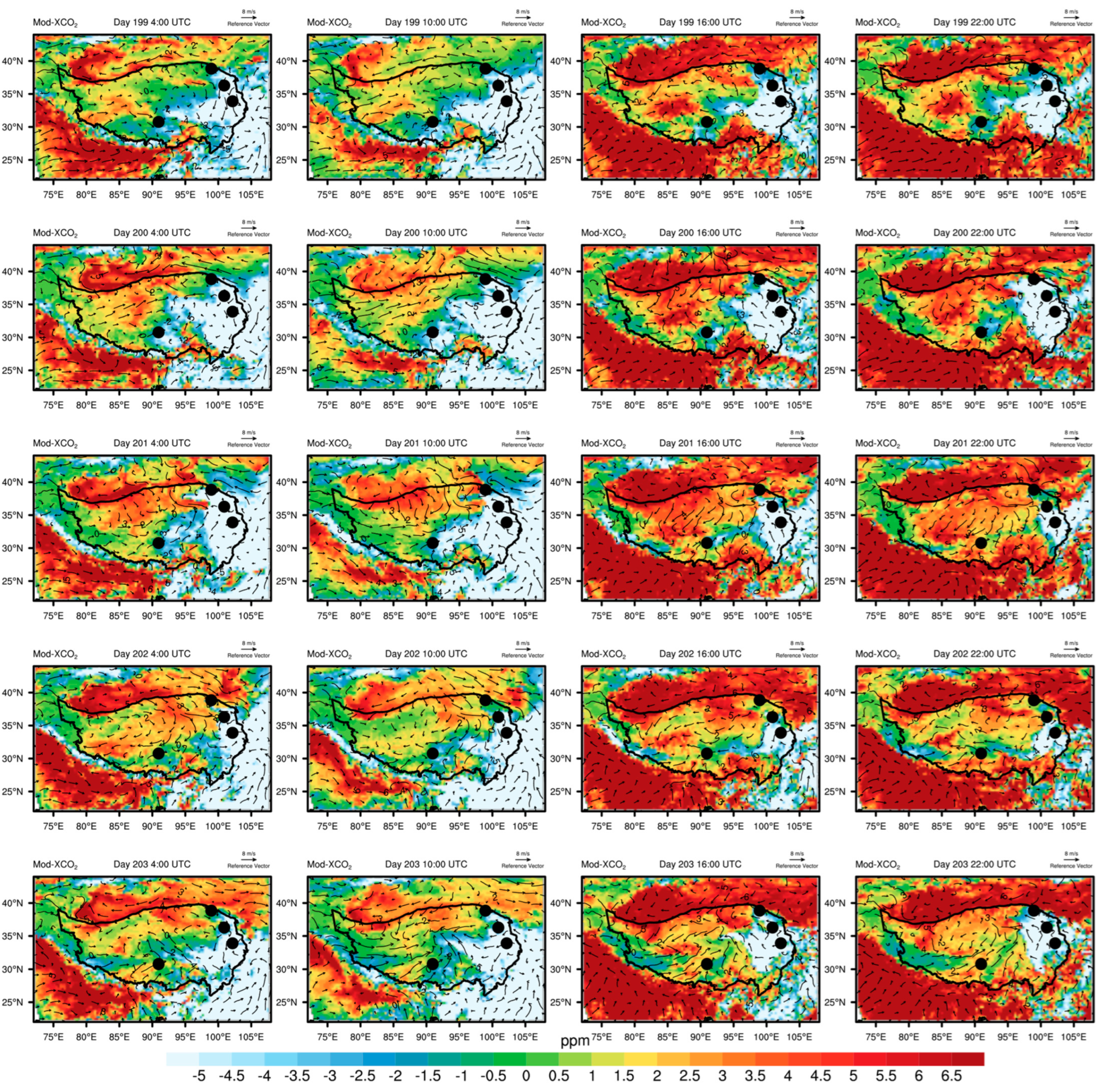
3.4. Irregular Variations in CO₂ Concentrations

Anomalies in CO₂ concentrations were calculated by deducting both background value and TP average variations from the local concentrations. Given the relatively minor fluctuations in CO₂ concentrations, four geographically distant sites were selected for the analysis. The 2-year average anomalies at Maqu, Waliguan, Dashalong, and Nam Co increased by 0.205, 2.196, 2.107, and 1.034 ppm, respectively, reflecting fast-rising CO₂ concentrations over the TP.

Local anomalies were observed when the curves from different stations showed contrasting trends. Conversely, global anomalies were observed when the trends were aligned. The analysis focused on CO₂ concentration anomalies in 2016, with local anomalies identified at 4:00 (UTC) daily from days 153 to 172 and global anomalies identified at 6 h intervals from 4:00 (UTC) on day 199 to 22:00 on day 203 (Figure 9). Local CO₂ concentration anomalies resulted primarily from horizontal transport. On day 153, the CO₂ concentrations at all four sites were closely aligned, with an average value of 407.230 ppm. Compared with the CO₂ concentration on day 153, the northwesterly winds dispersed the CO₂ at Maqu, resulting in a CO₂ concentration decrease of 1.795 ppm, and the deep southeasterly winds at the Nam Co site also decreased CO₂ concentration by 0.626 ppm (Figure 10). Subsequent shifts in wind direction influenced the CO₂ concentrations at Maqu and Nam Co from days 165 to 168, and on day 168, the CO₂ concentration at Maqu and Nam Co decreased by 6.744 and 2.308 ppm, respectively, compared with that on day 153 (Figure 10). As the wind intensified and expanded, the difference in CO₂ concentrations between the two sites reached 15 ppm. Despite this concentration being relatively lower than that of the background value, this change was consistent with the changes in NEE (Figure 2), demonstrating that prior uncoupled models assuming constant CO₂ concentrations could not capture such a phenomenon and highlighting the importance of CO₂ concentration simulation for precise NEE prediction.

Global anomalies often reflect a range of changes encompassing daily variations. The daily driving force of surface CO₂ concentrations usually comprises background values, biospheric CO₂, ocean absorption, and anthropogenic emissions. Anthropogenic emissions and biosphere absorption are often responsible for anomalies [68,69,70,71,72]. Starting from day 199, the eastern TP exhibited lower CO₂ concentrations compared with the relatively high concentrations in the central and western regions (Figure 11). When the easterly and westerly winds intersected in the eastern region, CO₂ concentrations remained relatively low. Over time, the CO₂ concentration anomaly increased significantly, driven by reduced biological absorption on the TP (Figure 12). A peak in CO₂ concentrations was observed on day 201. This amplitude change was also evident in the observations and simulations shown in Figure 2, illustrating that advection-induced changes in CO₂ concentrations and subsequent NEE variations are critical to dynamic changes. Figure 11 reveals persistently high CO₂ concentrations in regions with strong westerly winds, whereas southeasterly winds generated a band of low CO₂ concentrations over the TP, as exemplified on day 203. From the eastern part of the TP, surface CO₂ concentrations remained at 398 ppm at 4:00 UTC on day 199 and decreased to 388 ppm on day 200 due to the easterly winds. From day 201, the high-value area of approximately 404 ppm in the central and western regions shifted to the east with the westerly wind, reducing to 389 ppm in the eastern part on day 203. At the same time, high CO₂ concentrations (408 ppm) in the Midwest were observed from 16:00 to 22:00 UTC on days 199 to 200, owing to the convergence of easterly and westerly winds.

The northwestern region of the TP demonstrated relatively low biospheric CO₂ (Figure 12), a phenomenon closely linked to the regional vegetation status and water content. Diurnal fluctuations in vegetation photosynthesis were also observed in the 5-day cycle. Most biological absorption is related to vegetation, and CO₂ concentration fluctuations exhibited minimal sensitivity to wind direction and speed. However, because of the ecosystem diversity of the TP, biological uptake did not exhibit a consistent southeast-to-northwest decrease, but was indeed lower in the mid-northwest region (Figure 12). The eastern TP biospheric CO₂ concentrations reached 5 ppm for five consecutive days, while the western region exhibited a weak emission of 1 ppm, and the central region had a high emission area of 4 ppm due to drought. Simultaneously, the emissions in the Qaidam Basin consistently remained at 3–4.5 ppm unless strong southeasterly winds were incident. The overall biospheric CO₂ was between −5 and 5 ppm, with the main driver of this change being the inability of photosynthesis to occur at night.

4. Discussion

Although ER increased with the water stress adjustment, GEE and NEE also demonstrated changes in different magnitudes, indicating the interdependence of respiration and photosynthesis. The WRF-VPRM employed in this study using satellite data [34] presented a physical mechanism superior to that of traditional statistical models [35] and offered higher interpretability and output resolution [18]. Light use efficiency models often simulate correlations to 0.8 [73,74]. Further, NEE, GEE, ER, and CO₂ concentrations were analyzed, and the improvements in carbon flux were determined using statistical variables (bias, RMSE, r-value, and RSD), thus suggesting that considering water stress enhances the simulation accuracy of carbon flux on the TP, particularly for ER, which may be due to the semi-arid or sub-humid ecological conditions in the study area, leading to a sensitive carbon flux response to water stress. Water stress, a key factor in vegetation physiological processes, influences not only respiration and photosynthesis, but also root development, rhizome transport, and stomatal closure [75]. Hence, water stress should be considered when simulating CO₂ flux and CO₂ concentration changes on the TP. After incorporating water stress, the simulation experiments exhibited improved accuracy for respiration, expressing not only year-round changes, but also providing a more precise depiction of the intraday cycle. Moreover, respiratory feedback enhanced the simulation results of photosynthesis. Similar results were observed in other studies, where sensitivity of vegetation to water stress was proven by the high correlation between photosynthesis and respiration in semi-humid areas [18,39]. Simultaneously, due to the influence of EVI, the modeled NEE at the Nam Co site remained greater than 0 μmol·m⁻²·s⁻¹, indicating that the site was a carbon source, while the observed NEE showed that it was a carbon sink (Figure 13a). The EVIs observed by the satellite at Maqu and Nam Co differed six-fold, while the observed NEE differed by only a factor of two (Figure 13b). This discrepancy may stem from the insufficient spatial resolution of the simulation to accurately reflect the real situation owing to the complex underlying surface types on the TP, such as alpine grasslands, subalpine meadows, swamp grasslands, and alpine meadows. Hence, due to these complexities, further investigations are warranted.

The improved model distinctly demonstrated daily and annual changes in CO₂ fluxes under high spatiotemporal resolution simulations, providing valuable interpretations. Moreover, the fully coupled WRF-VPRM efficiently simulated the CO₂ concentration response to carbon fluxes, accurately showing that local variations in concentration are influenced by advection. Although the model simulation results are promising, the EVI-based model could only represent the combined effects of vegetation, water stress, and temperature stress. Hence, to better understand the dynamic changes in vegetation on the TP, further research is essential to enhance the parameterization schemes in the model. Further studies with more western site observations are required to validate the modeling results for the TP and optimize the simulation effects of different vegetation substrates and climate-sensitive areas in the model.

5. Conclusions

This study analyzed the application of WRF-VPRM for simulating carbon fluxes and CO₂ concentrations in the TP under water stress and examined the carbon flux characteristics through in situ observations. Relative to the original model, the bias demonstrated a transition from −0.086, 1.615, and −2.371 μmol·m⁻²·s⁻¹ to −0.008, 0.439, and −0.418 μmol·m⁻²·s⁻¹, while RMSE values shifted from 1.676, 2.364, and 2.493 μmol·m⁻²·s⁻¹ to 1.361, 2.039, and 0.754 μmol·m⁻²·s⁻¹, at the four sites over 2 years on the TP. The r and RSD of NEE changed from 0.559 to 0.563 and 0.46 to 0.444, GEE changed from 0.739 to 0.773 and 0.322 to 0.467, and ER changed from 0.787 to 0.915 and 0.672 to 1.272, respectively. Moreover, the CO₂ concentration of the improved model simulations better reproduced summer fluctuations across different regions over the TP and responded to NEE changes. Local CO₂ concentration anomalies were influenced by wind speed and direction, whereas the overall anomalies were controlled by biological uptake. Despite the varying degrees by which the simulation results were enhanced across different sites on the TP, the final outcomes were satisfactory. The study highlights the importance of highly interpretable light use models in capturing the responses of vegetation to changes in individual factors on the TP. Using satellite data for simulation, this study incorporated and expanded information for larger-scale simulations, providing more reliable estimates for studying the interaction between CO₂ concentration and flux over the TP, and has potential significance for advancing future research.

References

1. Piao, S.; Fang, J.; Ciais, P.; Peylin, P.; Huang, Y.; Sitch, S.; Wang, T. The carbon balance of terrestrial ecosystems in China. Nature 2009, 458, 1009–1013. [Google Scholar] [CrossRef] [PubMed]
2. Cox, P.M.; Betts, R.A.; Jones, C.D.; Spall, S.A.; Totterdell, I.J. Acceleration of global warming due to carbon-cycle feedbacks in a coupled climate model. Nature 2000, 408, 184–187. [Google Scholar] [CrossRef]
3. Friedlingstein, P.; Cox, P.; Betts, R.; Bopp, L.; von Bloh, W.; Brovkin, V.; Cadule, P.; Doney, S.; Eby, M.; Fung, I.; et al. Climate–Carbon Cycle Feedback Analysis: Results from the C4MIP Model Intercomparison. J. Clim. 2006, 19, 3337–3353. [Google Scholar] [CrossRef]
4. Pan, Y.; Birdsey, R.A.; Fang, J.; Houghton, R.; Kauppi, P.E.; Kurz, W.A.; Phillips, O.L.; Shvidenko, A.; Lewis, S.L.; Canadell, J.G. A large and persistent carbon sink in the world’s forests. Science 2011, 333, 988–993. [Google Scholar] [CrossRef] [PubMed]
5. Palmer, P.I.; Feng, L.; Baker, D.; Chevallier, F.; Bosch, H.; Somkuti, P. Net carbon emissions from African biosphere dominate pan-tropical atmospheric CO2 signal. Nat. Commun. 2019, 10, 3344. [Google Scholar] [CrossRef]
6. Baldocchi, D.; Falge, E.; Gu, L.H.; Olson, R.; Hollinger, D.; Running, S.; Anthoni, P.; Bernhofer, C.; Davis, K.; Evans, R.; et al. FLUXNET: A new tool to study the temporal and spatial variability of ecosystem-scale carbon dioxide, water vapor, and energy flux densities. Bull. Am. Meteorol. Soc. 2001, 82, 2415–2434. [Google Scholar] [CrossRef]
7. Su, Y.-g.; Wu, L.; Zhang, Y.-m. Characteristics of carbon flux in two biologically crusted soils in the Gurbantunggut Desert, Northwestern China. Catena 2012, 96, 41–48. [Google Scholar] [CrossRef]
8. Wang, H.; Li, X.; Xiao, J.; Ma, M.; Tan, J.; Wang, X.; Geng, L. Carbon fluxes across alpine, oasis, and desert ecosystems in northwestern China: The importance of water availability. Sci. Total Environ. 2019, 697, 133978. [Google Scholar] [CrossRef]
9. Running, S.W.; Nemani, R.R.; Heinsch, F.A.; Zhao, M.S.; Reeves, M.; Hashimoto, H. A continuous satellite-derived measure of global terrestrial primary production. Bioscience 2004, 54, 547–560. [Google Scholar] [CrossRef]
10. Keenan, T.F.; Gray, J.; Friedl, M.A.; Toomey, M.; Bohrer, G.; Hollinger, D.Y.; Munger, J.W.; O’Keefe, J.; Schmid, H.P.; Wing, I.S.; et al. Net carbon uptake has increased through warming-induced changes in temperate forest phenology. Nat. Clim. Chang. 2014, 4, 598–604. [Google Scholar] [CrossRef]
11. van der Velde, I.R.; van der Werf, G.R.; Houweling, S.; Maasakkers, J.D.; Borsdorff, T.; Landgraf, J.; Tol, P.; van Kempen, T.A.; van Hees, R.; Hoogeveen, R.; et al. Vast CO2 release from Australian fires in 2019-2020 constrained by satellite. Nature 2021, 597, 366–369. [Google Scholar] [CrossRef] [PubMed]
12. Ye, X.X.; Lauvaux, T.; Kort, E.A.; Oda, T.; Feng, S.; Lin, J.C.; Yang, E.G.; Wu, D. Constraining Fossil Fuel CO2 Emissions From Urban Area Using OCO-2 Observations of Total Column CO2. J. Geophys. Res.-Atmos. 2020, 125, e2019JD030528. [Google Scholar] [CrossRef]
13. Labzovskii, L.D.; Jeong, S.J.; Parazoo, N.C. Working towards confident spaceborne monitoring of carbon emissions from cities using Orbiting Carbon Observatory-2. Remote Sens. Environ. 2019, 233, 111359. [Google Scholar] [CrossRef]
14. Fu, P.; Xie, Y.H.; Moore, C.E.; Myint, S.W.; Bernacchi, C.J. A Comparative Analysis of Anthropogenic CO2 Emissions at City Level Using OCO-2 Observations: A Global Perspective. Earths Future 2019, 7, 1058–1070. [Google Scholar] [CrossRef]
15. Ciais, P.; Reichstein, M.; Viovy, N.; Granier, A.; Ogee, J.; Allard, V.; Aubinet, M.; Buchmann, N.; Bernhofer, C.; Carrara, A.; et al. Europe-wide reduction in primary productivity caused by the heat and drought in 2003. Nature 2005, 437, 529–533. [Google Scholar] [CrossRef]
16. Beer, C.; Reichstein, M.; Tomelleri, E.; Ciais, P.; Jung, M.; Carvalhais, N.; Rodenbeck, C.; Arain, M.A.; Baldocchi, D.; Bonan, G.B.; et al. Terrestrial Gross Carbon Dioxide Uptake: Global Distribution and Covariation with Climate. Science 2010, 329, 834–838. [Google Scholar] [CrossRef]
17. Cho, S.; Kang, M.; Ichii, K.; Kim, J.; Lim, J.-H.; Chun, J.-H.; Park, C.-W.; Kim, H.S.; Choi, S.-W.; Lee, S.-H.; et al. Evaluation of forest carbon uptake in South Korea using the national flux tower network, remote sensing, and data-driven technology. Agric. For. Meteorol. 2021, 311, 108653. [Google Scholar] [CrossRef]
18. Li, X.; Hu, X.M.; Cai, C.; Jia, Q.; Zhang, Y.; Liu, J.; Xue, M.; Xu, J.; Wen, R.; Crowell, S.M.R. Terrestrial CO2 Fluxes, Concentrations, Sources and Budget in Northeast China: Observational and Modeling Studies. J. Geophys. Res. Atmos. 2020, 125, e2019JD031686. [Google Scholar] [CrossRef]
19. Dong, X.Y.; Yue, M.; Jiang, Y.J.; Hu, X.M.; Ma, Q.L.; Pu, J.J.; Zhou, G.Q. Analysis of CO2 spatio-temporal variations in China using a weather-biosphere online coupled model. Atmos. Chem. Phys. 2021, 21, 7217–7233. [Google Scholar] [CrossRef]
20. Wei, D.; Qi, Y.; Ma, Y.; Wang, X.; Ma, W.; Gao, T.; Huang, L.; Zhao, H.; Zhang, J.; Wang, X. Plant uptake of CO2 outpaces losses from permafrost and plant respiration on the Tibetan Plateau. Proc. Natl. Acad. Sci. USA 2021, 118, e2015283118. [Google Scholar] [CrossRef]
21. Liu, H.Y.; Mi, Z.R.; Lin, L.; Wang, Y.H.; Zhang, Z.H.; Zhang, F.W.; Wang, H.; Liu, L.L.; Zhu, B.A.; Cao, G.M.; et al. Shifting plant species composition in response to climate change stabilizes grassland primary production. Proc. Natl. Acad. Sci. USA 2018, 115, 4051–4056. [Google Scholar] [CrossRef] [PubMed]
22. Ding, J.Z.; Chen, L.Y.; Ji, C.J.; Hugelius, G.; Li, Y.N.; Liu, L.; Qin, S.Q.; Zhang, B.B.; Yang, G.B.; Li, F.; et al. Decadal soil carbon accumulation across Tibetan permafrost regions. Nat. Geosci. 2017, 10, 420–424. [Google Scholar] [CrossRef]
23. Schuur, E.A.G.; Abbott, B.; Permafrost Carbon, N. High risk of permafrost thaw. Nature 2011, 480, 32–33. [Google Scholar] [CrossRef] [PubMed]
24. Schneider von Deimling, T.; Meinshausen, M.; Levermann, A.; Huber, V.; Frieler, K.; Lawrence, D.M.; Brovkin, V. Estimating the near-surface permafrost-carbon feedback on global warming. Biogeosciences 2012, 9, 649–665. [Google Scholar] [CrossRef]
25. Piao, S.L.; Wang, X.H.; Park, T.; Chen, C.; Lian, X.; He, Y.; Bjerke, J.W.; Chen, A.P.; Ciais, P.; Tommervik, H.; et al. Characteristics, drivers and feedbacks of global greening. Nat. Rev. Earth Environ. 2020, 1, 14–27. [Google Scholar] [CrossRef]
26. Kroel-Dulay, G.; Mojzes, A.; Szitar, K.; Bahn, M.; Batary, P.; Beier, C.; Bilton, M.; De Boeck, H.J.; Dukes, J.S.; Estiarte, M.; et al. Field experiments underestimate aboveground biomass response to drought. Nat. Ecol. Evol. 2022, 6, 540–545. [Google Scholar] [CrossRef]
27. De Cannière, S.; Herbst, M.; Vereecken, H.; Defourny, P.; Jonard, F. Constraining water limitation of photosynthesis in a crop growth model with sun-induced chlorophyll fluorescence. Remote Sens. Environ. 2021, 267, 112722. [Google Scholar] [CrossRef]
28. Huete, A.R.; Liu, H.Q.; Batchily, K.; vanLeeuwen, W. A comparison of vegetation indices global set of TM images for EOS-MODIS. Remote Sens. Environ. 1997, 59, 440–451. [Google Scholar] [CrossRef]
29. Xiao, X.; Hollinger, D.; Aber, J.; Goltz, M.; Davidson, E.A.; Zhang, Q.; Moore, B. Satellite-based modeling of gross primary production in an evergreen needleleaf forest. Remote Sens. Environ. 2004, 89, 519–534. [Google Scholar] [CrossRef]
30. Churkina, G.; Schimel, D.; Braswell, B.H.; Xiao, X.M. Spatial analysis of growing season length control over net ecosystem exchange. Glob. Chang. Biol. 2005, 11, 1777–1787. [Google Scholar] [CrossRef]
31. Jenkins, J.P.; Richardson, A.D.; Braswell, B.H.; Ollinger, S.V.; Hollinger, D.Y.; Smith, M.L. Refining light-use efficiency calculations for a deciduous forest canopy using simultaneous tower-based carbon flux and radiometric measurements. Agric. For. Meteorol. 2007, 143, 64–79. [Google Scholar] [CrossRef]
32. Sims, D.; Rahman, A.; Cordova, V.; Elmasri, B.; Baldocchi, D.; Bolstad, P.; Flanagan, L.; Goldstein, A.; Hollinger, D.; Misson, L. A new model of gross primary productivity for North American ecosystems based solely on the enhanced vegetation index and land surface temperature from MODIS. Remote Sens. Environ. 2008, 112, 1633–1646. [Google Scholar] [CrossRef]
33. Houborg, R.; Soegaard, H.; Boegh, E. Combining vegetation index and model inversion methods for the extraction of key vegetation biophysical parameters using Terra and Aqua MODIS reflectance data. Remote Sens. Environ. 2007, 106, 39–58. [Google Scholar] [CrossRef]
34. Ahmadov, R.; Gerbig, C.; Kretschmer, R.; Koerner, S.; Neininger, B.; Dolman, A.J.; Sarrat, C. Mesoscale covariance of transport and CO2 fluxes: Evidence from observations and simulations using the WRF-VPRM coupled atmosphere-biosphere model. J. Geophys. Res.-Atmos. 2007, 112, D2210. [Google Scholar] [CrossRef]
35. Mahadevan, P.; Wofsy, S.C.; Matross, D.M.; Xiao, X.; Dunn, A.L.; Lin, J.C.; Gerbig, C.; Munger, J.W.; Chow, V.Y.; Gottlieb, E.W. A satellite-based biosphere parameterization for net ecosystem CO2 exchange: Vegetation Photosynthesis and Respiration Model (VPRM). Glob. Biogeochem. Cycles 2008, 22, GB2005. [Google Scholar] [CrossRef]
36. Vázquez-Lule, A.; Vargas, R. Proximal remote sensing and gross primary productivity in a temperate salt marsh. Agric. For. Meteorol. 2023, 341, 109639. [Google Scholar] [CrossRef]
37. Gupta, S.; Burman, P.K.D.; Tiwari, Y.K.; Dumka, U.C.; Kumari, N.; Srivastava, A.; Raghubanshi, A.S. Understanding carbon sequestration trends using model and satellite data under different ecosystems in India. Sci. Total Environ. 2023, 897, 166381. [Google Scholar] [CrossRef] [PubMed]
38. Fan, F.F.; Xiao, C.W.; Feng, Z.M.; Yang, Y.Z. Impact of human and climate factors on vegetation changes in mainland southeast asia and yunnan province of China. J. Clean. Prod. 2023, 415, 137690. [Google Scholar] [CrossRef]
39. Hu, X.M.; Gourdji, S.M.; Davis, K.J.; Wang, Q.; Zhang, Y.; Xue, M.; Feng, S.; Moore, B.; Crowell, S.M.R. Implementation of Improved Parameterization of Terrestrial Flux in WRF-VPRM Improves the Simulation of Nighttime CO2 Peaks and a Daytime CO2 Band Ahead of a Cold Front. J. Geophys. Res. Atmos. 2021, 126, e2020JD034362. [Google Scholar] [CrossRef]
40. Hu, X.M.; Crowell, S.; Wang, Q.; Zhang, Y.; Davis, K.J.; Xue, M.; Xiao, X.; Moore, B.; Wu, X.; Choi, Y.; et al. Dynamical Downscaling of CO2 in 2016 Over the Contiguous United States Using WRF-VPRM, a Weather-Biosphere-Online-Coupled Model. J. Adv. Model. Earth Syst. 2020, 12, e2019MS001875. [Google Scholar] [CrossRef]
41. Raoult, N.; Charbit, S.; Dumas, C.; Maignan, F.; Ottlé, C.; Bastrikov, V. Improving modelled albedo over the Greenland ice sheet through parameter optimisation and MODIS snow albedo retrievals. Cryosphere 2023, 17, 2705–2724. [Google Scholar] [CrossRef]
42. Bacour, C.; MacBean, N.; Chevallier, F.; Léonard, S.; Koffi, E.N.; Peylin, P. Assimilation of multiple datasets results in large differences in regional- to global-scale NEE and GPP budgets simulated by a terrestrial biospheremodel. Biogeosciences 2023, 20, 1089–1111. [Google Scholar] [CrossRef]
43. Yang, S.Y.; Zhao, B.X.; Yang, D.W.; Wang, T.H.; Yang, Y.T.; Ma, T.; Santisirisomboon, J. Future changes in water resources, floods and droughts under the joint impact of climate and land-use changes in the Chao Phraya basin, Thailand. J. Hydrol. 2023, 620, 129454. [Google Scholar] [CrossRef]
44. Song, X.; Zheng, B.F.; Hu, F.Q.; Xu, L.L.; Wu, H.Q.; Liu, Z.; Wan, W. Divergent Responses of NPP to Climate Factors among Forest Types at Interannual and Inter-Monthly Scales: An Empirical Study on Four Typical Forest Types in Subtropical China. Forests 2023, 14, 1474. [Google Scholar] [CrossRef]
45. Kretschmer, R.; Gerbig, C.; Karstens, U.; Koch, F.T. Error characterization of CO2 vertical mixing in the atmospheric transport model WRF-VPRM. Atmos. Chem. Phys. 2012, 12, 2441–2458. [Google Scholar] [CrossRef]
46. Pillai, D.; Gerbig, C.; Ahmadov, R.; Rodenbeck, C.; Kretschmer, R.; Koch, T.; Thompson, R.; Neininger, B.; Lavric, J.V. High-resolution simulations of atmospheric CO2 over complex terrain—Representing the Ochsenkopf mountain tall tower. Atmos. Chem. Phys. 2011, 11, 7445–7464. [Google Scholar] [CrossRef]
47. Raich, J.W.; Rastetter, E.B.; Melillo, J.M.; Kicklighter, D.W.; Steudler, P.A.; Peterson, B.J.; Grace, A.L.; Moore, B.; Vorosmarty, C.J. Potential Net Primary Productivity In South-America—Application Of A Global-Model. Ecol. Appl. 1991, 1, 399–429. [Google Scholar] [CrossRef]
48. Lee, Y.-H.; Park, S.-U. Evaluation of a modified soil–plant–atmosphere model for CO2 flux and latent heat flux in open canopies. Agric. For. Meteorol. 2007, 143, 230–241. [Google Scholar] [CrossRef]
49. Joetzjer, E.; Delire, C.; Douville, H.; Ciais, P.; Decharme, B.; Carrer, D.; Verbeeck, H.; DeWeirdt, M.; Bonal, D. Improving the ISBA(CC) land surface model simulation of water and carbon fluxes and stocks over the Amazon forest. Geosci. Model Dev. 2015, 8, 1709–1727. [Google Scholar] [CrossRef]
50. Zhang, T.; Zhang, Y.; Xu, M.; Zhu, J.; Chen, N.; Jiang, Y.; Huang, K.; Zu, J.; Liu, Y.; Yu, G. Water availability is more important than temperature in driving the carbon fluxes of an alpine meadow on the Tibetan Plateau. Agric. For. Meteorol. 2018, 256–257, 22–31. [Google Scholar] [CrossRef]
51. Cao, G.; Tang, Y.; Mo, W.; Wang, Y.; Li, Y.; Zhao, X. Grazing intensity alters soil respiration in an alpine meadow on the Tibetan plateau. Soil Biol. Biochem. 2004, 36, 237–243. [Google Scholar] [CrossRef]
52. Kato, T.; Tang, Y.; Gu, S.; Hirota, M.; Du, M.; Li, Y.; Zhao, X. Temperature and biomass influences on interannual changes in CO2. exchange in an alpine meadow on the Qinghai-Tibetan Plateau. Glob. Chang. Biol. 2006, 12, 1285–1298. [Google Scholar] [CrossRef]
53. Zhao, L.; Li, Y.; Xu, S.; Zhou, H.; Gu, S.; Yu, G.; Zhao, X. Diurnal, seasonal and annual variation in net ecosystem CO2 exchange of an alpine shrubland on Qinghai-Tibetan plateau. Glob. Chang. Biol. 2006, 12, 1940–1953. [Google Scholar] [CrossRef]
54. Zhuang, Q.; He, J.; Lu, Y.; Ji, L.; Xiao, J.; Luo, T. Carbon dynamics of terrestrial ecosystems on the Tibetan Plateau during the 20th century: An analysis with a process-based biogeochemical model. Glob. Ecol. Biogeogr. 2010, 119, 649–662. [Google Scholar] [CrossRef]
55. Chen, J.; Luo, Y.; Xia, J.; Shi, Z.; Jiang, L.; Niu, S.; Zhou, X.; Cao, J. Differential responses of ecosystem respiration components to experimental warming in a meadow grassland on the Tibetan Plateau. Agric. For. Meteorol. 2016, 220, 21–29. [Google Scholar] [CrossRef]
56. Li, H.; Zhang, F.; Li, Y.; Wang, J.; Zhang, L.; Zhao, L.; Cao, G.; Zhao, X.; Du, M. Seasonal and inter-annual variations in CO2 fluxes over 10 years in an alpine shrubland on the Qinghai-Tibetan Plateau, China. Agric. For. Meteorol. 2016, 228–229, 95–103. [Google Scholar] [CrossRef]
57. Li, X.; Cheng, G.D.; Liu, S.M.; Xiao, Q.; Ma, M.G.; Jin, R.; Che, T.; Liu, Q.H.; Wang, W.Z.; Qi, Y.; et al. Heihe Watershed Allied Telemetry Experimental Research (HiWATER): Scientific Objectives and Experimental Design. Bull. Am. Meteorol. Soc. 2013, 94, 1145–1160. [Google Scholar] [CrossRef]
58. Liu, S.M.; Xu, Z.W.; Song, L.S.; Zhao, Q.Y.; Ge, Y.; Xu, T.R.; Ma, Y.F.; Zhu, Z.L.; Jia, Z.Z.; Zhang, F. Upscaling evapotranspiration measurements from multi-site to the satellite pixel scale over heterogeneous land surfaces. Agric. For. Meteorol. 2016, 230, 97–113. [Google Scholar] [CrossRef]
59. Liu, S.M.; Xu, Z.W.; Wang, W.Z.; Jia, Z.Z.; Zhu, M.J.; Bai, J.; Wang, J.M. A comparison of eddy-covariance and large aperture scintillometer measurements with respect to the energy balance closure problem. Hydrol. Earth Syst. Sci. 2011, 15, 1291–1306. [Google Scholar] [CrossRef]
60. Shang, L.; Zhang, Y.; Lyu, S.; Wang, S. Seasonal and Inter-Annual Variations in Carbon Dioxide Exchange over an Alpine Grassland in the Eastern Qinghai-Tibetan Plateau. PLoS ONE 2016, 11, e0166837. [Google Scholar] [CrossRef]
61. Nieberding, F.; Wille, C.; Fratini, G.; Asmussen, M.O.; Wang, Y.Y.; Ma, Y.M.; Sachs, T. A long-term (2005-2019) eddy covariance data set of CO2 and H2O fluxes from the Tibetan alpine steppe. Earth Syst. Sci. Data 2020, 12, 2505–2524. [Google Scholar] [CrossRef]
62. Wu, F.Q.; Guo, S.M.; Huang, W.B.; Han, Y.C.; Wang, Z.B.; Wang, G.P.; Li, X.F.; Lei, Y.P.; Yang, B.F.; Xiong, S.W.; et al. Adaptation of cotton production to climate change by sowing date optimization and precision resource management. Ind. Crops Prod. 2023, 203, 117167. [Google Scholar] [CrossRef]
63. Omazic, B.; Prtenjak, M.T.; Bubola, M.; Mestric, J.; Karoglan, M.; Prsa, I. Application of statistical models in the detection of grapevine phenology changes. Agric. For. Meteorol. 2023, 341, 109682. [Google Scholar] [CrossRef]
64. Huete, A.; Didan, K.; Miura, T.; Rodriguez, E.P.; Gao, X.; Ferreira, L.G. Overview of the radiometric and biophysical performance of the MODIS vegetation indices. Remote Sens. Environ. 2002, 83, 195–213. [Google Scholar] [CrossRef]
65. Pillai, D.; Gerbig, C.; Marshall, J.; Ahmadov, R.; Kretschmer, R.; Koch, T.; Karstens, U. High resolution modeling of CO2 over Europe: Implications for representation errors of satellite retrievals. Atmos. Chem. Phys. 2010, 10, 83–94. [Google Scholar] [CrossRef]
66. Kanamitsu, M.; Ebisuzaki, W.; Woollen, J.; Yang, S.K.; Hnilo, J.J.; Fiorino, M.; Potter, G.L. NCEP-DOE AMIP-II reanalysis (R-2). Bull. Am. Meteorol. Soc. 2002, 83, 1631–1643. [Google Scholar] [CrossRef]
67. Meng Xianhong, L.I.Z. Meteorological Observation Data at Maqu Grassland Site from 2017 to 2020; National Tibetan Plateau Data Center: 2022. Available online: https://data.tpdc.ac.cn/en/data/3966b5db-9a4f-44e0-afac-4a1eedc2cfce/ (accessed on 9 October 2022).
68. Weir, B.; Crisp, D.; O’Dell, C.W.; Basu, S.; Chatterjee, A.; Kolassa, J.; Oda, T.; Pawson, S.; Poulter, B.; Zhang, Z.; et al. Regional impacts of COVID-19 on carbon dioxide detected worldwide from space. Sci. Adv. 2021, 7, eabf9415. [Google Scholar] [CrossRef]
69. Sheng, M.Y.; Lei, L.P.; Zeng, Z.C.; Rao, W.Q.; Zhang, S.Q. Detecting the Responses of CO2 Column Abundances to Anthropogenic Emissions from Satellite Observations of GOSAT and OCO-2. Remote Sens. 2021, 13, 3524. [Google Scholar] [CrossRef]
70. Miglietta, F.; Raschi, A.; Resti, R.; Badiani, M. Growth and onto-morphogenesis of soybean (Glycine max Merril) in an open, naturally CO2-enriched environment. Plant Cell Environ. 1993, 16, 909–918. [Google Scholar] [CrossRef]
71. Li, K.F. An Intraseasonal Variability in CO2 Over the Arctic Induced by the Madden-Julian Oscillation. Geophys. Res. Lett. 2018, 45, 1630–1638. [Google Scholar] [CrossRef]
72. Hakkarainen, J.; Ialongo, I.; Maksyutov, S.; Crisp, D. Analysis of Four Years of Global XCO2 Anomalies as Seen by Orbiting Carbon Observatory-2. Remote Sens. 2019, 11, 850. [Google Scholar] [CrossRef]
73. Xie, J.; Yin, G.; Ma, D.; Chen, R.; Zhao, W.; Xie, Q.; Wang, C.; Lin, S.; Yuan, W. Climatic limitations on grassland photosynthesis over the Tibetan Plateau shifted from temperature to water. Sci. Total Environ. 2023, 906, 167663. [Google Scholar] [CrossRef] [PubMed]
74. Wang, S.; Huang, K.; Yan, H.; Yan, H.; Zhou, L.; Wang, H.; Zhang, J.; Yan, J.; Zhao, L.; Wang, Y.; et al. Improving the light use efficiency model for simulating terrestrial vegetation gross primary production by the inclusion of diffuse radiation across ecosystems in China. Ecol. Complex. 2015, 23, 1–13. [Google Scholar] [CrossRef]
75. Farooq, M.; Wahid, A.; Kobayashi, N.; Fujita, D.; Basra, S.M.A. Plant drought stress: Effects, mechanisms and management. Agron. Sustain. Dev. 2009, 29, 185–212. [Google Scholar] [CrossRef]
Figure 1. Distribution of research sites on the Tibetan Plateau according to the (a) enhanced vegetation index and (b) land surface water index. Panoramic views of the sites: (c) Maqu, (d) Dashalong, (e) Arou, (f) Yakou, (g) Nam Co, and (h) Mt. Waliguan. Image (c) was sourced from Meng [67], while images (df) were taken from Liu [58]. Image (h) was acquired from the China Meteorological News Agency.
Remotesensing 15 05474 g001
Figure 2. Seasonal variations in net ecosystem exchange (NEE) from 2016 to 2017. The shaded areas indicate that the model captured the observed fluctuations, reflecting the changes in CO2 concentration.
Remotesensing 15 05474 g002
Figure 3. Seasonal variations in gross ecosystem exchange (GEE) during 2016–2017. The shaded areas indicate that the model captured the observed fluctuations, reflecting the changes in CO2 concentration.
Remotesensing 15 05474 g003
Figure 4. Seasonal variations in ecosystem respiration (ER) during 2016–2017. The shaded areas indicate that the model captured the observed fluctuations, reflecting the changes in CO2 concentration.
Remotesensing 15 05474 g004
Figure 5. Diurnal variations in net ecosystem exchange (NEE) from days 180 to 185 of 2016 (left) and 2017 (right) at the peak of the growing season at (a,b) Maqu, (c,d) Yakou, (e,f) Dashalong, and (g,h) Arou. Horizontal lines indicate that photosynthesis and interactions are in balance at night.
Remotesensing 15 05474 g005
Figure 6. Daily changes in CO2 concentrations in 2016 and 2017. CO2 concentration data from various sources are presented: site observations (red), original model (blue), and improved model (green).
Remotesensing 15 05474 g006
Figure 7. Average diurnal variations in net ecosystem exchange (NEE) during the growing season. Left panels: the beginning of the growing season in spring; middle panels: peak of the growing season in summer; and right panels: end of the growing season in autumn.
Remotesensing 15 05474 g007
Figure 8. Cumulative NEE, GEE, and ER. NEE, net ecosystem exchange; GEE, gross ecosystem exchange; and ER, ecosystem respiration.
Remotesensing 15 05474 g008
Figure 9. Irregular changes in CO2 concentration for two consecutive years. Brown and gray shading indicate local and overall anomalies, respectively.
Remotesensing 15 05474 g009
Figure 10. CO2 concentration changes simulated by the improved WRF-VPRM considering the wind on days 153–172 at 4:00 (UTC) each day in 2016. The four black dots are the observation sites mentioned in Figure 9 with 8 m·s−1 wind speeds.
Remotesensing 15 05474 g010
Figure 11. Overall anomalous changes in the CO2 concentration simulated by the improved WRF-VPRM from 4:00 (UTC) every 6 h on days 199–203 in 2016 at the four observation sites with 8 m·s−1 wind speeds.
Remotesensing 15 05474 g011
Figure 12. Biospheric CO2 concentrations varied in the simulation by the improved WRF-VPRM from 4:00 (UTC) every 6 h on days 199–203 of 2016 at the four observation sites with 8 m·s−1 wind speeds.
Remotesensing 15 05474 g012
Figure 13. (a). Daily changes in net ecosystem exchange (NEE) during 2016–2017 at Nam Co. (b). Net ecosystem exchange (NEE) observations at sites with daily enhanced vegetation index (EVI) variation.
Remotesensing 15 05474 g013