Abstract
Earth system models (ESMs) are important tools for assessing the historical characteristics and predicting the future characteristics of precipitation, yet the quantitative understanding of how these land–atmospheric coupling models perform in simulating precipitation characteristics remains limited. This study conducts a comprehensive evaluation of precipitation changes simulated by 43 ESMs in CMIP5 and 32 ESMs in CMIP6 in Arid Central Asia (ALL) and its two sub-regions for 1959–2005 with reference to Climate Research Unit (CRU) data, and predicts precipitation changes for 2054–2100. Our analyses suggest the following: (a) no single model consistently outperformed the others in all aspects of simulated precipitation variability (annual averages, long-term trends, and climatological monthly patterns); (b) the CMIP5 and CMIP6 model simulations tended to overestimate average annual precipitation for most of the ALL region, especially in the Xinjiang Uygur Autonomous Region of China (XJ); (c) most model simulations projected a stronger increasing trend in average annual precipitation; (d) although all the model simulations reasonably captured the climatological monthly precipitation, there was an underestimation; (e) compared to CMIP5, most CMIP6 model simulations exhibited an enhanced capacity to simulate precipitation across all aspects, although discrepancies persisted in individual sub-regions; (f) it was confirmed that the multi-model ensemble mean (MME) provides a more accurate representation of the three aspects of precipitation compared to the majority of single-model simulations. Lastly, the values of precipitation predicted by the more efficient models across the ALL region and its sub-regions under the different scenarios showed an increasing trend in most seasons. Notably, the strongest increasing trend in precipitation was seen under the high-emission scenarios.
1. Introduction
Global warming has caused alterations in the spatial and temporal patterns of precipitation, exerting profound impacts on water resources [1], ecosystems [2,3], and socio-economics [4]. As a vital element within the terrestrial hydrological cycle, precipitation serves a dual purpose by depositing fresh water on the planet and indirectly regulating the flux exchanges between the land and the atmosphere [5]. Many studies have evaluated the impact of historical precipitation evolution on global environmental changes using ground-based observations, satellite-based data, and reanalysis products at global and regional scales [6,7,8]. However, the utility of these datasets in global precipitation analyses is limited [9], which is primarily due to the short duration of precipitation records [10].
Global circulation models (GCMs) serve as potent tools for simulating the interactions among the atmosphere, oceans, land surface, and ice [11,12,13,14]. They are pivotal for comprehending and anticipating the intricate alterations and fluctuations in precipitation triggered by climate change on both global and regional scales. Climate models participating in the fifth phase of the Coupled Model Intercomparison Project (CMIP5) are used to examine the response of the climate system to both anthropogenic and natural external forcings [15]. To verify the accuracy of these model simulations, numerous efforts have been made to evaluate the performance of CMIP5 in simulating precipitation at global and regional scales [16,17]. For instance, Liu et al. [16] evaluated 34 GCMs from CMIP5 over global land between 1901 and 2005 and showed variability in their precipitation simulation capabilities both spatially and temporally. These studies offer a rich repository of insights and serve as valuable references for model developers and users, contributing to a better understanding of the strengths, weaknesses, and areas of improvement in precipitation simulation across different CMIP5 model simulations. Representative concentration pathways (RCPs) are a set of comprehensive concentration and emission scenarios, used as input parameters for climate change prediction models under the influence of human activities in the 21st century in CMIP5 [18]. They outline the variations in greenhouse gas, reactive gas, and aerosol emissions, as well as atmospheric composition concentrations, when changes occur in aspects like population, socio-economics, science and technology, energy consumption, and land use in the future.
However, CMIP5 model simulations are inevitably subject to uncertainties stemming from model structure, parameterization, hypotheses, calibration processes, etc. [19,20,21,22,23]. These uncertainties, when coupled with different climate forcings, can lead to widely different precipitation outputs from models. Previous studies have reported long-standing biases in the total precipitation generated from those global models in terms of magnitude, variability, and changing direction [16,24,25,26], which pose substantial uncertainties on the associated hydrological or climate change analyses and consequent scientific findings. The Coupled Model Intercomparison Project Phase 6 (CMIP6) provides a new generation of global climate model data [27]. Compared to the previous generation, CMIP5, CMIP6 has two major distinct features: firstly, the processes considered in the models are more refined and complex, with many models achieving the bidirectional coupling of atmosphere and chemistry; secondly, there is a significant increase in spatial resolution for both atmospheric and oceanic models [28], thereby enhancing the ability of climate models in historical simulation and future estimation, satisfying more complex Earth system science research, and strengthening the understanding and recognition of climate change’s driving mechanisms [28]. Additionally, the inclusion of shared socioeconomic pathways (SSPs) under the CMIP6 model and representative concentration pathway (RCP) scenarios under the CMIP5 model, which account for the effects of socioeconomic development, provides a more accurate representation of the potential outcomes of climate change. Indeed, some studies have reported overall improvement in the capability of CMIP6 models to globally simulate precipitation [29,30,31]. However, suboptimal performance has been reported in areas of complex terrain and extreme climate zones, such as semi-arid and arid regions [32,33]. Previous studies have individually assessed the capabilities of these two generations of models in simulating precipitation [34,35]. For example, Ta et al. [36] assessed 37 GCMs from CMIP5 over Central Asia between 1986 and 2005 and showed variability in their precipitation simulation capabilities both spatially and temporally. Guo et al. [37] assessed 30 GCMs from CMIP6 over Central Asia between 1951 and 2014 in the aspects of annual mean, intra-annual variability, and long-term trends. Zhang et al. [38] assessed 42 climate models within CMIP6 and found that these models could reproduce the overall spatial patterns of daily precipitation in the Xinjiang (XJ) region. However, they noted that the bias in precipitation amounts exhibited variation across different seasons. To our knowledge, it remains unresolved whether the CMIP6 models demonstrate superior performance compared to the CMIP5 models in simulating precipitation changes across various dimensions, including annual mean, intra-annual variability, inter-annual variability, and long-term trends. This knowledge gap greatly hampers the selection of the most appropriate datasets of CMIP model simulations for specific applications in Central Asia for end-users.
Additionally, prior studies primarily concentrated on examining the historical evolution of precipitation within specific regions [39,40], with limited exploration of future precipitation trends under different scenarios from CMIP model simulations. This dearth of research has greatly hindered the development of mitigation strategies and measures for local responses to climate change.
This study employs Arid Central Asia as an example (Figure 1). The Arid Central Asia region is the largest arid area in the northern hemisphere’s temperate and warm temperate zones, encompassing the five Central Asian countries (Kazakhstan, Tajikistan, Kyrgyzstan, Uzbekistan, and Turkmenistan) and the arid region of Northwestern China. Situated deep in the continental interior, it’s hard for marine air currents to reach this region. Additionally, the Tien Shan mountains and Pamir Plateau block the moisture from the Pacific and Indian Oceans, rendering Central Asia minimally affected by marine influences. Under the dominance of westerly circulation, the moisture primarily comes from the Atlantic and Arctic Oceans. The region’s annual average precipitation is less than 150 mm, with a highly uneven spatial distribution, and mountainous areas receive more precipitation than basins and plains. As the world’s largest non-zonal arid region, Arid Central Asia is exceptionally vulnerable to climate change [41], exacerbating its already severe water-related challenges [42]. Previous research has shown that Central Asia has experienced an average rate of temperature increase of 0.18 °C decade−1 over the past century, which is comparable to the warming rate of the Qinghai–Tibet Plateau and significantly higher than that of other Northern Hemisphere regions [43]. Alongside warming, total precipitation is projected to increase, with a decreased likelihood of snowfall [44]. In this study, Arid Central Asia is spatially segmented into two distinct parts: the five Central Asian countries (CA) and the Xinjiang Uygur Autonomous Region of China (XJ). This segmentation is aligned with administrative boundaries, as Xinjiang is a region within China, whereas the other specified regions are independent countries. Additionally, this division resonates with the pronounced disparities in dryness and humidity changes observed between the two regions [45].
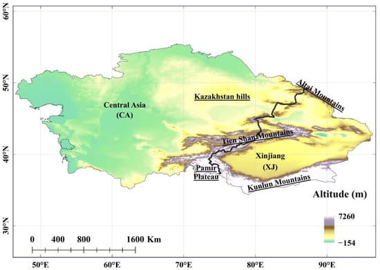
Figure 1.
Topographic map of Arid Central Asia. The black line in the figure indicates the boundary between the two sub-regions.
This study has a dual purpose: (i) to discern whether the CMIP6 models surpass the CMIP5 models in their ability to accurately simulate precipitation changes across various dimensions, including annual means, intra-annual variability, inter-annual variability, and long-term trend perspectives, and (ii) to ascertain the impending shifts in precipitation patterns within Arid Central Asia under various future RCPs and SSPs predicted by the CMIP5 and CMIP6 model simulations. The findings of this study can provide valuable scientific references for end-users seeking to apply CMIP5 and CMIP6 precipitation simulations tailored to the unique requirements of Arid Central Asia.
2. Materials and Methods
2.1. Data
The gridded precipitation dataset used in this study as the observational precipitation product was derived from the latest Climate Research Unit (CRU) (https://crudata.uea.ac.uk/cru/data/hrg/cru_ts_4.04/ (accessed on 5 January 2023)) based on more than 4000 meteorological stations, such as the monthly climate bulletins (CLIMAT), the Global Historical Climatology Network (GHCN-v2), and ad hoc station collections [46] (Figure S1). This product spans the period from 1901 to 2019, with a spatial resolution of 25 km and a monthly temporal resolution. The improvements in the latest version of the CRU (CRU TS v4.04 is used in this study) were achieved through the Angular Distance Weighting (ADW) technique and included the use of extra meteorological stations. As the CRU data predominantly depend on information sourced from surface meteorological observation stations, the uneven distribution of these stations may result in inadequate observation data in certain regions [47,48]. Furthermore, there are variations in observation instruments and measurement methodologies among different meteorological sites [49,50], and these differences may lead to uncertainties in the observations.
Despite these uncertainties, validation against in situ measurements from the Northern Hemisphere indicates that the CRU exhibits a relative accuracy of 88%, and it has found widespread application in climate research [51,52], hydrological processes [53], and other scientific applications. Considering the limited availability of meteorological stations in Arid Central Asia before 1955 and the cutoff year of historical model simulations being 2005, the precipitation data of the CRU from 1959 to 2005 were taken in this study to ensure the accuracy of observational data and temporal consistency with the model simulations.
With the development of satellite remote sensing technology, more and more satellite-retrieval precipitation products are beginning to be widely used [54,55]. Since satellites retrieve precipitation data by observing cloud top temperature, cloud backscatter, and other information [56], coupled with certain errors in the algorithms, there are many instances of missed precipitation and false precipitation in satellite-retrieved precipitation products [57]. Currently, there are several kinds of precipitation inversion algorithms for different sensors on satellites [58], and there has been a gradual shift to fusing precipitation products from multiple sensors to obtain more accurate precipitation information [59]. These high-quality satellite precipitation inversion data play a vital role in different fields such as climate [60], hydrology [61], and agriculture [62]. Multi-Source Weighted-Ensemble Precipitation (MSWEP) (https://www.gloh2o.org/mswep/ (accessed on 20 March 2023)) is a comprehensive precipitation dataset crafted to furnish high-resolution precipitation data at a global scale [63]. Its data sources include ground-based observations, satellite remote sensing inversion, and reanalysis data. MSWEP data offer a high spatial resolution of 0.1°, and its temporal coverage spans from 1979 to the present day.
The usability of MSWEP data for long time series analyses is limited by temporal continuity constraints. By establishing a correlation between the CRU data and the MSWEP data, our analyses reveal a highly significant relationship between the CRU data and the MSWEP data in Arid Central Asia, with R2 values as high as 0.92 (Figure S2). This result allows us to consider CRU data as a substitute for satellite data in our study and to use CRU data as a benchmark to assess the ability of the CMIP model to simulate precipitation in Arid Central Asia.
2.2. Climate Model Simulations
Monthly outputs of historical precipitation (1959–2005) and future (2006–2100) periods were obtained from 43 CMIP5 model simulations (https://esgf-node.llnl.gov/search/cmip5/ (accessed on 10 April 2023)) and 32 CMIP6 model simulations (https://esgf-node.llnl.gov/projects/cmip6/ (accessed on 21 April 2023)) (Tables S1 and S2). In the CMIP5 future simulations, we used three RCPs with different forcing levels (RCP 2.6, RCP 4.5, and RCP 8.5) [64], and in the CMIP6 experiments, we used the SSP1-2.6, SSP2-4.5, and SSP5-8.5 scenarios to simulate future trends. To reduce variability across models caused by the ensemble means of numerous of realizations, only the first runs from each model were considered (r1i1p1 and r1i1p1f1, respectively) across all CMIP5 and CMIP6 models. For simulation and evaluation purposes, a first-order conservative method [65] was used in this study to resample the outputs of all models. They were resampled to the same size with a 0.5° spatial resolution with reference to the observed data.
2.3. Evaluation Metric Methods
In this study, six frequently employed statistical metrics were utilized to assess the simulated precipitation: (i) Taylor diagram and Taylor scale score (TSS); (ii) Pearson’s correlation coefficient (r); (iii) root mean square error (RMSE); (iv) standard deviation (STD); (v) absolute bias (AE); and (vi) comprehensive rating index (CRI). Evaluation analysis was performed for the whole year, spring (March–May, MAM), summer (June–August, JJA), autumn (September–November, SON), and winter (December–February, DJF), and individual months. The details of these methods are described below:
The Taylor diagram, as introduced by Taylor in 2001 [66], serves as a tool to assess the capacity of model simulations to reproduce the spatial distribution of annual precipitation patterns, considering r, RMSE, and STD. In these metrics, a lower RMSE, a higher r value, and an STD approximating 1 collectively signify close alignment of the spatial pattern of annual precipitation, as simulated by the models, with the observed data.
For the quantitative evaluation of each model’s capacity to replicate spatial patterns of annual precipitation (for the entire year and different seasons), we employed the TSS from Taylor [66]. The TSS is computed using the following formula:
where represents the spatial correlation coefficient between the model and observational data, while and denote the STD of the observed data and model simulations, respectively. The TSS values span from 0 to 1, and when they approach 1, it signifies a more accurate simulation of the spatial pattern of annual precipitation.
Pearson’s correlation coefficient, r, describes the consistency of variability between the model simulations and observational data [67], with the value of r ranging from −1 to 1. In this context, the stronger the correlation between the model simulations and the observed data, the closer the absolute value of r is to 1. r is computed as follows:
where and denote the ESMs and the mean of ESMs, and and denote the observational data and mean observed value, respectively.
RMSE is a widely used metric for quantifying the overall discrepancy between simulations and observations [68,69,70]. RMSE is inherently non-negative, and a smaller RMSE signifies superior model performance. The formula for calculating RMSE is as follows:
where denotes the ESMs, and denotes the observational data.
STD compares the simulated and observed precipitation variabilities and is calculated as follows:
where and represent the observed data (model simulation) and the average of the observed data (model simulation average), respectively. AE measures the ability of the model simulations to capture climatological precipitation with observation data. AE is calculated as follows:
where and represent the model simulations and observed data, respectively.
Finally, the CRI ranks the overall performance of model simulations [71,72]. Here, the CRI values are calculated using the TSS, bias, r, and RMSE obtained from each model simulation. Subsequently, the average of the CRI values derived from various models within each institution is computed to evaluate the collective modeling performance of different institutions in both the CMIP5 and CMIP6 model simulations. The CRI is calculated using the following formula:
where represents the count of indices utilized for assessing model performance, while denotes the multi-model ensemble mean (MME) and signifies the total number of model institutions. The top-performing model is assigned a rank value of 1. Consequently, a CRI value closer to 1 indicates a higher level of performance for the model institution.
3. Results
3.1. Mean Annual Precipitation and Long-Term Trend from Observational Data
Figure 2 illustrates the spatial distribution of annual average precipitation and its long-term trend across the ALL region from 1959 to 2005. The central area, encompassing the Pamir Plateau, Tien Shan Mountains, eastern Kazakhstan hills, and northern Kazakhstan, exhibits high mean annual precipitation exceeding 300 mm (Figure 2a). The central south of the Pamir Plateau receives the highest precipitation, with a mean annual precipitation of up to 800 mm. In contrast, other regions within the CA region experience a mean annual precipitation below 200 mm. During MAM, SON, and DJF, precipitation is primarily concentrated in the CA region, whereas during JJA, except for the Pamir Plateau and the Karakoram Mountains, precipitation is more uniformly distributed across the other regions.
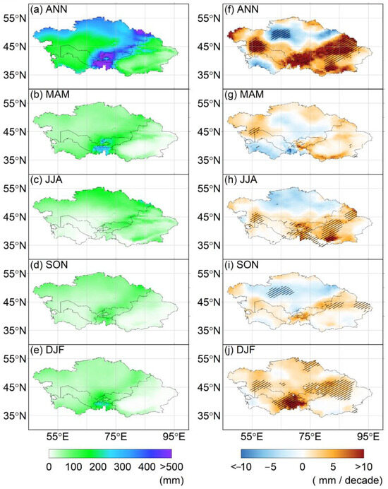
Figure 2.
Spatial patterns of the statistics of precipitation in the ALL area from the CRU data between 1959 and 2005. Left column: annual mean precipitation (mm); right column: trends of precipitation (mm/decade). First row: for the whole year (ANN); second row: for MAM; third row: for JJA; fourth row: for SON; fifth row: for DJF. The diagonal slashes in the regions signify statistical significance at the 95% confidence level (p < 0.05), determined using a two-tailed Student’s t-test.
A long-term trend analysis of precipitation from 1959 to 2005 reveals distinct seasonal variations. Considering the entire year, approximately 74% of the ALL region displays an upward trend in precipitation. Notably, significant trends are observed in the southern and western areas of the CA region, as well as extensive areas in the XJ region. Conversely, a declining trend is noticeable in the southwestern and northern regions of the CA region, with significant decreases in certain northwestern regions (Figure 2f). The spatial distribution of precipitation trends in the MAM and SON periods closely resembles that of the ANN period, showing only minor isolated variations (Figure 2g,i). In contrast, the spatial patterns during JJA and DJF exhibit more significant deviations from the ANN period. In JJA, an increasing trend in precipitation is observed in the central and southern regions of the ALL regions, with significant increases in the southern and western areas of the CA region, as well as in most parts of the XJ region. However, specific regions in the northern, western, and southern parts of the CA region demonstrate a declining trend (Figure 2h). During DJF, precipitation in the overall ALL region predominantly shows an upward trend, except for individual regions in the southwestern part of the CA region and the southern and eastern parts of the XJ region (Figure 2j).
Figure 3 presents the precipitation time series spanning from 1959 to 2005. Anomalies in the mean annual precipitation for the whole year in the ALL region demonstrate a gradual increase of 3.20 mm/decade. In contrast, the increasing trends in the CA and XJ regions are 2.02 mm/decade and 6.29 mm/decade, respectively (Figure 3f). Additionally, except for SON, precipitation displays an ascending trend across all seasons in the ALL region. SON, on the other hand, shows a weak downward trend of −0.04 mm/decade. Regionally, the CA region experiences an upward trend in MAM and DJF of 0.08 mm/decade and 2.51 mm/decade, respectively. However, it exhibits a downward trend in JJA and SON of −0.16 mm/decade and −0.40 mm/decade, respectively. Conversely, the XJ region follows an ascending trend in all seasons.
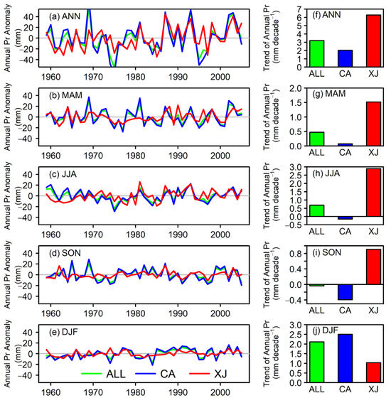
Figure 3.
The inter-annual and long-term trends of precipitation over Arid Central Asia based on the CRU data from 1959 to 2005. The left panel displays the inter-annual variability in precipitation anomalies (relative to the annual mean), while the right panel shows the decadal trends of precipitation. From top to bottom, the rows represent ANN, MAM, JJA, SON, and DJF, respectively. The green color represents the ALL region, the blue color represents the CA region, and the red color represents the XJ region.
Based on the analysis of the monthly climatological data (refer to Figure 4), May stands out as the month with the highest precipitation in the ALL region, reaching 23.06 mm. In comparison, September experienced the lowest precipitation at only 10.53 mm. In the CA and XJ regions, the highest precipitation was observed in April and July, respectively, with values of 26.32 mm and 19.44 mm (Figure 4a). The highest trend of monthly precipitation is observed in December for the ALL and CA regions and June for the XJ region, while September shows the least change (Figure 4b).
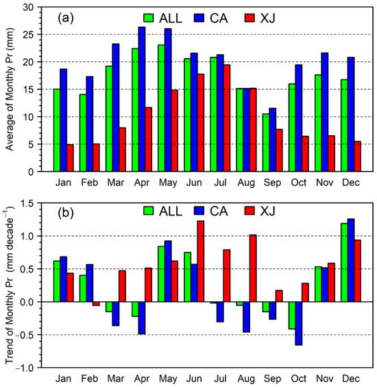
Figure 4.
The climatological monthly precipitation based on the CRU data from 1959 to 2005 over the ALL region. The climatological monthly mean of precipitation (mm) (a); trends of climatological monthly mean of precipitation (mm/decade) (b). The green bar represents the ALL region, the blue bar represents the CA region, and the red bar represents the XJ region.
3.2. Model Evaluation
3.2.1. Evaluation of Mean Annual Precipitation
First, we compared the simulated mean precipitation obtained from the CMIP5 and CMIP6 models with the observational data from the CRU. Notably, substantial spatial heterogeneity is evident on the bias of individual CMIP5 and CMIP6 model simulations, as well as in their MMEs, from 1959 to 2005. This analysis was conducted for the whole year and from seasonal perspectives (Figure 5, Figures S3–S12). Compared with the CRU, 37 out of 43 CMIP5 model simulations exhibit an overestimation of mean annual precipitation in over 90% of the ALL region for ANN (Figure S3). Similarly, 32 out of 43 model simulations overestimate the mean annual precipitation for MAM, 39 out of 43 for SON, and 42 out of 43 for DJF, respectively, in most parts of the ALL region (Figures S4, S6, and S7). Unsurprisingly, this overestimation trend is also observed in the CMIP5 MME (Figure 5), and is particularly pronounced in regions characterized by higher elevations and greater topographical variations, such as the Tien Shan Mountains, the Pamir Plateau, the Altai Mountains, the peripheries of the Qinghai–Tibet Plateau, and the Kazakh hills. However, certain smaller desert regions located in the central part of the ALL region experience an underestimation of precipitation, with up to 110 mm less than the expectation (Figure 5). Additionally, most CMIP5 model simulations indicate an underestimation of mean annual precipitation in more than 90% of the ALL region for JJA (Figure S5). In contrast, the CMIP6 MME exhibits a bias pattern similar to that of the CMIP5 MME for ANN and its four seasons (Figure 5f–j). However, the bias in the CMIP6 MME is significantly reduced, resulting in a decreased proportion of regions with overestimated mean annual precipitation for ANN, MAM, SON, and DJF, reduced to 74.6%, 75.8%, 80.3%, and 83.3%, respectively.
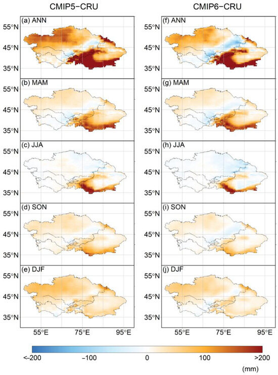
Figure 5.
Spatial pattern of precipitation bias across the ALL region, comparing CRU observations with CMIP5/CMIP6 MME from 1959 to 2005. The left panel displays the bias of the CRU and CMIP5 MME, while the right panel shows the bias of the CRU and CMIP6 MME. The rows from top to bottom represent ANN, MAM, JJA, SON, and DJF, respectively.
Next, we assess the spatial variation in simulated mean annual precipitation. As shown in the Taylor diagrams in Figure 6 and Figure 7, most models generally capture the spatial patterns of mean annual precipitation across the ALL region quite effectively, as evidenced by an r value exceeding 0.6 for most models. However, the magnitude of spatial variability varies widely across models, as indicated by the extensive range of Taylor statistics and TSS values observed across the ALL and its sub-regions during ANN and its four sub-seasons. For example, the r between the simulation results for each model (CMIP5/CMIP6) and their MMEs versus the CRU ranges from 0.30/0.29 to 0.71/0.78. The STD ranges from 1.09/1.00 to 2.95/3.29, the RMSE spans from 39.75/32.71 to 315.94/182.24, and the TSS fluctuates from 0.23/0.13 to 0.69/0.70. Concerning different sub-regions, all model simulations tend to perform less effectively in the XJ region, exhibiting lower TSS values ranging from 0.04/0.03 to 0.39/0.36 (Tables S3 and S4). It is noteworthy that the XJ region has relatively limited performance in simulating mean annual precipitation patterns, which may also be influenced by the scarcity of stations and the complexity of the terrain. Furthermore, the performance of CMIP model simulations also displays significant seasonal variations within each region. For example, the TSS values are significantly higher in winter than in other seasons across the ALL region. In contrast, in the CA region, the TSS values are higher in JJA than in other seasons. Moreover, the ensembles of CMIP model simulations generally exhibit relatively superior performance than most of the individual model simulation results for the ALL region in all seasons. When comparing CMIP6 model simulations with CMIP5 model simulations and their MMEs, it is evident that the TSS values in all regions and seasons are improved in the CMIP6 model simulations, indicating an improvement in the capacity of the CMIP6 model simulation to accurately model annual precipitation.
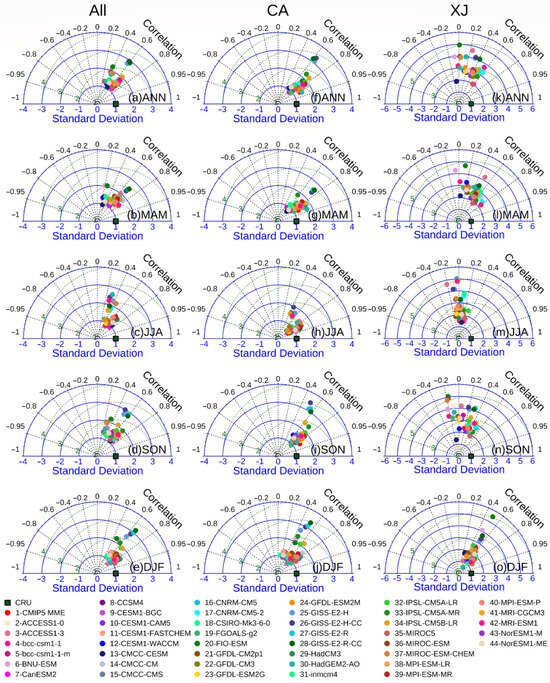
Figure 6.
Taylor diagram comparing CMIP5 model simulation results with observed mean annual precipitation for different seasons in Arid Central Asia. The first column presents comparisons of the ALL region (a–e), CA region (f–j), and XJ region (k–o) in ANN, MAM, JJA, SON, and DJF, respectively. Dots in the figure indicate individual models as well as the MME. Distances from the origin (radius) indicate STD (blue solid lines); radial lines (angles) indicate r values (black dotted lines); and distances from the reference point (CRU, green square in the diagram) indicate RMSEs (green dotted lines).
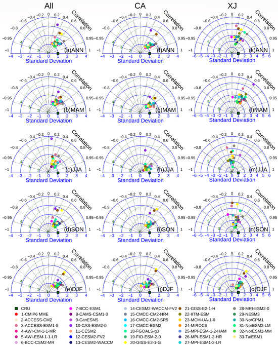
Figure 7.
Taylor diagram comparing CMIP6 model simulation results with observed mean annual precipitation for different seasons in Arid Central Asia. The first column presents comparisons for the ALL region (a–e), CA region (f–j), and XJ region (k–o) in ANN, MAM, JJA, SON, and DJF, respectively. Dots in the figure indicate individual models as well as the MME. Distances from the origin (radius) indicate STD (blue solid lines); radial lines (angles) indicate r values (black dotted lines); and distances from the reference point (CRU, green square in the diagram) indicate RMSEs (green dotted lines).
3.2.2. Inter-Annual Variability and Annual Trends
This section assesses the ability of CMIP model-simulated precipitation to capture alterations in CRU data over time, encompassing inter-annual fluctuations and long-term trends. Our findings suggest that the simulated precipitation generally succeeds in reproducing the observed pattern of inter-annual precipitation variability across the ALL region during all four seasons. Positive r values were identified in nearly all model simulations, with median r values typically exceeding 0.5 (Figure 8 and Figure 9). In the CA region, the simulated precipitation from the CMIP model simulations reasonably captured the observed patterns of inter-annual precipitation variability, with the majority of simulations yielding a median r value above 0.6 (Figure 8 and Figure 9). However, the performance of all the CMIP model simulations in capturing the inter-annual precipitation variability of the CRU in the XJ regions varied considerably for all seasons, with most simulations displaying a median r lower than 0.5 (Figure 8 and Figure 9).
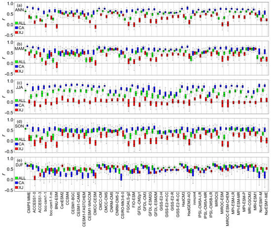
Figure 8.
Evaluation of the simulated inter-annual variability in precipitation across the ALL region from 1959 to 2005 for the CMIP5 models. Box plot of r between the observed and simulated annual precipitation. The rows from top to bottom represent ANN, MAM, JJA, SON, and DJF, respectively. Green, blue, and red represent the ALL region, CA region, and XJ region, respectively. In each plot, boxes indicate the 25th and 75th percentiles and whiskers represent the minimum and maximum values of all catchments. The median value is shown as a dark horizontal line inside each box.
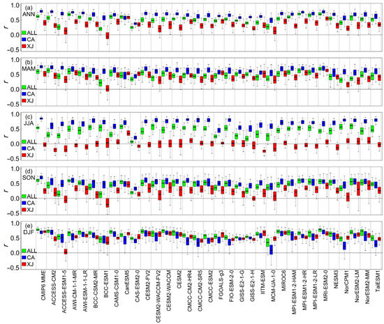
Figure 9.
Evaluation of the simulated inter-annual variability of precipitation across the ALL region from 1959 to 2005 for the CMIP6 models. Box plot of r between the observed and simulated annual precipitation. The rows from top to bottom represent ANN, MAM, JJA, SON, and DJF, respectively. Green, blue, and red represent the ALL region, CA region, and XJ region, respectively. In each plot, boxes indicate the 25th and 75th percentiles and whiskers represent the minimum and maximum values of all catchments. The median value is shown as a dark horizontal line inside each box.
A comparison of the mean annual precipitation trend between CMIP model simulations and the CRU for ANN and its four seasons is shown in Figure 10 and Figure 11. From 1959 to 2005, the CRU mean annual precipitation displayed an overall positive trend across the ALL region of 3.18 ± 0.60 mm/decade, 0.63 ± 0.23 mm/decade, 0.68 ± 0.29 mm/decade, 0.26 ± 0.20 mm/decade, and 1.77 ± 0.23 mm/decade in ANN, MAM, JJA, SON, and DJF, respectively (median ± one STD).
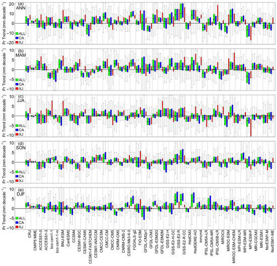
Figure 10.
Evaluation of the simulated annual precipitation trend across the ALL region from 1959 to 2005 for the CMIP5 models. Box plot of the observed and simulated annual precipitation trends. The rows from top to bottom represent ANN, MAM, JJA, SON, and DJF, respectively. Green, blue, and red represent the ALL region, CA region, and XJ region, respectively. In each plot, boxes indicate the 25th and 75th percentiles and whiskers represent the minimum and maximum values of all catchments. The median value is shown as a dark horizontal line inside each box.
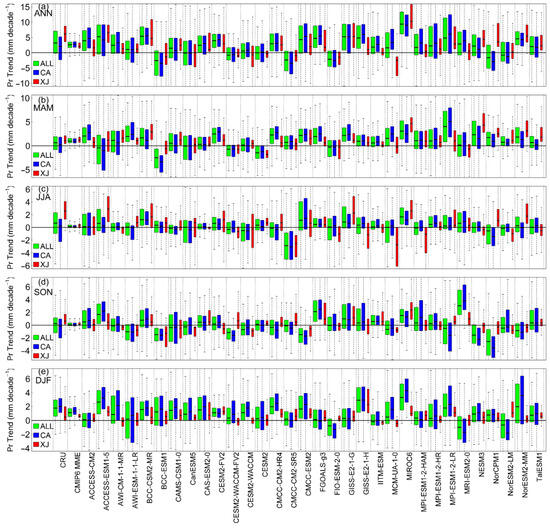
Figure 11.
Evaluation of the simulated annual precipitation trend across the ALL region from 1959 to 2005 for the CMIP6 models. Box plot of the observed and simulated annual precipitation trends. The rows from top to bottom represent ANN, MAM, JJA, SON, and DJF, respectively. Green, blue, and red represent the ALL region, CA region, and XJ region, respectively. In each plot, boxes indicate the 25th and 75th percentiles and whiskers represent the minimum and maximum values of all catchments. The median value is shown as a dark horizontal line inside each box.
3.2.3. Intra-Annual Cycle of Precipitation
We evaluated intra-annual precipitation cycles by comparing monthly climatological precipitation between the CRU and model simulations throughout the year. Figure 12 demonstrates that the CMIP model simulations generally captured the intra-annual cycle of precipitation from CRU but exhibited an initial bias in the timing of peak monthly precipitation. In contrast, the timing of minimum monthly precipitation was reasonably simulated in September for all the CMIP model simulations in the ALL and CA regions (Figure 12a–c). Regarding trends in the intra-annual precipitation cycle changes, there are contrasting trends between the CMIP model-simulated and observed precipitation in the ALL and its sub-regions in individual months. This contrast is notable in March, April, August, and October in the ALL and CA regions and in February, July, and November in the XJ region (Figure 12d–f).
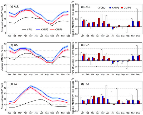
Figure 12.
Comparison of the MME simulation results from CMIP5 and CMIP6 with the time series of monthly precipitation observed by the CRU from 1959 to 2005. The left panel displays the time series of the monthly average precipitation (mm), while the right panel shows the trend of the monthly average precipitation (mm/decade). The rows from top to bottom correspond to ALL, CA, and XJ, respectively. The black line represents the CRU observation, the blue line represents the CMIP5 MME, and the red line represents the CMIP6 MME.
Figure 13 and Figure 14 depict significant variability in monthly climatological precipitation in the CMIP5 and CMIP6 model simulations for the ALL region and its sub-regions. Specifically, most model simulations in both CMIP5 and CMIP6 overestimated the precipitation in the ALL region and its sub-regions during MAM, SON, and DJF. Conversely, most model simulations in CMIP5 and CMIP6 underestimated the precipitation in the ALL region and its sub-regions during JJA. Notably, the AEs for CMIP6 MME (MAM, SON, and DJF are 9.12–10.83 mm, 3.03–7.92 mm, and 8.79–9.84 mm, respectively) are closer to the CRU than those from the AE for CMIP5 MME (11.51–12.21 mm, 6.35–12.01 mm, and 12.33–14.57 mm) over the ALL region and its sub-regions. However, there is an evident exception in the CA region during JJA, where a slight overestimation is observed in the CMIP5 MME and vice versa in the CMIP6 MME. For example, the overestimation of the CMIP5 MME during JJA in the CA region ranges from 2.5% to 18.9%, while the underestimation of CMIP6 MME during JJA in the CA region ranges from −0.8% to −15.1%.
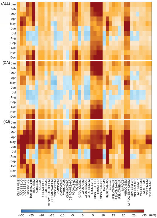
Figure 13.
Bias heatmap of the monthly climatological precipitation of each CMIP5 model simulation and CMIP5 MME compared with observed data across the ALL region and its sub-regions from 1959 to 2005.
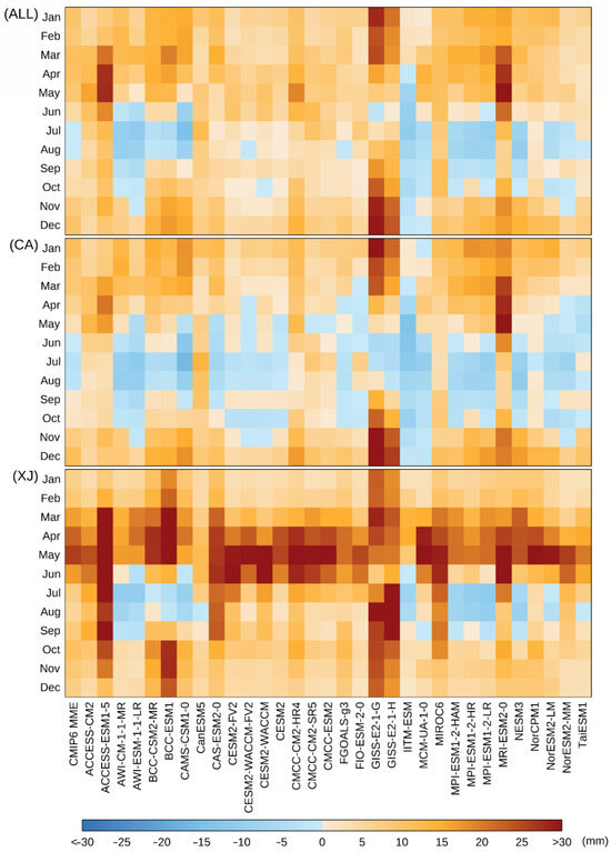
Figure 14.
Bias heatmap of the monthly climatological precipitation of each CMIP6 model simulation and CMIP6 MME compared with observed data across the ALL region and its sub-regions from 1959 to 2005.
3.2.4. Evaluation of Overall Model Performance
This section concentrates on quantitatively assessing the overall performance of models in simulating annual precipitation using the CRI method (Figure 15). For the ALL region (Figure 15a,d,g,j,m), in all seasons except DJF, half or more of the institutions in CMIP6 showed higher CRI values compared to CMIP5. The most significant improvement was seen in FIO during the MAM (CRI values of 0.09 for CMIP5 and 0.7 for CMIP6). As for different sub-regions, only in JJA for the CA region and JJA for the XJ region did the CRI values of the CMIP6 institutions surpass those of CMIP5 (Figure 15h,i). Additionally, it is noteworthy that in CMIP5 and CMIP6, most individual institutions performed significantly better in terms of MME. However, the CRI values from the ensembles of the CMIP6 institutions performed similarly and considerably better than the CMIP5 ensembles, except in the CA region during ANN, SON, and DJF, and in the XJ region during ANN and SON. Moreover, for the MMEs, the most substantial improvement was observed during JJA for the ALL region, where the CRI value for CMIP6 MME was 0.76, significantly higher than the CMIP5 MME value of 0.58 (Figure 15g).
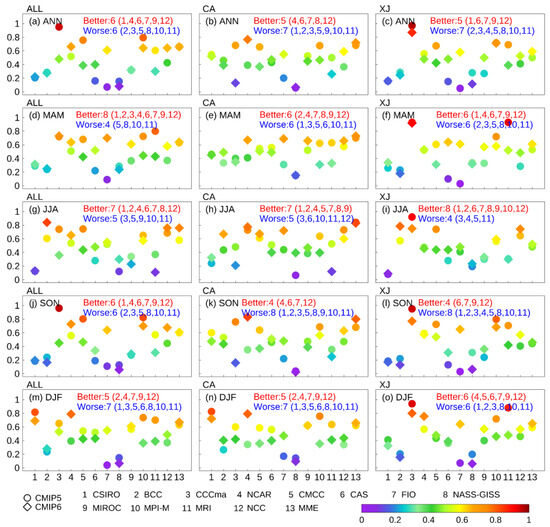
Figure 15.
CRI statistics are available for the complete ALL region and its sub-regions, simulated by both the CMIP5 and CMIP6 models, along with their Multi-Model Ensemble (MME) counterparts across various institutions. The CRI value for each institution was derived from the arithmetic mean of the CRI values calculated for their respective simulation models. Circles and diamonds denote CMIP5 and CMIP6 organizations, respectively.
3.3. Predicted Precipitation Changes in Future Forecasts
3.3.1. Spatial Pattern of Average Annual Precipitation from 2054 to 2100
Figure 16 and Figure 17 depict the spatial patterns of the mean annual precipitation changes projected by the CMIP5 and CMIP6 models under three scenarios from 2054 to 2100 compared to the baseline of 1959–2005. In the CMIP5 MME simulations, the projected mean annual precipitation for ANN under different scenarios exhibits a widespread increase across the ALL region, with maximum changes relative to the historical period of 108.26 mm, 134.93 mm, and 216.74 mm, respectively. This increase is particularly prominent at the Pamir Plateau, Tien Shan Mountain, the periphery of the Tibetan Plateau, and the northern part of the CA region. However, a reduction in simulated precipitation is observed in the southwestern part of the CA region. When considering different seasons, the spatial pattern of precipitation variability during MAM and DJF largely mirrors that of ANN. In contrast, during JJA, a noticeable decreasing trend in precipitation is observed in the southern areas of the CA region, with maximum changes of −5.86 mm, −10.83 mm, and −13.07 mm under the three scenarios. Additionally, the northern part of the CA region and the western and southern parts of the XJ region appear to show an increase in precipitation changes.
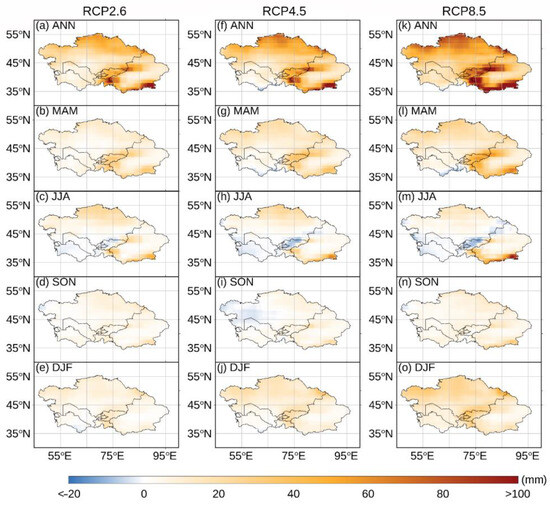
Figure 16.
The spatial pattern of precipitation changes under various future scenarios for the future period (2054–2100) compared to the historical period (1959–2005). The left, middle, and right columns show the spatial distribution of precipitation alterations within the context of the RCP 2.6, RCP 4.5, and RCP 8.5 scenarios, respectively. The rows from top to bottom are ANN, MAM, JJA, SON, and DJF, respectively.
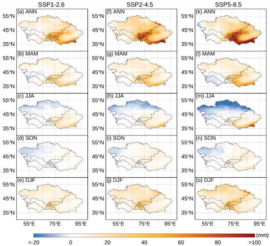
Figure 17.
The spatial pattern of precipitation changes under various future scenarios for the future period (2054–2100) compared to the historical period (1959–2005). The left, middle, and right columns show the spatial distribution of precipitation alterations within the context of the SSP1-2.6, SSP2-4.5, and SSP5-8.5 scenarios, respectively. The rows from top to the bottom are ANN, MAM, JJA, SON, and DJF, respectively.
Similar to CMIP5, the CMIP6 MME simulations also indicate an increase in future precipitation changes in ANN, MAM, and DJF under different scenarios (Figure 17). However, a significant decrease in future precipitation changes is observed within the northern part of the CA region during JJA, which accounts for nearly 60% of the ALL region. The remaining regions show minor changes compared to the historical period, except for some increases in the western and southern parts of the XJ region. During SON, the relative changes in future precipitation across the ALL region are minimal, with a slight decrease in the western part of the CA region and slight increases in other regions. Moreover, the relative change between the two periods becomes increasingly significant with higher emission concentrations. For example, the mean annual precipitation changes during MAM, as simulated by the CMIP5 MME, show an 11.8% increase in the ALL region under the low-emissions scenarios (RCP 2.6) and under the high-emissions scenario (RCP 8.5), and the CMIP5 MME has a 22.3% increase in average annual precipitation. Additionally, compared to the RCP 2.6 scenario, the area with increased precipitation remains largely unchanged (from 99.9% to 99.1%) under the SSP1-2.6 scenario. In the medium-emissions scenarios, the area with increased precipitation increases (RCP 4.5/SSP2-4.5: 98.7%/100%), while it decreases under the high-emissions scenarios (RCP 8.5/SSP5-8.5: 99.7%/96.2%) in ANN (Figure 16 and Figure 17).
3.3.2. Inter-Annual Variability and Long-Term Trend in Mean Annual Precipitation in the Future
Based on the inter-annual variability and long-term trends in mean annual precipitation anomalies from 1959 to 2100 (Figure 18 and Figure 19), the mean annual precipitation in ANN, MAM, SON, and DJF generally shows a fluctuating increase across the ALL region and its sub-regions under different scenarios; however, the mean annual precipitation during JJA shows a fluctuating decrease across the ALL region and its sub-regions under different scenarios. Additionally, the long-term precipitation changes under different scenarios (RCPs or SSPs) remain relatively consistent until 2050, after which they significantly diverge. Similarly, beyond 2050, the future precipitation trends vary considerably by sub-region under different emission scenarios, closely resembling the patterns observed in the ALL region. Notably, the most significant increasing trends in ANN precipitation occur predominantly in the XJ region, with approximately 1.64 mm/decade and 1.40 mm/decade under the RCP 2.6 and SSP1-2.6 scenarios, and 2.59 mm/decade and 3.85 mm/decade under the RCP 4.5 and SSP2-4.5 scenarios. It is important to highlight that the CA region displays a decreasing trend in precipitation in JJA under the RCP 8.5 and SSP5-8.5 scenarios, with trends of −0.23 mm/decade and −1.66 mm/decade, respectively. Comparing the precipitation changes of the CMIP5 and CMIP6 model simulations under the same emissions scenarios reveals that the changing trend of precipitation in the SSPs consistently exceeded that in the RCPs in the XJ region during different seasons under all scenarios, except during SON and DJF under the RCP 2.6 and SSP1-2.6 scenarios. In contrast, in the CA region, the change trend in the RCPs generally surpassed that in the SSPs, except during the JJA season under the RCP 8.5 and SSP5-8.5 scenarios, as well as the SON season under the RCP 2.6 and SSP1-2.6 scenarios.
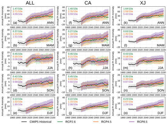
Figure 18.
Temporal evolution of precipitation anomalies as simulated by the CMIP5 models covering the entire ALL region and its respective sub-regions from 1959 to 2100. The shaded areas indicate one STD range across different scenarios; the rows from top to the bottom are ANN, MAM, JJA, SON, and DJF, respectively.
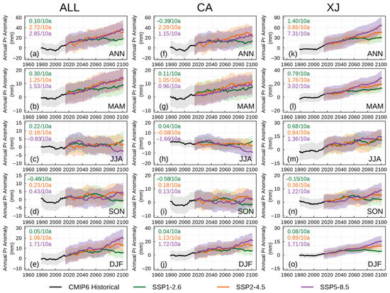
Figure 19.
Temporal evolution of precipitation anomalies as simulated by the CMIP6 models covering the entire ALL region and its respective sub-regions from 1959 to 2100. The shaded areas indicate one STD range across different scenarios; the rows from top to the bottom are ANN, MAM, JJA, SON, and DJF, respectively.
4. Discussion
Globally/regionally simulated precipitation has been widely used in analyses of weather/hydrological extremes and assessments of historical and future changes in precipitation at global and/or regional scales [73,74]. Since precipitation is related to water resource management [75], flood and drought risk mitigation [76], ecological security [77], economic development [78], and other related fields, it is important that we have good estimates of how likely this precipitation is to occur and whether that likelihood is changing.
This study extensively examined the performance of two generations of state-of-the-art CMIP model simulations in replicating precipitation changes (mean annual, inter-annual variability, and monthly climatology) over the Arid Central Asia region against CRU data. Our comprehensive analysis reveals that neither CMIP5 nor CMIP6 model simulations satisfactorily capture all aspects of the temporal and spatial characteristics of the CRU data across the entire ALL region and its two sub-regions. Moreover, most institutions employing CMIP6 showed CRI values that were lower or closer to the reference than those using CMIP5 for both the ALL region and its sub-regions in certain seasons, which is contrary to recent studies that have suggested overall improvements in the precipitation change simulations in CMIP6 models on a global scale [79,80]. Specifically, we observed that most model simulations tend to overestimate the magnitude of mean annual precipitation in the ALL region across all four seasons. This suggests that these models may exaggerate the annual variation in water flux, and, as a consequence, the risks associated with extreme precipitation, as assessed using these model outputs, could be overestimated. Additionally, we found that only 70% of the models correctly capture the observed sign of annual precipitation trends, and the models examined herein were found to overestimate the simulated precipitation trend over the ALL region, especially in XJ. Our above evaluation results suggest that there is large uncertainty in predicting the changing direction of wetness/humidity changes or extreme weather/hydrological events over time based on these model outputs. As for the intra-annual variability, most models exhibit an early bias in the timing of maximum monthly precipitation (Figure 12). Biases in the timing of maximum monthly precipitation directly lead to biased predictions of the onset of flood events or crop yield, even seasonal peaks of vegetation photosynthesis, bringing additional challenges for disaster warning and prevention and ecological security. In terms of future precipitation changes over the ALL region, we found an increasing precipitation trend in XJ for all seasons and a decreasing precipitation trend in summer in the CA region. Given the mounting evidence suggesting intensification of the warming and moistening phenomenon in the northwest of China [81,82], it is likely to significantly alleviate water scarcity, promote socio-economic development, and enhance the ecological environment in this region [81,83]. In addition, under the high-emission scenario (RCP 8.5/SSP5-8.5), due to the warming effect caused by greenhouse gas emissions, the decreasing precipitation trend in summer in the CA region may further intensify metrological/agricultural/hydrological drought in CA in the future [84,85].
This study highlights that source bias in the latest, cutting-edge CMIP6 model simulations can be attributed to three primary factors: topographic effects, model structure or parameterizations, and spatial resolution [86,87,88]. First, the CMIP model simulations exhibited higher precipitation compared to the CRU data, indicating a noticeable wet bias in the CMIP model simulations over the ALL region. This wet bias was evident in the CMIP6 model simulations and particularly pronounced in high-altitude regions with complex terrains, such as the Pamir Plateau, Kunlun Mountains, Tien Shan Mountains, and Altai Mountains during the MAM, SON, and DJF seasons. Previous studies reported that local convective processes (i.e., valley winds and orographic rainfall) typically influence precipitation changes in the ALL region because of its intricate topography [89,90,91]. An isotope hydrology study in the Qilian Mountains and Hexi Corridor showed that indigenous moisture recycling contributed to 24% of the total precipitation in the upstream regions during the period from May to September. Although topographic corrections yield improvements in gridded precipitation performance (nearly 20%) [92], the model’s capacity to faithfully replicate precipitation across intricate terrains over the ALL region (particularly the Xinjiang or XJ region) remains inadequate. This insufficiency arises due to the incomplete consideration of topographic corrections in the CMIP6 model simulations [27], leading to substantial deviations in mean annual precipitation simulations, as observed by Hernandez et al. [79].
Second, improving the simulation of zonal/latitudinal water vapor flux convergence in the model parameterizations has the potential to improve the models’ abilities to simulate precipitation changes [93]. For example, Yang et al. [94], through a moisture budget analysis, indicated that the wet bias of simulated winter precipitation is primarily linked to the overestimation of evaporation. In this study, we showed that the CMIP model exhibited generally improved performance during the summer season compared to early spring and late winter. This variance in performance could be attributed to variations in the models’ capacity to simulate water vapor in different seasons. Furthermore, an early bias in the timing of the rainy season was observed for CMIP model simulations, which could partly be attributed to difficulties in correctly reproducing seasonal meridional shifts in the subtropical westerly jet (e.g., the South Atlantic Ocean). In addition, during early spring and late winter, intricate air–sea interactions and teleconnections exist, which might not be adequately captured by current general circulation models. This suggests a need for further enhancements and refinements in the future to better represent these processes.
The third uncertainty in our assessment arises from the coarse spatial resolution of the global models (especially the CMIP6 model). For example, as shown in Tables S1 and S2, CMIP6 model simulations at the CMCC, MRI, and MPI-M institutes have higher spatial resolution compared to CMIP5. However, the model performance of CMIP6 in these three institutions to simulate precipitation variability in the ALL region was worse compared to CMIP5 (Figure 16a).
It is often reported that MMEs outperform single-model simulations [95,96,97]. Our analysis indicates that simple averages generally exhibit superior performance compared to most individual model simulations across all evaluated aspects. Nevertheless, the constraints associated with simple averages in comprehensively representing all three aspects of our study in certain regions suggest that the straightforward ensemble mean method might not be appropriate for evaluating particular areas. This underscores the potential effectiveness of more intricate multi-model ensemble approaches, such as Bayesian averages [98] or weighted averages [99], as alternatives to simple averages.
5. Conclusions
This study evaluates the ability of CMIP5 and CMIP6 model simulations and their MMEs to simulate precipitation and predict future changes in the ALL region and its two sub-regions for all seasons under RCPs and SSPs, using CRU data as a baseline. Each model simulation was assessed in terms of mean annual magnitude, inter-annual variability, long-term trends, and the seasonal cycle, and the main findings are summarized as follows:
- (1)
- The mean annual precipitation in the ALL region during the four seasons was generally overestimated. However, an unexpected underestimation was observed in the CA region during the JJA. The CMIP model simulations performed reasonably well in capturing the CRU precipitation variability. However, none of the models satisfactorily reproduced the trends in precipitation, with only 70% of models correctly simulating the observed sign of annual precipitation trends. In addition, the spatial variability of the estimated annual precipitation trends was only moderately consistent (r > 0.5) with observations in the MAM and JJA time periods in the CA region. and poorly consistent with the observation in the XJ region (r < 0.4).
- (2)
- All models demonstrated a fairly accurate representation of the CRU’s seasonal precipitation patterns. However, most models tended to overestimate the intra-annual precipitation variability and demonstrated a bias toward the early occurrence of maximum monthly precipitation.
- (3)
- Regarding the holistic evaluation, within the ALL region, the majority of institutions employing the CMIP6 model exhibited higher CRI values compared to those utilizing the CMIP5 model. There were more institutions with “better” simulation abilities from CMIP6 than those with “worse” abilities across the ALL region and its sub-regions during specific seasons. Conversely, in the CA region during SON and DJF, and in the XJ region during SON, there were more institutions with “worse” simulation abilities using CMIP6 compared to “better” ones.
- (4)
- Consistent with many previous findings, in general, the simple average multi-model ensembles effectively improved model performance compared to most of the individual models. However, we found that the ensemble of the CMIP5 and CMIP6 models performed worse than most individual CMIP5 and CMIP6 models in simulating mean annual precipitation in the CA region during MAM, SON, and DJF; inter-annual variability and intra-annual variability in DJF precipitation in the XJ region; and the MAM precipitation trend in the XJ region.
- (5)
- The projections indicated a future increase in precipitation over the ALL region from 1959 to 2100, particularly in the XJ region. The models with better simulation abilities predicted an increasing trend over the ALL region from 2006 to 2100, except for the CA region during JJA. However, the CMIP5 and CMIP6 scenarios exhibited no significant difference until 2050, and then, rapidly diverged. It is worth noting that under the same emission scenarios, the CMIP6 model simulations resulted in stronger precipitation trends compared to CMIP5, especially in the XJ region.
Supplementary Materials
The following supporting information can be downloaded at: https://www.mdpi.com/article/10.3390/rs15235460/s1. Figure S1: Map of CRU data site locations. Figure S2: Fitted plot between CRU data and MSWEP data. Figure S3: Spatial distribution of precipitation bias between CRU observations and CMIP5 models for ANN from 1959 to 2005. Figure S4: Same as Figure S3 but for MAM. Figure S5: Same as Figure S3 but for JJA. Figure S6: Same as Figure S3 but for SON. Figure S7: Same as Figure S3 but for DJF. Figure S8: Spatial distribution of precipitation bias between CRU observations and CMIP6 models for ANN from 1959 to 2005. Figure S9: Same as Figure S8 but for MAM. Figure S10: Same as Figure S8 but for JJA. Figure S11: Same as Figure S8 but for SON. Figure S12: Same as Figure S8 but for DJF. Table S1: Summary of CMIP5 models used in this study. Table S2: Summary of CMIP6 models used in this study. Table S3: TSS of MME and each model under CMIP5. ALL, CA, and XJ represent the entire study area, the five Central Asian countries, and the Xinjiang region, respectively. ANN, MAM, JJA, SON, and DJF represent the annual average, spring, summer, autumn, and winter precipitation, respectively. The highest and lowest TSS values for MME and each GCM are shown in bold and underlined, respectively. Table S4: TSS of MME and each model under CMIP6. ALL, CA, and XJ represent the entire study area, the five Central Asian countries, and the Xinjiang region, respectively. ANN, MAM, JJA, SON, and DJF represent the annual average, spring, summer, autumn, and winter precipitation, respectively. The highest and lowest TSS values for MME and each GCM are shown in bold and underlined, respectively.
Author Contributions
Visualization, conceptualization, data curation, methodology, writing—original draft preparation, B.X.; conceptualization, supervision, methodology, writing—review and editing, H.G.; supervision, resources, funding acquisition, F.M.; supervision, project administration, funding acquisition, C.S.; investigation, supervision, inspection, funding acquisition, M.L. All authors have read and agreed to the published version of the manuscript.
Funding
This work was jointly supported by the National Natural Science Foundation of China (42101030, 42261079, 42361024), the Key Research, Development and Achievement Transformation Project of Inner Mongolia Autonomous Region (2022YFDZ0061), the Third Xinjiang Scientific Expedition Program (2021xjkk1400), the Talent Project of Science and Technology in Inner Mongolia (NJYT23019, NJYT22027), the Project of the Natural Science Foundation of Inner Mongolia (2022MS04004), Fundamental Research Funds for the Inner Mongolia Normal University (2022JBBJ014, 2022JBQN093, 2023JBPT004) and the Master’s Degree Research and Innovation Program Fund of Inner Mongolia Autonomous Region (S20231080Z).
Data Availability Statement
No new data were created for this paper. The data in the paper were downloaded from the address provided in the Data section and calculated using the formulas in the paper.
Conflicts of Interest
The authors declare no conflict of interest.
References
- Ougahi, J.H.; Cutler, M.E.J.; Cook, S.J. Modelling climate change impact on water resources of the Upper Indus Basin. J. Water Clim. Chang. 2021, 13, 482–504. [Google Scholar] [CrossRef]
- Gherardi, L.A.; Sala, O.E. Effect of interannual precipitation variability on dryland productivity: A global synthesis. Glob. Chang. Biol. 2019, 25, 269–276. [Google Scholar] [CrossRef] [PubMed]
- Weltzin, J.F.; Loik, M.E.; Schwinning, S.; Williams, D.G.; Fay, P.A.; Haddad, B.M.; Harte, J.; Huxman, T.E.; Knapp, A.K.; Lin, G.; et al. Assessing the Response of Terrestrial Ecosystems to Potential Changes in Precipitation. BioScience 2003, 53, 941–952. [Google Scholar] [CrossRef]
- Aghapour Sabbaghi, M.; Nazari, M.; Araghinejad, S.; Soufizadeh, S. Economic impacts of climate change on water resources and agriculture in Zayandehroud river basin in Iran. Agric. Water Manag. 2020, 241, 106323. [Google Scholar] [CrossRef]
- Zhang, W.; Zhou, T.; Zhang, L.; Zou, L. Future Intensification of the Water Cycle with an Enhanced Annual Cycle over Global Land Monsoon Regions. J. Clim. 2019, 32, 5437–5452. [Google Scholar] [CrossRef]
- Li, B.; Chen, Y.; Shi, X.; Chen, Z.; Li, W. Temperature and precipitation changes in different environments in the arid region of northwest China. Theor. Appl. Climatol. 2013, 112, 589–596. [Google Scholar] [CrossRef]
- Gu, G.; Adler, R.F. Observed variability and trends in global precipitation during 1979–2020. Clim. Dyn. 2023, 61, 131–150. [Google Scholar] [CrossRef]
- Carvalho, L.M.V. Assessing precipitation trends in the Americas with historical data: A review. WIREs Clim. Chang. 2020, 11, e627. [Google Scholar] [CrossRef]
- Sun, Q.; Miao, C.; Duan, Q.; Ashouri, H.; Sorooshian, S.; Hsu, K.-L. A Review of Global Precipitation Data Sets: Data Sources, Estimation, and Intercomparisons. Rev. Geophys. 2018, 56, 79–107. [Google Scholar] [CrossRef]
- Koutsouris, A.J.; Seibert, J.; Lyon, S.W. Utilization of Global Precipitation Datasets in Data Limited Regions: A Case Study of Kilombero Valley, Tanzania. Atmosphere 2017, 8, 246. [Google Scholar] [CrossRef]
- Scafetta, N. CMIP6 GCM ensemble members versus global surface temperatures. Clim. Dyn. 2023, 60, 3091–3120. [Google Scholar] [CrossRef]
- Siabi, E.K.; Kabobah, A.T.; Akpoti, K.; Anornu, G.K.; Amo-Boateng, M.; Nyantakyi, E.K. Statistical downscaling of global circulation models to assess future climate changes in the Black Volta basin of Ghana. Environ. Chall. 2021, 5, 100299. [Google Scholar] [CrossRef]
- Xiang, Y.; Wang, Y.; Chen, Y.; Zhang, Q. Impact of Climate Change on the Hydrological Regime of the Yarkant River Basin, China: An Assessment Using Three SSP Scenarios of CMIP6 GCMs. Remote Sens. 2022, 14, 115. [Google Scholar] [CrossRef]
- Lalande, M.; Ménégoz, M.; Krinner, G.; Naegeli, K.; Wunderle, S. Climate change in the High Mountain Asia in CMIP6. Earth Syst. Dyn. 2021, 12, 1061–1098. [Google Scholar] [CrossRef]
- Taylor, K.E.; Stouffer, R.J.; Meehl, G.A. An Overview of CMIP5 and the Experiment Design. Bull. Am. Meteorol. Soc. 2012, 93, 485–498. [Google Scholar] [CrossRef]
- Liu, Z.; Mehran, A.; Phillips, T.J.; Aghakouchak, A. Seasonal and regional biases in CMIP5 precipitation simulations. Clim. Res. 2014, 60, 35–50. [Google Scholar] [CrossRef]
- Yang, X.; Yong, B.; Yu, Z.; Zhang, Y. An evaluation of CMIP5 precipitation simulations using ground observations over ten river basins in China. Hydrol. Res. 2021, 52, 676–698. [Google Scholar] [CrossRef]
- Moss, R.H.; Edmonds, J.A.; Hibbard, K.A.; Manning, M.R.; Rose, S.K.; van Vuuren, D.P.; Carter, T.R.; Emori, S.; Kainuma, M.; Kram, T.; et al. The next generation of scenarios for climate change research and assessment. Nature 2010, 463, 747–756. [Google Scholar] [CrossRef]
- Chen, J.; Arsenault, R.; Brissette, F.P.; Zhang, S. Climate Change Impact Studies: Should We Bias Correct Climate Model Outputs or Post-Process Impact Model Outputs? Water Resour. Res. 2021, 57, e2020WR028638. [Google Scholar] [CrossRef]
- Kim, S.; Park, S.; Shin, J. Impact of Subgrid Variation of Water Vapor on Longwave Radiation in a General Circulation Model. J. Adv. Model. Earth Syst. 2020, 12, e2019MS001926. [Google Scholar] [CrossRef]
- Li, J.; Bao, Q.; Liu, Y.; Wang, L.; Yang, J.; Wu, G.; Wu, X.; He, B.; Wang, X.; Zhang, X.; et al. Effect of horizontal resolution on the simulation of tropical cyclones in the Chinese Academy of Sciences FGOALS-f3 climate system model. Geosci. Model Dev. 2021, 14, 6113–6133. [Google Scholar] [CrossRef]
- Long, S.-M.; Li, G. Model Uncertainty in the Projected Indian Summer Monsoon Precipitation Change under Low-Emission Scenarios. Atmosphere 2021, 12, 248. [Google Scholar] [CrossRef]
- Shen, Z.; Sridhar, A.; Tan, Z.; Jaruga, A.; Schneider, T. A Library of Large-eddy Simulations for Calibrating Cloud Parameterizations. ESS Open Arch. 2021, 2021, A55K-1534. [Google Scholar]
- Agel, L.; Barlow, M.; Polonia, J.; Coe, D. Simulation of Northeast U.S. Extreme Precipitation and Its Associated Circulation by CMIP5 Models. J. Clim. 2020, 33, 9817–9834. [Google Scholar] [CrossRef]
- Ayugi, B.; Zhihong, J.; Zhu, H.; Ngoma, H.; Babaousmail, H.; Rizwan, K.; Dike, V. Comparison of CMIP6 and CMIP5 models in simulating mean and extreme precipitation over East Africa. Int. J. Climatol. 2021, 41, 6474–6496. [Google Scholar] [CrossRef]
- Bador, M.; Donat, M.G.; Geoffroy, O.; Alexander, L.V. Assessing the Robustness of Future Extreme Precipitation Intensification in the CMIP5 Ensemble. J. Clim. 2018, 31, 6505–6525. [Google Scholar] [CrossRef]
- Eyring, V.; Bony, S.; Meehl, G.A.; Senior, C.A.; Stevens, B.; Stouffer, R.J.; Taylor, K.E. Overview of the Coupled Model Intercomparison Project Phase 6 (CMIP6) experimental design and organization. Geosci. Model Dev. 2016, 9, 1937–1958. [Google Scholar] [CrossRef]
- Carlson, D.; Eyring, V. Contributions to Climate Science of the Coupled Model Intercomparison Project. Bull./World Meteorol. Organ. (WMO) 2016, 65, 53–56. [Google Scholar]
- Du, Y.; Wang, D.; Zhu, J.; Wang, D.; Qi, X.; Cai, J. Comprehensive assessment of CMIP5 and CMIP6 models in simulating and projecting precipitation over the global land. Int. J. Climatol. 2022, 42, 6859–6875. [Google Scholar] [CrossRef]
- Shiru, M.S.; Shahid, S.; Chae, S.-T.; Chung, E.-S. Replicability of Annual and Seasonal Precipitation by CMIP5 and CMIP6 GCMs over East Asia. KSCE J. Civ. Eng. 2022, 26, 1978–1989. [Google Scholar] [CrossRef]
- Lun, Y.; Liu, L.; Cheng, L.; Li, X.; Li, H.; Xu, Z. Assessment of GCMs simulation performance for precipitation and temperature from CMIP5 to CMIP6 over the Tibetan Plateau. Int. J. Climatol. 2021, 41, 3994–4018. [Google Scholar] [CrossRef]
- Yao, J.; Chen, Y.; Chen, J.; Zhao, Y.; Tuoliewubieke, D.; Li, J.; Yang, L.; Mao, W. Intensification of extreme precipitation in arid Central Asia. J. Hydrol. 2021, 598, 125760. [Google Scholar] [CrossRef]
- Zou, S.; Abuduwaili, J.; Duan, W.; Ding, J.; De Maeyer, P.; Van De Voorde, T.; Ma, L. Attribution of changes in the trend and temporal non-uniformity of extreme precipitation events in Central Asia. Sci. Rep. 2021, 11, 15032. [Google Scholar] [CrossRef] [PubMed]
- Liang-Liang, L.; Jian, L.; Ru-Cong, Y. Evaluation of CMIP6 HighResMIP models in simulating precipitation over Central Asia. Adv. Clim. Chang. Res. 2022, 13, 1–13. [Google Scholar] [CrossRef]
- Dong, T.; Dong, W. Evaluation of extreme precipitation over Asia in CMIP6 models. Clim. Dyn. 2021, 57, 1751–1769. [Google Scholar] [CrossRef]
- Ta, Z.; Yu, Y.; Sun, L.; Chen, X.; Mu, G.; Yu, R. Assessment of Precipitation Simulations in Central Asia by CMIP5 Climate Models. Water 2018, 10, 1516. [Google Scholar] [CrossRef]
- Guo, H.; Bao, A.; Chen, T.; Zheng, G.; Wang, Y.; Jiang, L.; De Maeyer, P. Assessment of CMIP6 in simulating precipitation over arid Central Asia. Atmos. Res. 2021, 252, 105451. [Google Scholar] [CrossRef]
- Zhang, X.; Hua, L.; Jiang, D. Assessment of CMIP6 model performance for temperature and precipitation in Xinjiang, China. Atmos. Ocean. Sci. Lett. 2022, 15, 100128. [Google Scholar] [CrossRef]
- Choudhury, B.A.; Rajesh, P.V.; Zahan, Y.; Goswami, B.N. Evolution of the Indian summer monsoon rainfall simulations from CMIP3 to CMIP6 models. Clim. Dyn. 2022, 58, 2637–2662. [Google Scholar] [CrossRef]
- Vicente-Serrano, S.M.; Maillard, O.; Peña-Angulo, D.; Domínguez-Castro, F.; Noguera, I.; Lorenzo-Lacruz, J.; Azorin-Molina, C.; Juez, C.; Guijarro, J.A.; Halifa-Marín, A.; et al. Evaluation of long-term changes in precipitation over Bolivia based on observations and Coupled Model Intercomparison Project models. Int. J. Climatol. 2023, 43, 1431–1447. [Google Scholar] [CrossRef]
- Liu, L.; Peng, J.; Li, G.; Guan, J.; Han, W.; Ju, X.; Zheng, J. Effects of drought and climate factors on vegetation dynamics in Central Asia from 1982 to 2020. J. Environ. Manag. 2023, 328, 116997. [Google Scholar] [CrossRef]
- Jiang, J.; Zhou, T. Agricultural drought over water-scarce Central Asia aggravated by internal climate variability. Nat. Geosci. 2023, 16, 154–161. [Google Scholar] [CrossRef]
- Hu, Z.; Zhang, C.; Hu, Q.; Tian, H. Temperature Changes in Central Asia from 1979 to 2011 Based on Multiple Datasets. J. Clim. 2014, 27, 1143–1167. [Google Scholar] [CrossRef]
- Yan, X.; Zhang, Q.; Ren, X.; Wang, X.; Yan, X.; Li, X.; Wang, L.; Bao, L. Climatic Change Characteristics towards the “Warming-Wetting” Trend in the Pan-Central-Asia Arid Region. Atmosphere 2022, 13, 467. [Google Scholar] [CrossRef]
- Hu, Z.; Zhou, Q.; Chen, X.; Qian, C.; Wang, S.; Li, J. Variations and changes of annual precipitation in Central Asia over the last century. Int. J. Climatol. 2017, 37, 157–170. [Google Scholar] [CrossRef]
- Harris, I.; Osborn, T.J.; Jones, P.; Lister, D. Version 4 of the CRU TS monthly high-resolution gridded multivariate climate dataset. Sci. Data 2020, 7, 109. [Google Scholar] [CrossRef]
- Wang, Y.; Zhao, N. Evaluation of Eight High-Resolution Gridded Precipitation Products in the Heihe River Basin, Northwest China. Remote Sens. 2022, 14, 1458. [Google Scholar] [CrossRef]
- Chen, J.; Brissette, F.P. Reliability of climate model multi-member ensembles in estimating internal precipitation and temperature variability at the multi-decadal scale. Int. J. Climatol. 2019, 39, 843–856. [Google Scholar] [CrossRef]
- Zhao, Y.-N.; Chen, R.-S.; Wang, L.; Han, C.-T.; Yang, J.-P. Intercomparison measurements from commonly used precipitation gauges in the Qilian Mountains. Adv. Clim. Chang. Res. 2023, 14, 394–405. [Google Scholar] [CrossRef]
- Yan, Z.; Li, Z.; Xia, J. Homogenization of climate series: The basis for assessing climate changes. Sci. China Earth Sci. 2014, 57, 2891–2900. [Google Scholar] [CrossRef]
- Nie, W.; Li, M.; Deng, G.; Shao, X. Impacts of Atlantic Multidecadal Oscillation and volcanic forcing on the late summer temperature of the southern Tibetan Plateau. J. Clim. 2023, 36, 7157–7177. [Google Scholar] [CrossRef]
- Huang, Y.; Zhang, L.; Li, Y.; Ren, C.; Pan, T.; Zhang, W.; Zhang, F.; Li, C.; Gu, J.; Liu, J. Characteristics of the Northern Hemisphere cold regions changes from 1901 to 2019. Sci. Rep. 2023, 13, 3879. [Google Scholar] [CrossRef] [PubMed]
- Hwang, H.-T.; Erler, A.R.; Khader, O.; Berg, S.J.; Sudicky, E.A.; Jones, J.P. Estimation of groundwater contributions to Athabasca River, Alberta, Canada. J. Hydrol. Reg. Stud. 2023, 45, 101301. [Google Scholar] [CrossRef]
- Peng, F.; Zhao, S.; Chen, C.; Cong, D.; Wang, Y.; Ouyang, H. Evaluation and comparison of the precipitation detection ability of multiple satellite products in a typical agriculture area of China. Atmos. Res. 2020, 236, 104814. [Google Scholar] [CrossRef]
- Wei, L.; Jiang, S.; Dong, J.; Ren, L.; Liu, Y.; Zhang, L.; Wang, M.; Duan, Z. Fusion of gauge-based, reanalysis, and satellite precipitation products using Bayesian model averaging approach: Determination of the influence of different input sources. J. Hydrol. 2023, 618, 129234. [Google Scholar] [CrossRef]
- Liu, Y.; Fu, Q.; Song, P.; Zhao, X.; Dou, C. Satellite Retrieval of Precipitation: An Overview. Adv. Earth Sci. 2011, 26, 1162. [Google Scholar]
- Tian, Y.; Peters-Lidard, C.D.; Eylander, J.B.; Joyce, R.J.; Huffman, G.J.; Adler, R.F.; Hsu, K.-L.; Turk, F.J.; Garcia, M.; Zeng, J. Component analysis of errors in satellite-based precipitation estimates. J. Geophys. Res. Atmos. 2009, 114, D24101. [Google Scholar] [CrossRef]
- Kidd, C.; Levizzani, V. Status of satellite precipitation retrievals. Hydrol. Earth Syst. Sci. 2011, 15, 1109–1116. [Google Scholar] [CrossRef]
- Mingze, D.; Bin, Y.; Zekang, Y. Extreme precipitation monitoring capability of the multi-satellite jointly retrieval precipitation products of Global Precipitation Measurement (GPM) mission. Natl. Remote Sens. Bull. 2022, 26, 657–671. [Google Scholar]
- Gyasi-Agyei, Y.; Obuobie, E.; Yu, B.; Addi, M.; Yahaya, B. Optimal selection of daily satellite precipitation product based on structural similarity index at 1 km resolution for the Pra catchment, Ghana. Sci. Rep. 2023, 13, 16702. [Google Scholar] [CrossRef] [PubMed]
- Hinge, G.; Hamouda, M.A.; Long, D.; Mohamed, M.M. Hydrologic utility of satellite precipitation products in flood prediction: A meta-data analysis and lessons learnt. J. Hydrol. 2022, 612, 128103. [Google Scholar] [CrossRef]
- Gummadi, S.; Dinku, T.; Shirsath, P.B.; Kadiyala, M.D.M. Evaluation of multiple satellite precipitation products for rainfed maize production systems over Vietnam. Sci. Rep. 2022, 12, 485. [Google Scholar] [CrossRef]
- Beck, H.E.; Wood, E.F.; Pan, M.; Fisher, C.K.; Miralles, D.G.; van Dijk, A.I.J.M.; McVicar, T.R.; Adler, R.F. MSWEP V2 Global 3-Hourly 0.1° Precipitation: Methodology and Quantitative Assessment. Bull. Am. Meteorol. Soc. 2019, 100, 473–500. [Google Scholar] [CrossRef]
- Meinshausen, M.; Smith, S.J.; Calvin, K.; Daniel, J.S.; Kainuma, M.L.T.; Lamarque, J.F.; Matsumoto, K.; Montzka, S.A.; Raper, S.C.B.; Riahi, K.; et al. The RCP greenhouse gas concentrations and their extensions from 1765 to 2300. Clim. Chang. 2011, 109, 213. [Google Scholar] [CrossRef]
- Jones, P.D.; New, M.; Parker, D.E.; Martin, S.; Rigor, I.G. Surface air temperature and its changes over the past 150 years. Rev. Geophys. 1999, 37, 173–199. [Google Scholar] [CrossRef]
- Taylor, K.E. Summarizing multiple aspects of model performance in a single diagram. J. Geophys. Res. Atmos. 2001, 106, 7183–7192. [Google Scholar] [CrossRef]
- Benesty, J.; Chen, J.; Huang, Y.; Cohen, I. Pearson Correlation Coefficient. In Noise Reduction in Speech Processing; Springer: Berlin/Heidelberg, Germany, 2009; pp. 1–4. [Google Scholar]
- Willmott, C.J. On the Validation of Models. Phys. Geogr. 1981, 2, 184–194. [Google Scholar] [CrossRef]
- Moriasi, D.N.; Arnold, J.G.; Van Liew, M.W.; Bingner, R.L.; Harmel, R.D.; Veith, T.L. Model evaluation guidelines for systematic quantification of accuracy in watershed simulations. Trans. ASABE 2007, 50, 885–900. [Google Scholar] [CrossRef]
- Moriasi, D.; Gitau, M.; Pai, N.; Daggupati, P. Hydrologic and Water Quality Models: Performance Measures and Evaluation Criteria. Trans. ASABE (Am. Soc. Agric. Biol. Eng.) 2015, 58, 1763–1785. [Google Scholar] [CrossRef]
- Jiang, Z.; Li, W.; Xu, J.; Li, L. Extreme Precipitation Indices over China in CMIP5 Models. Part I: Model Evaluation. J. Clim. 2015, 28, 8603–8619. [Google Scholar] [CrossRef]
- Zhang, Y.; You, Q.; Chen, C.; Ge, J.; Adnan, M. Evaluation of Downscaled CMIP5 Coupled with VIC Model for Flash Drought Simulation in a Humid Subtropical Basin, China. J. Clim. 2018, 31, 1075–1090. [Google Scholar] [CrossRef]
- Martel, J.L.; Brissette, F.; Troin, M.; Arsenault, R.; Chen, J.; Su, T.; Lucas-Picher, P. CMIP5 and CMIP6 Model Projection Comparison for Hydrological Impacts Over North America. Geophys. Res. Lett. 2022, 49, e2022GL098364. [Google Scholar] [CrossRef]
- Liu, Z.; Huang, J.; Xiao, X.; Tong, X. The capability of CMIP6 models on seasonal precipitation extremes over Central Asia. Atmos. Res. 2022, 278, 106364. [Google Scholar] [CrossRef]
- Kanema, E.M.; Gumindoga, W. Effects of changing climate on the groundwater potential: A case of Chongwe and Rufunsa Districts along the Chongwe River Catchment, Zambia. Phys. Chem. Earth Parts A/B/C 2022, 127, 103192. [Google Scholar] [CrossRef]
- Afshar, M.H.; Şorman, A.Ü.; Tosunoğlu, F.; Bulut, B.; Yilmaz, M.T.; Danandeh Mehr, A. Climate change impact assessment on mild and extreme drought events using copulas over Ankara, Turkey. Theor. Appl. Climatol. 2020, 141, 1045–1055. [Google Scholar] [CrossRef]
- Jin, H.; Chen, X.; Zhong, R.; Pan, Y.; Zhao, T.; Liu, Z.; Tu, X. Corrected GCM data through CMFD data to analysis future runoff changes in the source region of the Yangtze River, China. Environ. Earth Sci. 2022, 81, 527. [Google Scholar] [CrossRef]
- Jayasankar, C.B.; Rajendran, K.; Sajani, S. Does increasing the spatial resolution in dynamical downscaling impact climate change projection of Indian summer monsoon, population and GDP? Theor. Appl. Climatol. 2021, 145, 441–453. [Google Scholar] [CrossRef]
- Hernandez, M.; Chen, L. Future Land Precipitation Changes Over the North American Monsoon Region Using CMIP5 and CMIP6 Simulations. J. Geophys. Res. Atmos. 2022, 127, e2021JD035911. [Google Scholar] [CrossRef]
- Li, Z.; Liu, T.; Huang, Y.; Peng, J.; Ling, Y. Evaluation of the CMIP6 Precipitation Simulations Over Global Land. Earth’s Future 2022, 10, e2021EF002500. [Google Scholar] [CrossRef]
- Zhang, Q.; Zhu, B.; Yang, J.; Ma, P.; Liu, X.; Lu, G.; Wang, Y.; Yu, H.; Liu, W.; Wang, D. New characteristics about the climate humidification trendin Northwest China. Chin. Sci. Bull. 2021, 66, 3757–3771. [Google Scholar] [CrossRef]
- Yang, J.; Zhang, Q.; Lu, G.; Liu, X.; Wang, Y.; Wang, D.; Liu, W.; Yue, P.; Zhu, B.; Duan, X. Climate Transition from Warm-Dry to Warm-Wet in Eastern Northwest China. Atmosphere 2021, 12, 548. [Google Scholar] [CrossRef]
- Zhang, Q.; Yang, J.; Wang, W.; Ma, P.; Lu, G.; Liu, X.; Yu, H.; Fang, F. Climatic Warming and Humidification in the Arid Region of Northwest China: Multi-Scale Characteristics and Impacts on Ecological Vegetation. J. Meteorol. Res. 2021, 35, 113–127. [Google Scholar] [CrossRef]
- Guo, H.; He, S.; Li, M.; Bao, A.; Chen, T.; Zheng, G.; De Maeyer, P. Future changes of drought characteristics in Coupled Model Intercomparison Project phase 6 Shared Socioeconomic Pathway scenarios over Central Asia. Int. J. Climatol. 2022, 42, 3888–3908. [Google Scholar] [CrossRef]
- Peng, J.; Liu, T.; Chen, J.; Li, Z.; Ling, Y.; De Wulf, A.; De Maeyer, P. The conflicts of agricultural water supply and demand under climate change in a typical arid land watershed of Central Asia. J. Hydrol. Reg. Stud. 2023, 47, 101384. [Google Scholar] [CrossRef]
- Decharme, B. Influence of runoff parameterization on continental hydrology: Comparison between the Noah and the ISBA land surface models. J. Geophys. Res. Atmos. 2007, 112, D19108. [Google Scholar] [CrossRef]
- van Kempen, G.; van der Wiel, K.; Melsen, L.A. The impact of hydrological model structure on the simulation of extreme runoff events. Nat. Hazards Earth Syst. Sci. 2021, 21, 961–976. [Google Scholar] [CrossRef]
- Li, Y.; Wang, C.; Su, F. Evaluation of CMIP6 Models over Two Third Pole Subregions with Contrasting Circulation Systems. J. Clim. 2021, 34, 9133–9152. [Google Scholar] [CrossRef]
- Hu, Z.; Zhou, Q.; Chen, X.; Li, J.; Li, Q.; Chen, D.; Liu, W.; Yin, G. Evaluation of three global gridded precipitation data sets in central Asia based on rain gauge observations. Int. J. Climatol. 2018, 38, 3475–3493. [Google Scholar] [CrossRef]
- Schiemann, R.; Lüthi, D.; Vidale, P.L.; Schär, C. The precipitation climate of Central Asia—Intercomparison of observational and numerical data sources in a remote semiarid region. Int. J. Climatol. 2008, 28, 295–314. [Google Scholar] [CrossRef]
- Unger-Shayesteh, K.; Vorogushyn, S.; Farinotti, D.; Gafurov, A.; Duethmann, D.; Mandychev, A.; Merz, B. What do we know about past changes in the water cycle of Central Asian headwaters? A review. Glob. Planet. Chang. 2013, 110, 4–25. [Google Scholar] [CrossRef]
- Adam, J.C.; Clark, E.A.; Lettenmaier, D.P.; Wood, E.F. Correction of Global Precipitation Products for Orographic Effects. J. Clim. 2006, 19, 15–38. [Google Scholar] [CrossRef]
- Tang, B.; Hu, W.; Duan, A. Assessment of Extreme Precipitation Indices over Indochina and South China in CMIP6 Models. J. Clim. 2021, 34, 7507–7524. [Google Scholar] [CrossRef]
- Yang, X.; Zhou, B.; Xu, Y.; Han, Z. CMIP6 Evaluation and Projection of Precipitation over Northern China: Further Investigation. Adv. Atmos. Sci. 2023, 40, 587–600. [Google Scholar] [CrossRef]
- Ahmed, K.; Sachindra, D.A.; Shahid, S.; Demirel, M.C.; Chung, E.S. Selection of multi-model ensemble of general circulation models for the simulation of precipitation and maximum and minimum temperature based on spatial assessment metrics. Hydrol. Earth Syst. Sci. 2019, 23, 4803–4824. [Google Scholar] [CrossRef]
- Gudmundsson, L. Large-Scale Hydrology in Europe: Observed Patterns and Model Performance. Ph.D. Thesis, University of Oslo, Oslo, Norway, 2011. [Google Scholar]
- Santolaria-Otín, M.; Zolina, O.G. Evaluation of snow cover and snow water equivalent in the continental Arctic in CMIP5 models. Clim. Dyn. 2020, 55, 2993–3016. [Google Scholar] [CrossRef]
- Raftery, A.E.; Gneiting, T.; Balabdaoui, F.; Polakowski, M. Using Bayesian Model Averaging to Calibrate Forecast Ensembles. Mon. Weather. Rev. 2005, 133, 1155–1174. [Google Scholar] [CrossRef]
- Kulinich, M.; Fan, Y.; Penev, S.; Evans, J.P.; Olson, R. A Markov chain method for weighting climate model ensembles. Geosci. Model Dev. 2021, 14, 3539–3551. [Google Scholar] [CrossRef]
Disclaimer/Publisher’s Note: The statements, opinions and data contained in all publications are solely those of the individual author(s) and contributor(s) and not of MDPI and/or the editor(s). MDPI and/or the editor(s) disclaim responsibility for any injury to people or property resulting from any ideas, methods, instructions or products referred to in the content. |
© 2023 by the authors. Licensee MDPI, Basel, Switzerland. This article is an open access article distributed under the terms and conditions of the Creative Commons Attribution (CC BY) license (https://creativecommons.org/licenses/by/4.0/).