Article

Change Detection Needs Neighborhood Interaction in Transformer

1
School of Geophysics and Geomatics, China University of Geosciences, Wuhan 430074, China
2
School of Automation, China University of Geosciences, Wuhan 430074, China
3
Hubei Key Laboratory of Advanced Control and Intelligent Automation for Complex Systems, China University of Geosciences, Wuhan 430074, China
*
Author to whom correspondence should be addressed.
Remote Sens. 2023, 15(23), 5459; https://doi.org/10.3390/rs15235459
Submission received: 22 September 2023 / Revised: 12 November 2023 / Accepted: 17 November 2023 / Published: 22 November 2023

Abstract

:
Remote sensing image change detection (CD) is an essential technique for analyzing surface changes from co-registered images of different time periods. The main challenge in CD is to identify the alterations that the user intends to emphasize, while excluding pseudo-changes caused by external factors. Recent advancements in deep learning and image change detection have shown remarkable performance with ConvNet-based and Transformer-based techniques. However, ConvNet-based methods are limited by the local receptive fields of convolutional kernels that cannot effectively capture the change features in spatial–temporal information, while Transformer-based CD models need to be driven by a large amount of data due to the lack of inductive biases, and at the same time need to bear the costly computational complexity brought by self-attention. To address these challenges, we propose a Transformer-based Siamese network structure called BTNIFormer. It incorporates a sparse attention mechanism called Dilated Neighborhood Attention (DiNA), which localizes the attention range of each pixel to its neighboring context. Extensive experiments conducted on two publicly available datasets demonstrate the benefits of our proposed innovation. Compared to the most competitive recent Transformer-based approaches, our method achieves a significant 12.00 % improvement in IoU while reducing computational costs by half. This provides a promising solution for further development of the Transformer structure in CD tasks.

1. Introduction

Remote sensing image change detection (CD), as an important branch of the remote sensing field, aims to utilize multi-temporal image data acquired by satellites, aircraft, and other remote sensing sensors to monitor the spatial and temporal changes of objects such as the Earth’s surface, cities, forests, farmlands, and natural environments. CD refers to the quantitative analysis of the characteristics and processes of surface changes from co-registered remote sensing images acquired at different time periods [1]. The definition of change varies depending on the specific application task and can range from simple binary coarse changes to detailed multi-class semantic changes. CD techniques based on remote sensing images are widely applied in various fields, including environmental change monitoring [2,3], land resource management [4], urban expansion [5], and disaster monitoring [6,7].
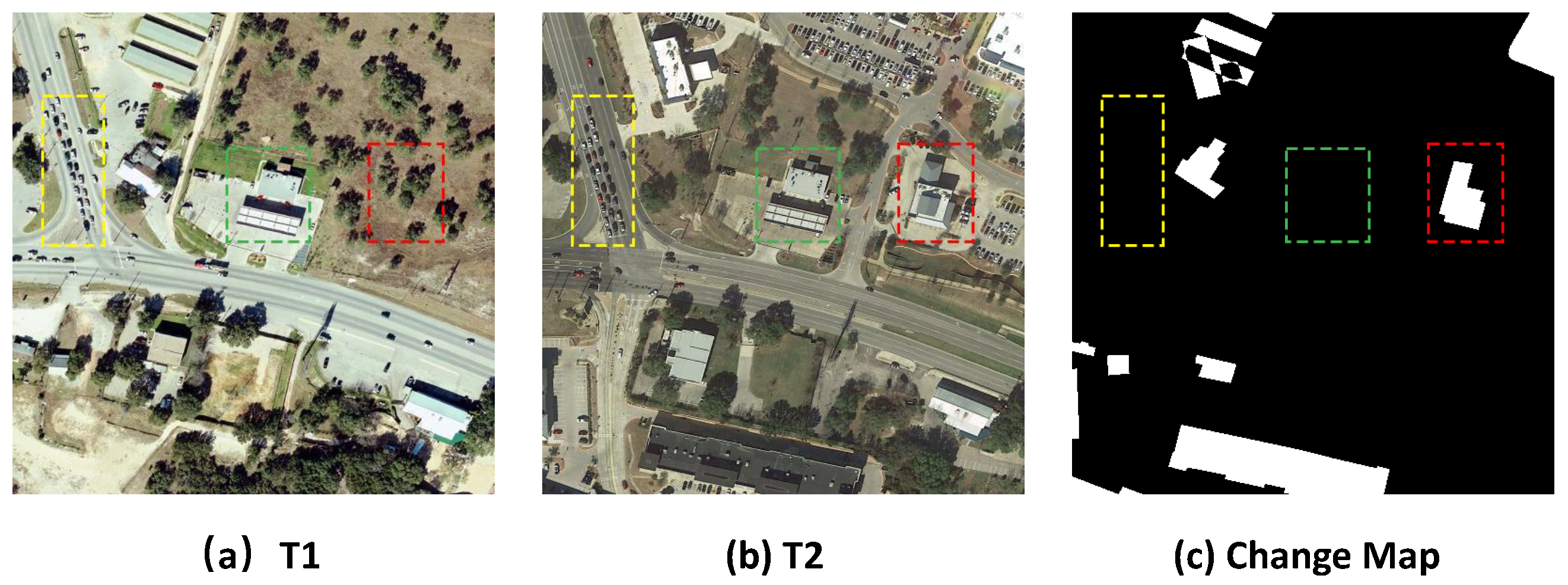
CD faces a series of challenges, as shown in Figure 1. The core task of CD is to track the changes that users want to highlight, such as new buildings (red box), while ignoring changes caused by external factors (green box), such as environmental changes, lighting conditions, fog, or seasonal variations. It also involves filtering out uninteresting targets, such as traffic flow (yellow box). The difficulty of the task lies in the fact that the same feature target presents different spectral features at different time points as well as spatial locations due to environmental factors such as lighting conditions, shooting angle, and atmospheric conditions. Therefore, an excellent CD needs to identify and localize the feature target of interest, and at the same time be able to distinguish between real changes and pseudo-changes caused by environmental noise, which requires powerful feature extraction, spatial–temporal modeling, and change discrimination capabilities. The combination of these capabilities enables the model to accurately capture changes at points of interest in complex scenes and ensure reliable CD results.
By rethinking the task of CD in remote sensing imagery, we find that it is closely related to the remote sensing image semantic segmentation task. This is because in essence, the CD task can be viewed as an intensive change pixel segmentation task. The difference is that this task requires remote sensing images that have been bi-temporal and co-registered as two inputs X 1 , X 2 to the model. In this case, the determination of positive and negative samples is based on whether they have different semantics within different temporal phases at the same geographic location. This means assessing whether the change map label Y corresponds with the model output. Under the optimization objective of minimizing the empirical loss, these two tasks can be formulated as m i n L ( F θ ( X ) , Y ) and m i n L ( F θ ( X 1 , X 2 ) , Y ) . However, the temporal information between bi-temporal phases is wasted if CD is only used as an ordinary semantic segmentation task, so the interactive fusion between bi-temporal feature information also needs to be considered by the model F θ .
Traditional CD methods heavily rely on the results of difference maps. If a significant amount of information is lost during the generation of difference maps, it can lead to unstable accuracy in detection results. Deep learning has been proven to be an effective means of feature learning, capable of automatically extracting abstract features of complex objects in a multi-level manner. The end-to-end structure of deep learning enables us to directly obtain CD results from multi-temporal remote sensing images. We summarize the processing workflow of the CD task into three stages: (1) extraction of bi-temporal features, (2) interaction and fusion of bi-temporal features, (3) discriminative feature generation for the final change map. With the continuous development of high-resolution remote sensing, both ConvNet-based [8,9,10,11] and Transformer-based [12,13,14] methods, driven by a large amount of remote sensing data [8,9,15,16,17,18,19], have shown excellent performance.
Most approaches consider the CD task as a task of dense pixel segmentation [20,21,22], which aligns with the view that these tasks are closely related to semantic segmentation tasks. Therefore, these methods attempt to obtain a larger receptive field in the bi-temporal feature extraction stage. Methods based on ConvNet, limited by the receptive field of convolutional kernels, often seek to expand the receptive field as much as possible through mechanisms such as dilated convolution [23], channel attention [24], spatial attention [25], and mixed attention of channel and spatial [26]. Methods based on Transformer use self-attention with a full receptive field to capture global relationships in spatial–temporal features. However, traditional self-attention is still hindered by quadratic computational complexity with respect to the number of pixels. Therefore, most Transformer-based methods aim to reduce the number of pixels to reduce computational cost.
In the feature interaction and fusion stage, the model integrates the results from the feature extraction part and extracts change information from the bi-temporal data. Therefore, it may be necessary to consider the processing of feature information at multiple stages and scales. During these processes, the model needs to organically fuse features at the same scale from the two temporal phases, which can be achieved through various operations such as subtraction, concatenation, summation, and so on. Effective interaction fusion helps preserve the essential features of land changes and distinguish them from invariant features. Therefore, at this stage, most methods attempt to introduce attention blocks to help the model focus on change-related features. In the final discrimination stage of the change map, there are two approaches. The first is based on pixel classification, which is similar to how semantic segmentation tasks are approached. In this method, the processed change features are projected onto a multi-channel classification map to obtain the final classification result for change pixels. The second approach is based on metric learning [27], which posits that changes can be discerned by measuring the distances between features. Consequently, a contrastive loss is employed to increase the distance between feature vectors that represent changing regions during the optimization process, while reducing the distance between feature vectors representing unchanged regions. Ultimately, a simple threshold is used to obtain the final change map, such as [8,9].
It is well-known that CNNs enhance the translational invariance and local inductive bias of the network through locally shared convolutional kernels, while Transformer is initialized with dot product self-attention which is by definition a global one-dimensional operation, resulting in the same weight of attention assigned to all pixel features, which implies that some of the inductive biases in the Transformer-based model have to be learned either through a large amount of data or by introducing effective task experience [28]. Therefore, we try to summarize some inductive biases for the CD task and introduce them into our model, and design a new encoder as well as a feature interaction fusion module to achieve better CD results in remote sensing images. On the one hand, the CD task, as an intensive segmentation task, requires both a global receptive field for the change classification task and local information for accurate edge segmentation of the change graph. Therefore, in the extraction stage of bi-temporal features, we would like to obtain a global receptive field that approximates self-attention without incurring such an expensive cost as on the self-attention side. At the same time, localization is introduced in the change information interaction fusion stage to accomplish better change map segmentation. On the other hand, the CD task needs to consider how to capture and establish the correlation between bi-temporal co-registered images on top of the dense segmentation task. However, most methods rely only on simple operations such as differencing and splicing between bi-temporal features to integrate the bi-temporal features, and this direct feature fusion strategy makes it difficult to extract change feature information effectively.
Our study aims to optimize the remote sensing image CD process by exploring the essentials of the CD task by introducing certain inductive biases, especially in Transformer-based models. The CD task requires the model to be able to capture global contextual information, but also needs to preserve local detailed features. We would like to pursue balancing the global perceptual field with the local information to improve the global contextual perceptual field while reducing the computational complexity, so as to capture the temporal change features of feature targets more efficiently. We introduce a simple, flexible, and powerful dilated neighborhood attention module (DiNA) into the whole process of CD. Based on DiNA, we constructed DiNAT for embedding into the Transformer structure. By stacking DiNAT modules with different expansion rates, we construct an encoder structure for temporal feature extraction, which allows the sense field to grow exponentially in the feature extraction phase and captures the context at a farther range without any additional computational cost, and augment the change feature while filtering the pseudo-change noise in the interaction phase of the bi-temporal change features by acquiring the inductive bias of the local neighborhoods by means of it, further capturing the temporal-phase semantic change features of the CD task. In addition, we improved DINA and obtained Cross-NA, and constructed the Temporal Neighborhood Cross Differ Module based on Cross-NA to improve the interaction of temporal information to help the model better capture the change information between bi-temporal features, thus obtaining better results.
The contributions of our work can be summarized as follows:
  • We proposed a Transformer-based Siamese network structure called BTNIFormer for addressing CD tasks in remote sensing images. By considering the key aspects of CD from the perspective of semantic segmentation, we employ a sparse sliding-window attention mechanism named DiNA that localizes the attention scope of each pixel to its nearest neighborhood. This introduces inductive bias into the CD task, leading to improved results.
  • By stacking DiNAT with different dilation rates, we construct an Encoder structure that achieves a global receptive field close to self-attention without incurring quadratic computational costs.
  • The Temporal Neighborhood Cross Differ Module, which is composed of the Cross-NA module, is used at each scale stage of the bi-temporal feature map to realize more effective extraction of spatial–temporal variation information and filtering of variation noise.
  • We conducted extensive experiments on two publicly available CD datasets to validate the effectiveness of our approach. Through quantitative and qualitative experimental analysis, our network demonstrated fewer misclassifications and more precise change result edge segmentation effects.
The remaining sections of this paper are organized as follows. The related work is introduced in Section 2. Section 3 provides the conceptual background and implementation details of our proposed method. Experimental results are presented and analyzed in Section 4. The conclusion and future prospects are discussed in Section 5.
2. Related Works

2.1. Recent Binary CD Works

In recent years, most of the work in CD has focused on improving and optimizing the CD processing pipeline we outlined. FC-EF, FC-Siam-Conc, and FC-Siam-Diff [10] are three networks designed based on Fully Convolutional Neural Networks (FCNNs) [29], differing in the choice of when to fuse features and the manner of fusion interaction. DTCDSCN [11] introduces channel attention and spatial attention to construct a dual attention module to enhance feature discrimination. STANet [9] is a metric learning-based method that captures spatial–temporal dependencies at different scales using block-wise self-attention. Bit [30] combines Convolutional Neural Networks (CNNs) with Transformers, mapping bi-temporal features extracted by CNN into dense high-level semantic tokens and enhancing these temporal features using self-attention. ChangFormer [14] fine-tunes the network structure of SegFormer [31] and reduces the pixel count in feature maps using spatial reduction attention (SRA) [32] to alleviate computational costs. Despite achieving outstanding performance in CD, ConvNet-based methods still lack the ability to effectively capture long-range spatial–temporal information. Meanwhile, self-attention mechanisms come with higher computational costs, demanding greater computational resources and time. Therefore, improving CD methods remains an important research direction. In this paper, we propose a Transformer-based CD method that combines the strengths of both approaches to address these challenges.

2.2. Sparse Attention in Transformer

Scaled dot product attention [33] is defined as an operation on a query and a set of key–value pairs. In self-attention, Q, K, and V originate from different projections of the same input. The dot product of the query and key values is computed and scaled, the attentional weights are normalized by softmax, and finally the values are weighted according to the weights. It can be expressed as follows:
A t t e n t i o n ( Q , K , V ) = s o f t m a x Q K T d V
where d is the embedding dimension. In Transformers, it is also common to use multi-head attention, which splits Q , K , V into multiple groups and performs dot product operations in parallel, with the expectation that each head learns features from a different perspective separately.
In the standard self-attention mechanism, each token needs to pay attention to all other tokens. The key advantage of the self-attention mechanism is that it is able to capture the dependencies between different positions in the input sequence without being limited by a fixed sliding window or convolutional kernel size. This makes it perform well in processing sequence data, and it is widely used in deep learning tasks in natural language processing and other areas [34]. However, if given an input X R n × d , n is the number of tokens and d is the embedding dimension. This operation has a complexity of O ( n 2 d ) and a space complexity O ( n 2 d ) for the attention weights. Especially in vision, most operations process two-dimensional image pixels one-dimensionally after additional position coding, which is unacceptably expensive to process.
Sparsification is an effective practice and it has been observed that the attention matrix learned by Transformer is usually very sparse at most data points [35]. Therefore, we can try to reduce the computational complexity by introducing structural bias to limit the number of query–key pairs that each query is concerned with. The limitation of attentional scope was mentioned by Vaswani et al. [33] in the development of the Transformer. Child et al. [35] proposed the Sparse Transformer, which utilizes the sparse kernel attention mechanism in addition to extending to deeper variants. With this approach, the model can be trained more efficiently on longer data sequences. There have been other works on sparse attention, such as Longformer [36], Routing Transformer [37], CcNet [38], and Bigbird [39], and in Figure 2, we visualize the original self-attention as well as the attention weight matrices for several sparse attentions. All these works share a common feature: reducing the cost of self-attention in the inevitable case of longer token sequences, but still maintaining the global context.

2.3. Vision in Transformer

Dosovitskiy et al. [40] proposed a Transformer-based image classifier that merely consists of a Transformer encoder and an image tokenizer, named Vision Transformer (ViT). Previous works, such as DETR [41], explored CNN–Transformer hybrids for object detection, and ViT formalizes the application of pure Transformer structures in the field of computer vision. Vit divides the input image into non-overlapping patches by non-overlapping convolution and tokenizes each patch to be fed into the Transformer for subsequent processing, thus enabling the direct application of the standard Transformer to the image. Content-dependent long-range interaction ability has enabled successful application of ViTs and their variations for various computer vision tasks, such as classification, detection, and segmentation. Following the success of ViTs in computer vision, there has been a significant increase in the use of Transformer-based frameworks in the remote sensing community [42]. These are utilized in many tasks, including very high-resolution image classification [43], change detection [44], pan sharpening [45], and building detection [46].
Notably, ViT approaches or beats the state of the art on several vision benchmarks when pre-trained on the large public ImageNet-21k dataset or the private JFT-300M dataset. However, due to its lack of some of the generalization biases inherent to CNNs, such as translational isovariance and localization, it is no longer competitive when trained on small to medium-sized datasets. At the same time, the memory computation consumption with token length squared level increase makes it not very suitable for semantic segmentation, which requires fine details such as contours most of the time, especially in the early stage of computer vision modeling. With further research, Transformer has proposed different architectures for various computer vision tasks including image classification and image segmentation such as ViT, Segmentation Transformer (SETR) [47], Pyramid Vision Transformer (PVT) [32], Visual Transformer using Shift Window (SwinTransformer) [48], and SegFormer [31]. These Transformer networks have relatively larger effective receptive fields (ERFs) [49] compared to deep ConvNets, providing greater contextual modeling capabilities between any pair of pixels in an image than ConvNets.

3. Materials and Methods

3.1. Overall Architecture

Figure 3 shows the overall architecture of our method. It consists of Siamese Neighborhood Transformer Encoder with shared weights in parallel composed of DiNAT blocks, shown in Figure 3b, Temporal Neighborhood Cross Differ Module for bi-temporal change information interaction, and a Simple Multi-Scale Aggregation Change Decoder for aggregating and discriminatively generating change results. So, our pipeline can be briefly described as the proposed BTNIFormer taking the registered bi-temporal remote sensing images as input. However, the Siamese Neighborhood Transformer Encoder consists of DiNAT blocks to obtain the feature maps on four different scales, after which the hierarchical pairs of bi-temporal features are passed through the Temporal Neighborhood Cross Differ module for temporal information interaction and extraction to enhance the change feature. Finally, all the change features on the scale are aggregated and discriminated by Simple Multi-Scale Aggregation Change Decoder to generate the final binary change map. At the same time, inspired by Zheng et al.’s work [50], in most cases we are not able to cognize the process of feature target change through the bi-temporal image alone, so we can assume that the bi-temporal image has a temporal symmetry that is anisotropic for the CD task of bi-temporal detection, which is formulated as Y t 1 > t 2 = Y t 2 > t 1 . Intuitively, if we exchange the inputs of the bi-temporal detection, it does not have any impact on the CD output in any way. We introduce the inductive biases of an undirected nature by maintaining the symmetry of the bi-temporal feature processing flow when constructing the network structure.
Since feature targets in remote sensing images are characterized by their multi-scale nature, our encoder computation has four stages with different spatial resolutions, illustrated in Figure 3a. In each stage, features are first spatially downsampled by a convolutional layer, and then feature extraction is performed by overlapping DiNAT blocks with different dilations while obtaining a wider sensing field, and finally feature maps with different scale resolutions of the four stages are generated. How to effectively capture target semantic changes in complex feature scenes is one of the main challenges of the CD task. Therefore, we use Temporal Neighborhood Cross Differ Module, as shown in Figure 3c, to interact and fuse the temporal features of the bi-temporal feature maps on the current scale, to enhance the changing features of each phase while filtering irrelevant noise. After that, we concat the enhanced bi-temporal features in the channel dimension and compress the channel by convolutional layer. In recent years, many models have been investigating how to design a better decoder (the feature extraction is usually carried out by a pre-trained backbone), shown in Figure 3d, resulting in a decoder that is heavier and more complex, but our structure has already gained a sufficiently large receptive field in feature extraction and established the interaction and connection of the change information features between the bi-temporal phases. Therefore, in the final stage, we only need a simple multi-scale aggregated change decoder with a simple structure to generate the binary change mask.

3.2. Dilated Neighborhood Attention

The most straightforward way to limit the range of self-attention is to make each pixel focus only on pixels within its neighborhood, which produces a dynamic window of attention similar to a convolutional window, thus introducing local inductive biases. Although such nonlocal and sparse restrictions on self-attention have been shown to be promising, they have not been well-studied in the context of hierarchical visual transformations. The introduction of Window Self-Attention (WSA) in SwinTransformer [48] restricts the scope of self-attention operations to the window and is cleverly and efficiently implemented with the help of the Cyclic Shift operation. To extend the local receptive field and reintroduce global context into the hierarchical vision Transformer, we introduce Dilated Neighborhood Attention (DiNA), which spans the neighborhood over a wider range by increasing the dilated value while maintaining the overall attentional span. DiNA can be used as a global operation of sparsity. DiNA restricts self-attention through a sliding window and achieves a similarity to convolution and dilation convolution by varying dilation rate restrictions on fully connected layers. These restrictions reduce the computational burden and introduce useful inductive biases.
Given input X R n × d , whose rows are d-dimensional token vectors, and query and key linear projections of X, Q, and K, and relative positional biases between any two tokens i and j, B i , j , we define neighborhood attention weights for the ith token with neighborhood size k. Token i’s jth nearest neighbors are denoted as ρ j r ( i ) . A i k is the matrix multiplication of the ith token’s query projection, and its k nearest neighboring tokens’ key projections. We can then define r-dilated neighborhood attention weights for the ith token with neighborhood size k, A i k , r , as follows:
A i ( k , r ) = Q i K ρ 1 T ( i ) T + B i , ρ 1 r ( i ) Q i K ρ 2 T ( i ) T + B i , ρ 2 δ ( i ) Q i K ρ k T ( i ) T + B i , ρ k r ( i )
We define r-dilated neighboring values for the ith token with neighborhood size k, V i k , r :
V i ( k , r ) = V ρ 1 r ( i ) T V ρ 2 r ( i ) T V ρ k r ( i ) T T
DiNA output for the ith token with neighborhood size k is then defined as follows:
DiNA k r ( i ) = s o f t m a x A i ( k , r ) d k V i ( k , r )
where d is the scaling parameter, and d is the embedding dimension.
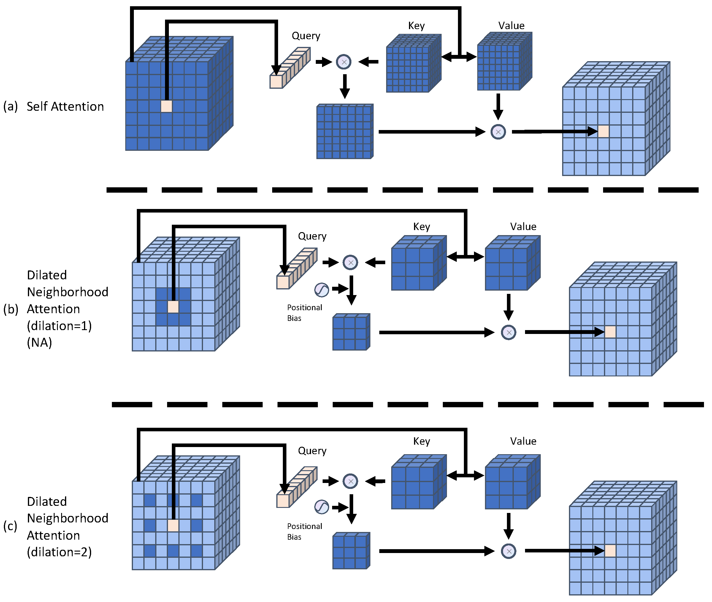
This operation is repeated for every pixel in the feature map. Illustrations of this operation are presented in Figure 4. From the definition above, it is evident that as k increases, A i k approaches the self-attention weights, and V i k approaches V i itself, resulting in neighborhood attention approaching self-attention. However, when dilation is set to 1, DiNA degenerates to NA, meaning that the query values are limited to the neighborhood with a relationship similar to that between convolution and dilation convolution.
We compare the computational cost of different variants of the self-attention mechanism in Table 1, and DiNA maintains the contextual symmetry with WSA with the same computational cost as well as memory footprint. Since Swin’s feature map is divided into non-overlapping windows, pixels within the same window will only pay attention to each other, and although it interacts with the information by offsetting the window, it does not give its positional information, making the edge pixels acquire an asymmetric context around them.
In order to introduce the DiNA mechanism into our CD detection structure, as shown in Figure 3b, we built the Dilated Neighborhood Attention Transformer (DiNAT) block by referring to the encoder structure of Transformer. Similarly, the Neighborhood Attention Transformer (NAT) block is constructed when the dilated value is set to 1.

3.3. Siamese Dilated Neighborhood Transformer Encoder

To achieve a sizeable receptive field while circumventing the Gridding Effect, we fabricated the Siamese Neighborhood Transformer Encoder through the incorporation of DiNAT blocks with varying dilation rate. We compare FLOPs, memory usage, and receptive field sizes under different attentional modes of stacking in Table 2. We calculate receptive field size with respect to the number of layers, , kernel size k, and number of tokens n, which is equal to the size of the input picture. Window Self-Attention alone would suffer from a fixed-value receptive field, but the pixel shift in SWSA expands the receptive field linearly. Stacking the DiNAT block with different dilation rates can expand receptive fields exponentially. Self-attention has the maximum global receptive field, which comes at the expense of a quadratic computational cost.
We configured the encoder’s structure with reference to the success of previous CNN structures (ResNet [51]) with ViT-based approaches (PVT [32], Swin-Transformer [48], and SegFormer [31]). Figure 3a shows a schematic of the entire encoder network architecture. The Siamese Dilated Neighborhood Transformer Encoder comprises four stages, each representing different resolution scales. In the first stage, the input is embedded through two consecutive 3 × 3 convolutions using 2 × 2 steps, thereby reducing the space size to 1/4 of the input size, albeit with overlapping convolutions rather than non-overlapping convolutions to introduce a useful inductive bias. In the later stages, our method employs overlapping convolutions featuring kernel sizes of 3 × 3 and 2 × 2 stride. This results in a halving of the spatial resolution with a doubling of the number of channels, finally generating four feature maps of scale resolution with sizes indicated by h 4 × w 4 , h 8 × w 8 , h 16 × w 16 , and h 32 × w 32 . The downsampled inputs are entered into DiNA blocks of varying dilation layers at each stage (the number of layers in each phase is three, four, six, and five, respectively). For images’ resolution limit, determined by the maximum size at each scale, we set the highest dilation values to 8, 4, 2, and 1 and interleaved with the NAT module, while the dilation value of the DiNAT module was incremented gradually from 1 to the maximum dilation value.
Specifically, if we are given a pair of bi-temporal CD task image pairs F p r e i , F p o s t i of resolution H × W × 3 , the encoder outputs a feature map F i with a resolution H 2 i + 1 × W 2 i + 1 × C i , where i = 1, 2, 3, 4 and C i + 1 > C i , which will be further processed through the interactive fusion module in the next step.

3.4. Temporal Neighborhood Cross Differ Module

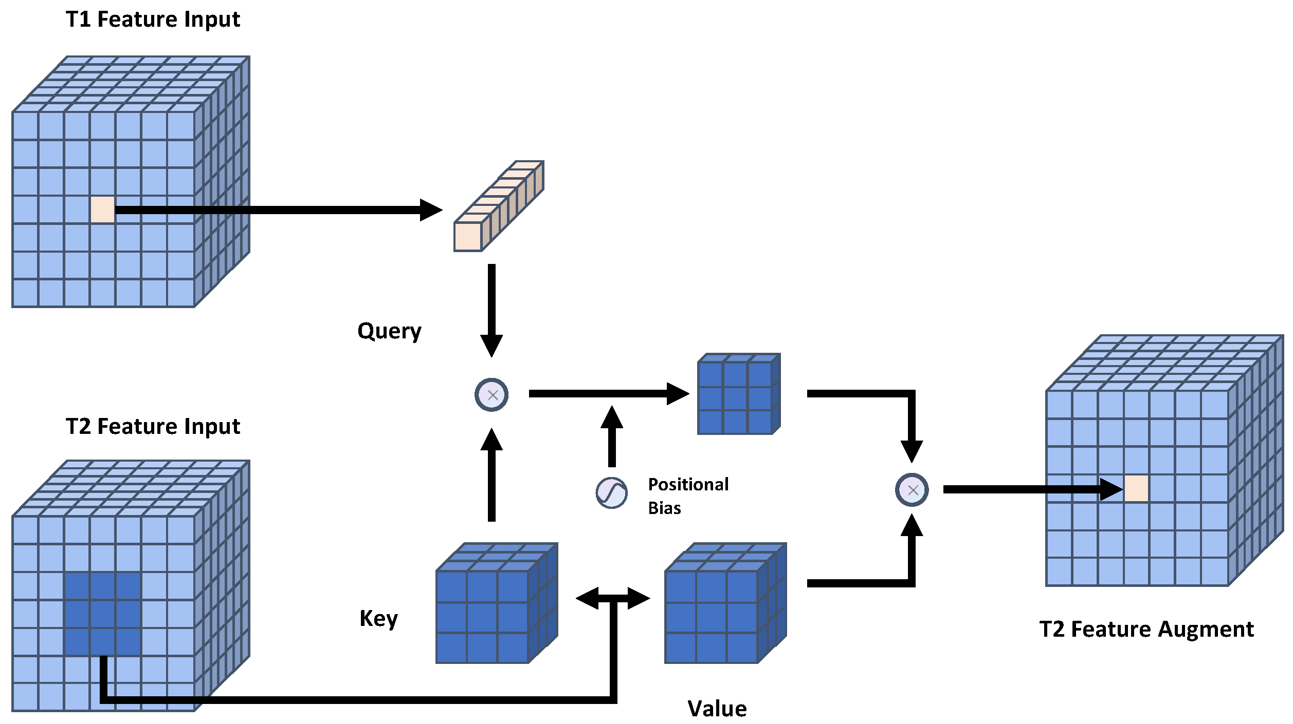
As stated in the motivation section, it is believed that the key element of the CD task is the interaction of bi-temporal features. To address this, the DiNA is introduced into the feature interaction phase. We have constructed a Temporary Neighborhood Cross Differ Module for dual temporal feature interaction using the Cross-NA, which is the variant of DiNA, as the core. Unlike the configuration method used in the encoder phase, the Cross-NA module is utilized for bi-temporal feature interaction at each scale in this phase, with the structure shown in Figure 3c. The Cross-NA is a modified version of the DiNA. We set the expansion rate of DiNA to 1 in this variation. Moreover, as shown in Figure 5, Cross-NA extracts the query from one temporal phase feature and the key and value from another temporal phase feature. The present temporal phase feature improves each phase by computing a correlation score in a k-neighborhood of the prior position at the other temporal phase while eliminating extraneous noise. The interaction process of Temporal Neighborhood Cross Differ Module in the bi-temporal phase can be formulated as follows:
F ˜ p r e i = C r o s s N A k F p o s t i , F p r e i = s o f t m a x A i ( k , 1 ) d k V i ( k , 1 ) + F p r e i , i F ˜ p o s t i = C r o s s N A k F p r e i , F p o s t i = s o f t m a x A i ( k , 1 ) d k V i ( k , 1 ) + F p o s t i , i
After the bi-temporal features are interactively augmented with the other temporal phase separately, we concat them and then fuse them via a convolutional layer. The calculation process is formulated as follows:
F d i f f i = B N R e L U C o n v C a t ( F ˜ p r e i , F ˜ p o s t i ) , i

3.5. Simple Multi-Scale Aggregation Change Decoder

In the decoder stage, we perform channel unification as well as splicing of the multi-scale variation features obtained in the previous stage. The feature map is then resized to its initial dimensions via two gradual upsampling layers. Finally, a convolutional layer is applied to generate the ultimate change map, which can be formulated as follows:
F i = U p s a m p l e ( H 4 , W 4 ) ( L i n e a r ( C i , C ) ( F d i f f i ) ) , i F c h a n g e = L i n e a r ( 4 C , C ) C o n c a t ( F i ) , i M c h a n g e = C o n v U p s a m p l e ( F c h a n g e )

4. Experiments

4.1. Datasets

We conducted experiments on two publicly available CD remote sensing image datasets with three RGB bands: WHU-CD dataset and LEVIR-CD dataset.
WHU-CD [16] contains two aerial high-resolution (0.3 m) images, which were acquired in 2012 and 2016. Since it covers an area that was hit by a 6.3 magnitude earthquake in February 2011 and rebuilt in the following years, there are a large number of building changes in this area, and the size of study image is 32,507 × 15,354. Since no specific segmentation scheme was mentioned in the dataset, we cropped the image into non-overlapping patches with a resolution of 256 × 256 . After that, a random partitioning of the dataset was performed, obtaining 5947 / 743 / 744 pairs for train/validation/test, respectively.
LEVIR-CD [9] is a publicly available large-scale building dataset, containing images from 20 different areas in various cities in Texas, USA. The dataset comprises 637 pairs of high-resolution (0.5 m) remote sensing images of size 1024 × 1024. The building types represented include a range of variants, such as detached houses, tower blocks, small sheds, and large storage facilities. We follow its default dataset split. Due to the limitation of GPU memory capacity, we cut images into small patches of size 256 × 256 with no overlap. Therefore, we obtained 7120 / 1024 / 2048 pairs of patches for training/validation/test, respectively.

4.2. Evaluation Metrics

We evaluate the performance of the proposed method using five confusion matrix-based evaluation metrics, which include overall accuracy (OA), precision (Pre), recall (Rec), F1-score (F1), and Intersection over Union (IoU). Since CD tasks are often accompanied by uneven distribution of sample categories, all metrics represent the evaluation results of change categories. The formulas for these metrics are as follows:
Pre = TP / ( TP + FP ) Rec = TP / ( TP + FN ) OA = ( TP + TN ) / ( TP + TN + FN + FP ) IoU = TP / ( TP + FN + FP ) F 1 = 2 Rec 1 + Pre 1
where TP, FP, TN, and FN refer to true positives, false positives, true negatives, and false negatives, respectively.

4.3. State-of-the-Art Comparison

We have selected several state-of-the-art CD methods that use the attention mechanism for comparison purposes.
STANet [9] is a spatial–temporal attention concatenated neural network that employs metric learning. The network uses ResNet as a base model for feature extraction, with weight-sharing capabilities. The model also incorporates a multi-scale CD self-attention module to effectively model spatial–temporal relations.
DTCDSCN [11] is a multitasking model which performs both CD and semantic segmentation. It introduces channel and spatial attention to exploit interdependencies between channels and spatial locations for improved feature representation.
BiT [30] is a hybrid model of CNN and Transformer. It uses ResNet convolutional blocks for feature extraction at a shallow level, tokenizes the features at a deeper level, and enhances the contextual information of ConvNet features with semantic tokens for modeling in spatial–temporal information.
ChangeFormer [14] is a Transformer-based Siamese network and combines a hierarchically structured Transformer encoder with Multi-Layer Perception (MLP) decoder in a Siamese network architecture to efficiently render the multi-scale long-range details required for accurate CD.

4.4. Implementation Details

Our models are implemented on PyTorch, and the DiNA module was efficiently implemented using the open-source extension of Pyrorch—Natten [52]. All tasks were carried out on a single NVIDIA Tesla V100 GPU. We trained the models using the Binary Cross-Entropy (BCE) Loss and AdamW optimizer, with weight decay set to 0.01 and beta values set to (0.9, 0.999). The learning rate was initially set to 0.0001 and linearly decayed to 0 over the course of 200 epochs. For model training, we set the batch size to 16 due to GPU memory limitations. For data augmentation, we use random crop, flip, Gaussian blur, and random color jittering. In addition, in order to establish the anisotropy of the temporal information between the bi-temporal features, we randomly swap the order of the bi-temporal images.

4.5. Main Results

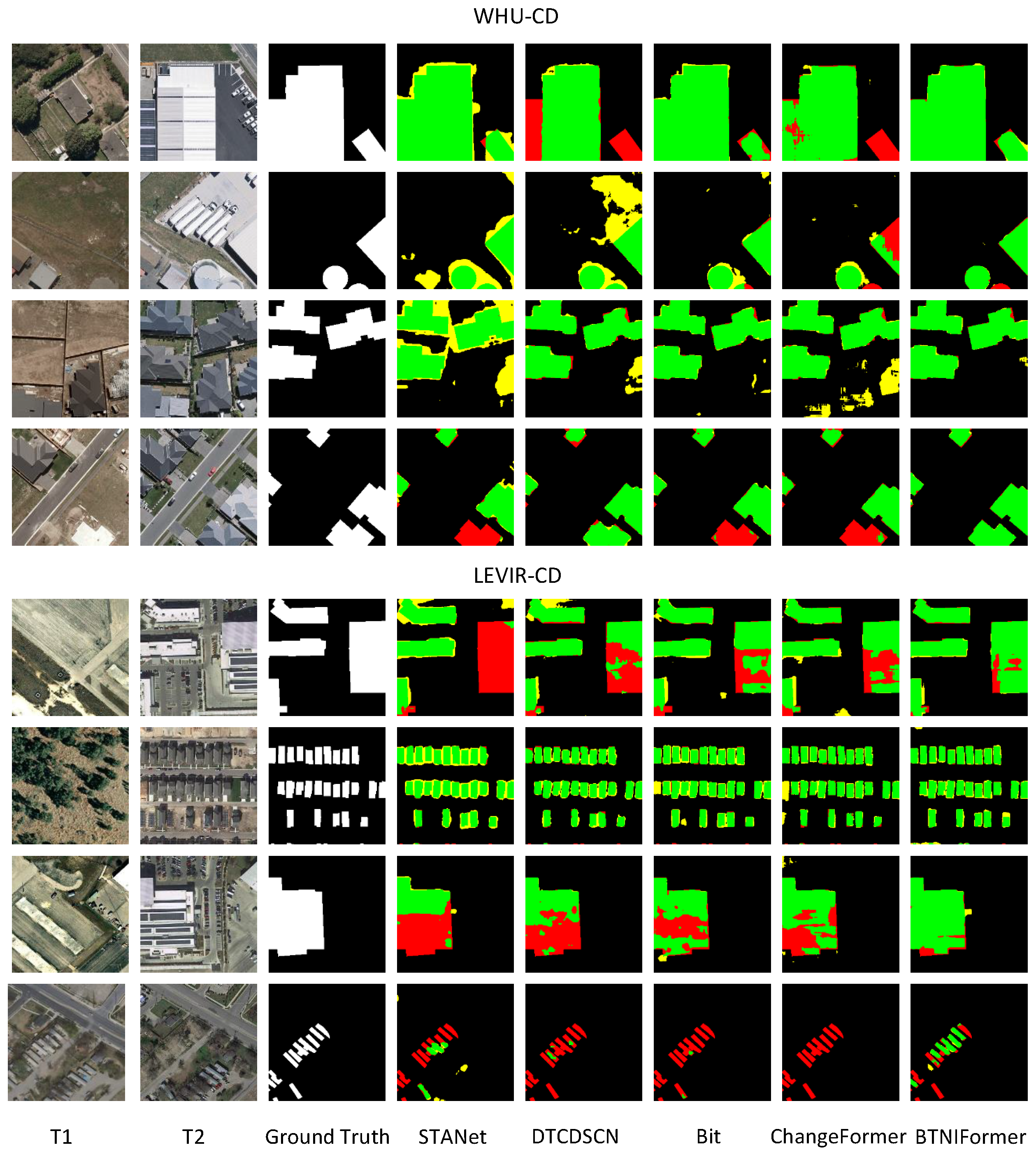
In Table 3, we clearly label and present the overall comparative results of our method and some SOTA methods on the WHU-CD and LEVIR-CD test sets. The results show that our method based on BTNIFormer significantly outperforms other methods on these datasets. Our comparison focuses on ChangeFormer, which is the most competitive in terms of performance and based on the same Transformer architecture. Our model improves WHU-CD and LEVIR-CD by 0.51 / 7.38 / 12.00 % and 0.16 / 1.62 / 2.75 % on OA/F1/IoU, respectively. We qualitatively compare the performance of some representative CD scene samples in the WHU-CD and LEVIR-CD validation sets with SOTA methods, as visualized in Figure 6. Compared to other methods, our approach provides more accurate and complete edge detection results with fewer false positives (in yellow). In addition, we compare the computational cost of different methods in Table 4. The results show that compared to ChangeFormer, BTNIFormer improves the metrics dramatically while almost halving the number of parameters and memory usage, and is an order of magnitude lower in terms of FLOPs. Although in terms of computational cost our method though does not have an advantage over Bit with Resnet as the backbone network, our method improves WHU-CD and LEVIR-CD by 0.6 / 8.77 / 14.09 % and 0.28 / 2.71 / 4.55 % on OA/F1/IoU, which still demonstrates the great advantage of our method. These quantitative and qualitative experimental results show that our method achieves superior performance compared to existing SOTA methods.

4.6. Ablation Studies

To investigate the effectiveness of our method, we conducted exhaustive experiments on different aspects of the model structure using the LEVIR-CD dataset. For ablation experiments, we remove the Cross-NA in the Temporal Neighborhood Cross Differ Module as the baseline, which means that the bi-temporal features are only interacting through concat and convolution operations in this time. Unless stated otherwise, we set embedding dim to 64 and configured the remaining structures.
Encoder selection under the same parameter scale. Most recent models have opted to utilize pre-trained models for feature extraction, which has been proven to be an effective approach based on the results. To validate the performance of our designed encoder, we attempted to replace the feature extraction module with pre-trained ResNet-34 [51] and MiT-b2 [31] structures of the same parameter scale. According to Table 5, our Siamese Dilated Neighborhood Trasnformer Encoder improves the F1 and IoU of ResNet-34 based on convolutional composition by 1.13 % / 1.9 % , while the number of parameters decreases. Compared with the MiT-b2 based on the Transformer structure, our model reduces the number of parameters by about 20 % while still improving the F1 and IoU by 0.05 % / 0.09 % . Thus, our feature extraction module outperformed the other architectures.
Which layers need to interact with temporal information? We try to perform feature interaction layer ablation at each of the four stages of feature extraction. As shown in Table 6, the best detection results can be obtained by performing feature interaction at all stages. Additionally, we noted a positive correlation between the accuracy of the model and the quantity of interacting layers. We believe that interaction at all stages is more helpful for the extraction of multi-scale variation features, as it does not intervene in the subsequent process of feature extraction.
The interaction mode of temporal information. To explore how to interact during the feature interaction phase, we compared different attentional modes during the interaction phase. As shown in Table 7, the NA we chose achieved the best performance. Using NA for interaction at this stage shows an improvement of 0.19/0.07% and 0.34/0.13% in terms of F1 and IoU compared to Self-attention and DiNA. We argue that the introduction of local inductive bias at the interaction stage is effective because the time-varying features at the interaction stage only need to query the semantics of the pixels in the neighborhood, and do not need to be used in the same way as the feature extraction phase to use DiNA or self-attention to obtain a larger perceptual field. On the other hand, the comparison between DiNA and SA again proves that the sparsification approach has better results.

5. Conclusions

In this paper, we propose a Transformer-based Siamese architecture called BTNIFormer for remote sensing change detection (CD). BTNIFormer introduces Dilated Neighborhood Attention (DiNA), which effectively locates the autonomous attention of each pixel to the neighborhood, thus achieving effective capture of spatial–temporal change features by the model. We further design a Temporal Neighborhood Cross Differ Module for the interaction of dual temporal feature information, which enhances the changing features while suppressing noise changes. We validated our method by conducting extensive experiments on two publicly available CD datasets. Our extensive qualitative and quantitative results reveal the benefits of the proposed contributions. The proposed method achieves SOTA performance on all datasets, with significant computational advantages compared to recent Transformer-based methods. These results demonstrate the enormous advantages and potential of the sparse attention mechanism in the field of remote sensing image change detection. We hope that these works can contribute to the further research of Transformer in this field in the future.

Author Contributions

Conceptualization, H.M. and R.N.; methodology, H.M.; software, H.M. and B.L.; validation, H.M. and Y.W.; formal analysis, H.M. and L.Z.; investigation, H.M.; resources, H.M.; data curation, H.M. and L.Z.; writing—original draft preparation, H.M.; writing—review and editing, R.N.; visualization, H.M.; supervision, R.N.; project administration, H.M. All authors have read and agreed to the published version of the manuscript.

Funding

This research received no external funding.

Data Availability Statement

The data presented in this study are available from the author upon reasonable request.

Conflicts of Interest

The authors declare no conflict of interest.

References

  1. Singh, A. Review Article Digital change detection techniques using remotely-sensed data. Int. J. Remote Sens. 1989, 10, 989–1003. [Google Scholar] [CrossRef]
  2. De Bem, P.P.; de Carvalho Junior, O.A.; Fontes Guimarães, R.; Trancoso Gomes, R.A. Change detection of deforestation in the Brazilian Amazon using landsat data and convolutional neural networks. Remote Sens. 2020, 12, 901. [Google Scholar] [CrossRef]
  3. Wen, D.; Huang, X.; Bovolo, F.; Li, J.; Ke, X.; Zhang, A.; Benediktsson, J.A. Change detection from very-high-spatial-resolution optical remote sensing images: Methods, applications, and future directions. IEEE Geosci. Remote Sens. Mag. 2021, 9, 68–101. [Google Scholar] [CrossRef]
  4. Kumar, S.; Jain, K. A multi-temporal Landsat data analysis for land-use/land-cover change in Haridwar Region using remote sensing techniques. Procedia Comput. Sci. 2020, 171, 1184–1193. [Google Scholar] [CrossRef]
  5. Lu, Y.; Wu, P.; Ma, X.; Li, X. Detection and prediction of land use/land cover change using spatiotemporal data fusion and the Cellular Automata–Markov model. Environ. Monit. Assess. 2019, 191, 68. [Google Scholar] [CrossRef]
  6. Gupta, R.; Hosfelt, R.; Sajeev, S.; Patel, N.; Goodman, B.; Doshi, J.; Heim, E.; Choset, H.; Gaston, M. xbd: A dataset for assessing building damage from satellite imagery. arXiv 2019, arXiv:1911.09296. [Google Scholar]
  7. Kucharczyk, M.; Hugenholtz, C.H. Remote sensing of natural hazard-related disasters with small drones: Global trends, biases, and research opportunities. Remote Sens. Environ. 2021, 264, 112577. [Google Scholar] [CrossRef]
  8. Shi, Q.; Liu, M.; Li, S.; Liu, X.; Wang, F.; Zhang, L. A deeply supervised attention metric-based network and an open aerial image dataset for remote sensing change detection. IEEE Trans. Geosci. Remote Sens. 2021, 60, 5604816. [Google Scholar] [CrossRef]
  9. Chen, H.; Shi, Z. A spatial-temporal attention-based method and a new dataset for remote sensing image change detection. Remote Sens. 2020, 12, 1662. [Google Scholar] [CrossRef]
  10. Daudt, R.C.; Le Saux, B.; Boulch, A. Fully convolutional siamese networks for change detection. In Proceedings of the 2018 25th IEEE International Conference on Image Processing (ICIP), Athens, Greece, 7–10 October 2018; pp. 4063–4067. [Google Scholar] [CrossRef]
  11. Liu, Y.; Pang, C.; Zhan, Z.; Zhang, X.; Yang, X. Building change detection for remote sensing images using a dual-task constrained deep siamese convolutional network model. IEEE Geosci. Remote Sens. Lett. 2020, 18, 811–815. [Google Scholar] [CrossRef]
  12. Li, Q.; Zhong, R.; Du, X.; Du, Y. TransUNetCD: A hybrid transformer network for change detection in optical remote-sensing images. IEEE Trans. Geosci. Remote Sens. 2022, 60, 5622519. [Google Scholar] [CrossRef]
  13. Zhang, C.; Wang, L.; Cheng, S.; Li, Y. SwinSUNet: Pure transformer network for remote sensing image change detection. IEEE Trans. Geosci. Remote Sens. 2022, 60, 5224713. [Google Scholar] [CrossRef]
  14. Bandara, W.G.C.; Patel, V.M. A transformer-based siamese network for change detection. In Proceedings of the IGARSS 2022-2022 IEEE International Geoscience and Remote Sensing Symposium, Kuala Lumpur, Malaysia, 17–22 July 2022; pp. 207–210. [Google Scholar] [CrossRef]
  15. Lebedev, M.; Vizilter, Y.V.; Vygolov, O.; Knyaz, V.A.; Rubis, A.Y. Change detection in remote sensing images using conditional adversarial networks. Int. Arch. Photogramm. Remote Sens. Spat. Inf. Sci. 2018, 42, 565–571. [Google Scholar] [CrossRef]
  16. Ji, S.; Wei, S.; Lu, M. Fully convolutional networks for multisource building extraction from an open aerial and satellite imagery data set. IEEE Trans. Geosci. Remote Sens. 2018, 57, 574–586. [Google Scholar] [CrossRef]
  17. Shen, L.; Lu, Y.; Chen, H.; Wei, H.; Xie, D.; Yue, J.; Chen, R.; Lv, S.; Jiang, B. S2Looking: A satellite side-looking dataset for building change detection. Remote Sens. 2021, 13, 5094. [Google Scholar] [CrossRef]
  18. Zhang, C.; Yue, P.; Tapete, D.; Jiang, L.; Shangguan, B.; Huang, L.; Liu, G. A deeply supervised image fusion network for change detection in high resolution bi-temporal remote sensing images. ISPRS J. Photogramm. Remote Sens. 2020, 166, 183–200. [Google Scholar] [CrossRef]
  19. Verma, S.; Panigrahi, A.; Gupta, S. Qfabric: Multi-task change detection dataset. In Proceedings of the IEEE/CVF Conference on Computer Vision and Pattern Recognition, Nashville, TN, USA, 20–25 June 2021; pp. 1052–1061. [Google Scholar]
  20. Fang, S.; Li, K.; Shao, J.; Li, Z. SNUNet-CD: A densely connected Siamese network for change detection of VHR images. IEEE Geosci. Remote Sens. Lett. 2021, 19, 8007805. [Google Scholar] [CrossRef]
  21. Chen, P.; Zhang, B.; Hong, D.; Chen, Z.; Yang, X.; Li, B. FCCDN: Feature constraint network for VHR image change detection. ISPRS J. Photogramm. Remote Sens. 2022, 187, 101–119. [Google Scholar] [CrossRef]
  22. Zheng, Z.; Zhong, Y.; Tian, S.; Ma, A.; Zhang, L. ChangeMask: Deep multi-task encoder-transformer-decoder architecture for semantic change detection. ISPRS J. Photogramm. Remote Sens. 2022, 183, 228–239. [Google Scholar] [CrossRef]
  23. Yu, F.; Koltun, V. Multi-scale context aggregation by dilated convolutions. arXiv 2015, arXiv:1511.07122. [Google Scholar]
  24. Hu, J.; Shen, L.; Sun, G. Squeeze-and-excitation networks. In Proceedings of the IEEE Conference on Computer Vision and Pattern Recognition, Salt Lake City, UT, USA, 18–23 June 2018; pp. 7132–7141. [Google Scholar]
  25. Jaderberg, M.; Simonyan, K.; Zisserman, A. Spatial transformer networks. Adv. Neural Inf. Process. Syst. 2015, 28. [Google Scholar]
  26. Woo, S.; Park, J.; Lee, J.Y.; Kweon, I.S. Cbam: Convolutional block attention module. In Proceedings of the European Conference on Computer Vision (ECCV), Munich, Germany, 8–14 September 2018; pp. 3–19. [Google Scholar]
  27. Kulis, B. Metric learning: A survey. Found. Trends® Mach. Learn. 2013, 5, 287–364. [Google Scholar] [CrossRef]
  28. Xu, Y.; Zhang, Q.; Zhang, J.; Tao, D. Vitae: Vision transformer advanced by exploring intrinsic inductive bias. Adv. Neural Inf. Process. Syst. 2021, 34, 28522–28535. [Google Scholar]
  29. Milletari, F.; Navab, N.; Ahmadi, S.A. V-net: Fully convolutional neural networks for volumetric medical image segmentation. In Proceedings of the 2016 Fourth International Conference on 3D Vision (3DV), Stanford, CA, USA, 25–28 October 2016; pp. 565–571. [Google Scholar] [CrossRef]
  30. Chen, H.; Qi, Z.; Shi, Z. Remote sensing image change detection with transformers. IEEE Trans. Geosci. Remote Sens. 2021, 60, 1–14. [Google Scholar] [CrossRef]
  31. Xie, E.; Wang, W.; Yu, Z.; Anandkumar, A.; Alvarez, J.M.; Luo, P. SegFormer: Simple and efficient design for semantic segmentation with transformers. Adv. Neural Inf. Process. Syst. 2021, 34, 12077–12090. [Google Scholar]
  32. Wang, W.; Xie, E.; Li, X.; Fan, D.P.; Song, K.; Liang, D.; Lu, T.; Luo, P.; Shao, L. Pyramid vision transformer: A versatile backbone for dense prediction without convolutions. In Proceedings of the IEEE/CVF International Conference on Computer Vision, Montreal, BC, Canada, 11–17 October 2021; pp. 568–578. [Google Scholar]
  33. Vaswani, A.; Shazeer, N.; Parmar, N.; Uszkoreit, J.; Jones, L.; Gomez, A.N.; Kaiser, Ł.; Polosukhin, I. Attention is all you need. In Proceedings of the 31st Conference on Neural Information Processing Systems, Long Beach, CA, USA, 4–9 December 2017; pp. 5998–6008. [Google Scholar]
  34. Lin, T.; Wang, Y.; Liu, X.; Qiu, X. A survey of transformers. AI Open 2022, 3, 111–132. [Google Scholar] [CrossRef]
  35. Child, R.; Gray, S.; Radford, A.; Sutskever, I. Generating long sequences with sparse transformers. arXiv 2019, arXiv:1904.10509. [Google Scholar]
  36. Beltagy, I.; Peters, M.E.; Cohan, A. Longformer: The long-document transformer. arXiv 2020, arXiv:2004.05150. [Google Scholar]
  37. Roy, A.; Saffar, M.; Vaswani, A.; Grangier, D. Efficient content-based sparse attention with routing transformers. Trans. Assoc. Comput. Linguist. 2021, 9, 53–68. [Google Scholar] [CrossRef]
  38. Huang, Z.; Wang, X.; Huang, L.; Huang, C.; Wei, Y.; Liu, W. Ccnet: Criss-cross attention for semantic segmentation. In Proceedings of the IEEE/CVF International Conference on Computer Vision, Seoul, Republic of Korea, 27 October–2 November 2019; pp. 603–612. [Google Scholar]
  39. Zaheer, M.; Guruganesh, G.; Dubey, K.A.; Ainslie, J.; Alberti, C.; Ontanon, S.; Pham, P.; Ravula, A.; Wang, Q.; Yang, L.; et al. Big bird: Transformers for longer sequences. Adv. Neural Inf. Process. Syst. 2020, 33, 17283–17297. [Google Scholar]
  40. Dosovitskiy, A.; Beyer, L.; Kolesnikov, A.; Weissenborn, D.; Zhai, X.; Unterthiner, T.; Dehghani, M.; Minderer, M.; Heigold, G.; Gelly, S.; et al. An image is worth 16x16 words: Transformers for image recognition at scale. arXiv 2020, arXiv:2010.11929. [Google Scholar]
  41. Yang, A.; Miech, A.; Sivic, J.; Laptev, I.; Schmid, C. Tubedetr: Spatio-temporal video grounding with transformers. In Proceedings of the IEEE/CVF Conference on Computer Vision and Pattern Recognition, New Orleans, LA, USA, 18–24 June 2022; pp. 16442–16453. [Google Scholar]
  42. Aleissaee, A.A.; Kumar, A.; Anwer, R.M.; Khan, S.; Cholakkal, H.; Xia, G.S.; Khan, F.S. Transformers in remote sensing: A survey. Remote Sens. 2023, 15, 1860. [Google Scholar] [CrossRef]
  43. Zhong, Z.; Li, Y.; Ma, L.; Li, J.; Zheng, W.S. Spectral—Spatial transformer network for hyperspectral image classification: A factorized architecture search framework. IEEE Trans. Geosci. Remote Sens. 2021, 60, 5514715. [Google Scholar] [CrossRef]
  44. Zhang, M.; Liu, Z.; Feng, J.; Liu, L.; Jiao, L. Remote Sensing Image Change Detection Based on Deep Multi-Scale Multi-Attention Siamese Transformer Network. Remote Sens. 2023, 15, 842. [Google Scholar] [CrossRef]
  45. Zhou, H.; Liu, Q.; Wang, Y. Panformer: A transformer based model for pan-sharpening. In Proceedings of the 2022 IEEE International Conference on Multimedia and Expo (ICME), Taipei, Taiwan, 18–22 July 2022; pp. 1–6. [Google Scholar]
  46. Chen, K.; Zou, Z.; Shi, Z. Building extraction from remote sensing images with sparse token transformers. Remote Sens. 2021, 13, 4441. [Google Scholar] [CrossRef]
  47. Zheng, S.; Lu, J.; Zhao, H.; Zhu, X.; Luo, Z.; Wang, Y.; Fu, Y.; Feng, J.; Xiang, T.; Torr, P.H.; et al. Rethinking semantic segmentation from a sequence-to-sequence perspective with transformers. In Proceedings of the IEEE/CVF Conference on Computer Vision and Pattern Recognition, Nashville, TN, USA, 20–25 June 2021; pp. 6881–6890. [Google Scholar]
  48. Liu, Z.; Lin, Y.; Cao, Y.; Hu, H.; Wei, Y.; Zhang, Z.; Lin, S.; Guo, B. Swin transformer: Hierarchical vision transformer using shifted windows. In Proceedings of the IEEE/CVF International Conference on Computer Vision, Montreal, BC, Canada, 11–17 October 2021; pp. 10012–10022. [Google Scholar]
  49. Luo, W.; Li, Y.; Urtasun, R.; Zemel, R. Understanding the Effective Receptive Field in Deep Convolutional Neural Networks. arXiv 2017, arXiv:1701.04128. [Google Scholar]
  50. Zheng, Z.; Ma, A.; Zhang, L.; Zhong, Y. Change is everywhere: Single-temporal supervised object change detection in remote sensing imagery. In Proceedings of the IEEE/CVF International Conference on Computer Vision, Montreal, BC, Canada, 11–17 October 2021; pp. 15193–15202. [Google Scholar]
  51. He, K.; Zhang, X.; Ren, S.; Sun, J. Deep residual learning for image recognition. In Proceedings of the IEEE Conference on Computer Vision and Pattern Recognition, Las Vegas, NV, USA, 27–30 June 2016; pp. 770–778. [Google Scholar]
  52. Hassani, A.; Walton, S.; Li, J.; Li, S.; Shi, H. Neighborhood attention transformer. In Proceedings of the IEEE/CVF Conference on Computer Vision and Pattern Recognition, Vancouver, BC, Canada, 18–22 June 2023; pp. 6185–6194. [Google Scholar]
Figure 1. This is a set of co-registered remote sensing images used to show the main changes of CD task. (a) A remote sensing image in the pre-temporal phase. (b) A remote sensing image of the post-temporal phase at the same geographic location. (c) The binary change map of bi-temporal images.
Remotesensing 15 05459 g001
Figure 2. Original self-attention model and some representative attentional matrix visualizations of sparse attention mechanisms.
Remotesensing 15 05459 g002
Figure 3. Overall structure of our modeling framework. (a) Siamese Neighborhood Transformer Encoder. (b) Dilated Neighborhood Attention Transformer (DiNAT) Block. (c) Temporal Neighborhood Cross Differ Module. (d) Simple Multi-Scale Aggregation Change Decoder.
Remotesensing 15 05459 g003
Figure 4. Illustration of the query–key–value structure between Self-Attention (SA) and Dilated Neighborhood Attention (DiNA) using different dilated values. (a) SA requires each pixel to pay attention to the other pixels. In particular, (b) DiNA becomes Neighborhood Attention (NA) when set to a dilated value of 1. (c) On the other hand, DiNA localizes each pixel’s attention to its surrounding neighborhood or to a wider range of the receptive field based on the dilation value.
Remotesensing 15 05459 g004
Figure 5. The structure of Cross-NA and its working principle diagram.
Remotesensing 15 05459 g005
Figure 6. Some visualization comparisons among Changer models on the WHU-CD and LEVIR-CD datasets. The rendered colors represent TP, FP, and FN.
Remotesensing 15 05459 g006
Table 1. Computational cost and memory usage of different types of attention mechanisms.
Attention ModuleFLOPsMemory
Self-Attention 3 h w d 2 + 2 h 2 w 2 d 3 d 2 + h 2 w 2
Window Self-Attention (WSA) 3 h w d 2 + 2 h w d k 2 3 d 2 + h w k 2
Dilated Neighborhood Attention (DiNA) 3 h w d 2 + 2 h w d k 2 3 d 2 + h w k 2
Table 2. Comparison of different types of attention mechanisms after stacking, including three aspects: memory, FLOP, and receptive field.
Attention ModuleFLOPsMemoryReceptive Field
SA-SA 3 n d 2 + 2 n 2 d 3 d 2 + m 2 n
WSA-SWSA 3 h w d 2 + 2 h w d k 2 3 d 2 + h w k 2 k
NA-NA 3 h w d 2 + 2 h w d k 2 3 d 2 + h w k 2 ( k 1 ) + 1
NA-DiNA 3 h w d 2 + 2 h w d k 2 3 d 2 + h w k 2 [ ( k 1 ) + 1 , k ]
Table 3. Comparison results of various methods on WHU-CD and LEVIR-CD datasets.
MethodWHU-CDLEVIR-CD
OAPreRecF1IoUOAPreRecF1IoU
STANet98.5279.3785.5082.3269.9598.6683.8191.0087.2677.40
DTCDSCN97.4263.9282.3071.9556.1998.7788.5386.8387.6778.05
Bit98.7586.6481.4883.9872.3998.9289.2489.3789.3180.68
ChangeFormer98.9988.3182.6285.3774.4899.0492.0588.8090.4082.48
BTNIFormer99.5096.3989.3892.7586.4899.2093.3290.7792.0285.23
All values are reported in percentage (%). Color convention: best, 2nd-best.
Table 4. Cost comparison of various methods. FLOPs and peak memory usage are measured from forward passes with a batch size of 16 at a resolution of 256 × 256 on a single NVIDIA V100 GPU.
Attention ModuleParams (M)FLOPs (G)Memory (M)
STANet16.936.5822387
DTCDSCN41.077.212471
Bit3.554.353574
ChangeFormer41.02101.3911591
BTNIFormer23.0415.926476
Table 5. Performance comparison of different encoder structures for CD on the LEVIR-CD dataset.
Encoder StructureParams (M)F1 (%)IoU (%)
ResNet-3422.0990.6882.96
MiT-b224.4991.8184.86
BaseLine20.2591.8684.95
Table 6. Comparison of performance from ablation experiments on temporal features when interacting at different stages on the LEVIR-CD dataset.
Interactive StagesF1 (%)IoU (%)
Stage1Stage2Stage3Stage4
91.8684.95
91.9785.13
91.8784.96
91.9085.01
92.0285.23
means NA used at this stage.
Table 7. Performance comparison of different interaction modes in the bi-temporal feature interaction stage for CD on the LEVIR-CD dataset.
MethodsF1 (%)IoU (%)
BaseLine91.8684.95
BaseLine + SA91.8384.89
BaseLine + DiNA91.9585.10
BaseLine + NA92.0285.23
Disclaimer/Publisher’s Note: The statements, opinions and data contained in all publications are solely those of the individual author(s) and contributor(s) and not of MDPI and/or the editor(s). MDPI and/or the editor(s) disclaim responsibility for any injury to people or property resulting from any ideas, methods, instructions or products referred to in the content.