Article

CryoSat Long-Term Ocean Data Analysis and Validation: Final Words on GOP Baseline-C

1
Department of Space Engineering, FAC Aerospace Engineering, Delft University of Technology (TU Delft), Kluyverweg 1, 2629 HS Delft, The Netherlands
2
ESA Centre for Earth Observation ESA/ESRIN, Largo Galileo Galilei 1, 00044 Frascati, RM, Italy
3
Exprivia S.p.A. Defence & Aerospace Digital Factory, Via della Bufalotta 378, 00139 Roma, RM, Italy
*
Author to whom correspondence should be addressed.
Remote Sens. 2023, 15(22), 5420; https://doi.org/10.3390/rs15225420
Submission received: 5 October 2023 / Revised: 13 November 2023 / Accepted: 14 November 2023 / Published: 19 November 2023

Abstract

:
ESA’s Earth explorer mission CryoSat-2 has an ice-monitoring objective, but it has proven to also be a valuable source of observations for measuring impacts of climate change over oceans. In this paper, we report on our long-term ocean data analysis and validation and give our final words on CryoSat-2’s Geophysical Ocean Products (GOP) Baseline-C. The validation is based on a cross comparison with concurrent altimetry and with in situ tide gauges. The highlights of our findings include GOP Baseline-C showing issues with the ionosphere and pole tide correction. The latter gives rise to an east–west pattern in range bias. Between Synthetic Aperture Radar (SAR) and Low-Resolution Mode (LRM), a 1.4 cm jump in range bias is explained by a 0.5 cm jump in sea state bias, which relates to a significant wave height SAR-LRM jump of 10.5 cm. The remaining 0.9 cm is due to a range bias between ascending and descending passes, exhibiting a clear north–south pattern and ascribed to a timing bias of +0.367 ms, affecting both time-tag and elevation. The overall range bias of GOP Baseline-C is established at −2.9 cm, referenced to all calibrated concurrent altimeter missions. The bias drift does not exceed 0.2 mm/yr, leading to the conclusion that GOP Baseline-C is substantially stable and measures up to the altimeter reference missions. This is confirmed by tide gauge comparison with a selected set of 309 PSMSL tide gauges over 2010–2022: we determined a correlation of R = 0.82, a mean standard deviation of σ = 5.7 cm (common reference and GIA corrected), and a drift of 0.17 mm/yr. In conclusion, the quality, continuity, and reference of GOP Baseline-C is exceptionally good and stable over time, and no proof of any deterioration or platform aging has been found. Any improvements for the next CryoSat-2 Baselines could come from sea state bias optimization, ionosphere and pole tide correction improvement, and applying a calibrated value for any timing biases.

1. Introduction

The ESA’s Earth Explorer CryoSat mission is primarily dedicated to precise measurement of changes in the thickness of marine ice floating on the polar oceans and variations in the thickness of the vast ice sheets that overlie Greenland and Antarctica. With the effects of a fast-changing climate becoming apparent, particularly in polar regions, it is increasingly important to understand exactly how Earth’s ice fields are responding. Going beyond its ice-monitoring objective, CryoSat-2 has proven to also be a valuable source of observations for measuring dramatic impacts of climate change over oceans [1,2,3,4,5,6]. The satellite’s instrument, the SAR Interferometric Radar Altimeter (SIRAL) [7], measures high-resolution geophysical parameters such as sea level, wave height, and wind speed from open oceans to coasts. It has been doing so since April 2010 with unprecedented accuracy and precision [8,9] in either pulse-limited Low-Resolution Mode (LRM), high-resolution Synthetic Aperture Radar (SAR) mode, or SIN (SAR Interferometric) mode [10]. To guarantee optimal data quality, the CryoSat-2 data are operationally processed and analyzed by ESA over both ocean and ice surfaces, with two independent processing chains following two different processing baselines [4,11]. To enable their full scientific and operational exploitation, the CryoSat-2 products continuously evolve and need to be quality controlled and thoroughly calibrated and validated via science-oriented diagnostics based on multiplatform in situ data, models, and other satellite missions. In this context, the objective of our ocean data analysis and validation research is the long-term monitoring of the CryoSat-2 Level-2 Geophysical Ocean Products (GOP) by evaluating the stability of the measurement system and identifying potential biases and their patterns and drifts over oceans through calibration and comparisons with concurrent altimeter data, as well as independently addressing this by comparing the GOP geophysical parameters with external models and in situ measurements. We performed this for CryoSat-2 GOP Baseline-B [12] and, in this paper, present our complete analysis and final words on GOP Baseline-C. The ultimate goal is to obtain the best-performing and most reliable ocean data product for CryoSat, and with the advent of GOP Baseline-D (https://presentations.copernicus.org/EGU21/EGU21-212_presentation.pdf, accessed on 1 September 2023), we will persistently monitor these biases in time, enabling us to provide insight on drifts that might come from malfunctioning corrections or ground processing, instrument anomalies, or instrument aging. It is important that we assess the data’s usefulness for the long-term monitoring of changes in sea level and ice volume and for the data to be considered an essential climate variable or ECV [13] and to meet the requirements as defined in ESA’s sea level climate change initiative (CCI) [14,15,16]. Our validation efforts can subsequently be combined with the absolute calibration of satellite altimeters over permanent in situ calibration facilities, as in Gavdos and Crete [17], Svalbard [18], and Corsica [19], as well as with results from the CryoSat-2 platform roll calibration [20] and from comparison with ICESAT-2 satellite laser altimetry [21].
In this paper, we report our complete long-term ocean data analysis and final words on CryoSat-2 GOP Level-2 1Hz Baseline-C data, which is available from ESA’s ftp site ftp://science-pds.cryosat.esa.int, which spans over 12 years’ worth of valuable sea surface data. Section 2 introduces these data, together with the data from concurrent reference altimeter missions like Jason-2, Jason-3, and Sentinel-6A, as well as other satellites like SARAL and Sentinel-3A and 3B. It also discusses our methods for cross-calibration and details our analyses of the corrections needed to arrive at the so-called sea level anomaly (SLA). This section also introduces the chosen tide gauge set from the Permanent Service for Mean Sea Level PSMSL for the in situ calibration of the GOP altimetry and discusses how the tide gauge data and altimeter data are treated and processed. Finally, we give some advice to the interested user on how to best handle the GOP Baseline-C data. Next, in Section 3, we present our validation results, for which we analyzed and identified systematic errors in the GOP observations, estimated (trends in) biases in range, significant wave height, backscatter, wind speed and sea state bias, and timing biases, in comparison with other operational altimeter satellites. Concerning biases, we analyze in more depth the differences between the altimeter modes SAR and LRM, as well as the differences between ascending and descending passes, and discuss the typical east–west and north–south patterns that seem to emerge. This section ends with an assessment and monitoring of the performance of GOP Baseline-C data with regard to the in situ sea level data from a set of tide gauges, as well as a comparison of this with the performance of other altimeter satellites like Jason-2, Jason-3, Sentinel-6A, and Sentinel-3B.
For the conclusion, Section 4 summarizes and discusses all the important findings related to our GOP Baseline-C analyses. We conclude that despite pending issues, the stability of the CryoSat measurement system is not drastically impacted: CryoSat GOP facilitates long-term stable measurement, and CryoSat can be regarded a reference mission itself. In fact, in Section 3.1, we employ CryoSat GOP to calibrate Sentinel-6A, which appears to have an absolute range bias of −1.1 cm, and we find an anomalous drift in Sentinel-3A and 3B sea level from halfway through 2022 onward.

2. Data and Methods

Our analyses focus on the CryoSat-2 Baseline-C COP product, in particular GOP Level 2 data, available on the CryoSat-2 science PDS ftp-server spanning from 16 July 2010 up to and including 31 December 2022 (cycles 4–165). We analyzed and identified systematic errors in the observations, estimated (trends in) biases in range, significant wave height, backscatter, wind speed and sea state bias, and timing biases, and compared them with other operational altimeter satellites. A persistent monitoring of these biases in time, to be able to provide insight in drift and other anomalies, is important for the data’s usefulness for the investigation of long-term sea level and/or ice topography/volume changes.
For most of the verification and validation analyses, we adopted the Radar Altimeter Database System RADS (http://rads.tudelft.nl, accessed on 1 January 2023), initiated at TU Delft and further developed by NOAA, EUMETSAT, and TU Delft [22]. For a description of the methods of analysis, the reader is also referred to the final report and paper on the long-term quality and stability assessment of GOP Baseline-B data [12,23].

2.1. Data, Handling, and Conversion

To deal with GOP Baseline-C data and to be able to incorporate them into RADS, we developed the GOP NetCDF to RADS NetCDF converter. We took data from ftp://science-pds.cryosat.esa.int: all the NetCDF files are from the directory SIR_GOP_P2PYYYYMM, mixing file classes OFFL (Offline Systematic Processing), and LTA (Long-Term Archive) and mixing all IPF (Instrument Processing Facilities) software versions. This provided us data running from 16 July 2010 up to including 31 December 2022, which is more than 12 years worth of Baseline-C data. We only consider the 1 Hz (1 per second) data, since we are interested in long-term validity and stability and not the highest temporal and spatial resolution per se. According to the used definition of cycles in RADS, this dataset comprises cycles 4 (partly) to 165 (partly). We refer to these data in our plots with ’CG’. In the RADS cycle definition for CryoSat (the same as CNES/CLS is following), we have the following sequence of revolutions: 4 × (29 + 29 + 27) + 29 = 369 days. To obtain comparable time coverage to facilitate crossover readings with concurrent passes from other satellite missions (crossover analyses), we chose Jason-2 cycles 75–383 (referred to as ‘J2’), Jason-3 cycles 0–328 (referred to as ‘J3’), Sentinel-3A cycles 1–94 (referred to as ‘3A’), Sentinel-3B cycles 9–75 (referred to as ‘3B’), SARAL cycles 1–104 (referred to as ‘SA’), RADS CryoSat-2 cycles 4–165 (referred to as ‘C2’), and Sentinel-6A cycles 4–81 (referred to as ‘6A’). In the crossover analyses, the actual coinciding time span is obviously defined by the very first and last (average) crossover timing. Table 1 gives the definitions, including the different phases (when a satellite mission’s orbit is changed, or the processing significantly changed): these phases are dealt with separately.
The treatment of the GOP Baseline-C is similar to the way it was performed for Baseline-B [12,23], albeit that now the original data are already in NetCDF format, and some information had to be treated differently. To stay as close as possible to the original product, most items were actually untreated and directly converted to RADS format. The most important changes concern the timings: the offset was changed from 1 January 2000 to 1 January 1985 (added 473,299,200 s), and the references orbital altitude, geoid, and mean sea surface were rereferenced from WGS84 to the original TOPEX ellipsoid defined by a = 6 , 378 , 136.3  m and 1 / f = 298.257 .
Though this seems like a simple exercise, we encountered a few surprises in the conversion. For the ocean tide solutions, to extract the pure ocean tide (as it is given in RADS), we had to subtract the load tide from the ocean tide given in the GOP data before putting it into RADS. This is where the Ocean Product Handbook [24] contradicts the description in the comments in the NetCDF variables in the original GOP product; for the GOT410 model [25], this simple subtraction was sufficient, whereas for the FES2014 model [26], it appeared that to obtain the pure ocean tide, we not only had to subtract the load tide but also had to add (back) the nonequilibrium tide component. Additionally, it has to be noted here that there was also some confusion about the content of the GOP product concerning the Mean Sea Surface Solution 2: the attribute “source” in the NetCDF data, mentioning <DTU13>, contradicts what is in the Ocean Product Handbook [24]. Through our analyses, we were able to figure out that in the data, we were dealing with the CNES_CLS15 model (Solution 1) [27] and the DTU15 model (Solution 2) [28].
Another, more unfortunate discovery was the fact that the ascending flag (global attribute in the original NetCDF) turned out to be unreliable as of the end of cycle 98, beginning from 99 up to 137 (and probably continuing). We have to mention that we used the so-called pole-to-pole (P2P) product, meaning other products might not be affected. In our own conversion software, this ascending flag is used to calculate cycle and pass number and equator crossing time. We only identified this flaw halfway through our project when we used the RADS tool for collinear tracks analysis, which is based on the equator crossing timings and stumbled across ‘rogue equator crossings’. When this ascending flag is incorrect (indicating ascending when in fact the track is descending), data are put in the wrong pass, so passes were overwritten, and some passes did not exist, resulting in about 25% missing data after cycle 98; so, we reconducted all analyses. Now, to obtain information on whether a pass is either ascending or descending, we use the latitude of the first and last measurement (also global attributes), though this information could also be obtained through the variable z_velocity from the orbital state.

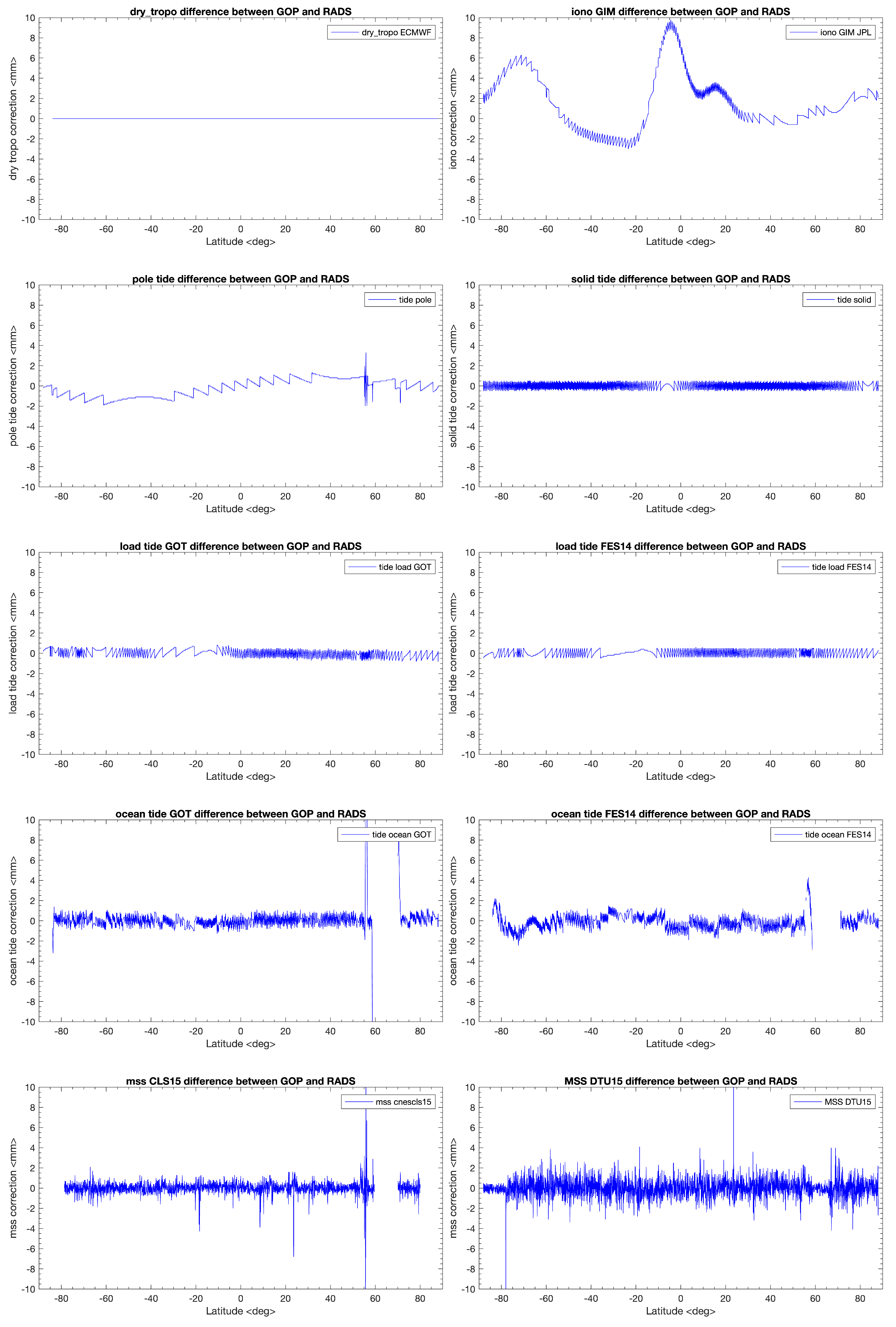
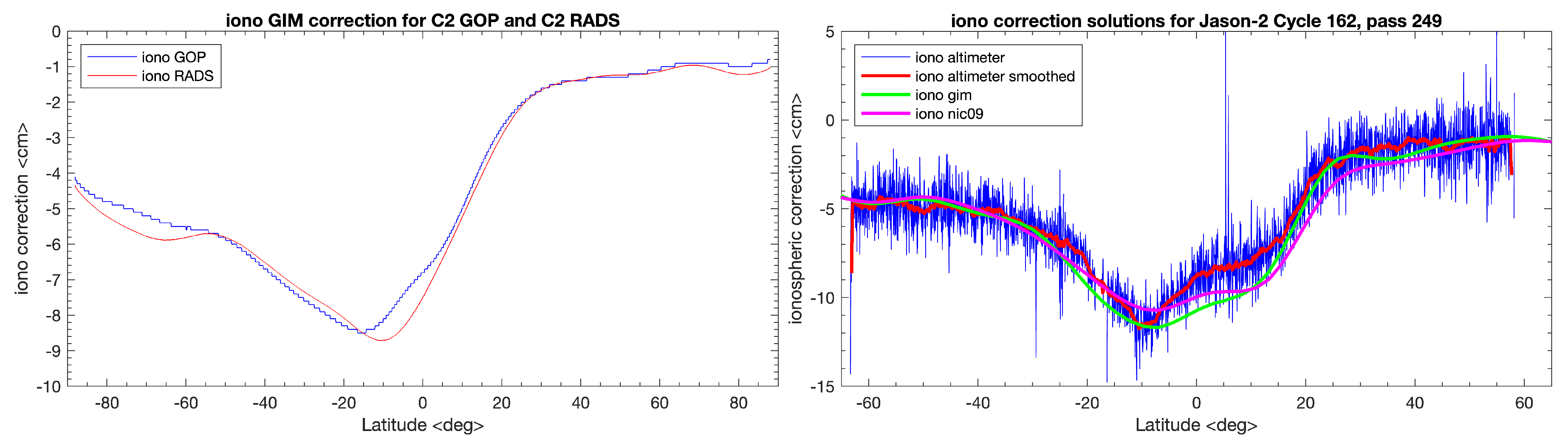
2.2. Analyzing the Corrections Needed for Sea Level Anomaly

After the conversion of all GOP data to RADS (conversion only in format, timings, and reference ellipsoid, as discussed previously), we need to validate all the corrections that are needed to generate the sea level anomaly (SLA) before starting our elaborate analyses comparing CryoSat-2 GOP SLA with other concurrent altimeter missions and comparing it with tide gauges. This corrections analysis was performed by directly comparing the RADS-formatted GOP data (CG) with the ’standard’ RADS CryoSat-2 product (C2), which is in fact GOP Baseline-C data but with most corrections replaced by corrections according to the available models in RADS (applying same models/corrections is a major asset of the RADS altimeter data base system). We like to refer to this as RADSified CryoSat. Any expected differences that can arise stem from the fact that GOP corrections have 1 mm precision, whereas RADS corrections have 0.1 mm precision, meaning that a difference (when based on the same model and an identical implementation of processing and/or interpolation) would either be zero or exhibit random noise (steps) between roughly −0.5 and 0.5 mm. Figure 1 gives an example of these differences for dry troposphere, ionosphere, pole tide, solid Earth tide, load tide (GOT410 and FES2014 models), pure ocean tide (GOT410 and FES2014 models), and mean sea surface (CLS and DTU models) corrections. The wet troposphere, dynamic atmosphere, and sea state bias corrections are left out, as they demonstrate exactly the same behavior as the dry troposphere, for which the differences are exactly zero.
A few remarkable deviations remain. In Figure 1, 2nd row, left panel, the difference in the pole tide correction raises concern due to a long wavelength with a superimposed zigzag pattern, though luckily all within a 2 mm amplitude. In Figure 1, 1st row, right panel, the ionosphere based on the JPL GIM model also exhibits quite an outstanding behavior. Here, we surprisingly find a distinct signal in the difference (not noise!), with excursions in excess of a cm, which is unexpected and hints to issues with model interpolation and/or timing. The left panel of Figure 2 shows the origin of this difference giving the respective pass curves for the ionosphere corrections for GOP (blue line) and for RADS (red line). It looks like a combination of a scaling problem and a shift along the pass. Again, when the underlying models are the same, these curves should be the same, and this signal in the difference can only be due to erroneous interpolation in one of the solutions (or when having different models). As a first check to see whether RADS is systematically off, we plotted, in the right panel of Figure 2, for an arbitrary Jason 2 track, all the available ionosphere corrections based on different models and one based on the dual-frequency altimeter. The latter (when sufficiently smoothed) represents the ’truth’ based on the dual-frequency altimeter measurement. There seems to be no clear shift along the track. However, whether RADS or GOP GIM JPL is closer to the ’truth’ remains inconclusive. The RADS implementation for the JPL GIM looks decent enough as a substitute for the smoothed iono correction based on the dual-frequency altimeter.
Two other corrections raised a bit of concern too: that for the ocean tide solutions and that for the mean sea surface solutions. They are plotted in the last two rows of Figure 1. Concerning the ocean tide, the GOT410 solution looks okay; however, the FES2014 difference between GOP and RADS exhibits a strange pattern, which again must be due to some interpolation issues. Clearly, if one has to stick to the corrections available in the GOP data, the choice for the GOT410 solution would be the obvious one and is therefore advised. Concerning the mean sea surface model, we opt for the CNES_CLS15 solution instead of the DTU15 solution, based on the fact that the standard deviation for the CNES_CLS15 difference is less than that of the DTU15 difference, though they are both below a few mm. And finally, in the left panel and 2nd row of Figure 1, we notice the peculiar behavior of the pole tide difference between GOP and RADS.
To get an idea what this along-track difference looks like around the globe, we performed a collinear tracks analysis between the GOP data corrections and the equivalent RADS-generated corrections (RADSified GOP data). By carrying this out, we are able to plot the correction differences geographically per cycle. This should reveal (problematic) patterns if they are present and might hint at how to improve the interpolation of the models/grids. By collinear tracks analysis, we can, for each point along a pass, side by side, subtract the RADS from the GOP solution. Figure 3 gives an overview of the results for cycle 34. We plotted a typical ‘no problem’ correction (here, the dry troposphere) and the ones that do appear troublesome: viz.  the ionosphere, the pole tide, the FES2014 ocean tide, and the DTU15 mean sea surface corrections. The subsatellite nadir point along track for pass 840 is drawn as well, so one may easily compare Figure 1 and Figure 3.
Basically going over Figure 3, we obtain a confirmation of the problems we saw in the along-track examples, where the ionosphere correction is still the most worrying. The top left image, again, is the typical unproblematic correction difference: low noise and no spatial patterns. Corrections like the wet troposphere, the solid tide, the load tides (GOT410 and FES2014), ocean tide for GOT410, and mean sea surface for CNES_CLS15 perform similarly to the dry troposphere corrections. The sea state bias correction also performs similarly, but that is because it was not changed in the RADSification. The rest concerns the ‘troublemakers’. The pole tide difference, e.g., exhibits a very typical low harmonic effect, suggesting that different models might have been used or wrongly implemented (static vs. dynamic?). The fact that the RADS office reported an error in the pole tide and allegedly fixed it in early 2022 is interesting, and maybe it is fixed, but it is still remarkably different from the GOP implementation. This is not directly a concern, as it is quite small ( < 1 cm), but needless to say, these ‘problematic’ corrections need attention. For instance, by insisting on a discussion between the institutes responsible for producing the GOP and RADS corrections to come forth with details on the actual implementations. Inquiry at the RADS office concerning the JPL GIM model difference between GOP and RADS reveals that SALP (Service d’Altimetrie et Localisation Precise, the altimetry and precise positioning service of CNES), which is responsible for the GOP product, has a different method for calculating TEC at altimeter height from TEC at GNSS height: they use the equations from [29], whose approach is known for its limitations. In RADS, the original JPL GIM grids are directly interpolated to obtain the TEC at GNSS height and then the data are downscaled for the various altimeter satellites at different heights with different (fixed) multiplication factors. Comparison between the GIM TEC and altimeter dual-frequency ionosphere correction showed that such a fixed scaling is sufficiently accurate, with the advantage that such an approach does not depend on the output of the IRI95 ionosphere model [30]. At the same time, this approach also leaves room for improvement, as shown in [31].
Here, in our long-term accuracy and stability study, our biggest concern is whether these corrections or correction differences contribute to an instability of the platform; in other words, do they contribute to a trend over time. To further investigate this in our collinear tracks analyses, the correction data from all records that provide a valid sea level anomaly are differenced and per cycle averaged, so that one obtains an average mean difference between GOP and RADS CryoSat-2 corrections per cycle based on each copoint, in order to be able to observe any periodicity and drift. Figure 4 gives the final result with respect to the troublesome corrections chosen in Figure 3. Fortunately, all these corrections do not seem to contribute substantially to the observed trends in sea level anomaly, so there is no direct effect on the long-term stability. Only the ionosphere and the pole tide differences seem to have a traceable drift, albeit in the order of hundredths of mm (≤0.015 mm/yr). Obviously, there should be nothing in the tides or in the mean sea surface reference that can cause any trend, which is indeed the case. Also, the means of the differences which could contribute to a bias in the range bias are negligibly small (≤1 mm). Other interesting observations concern the periodicity in both the ionosphere difference, which seems to be inversely related to the intensity of the sun spot cycle, and in the dry troposphere difference exhibiting a typical 20-month cycle, which could be related to (unmodeled) atmospheric phenomena like wind. The differences between GOP and RADS are dependent on the accuracy and timeliness of the meteorological input data. But, again, the differences are too small to be of any concern.

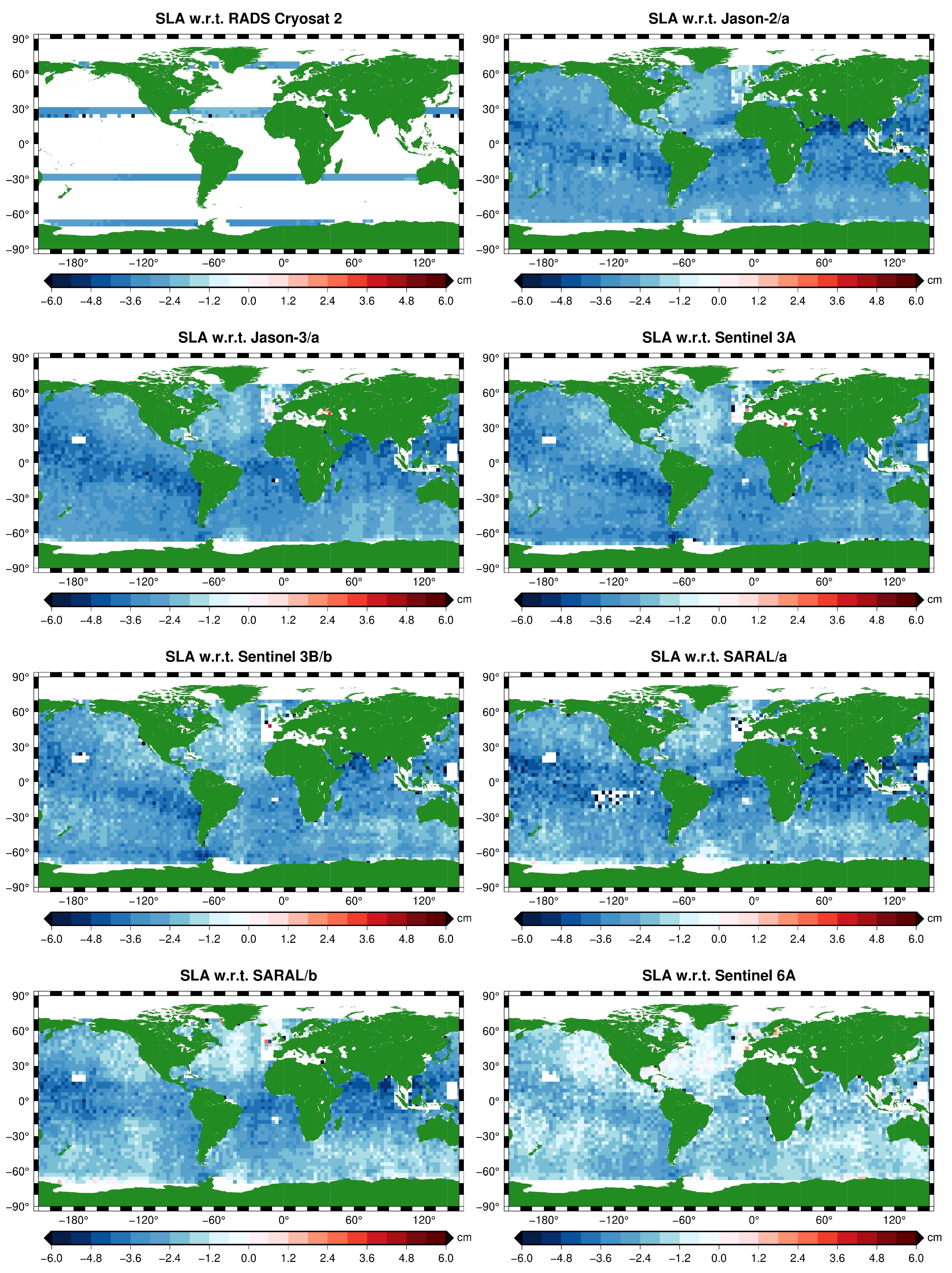
2.3. CryoSat-2 Comparison with Concurrent Altimeter Missions through Crossover Analysis

For the whole period in which we have GOP L2 Baseline-C data available, we performed crossover generation and analysis, crossing GOP CryoSat-2 passes (‘CG’) with passes from the Jason-2 phases (‘J2’), the Jason-3 phases(‘J3’), the Sentinel-3A phases (‘3A’), the Sentinel-3B phases(‘3B’) the RADS CryoSat-2 phases (‘C2’), the SARAL phases (‘SA’), and the Sentinel-6A phases (‘6A’). The reader is referred back to Table 1 for the definitions and timespans of the different missions and phases covered. The approach is similar to the one that was adapted for our GOP Baseline-B analyses [12]. We refer to this as dual-satellite crossovers (dual XOs). We also performed single-satellite crossover generation (single XOs), crossing ascending and descending passes from GOP CryoSat-2, Jason-2, Jason-3, Sentinel-3A, Sentinel-3B, RADS CryoSat-2, SARAL, and Sentinel-6A separately. The chosen maximum crossover time difference is set to 2 days. This is still considered an appropriate number, since in 2 days, not much of the actual dynamically varying sea level will change. Fewer than 2 days leaves too few crossovers in the crossing of GOP CryoSat-2 with RADS CryoSat-2. In order not to include too much ocean variability, we combined this with a 95% crossover difference edit criterion, i.e., 2 times the standard deviation, discarding no more than 5% of the total number of crossovers. In addition, to exclude areas with a possibility of sea ice presence, we limited our analyses to between 70 and + 70 latitude. Another advantage of limiting the area is excluding the large number of high-latitude crossovers which would otherwise bias the solution. These edit criteria were used for all satellites and all satellite combinations to be able to make a fair comparison. The initial rationale to compare GOP CryoSat-2 with RADS CryoSat-2 was twofold. The first is that at the time of the availability of GOP Baseline-B data, the altimeter measurements were processed differently (GOP vs. RADS), in particular the way the wave forms were retracked, so we considered it useful to compare these different products as they originate from the same source. The other reason is the different treatment of correction models. Meanwhile, as a result from the analyses on the Baseline-B product [12], it was decided to incorporate the new Baseline-C data directly in RADS to replace the earlier CryoSat-2 RADS-own product, which makes the first reason obsolete; the comparisons of the corrections are still valid though, as we learned from Section 2.2, so these correction differences remain under investigation.
The mean crossover differences between GOP CryoSat-2 and Jason-2 provides us with the bias between GOP CryoSat-2 and the calibrated Jason-2. Likewise, with the crossovers between GOP CryoSat-2 and Jason-3, we obtain the bias with respect to Jason-3. Clearly, the reference should be the same when comparing one satellite with the other: we chose the CNES_CLS15 mean sea surface as reference for all satellites and applied the GOT410 ocean tide and ocean load correction for all satellites. Comparing GOP CryoSat-2 with Jason-2 (crossover difference CryoSat-2 minus Jason-2) basically gives the range bias with respect to Jason-2, but as both have their data referenced to the TOPEX reference ellipsoid (in RADS), and a calibrated range bias was already applied to Jason-2, the actual range difference is with respect to the TOPEX reference, and it can be regarded an absolute range bias! The same is true for the other satellite missions, albeit that for some there was less time for proper calibration, which could make them be slightly off. We employed the Jasons and Sentinel-6A as reference missions, though it is interesting to follow the mean crossover difference in time between GOP CryoSat-2 and all the other missions and mission phases, including the standard RADS CryoSat-2 product.

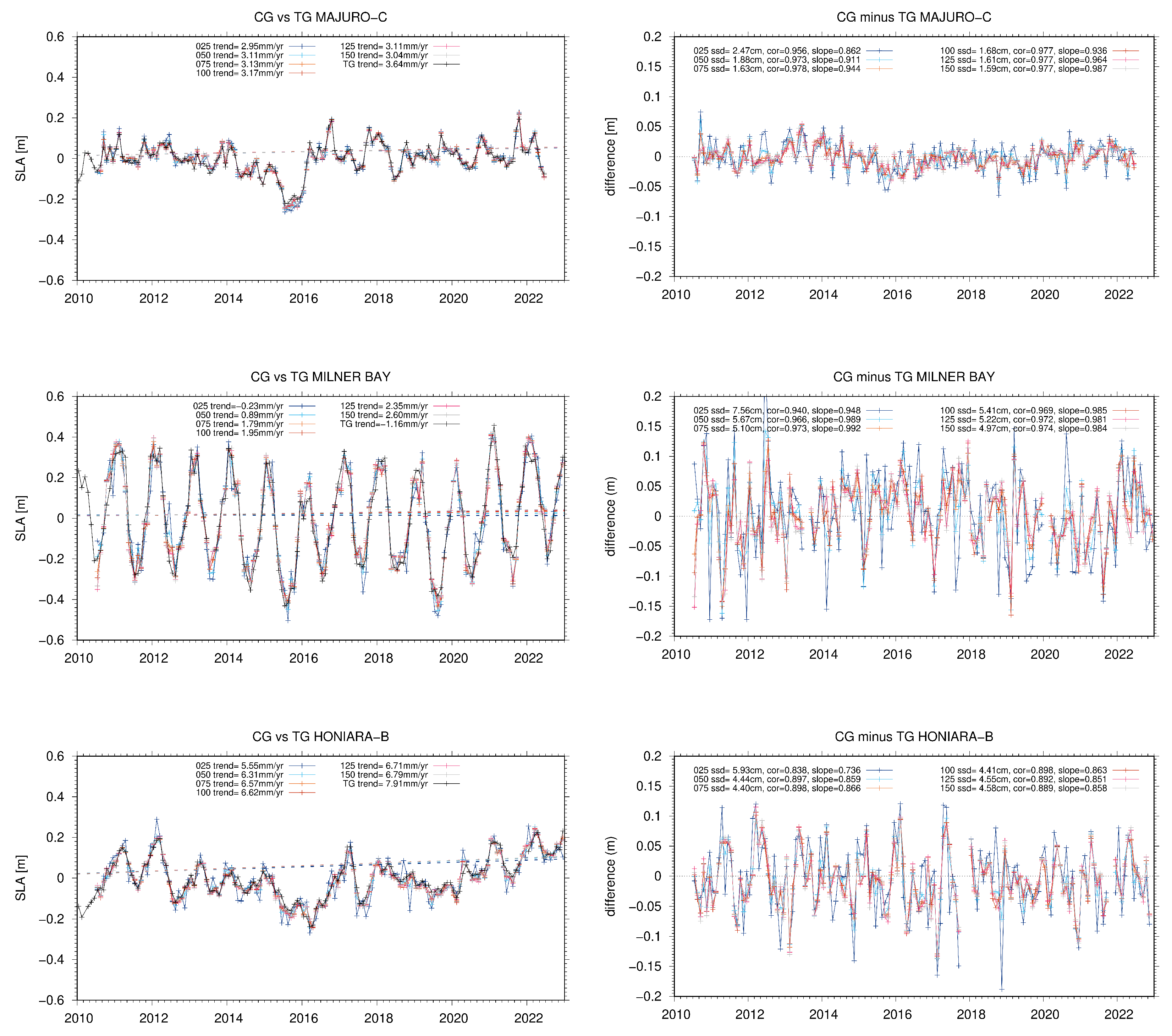
2.4. CryoSat-2 Comparison with Tide Gauges through Interpolation

For the method we employ for comparing CryoSat-2 GOP altimetry with tide gauges, we refer the reader to [12,32]. Here, it suffices to say that we now investigate Baseline-C data. To be able to compare the tide gauge data with the altimeter data, we applied all the standard corrections to the altimeter data, including the total ocean tide correction (GOT410), and referenced the altimeter data to the CNES_CLS15 mean sea surface to obtain sea level anomalies (SLA). For the dynamic atmospheric correction (DAC), we only apply the high-frequency part of MOG2D, which basically means not applying the static inverse barometer effect, because the altimeter and tide gauge ’undergo’ the same static inverse barometer. The high-frequency atmospheric forced part is needed because it aliases to much lower frequencies in the altimeter data. The resulting sea level anomaly (SLA) data were gridded to obtain monthly solutions. We applied a Gaussian distance-weighted gridding with a σ choice between 0.25 and 0.75 , a cut-off horizon of 3 σ , and a grid spacing of 0.25 . The grdtrack routine from the Generic Mapping Tools (GMT) [33] is then applied to the monthly altimeter grids to generate the SLA time series at the tide gauge station locations. The default interpolation method in grdtrack is bicubic, and it uses the geographic coordinates from the grid cells. The last step in the process is the removal of a common bias as the tide gauge data are not referenced to a known ellipsoid but rather to a locally defined mean sea level.
Before presenting the final details in Section 3, we analyze some results from applying a few different options for our gridding and interpolation method. Obviously, we want the scenario which provides the solutions from the CryoSat-2 GOP data that are the closest to the sea level data of the set of selected TG stations. Conversely, we also want to fairly compare the results from our reference missions, Jason-2, Jason-3, and Sentinel-6A. In Table 2, we analyze different σ for our distance-weighted gridding, keeping the cut-off horizon at 3 σ ; this includes our standard (‘best’) solution for the reference missions of σ = 0.5 , as well as different cut-off horizons with no σ (no distance-weighted gridding). The grid spacing for each time is 0.25 . Basically, these statistics hint towards either going for the ’075’ case or going for the ‘125’ or ’150’ case. Now, the problem with the latter two is that the tilt difference between GOP data and the TG data seems to deteriorate. This would be a vote against going for the ’125’ or ’150’ solutions, basically leaving ’075’ and ’100’ as ‘good’ cases. As in the ’100’ case the horizon is limited to 1 degree, this would leave a lot of vacancies in our grids for the reference missions (10 days repeat orbit, track spacing along the equator around 1.42 ). Then, basically only the ’075’ case would represent the best solution (in order to be able to compare GOP and the reference missions).
To be more certain concerning the gridding parameters, we check, in Figure 5, the comparison results of three of the best-performing tide gauge locations. Here, in the left panel, top to bottom, we compare CryoSat-2 GOP sea level data with the Majuro-C tide gauge, with the Milner Bay tide gauge, and with the Honiara-B tide gauge. The numbers in the legend represent the individual trend lines for the 6 analyzed altimetry gridding cases, together with those of the TG data. And, in the right panel of Figure 5, we plotted the sea level differences between CryoSat-2 GOP and the 3 tide gauges. The numbers in the legend represent the difference statistics, like sample standard deviation (ssd), correlation (cor), and linear regression trend (slope). Clearly, the right panel says more about the actual fit of the altimetry data with the TG; one should get that from the left panel as well, but then one would be looking in a qualitative manner, where the colored line follows the black line the most closely, with the dark blue line standing out as the ‘worst’ case. Back to the right panel, concerning cor and ssd, taking the common denominator into account, case ’075’ does fit best or is 2nd best on all accounts. Also, taking into consideration that cases ’100’ and ’125’ will not be okay for proper comparison with the reference missions, we finally conclude that the ’075’ case is a good all-round gridding solution and therefore is chosen for the overall tide gauge comparisons.
We tested an alternative method in which we do not grid the altimeter data to monthly mean grids but gather the data directly in the vicinity of the tide gauge location. For this, a circular boundary of 2.5 in diameter was chosen. Subsequently, the data were smoothed (Savitzky–Golay filter, degree 3) and resampled (linearly interpolated) to monthly means. The difference from the original method (gridded monthly means) is smaller than 1% for the correlations and smaller than 5% for the standard deviations. Again, we conclude that the ’075’ gridding case is sufficiently accurate for our research objectives.
After the distance-weighted gridding of the altimeter data with the selected σ = 0.75 , cut-off horizon of 3 σ , and grid spacing of 0.25 , we first select the monthly RLR (Revised Local Reference) tide gauge (TG) data available for the years 2010 up to and including 2021 from the PSMSL records [34,35]; this reduces the dataset from 1573 gauges to 565. The next step is aligning the altimetry-based SLA, for which we only considered tide gauge stations that have a correlation with CryoSat-2 GOP SLA and with the SLA from the reference missions Jason-2 and Jason-3 of R > 0.5 , an SLA−TG standard deviation of σ < 12 cm, and an SLA−TG slope of y < 6 mm/yr. The tide gauge trends were individually corrected for glacial isostatic adjustment GIA based on the information given on the PSMSL website (https://psmsl.org/train_and_info/geo_signals/gia/peltier/drsl250.PSMSL.ICE5Gv1.3_VM2_L90_2012b.txt, accessed on 1 January 2023) which is based on the ICE-5G v1.3 ice model [36]. Taking the mean for all tide gauge locations, this translates to a mean rate of GIA sea level change at 0.3 mm/yr ± 50% The GIA sea level trend was used to correct the TG time series by subtracting it from the TG sea level rate; in other words, in the difference slope (altimeter minus TG), the GIA contribution was added. Tide gauge selection based on all aforementioned altimetry comparison parameters can be a proper solution if no independent information is available on the actual tide gauge quality and when one is only looking for trends or drifts in the altimetric data. For the majority of the tide gauges, there is simply no information on vertical land motion (e.g., due to local tectonics). In addition, we also excluded stations for which either the TG or the altimetric SLA time series has too many data gaps (missing more than 14 months over the total time span of 140 months). This further reduces the dataset to 309 stations.

2.5. Final Words on Using GOP Baseline-C and Follow-Ons

The standard sea level anomaly SLA definition in RADS reads as follows:
SLA = alt rng dry wet ion dac std otd ltd ptd ssb mss rfo ,
with the usual suspects being alt  the orbital height; rng  the altimetric range; dry  the dry troposphere correction; wet  the wet troposphere correction; ion  the ionosphere correction; dac  the dynamic atmosphere correction; std  the solid tide correction; otd  the ocean tide correction; ltd  the load tide correction; ptd  the pole tide correction; ssb  the sea state bias; mss  the mean sea surface model height; and rfo  the reference frame offset or absolute bias (if any). Table 3 gives an overview of the chosen GOP components in our RADS-based analyses. The deviation of the components from the options chosen for the precomputed SSHA concerns the ocean tide model and the mean sea surface model, CNES FES2014b being the ocean, FES2014a the load tide, and DTU15 the mean sea surface. These are the defaults in RADS. Despite the superiority of the FES2014 model over the GOT410 model in coastal areas [37], for our analyses, we purposely chose the GOT410c ocean and load tide, and the CNES_CLS15 mean sea surface model corrections, because of our findings in evaluating the corrections (Section 2.2). These models, as implemented in GOP, and as implemented in RADS, behave more similarly than the other two models. Regardless, it is recommended to opt for building the sea level anomaly oneself from the components, as mentioned in Equation (1), because (a) one will have the possibility to choose different models and corrections and to leave out corrections and (b) one circumvents a found issue about the GOP prebuilt sea surface height anomaly variable ssha that appeared to be wrong for SAR and SIN mode, having substantial discrepancies with respect to LRM. It is worth pointing out that all the found limitations and issues about GOP Baseline-C data that have been reported are under investigation, and they will be corrected in the upcoming Baseline-D release of the data.
Finally, some advise for future CryoSat-2 Baselines: keep checking out new models. Meanwhile, there are some new mean sea surface models available in RADS, like DTU18, DTU21 [38], and Comb15, which combines CNES_CLS15 and DTU15 and CNES_CLS22 [39], but they have not been promoted to the RADS defaults yet. For the dry and wet troposphere ECMWF, reanalysis solutions exist (ERA) that would be more suited for long-term studies. Based on these reanalyses, the MOG2D dynamic atmosphere correction has also been reworked to an ’ERA’ solution with the same benefit for long-term analyses. We did not use these because they are not available in the original GOP product. From all our analyses, we learned that there are some corrections that need revisiting to guarantee the best product, like the ionosphere correction, pole tide correction, ocean tide correction, sea state bias (not addressed here, but be aware the SSB on GOP Baseline-C has not been tailored/optimized), range bias (ascending/descending and modes differences), and orbital height.

3. Results

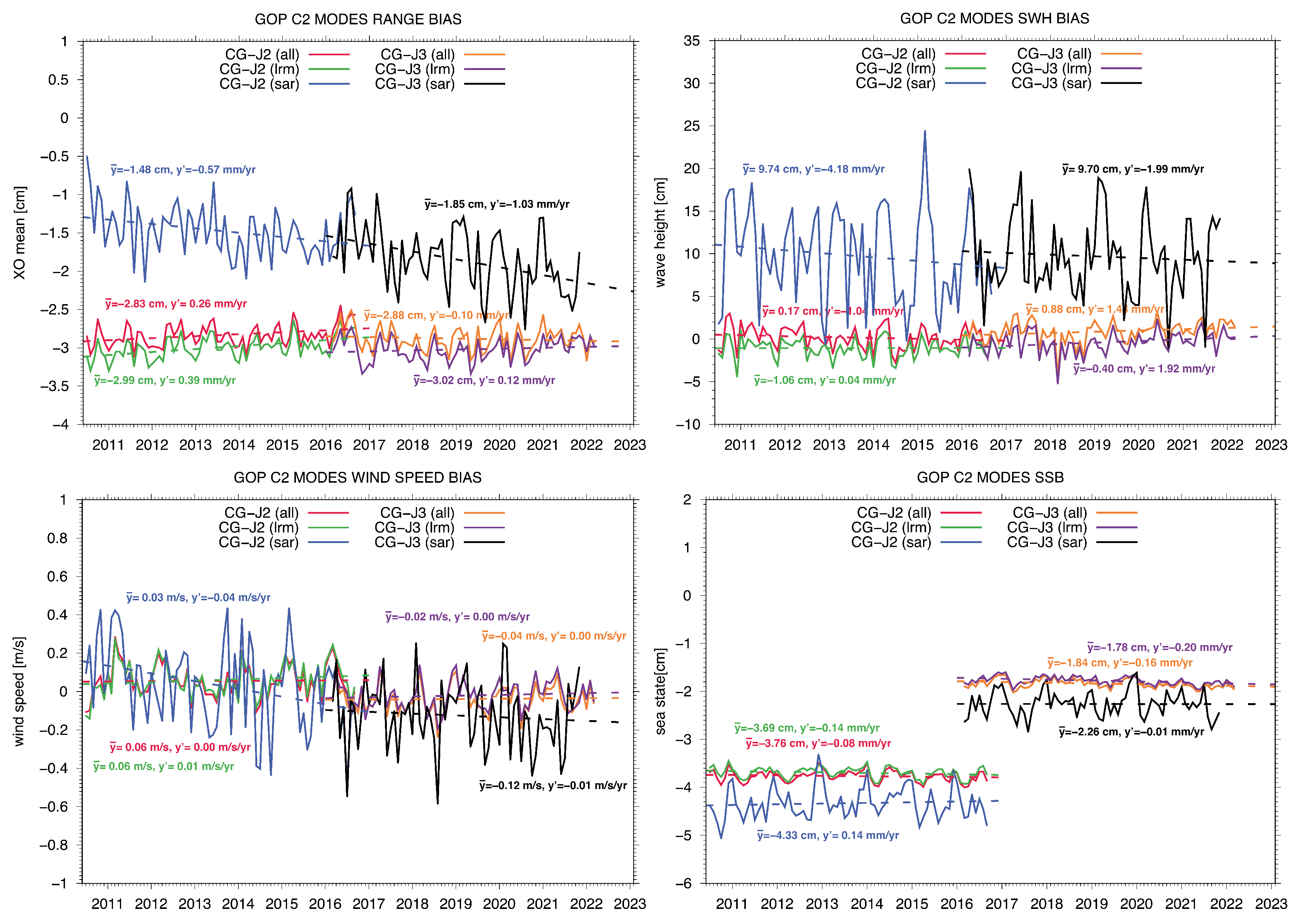
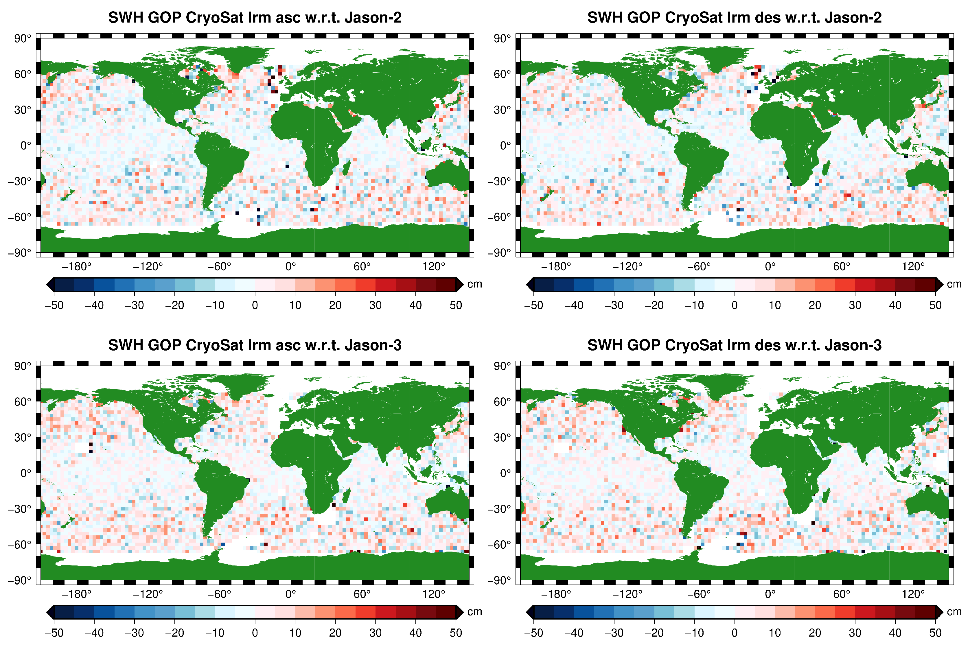
3.1. Cryosat-2 vs. Concurrent Altimetry

Figure 6 gives the result for mean crossover difference for sea level anomaly (SLA) between GOP Cryosat-2 and all the other concurrent altimeter satellite missions/phases. Due to CryoSat-2’s orbit, the number of crossovers within | Δ t | < 2 days is limited, which results in a typical banded pattern for the case where GOP CryoSat-2 crosses RADS CryoSat-2. Consecutively, Figure 7 gives the mean crossover difference for significant wave height (SWH) between GOP CryoSat-2 and the other altimeter satellites, and Figure 8 gives the wind speed (WIND). In the Supplementary Materials, Figures S1 and S2 give the results for backscatter ( σ 0 ) and sea state bias (SSB), respectively. All these plots give insight on how the biases are distributed geographically. Obviously, they are averaged over the period in which the two crossing satellites overlap (Table 1).
A few immediately striking observations from these figures can be made: In the SLA (Figure 6), we see, for all satellite comparisons, a returning SLA difference pattern around the equator, which we have already seen in Section 2.2, Figure 3, i.e., an enhanced meandering band following the inclination of the magnetic field, hinting at our ionosphere correction ‘problem’, as well as an average bias close to −3 cm. In the significant wave height SWH (Figure 7), large departures from the Sentinels and SARAL, and in the wind speed (Figure 8), typical banded differences (polar regimes), though they are absent in the differences from the SARALs.
In Figure 9, in the left panel, we plot the mean crossover difference SLA for crossing RADS CryoSat-2 with Jason-2/a and see that the equator band has more or less disappeared when compared with the GOP CryoSat-2 with the Jason-2/a solution (Figure 6, top right panel). We also applied the −2.9 cm bias to this solution, so it can be readily compared. In the right panel of Figure 9, we compare both solutions (subtracting the GOP solution from the RADS solution). In this manner, we found a way to directly compare GOP CryoSat-2 with RADS CryoSat-2 crossovers with full geographical coverage without being bothered by any range bias (it cancels out in the comparison). Obviously, this difference between RADS CryoSat-2 and GOP CryoSat-2 is a combination of the GIM ionosphere correction (equatorial band) and pole tide correction difference (a typical degree 2, order 1, Legendre polynomial pattern), as seen in Figure 3 in the top right and center left panels. From this, we conclude that the ‘problem’ of the ionosphere is in either all RADS data or just in the GOP data, and this agrees with the observation in Section 2.2 that we are dealing with different implementations of the GIM ionosphere correction model.
Table 4a provides the overall crossover statistics from the dual-satellite crossover analyses: obviously, they match with Figure 6, Figure 7 and Figure 8, and we added the statistics for backscatter ( σ 0 ) and sea state bias (SSB). Finally, Table 4b provides, for the same data products and data fields, the single-satellite crossover statistics. The last column in the tables provides the number of crossovers involved (after editing). We conclude that the GOP CryoSat-2 product is of similar quality as the Jasons, and it also closely follows the Sentinels and SARAL. The only difference standing out when going back to Table 4a is the average SLA (absolute) range bias of −2.9 cm, which is based on the average GOP SLA differences with the other satellites that have the longest phases, but leaving out SARAL, which has another type of altimeter instrument, and leaving out Sentinel-6A, which has too much of a deviating SLA XO mean. Knowing that for baseline-B we found −6.3 cm, we conclude that the GOP product absolute bias has been improved by 3.4 cm by a welcome change in ground processing. The overall sd of GOP XO differences is established at 3.7 cm, perfectly on par with the internal consistency (sd) of Jason-2 and Jason-3. Also, we see important improvements in the average biases for σ 0 and wind speed. All in all, the statistics for Baseline-C improved substantially upon an already well-performing Baseline-B product.
Let us now take a closer look at the different biases and how they evolve over time. In Figure 10, we plotted, from left to right and from top to bottom, the monthly global averages from our dual-satellite crossover analyses (mean XO differences) for seven altimetric parameters: the timing bias, the sea level anomaly (range) bias, the SLA bias standard deviation (rms XO differences), significant wave height (SWH) bias, backscatter ( σ 0 ) bias, wind speed bias, and sea state bias (SSB). For the GOP CryoSat-2 biases with respect to the reference missions (Jason-2, Jason-3, and Sentinel-6A) and with respect to RADS CryoSat-2, the values of the long-term average and trends are given in, respectively, red, orange, pink, and yellow. Obviously, the long-term averages match the values in Table 4a. The timing bias, based on minimization of the rms of GOP CryoSat single XO differences (more details in [12]), has an overall average of +0.367 ms with a slight rise over time (Figure 10, top left), which averages to zero when this is applied to the GOP data (Figure 10, top right). This is a change compared with the result from our Baseline-B analyses, indicating a change in the ground processing. In the left panel of the 2nd row of Figure 10, we see the SLA mean crossover difference in GOP CryoSat-2 with respect to Jason-2 (red curve, average of 2.83 cm), with respect to RADS CryoSat-2 (yellow curve, average of 2.90 cm), with respect to Jason-3 (orange curve, average of 2.88 cm), with respect to Sentinel-6A (pink curve, average of 1.80 cm), and with respect to the other satellites (Sentinel-3A and 3B, respectively, green and blue curves, and SARAL phase a and b, respectively, purple and black curves). With all this information, we can pinpoint the absolute range bias of the GOP data at 2.9 cm. The drift in the range bias with respect to Jason-2 amounts to 0.24 mm/yr, with respect to Jason-3 to 0.10 mm/yr, with respect to RADS CryoSat to 0.06 mm/yr, and with respect to Sentinel-6A to 0.54 mm/yr. Taking into account that the GOP-RADS difference basically only hints at ‘problematic’ range corrections (and not to the altimeter or platform itself), and that for Sentinel-6A, the time span is too short for a statement on the long term, we can say that compared with Jason-2 and Jason-3, GOP CryoSat-2 Baseline-C is excellently stable over time (averaging −0.07 mm/yr) and significantly better than the constraint of 0.5 mm/yr for an altimeter to have SLA considered an essential climate variable ECV (https://climate.esa.int/en/evidence/what-are-ecvs, accessed on 1 September 2023). In the dual XO rms (right plot, second row), we see the confirmation of the quality of the stability, averaging 3.7 cm, in line with the internal consistency of our Jason-2 and Jason-3 reference missions (compare with Table 4b). The stability is also on par with the current general uncertainty in sea level trend estimates (<0.4 mm/yr). All the mean biases, either in SLA, SWH, σ 0 , wind speed, or SSB, confirm the earlier figures and tables. Obviously, there are jumps in σ 0 and wind speed when, for instance, switching from Jason-2 to Jason-3. Basically, that is not of direct concern for the GOP product because any jumps in σ 0 and, by that, in wind speed, are ’fixed’ (discounted) in the optimized sea state bias model.
Knowing that GOP is quite stable, CryoSat-2 can function as a stable reference as well for other satellites, for instance, for the two SARAL phases a and b and for Sentinel-6A. From the tables and Figure 10, we learn that GOP has a range bias of 2.9 cm and that the average bias between GOP and Sentinel-6A is 1.8 cm, thus subtracting the 1.8 cm from the 2.9 cm gives Sentinel-6A the absolute range bias of 1.1 cm (also because in RADS there is no range bias established yet, and nothing (0 cm) is applied in RADS to Sentinel-6A by default). Applying this 1.1 cm absolute bias value to the Sentinel-6A data, we can extend our reference mission series Jason-2/Jason-3 to Jason-2/Jason-3/Sentinel-6A.
The large positive trends in the SARAL phases a and b SLA with respect to GOP, and also with respect to Jason-2 and Jason-3, in the left panel of the second row of Figure 10 are worrying. So, this seems to be an isolated problem in the SARAL data. We think these results warrant further research into the SARAL altimeter data. This is out of the scope of this paper, but we see similar behavior in the backscatter (negative trend) and wind speed (positive trend). Another concern is the SLA difference in GOP and Sentinel-3A and Sentinel-3B that suddenly starts rising halfway through 2022. The direct question of course would be if there is something wrong with the GOP data after this date. Whereas the difference in GOP SLA with respect to Jason-2, Jason-3, and even Sentinel-6A, doe not show this behavior and hints to a problem with the Sentinel-3 data, the actual answer comes from the wave height plot and the sea state plot of Figure 10:, revealing jumps in Sentinel-3A and Sentinel-3B data of 6 cm in wave height and 1 cm in sea state bias, starting approximately in June 2022. Again, with the help of GOP CryoSat-2 data, another altimeter problem has been uncovered. To be absolutely sure that there is no degradation of GOP CryoSat-2 after 2022, we performed an extra analysis with respect to a selected set of PSMSL tide gauges, for which the reader is referred to Section 3.3.1. The overall conclusion is that CryoSat-2 GOP has no apparent drift with respect to tide gauge sea levels, not even after 2022 upon close inspection.
A final remark on the range bias between the two CrySat-2 products, the GOP and the RADS version, which we already stated that in essence only deals with the correction differences: from the green curve in the left hand plot of the 2nd row of Figure 10, we observe a negligible trend ( 0.06 mm/yr), concluding that both the ionosphere correction and pole tide correction issues do not degrade CryoSat’s stability whatsoever.

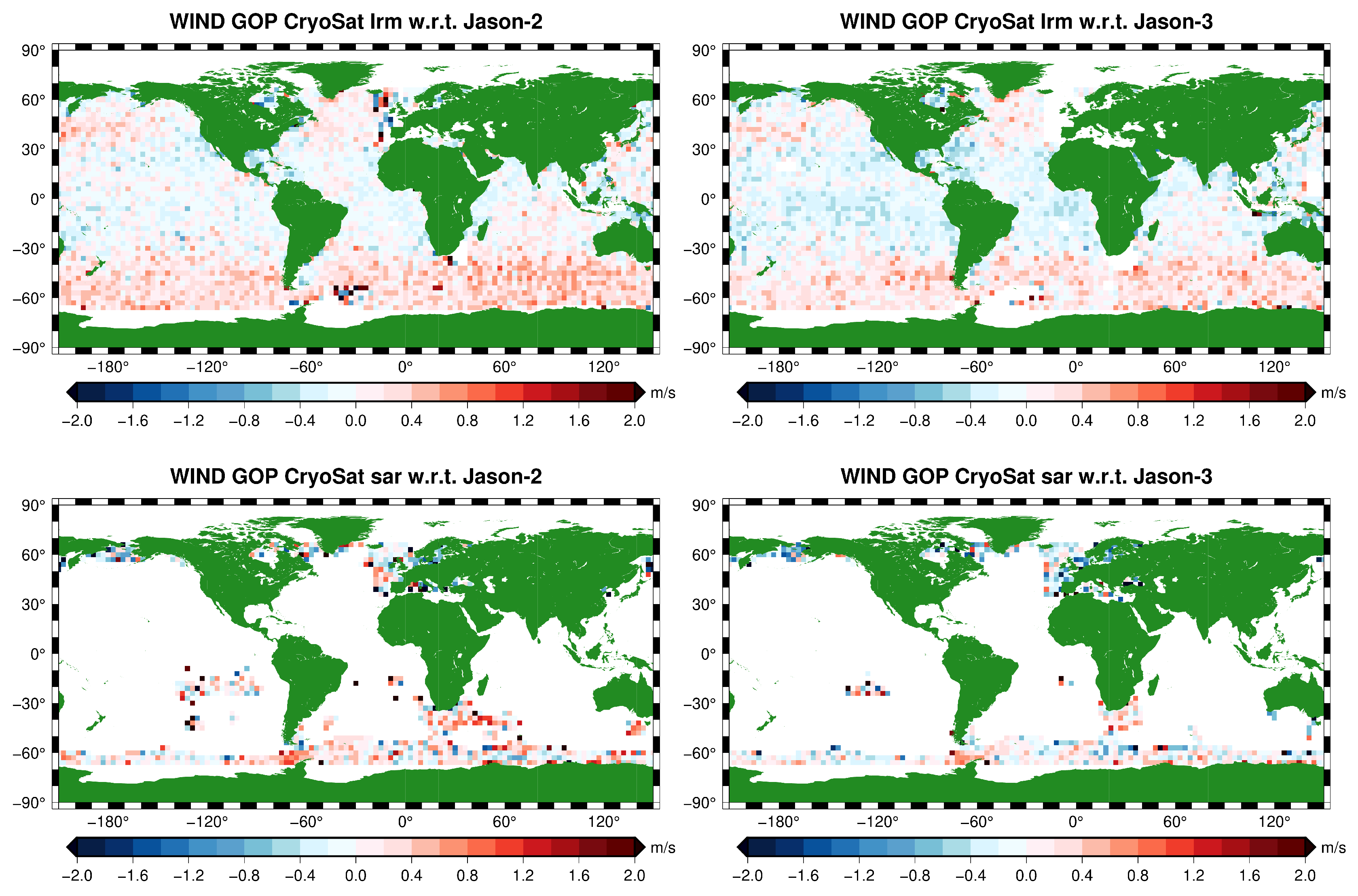
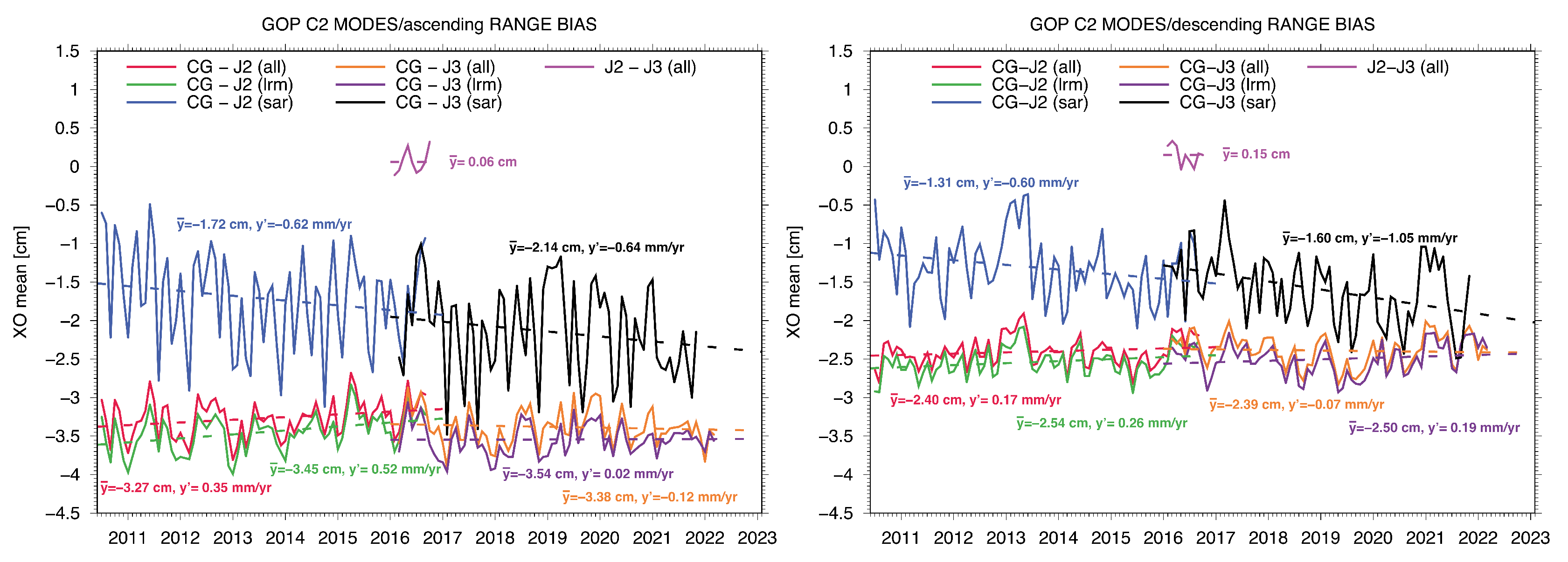
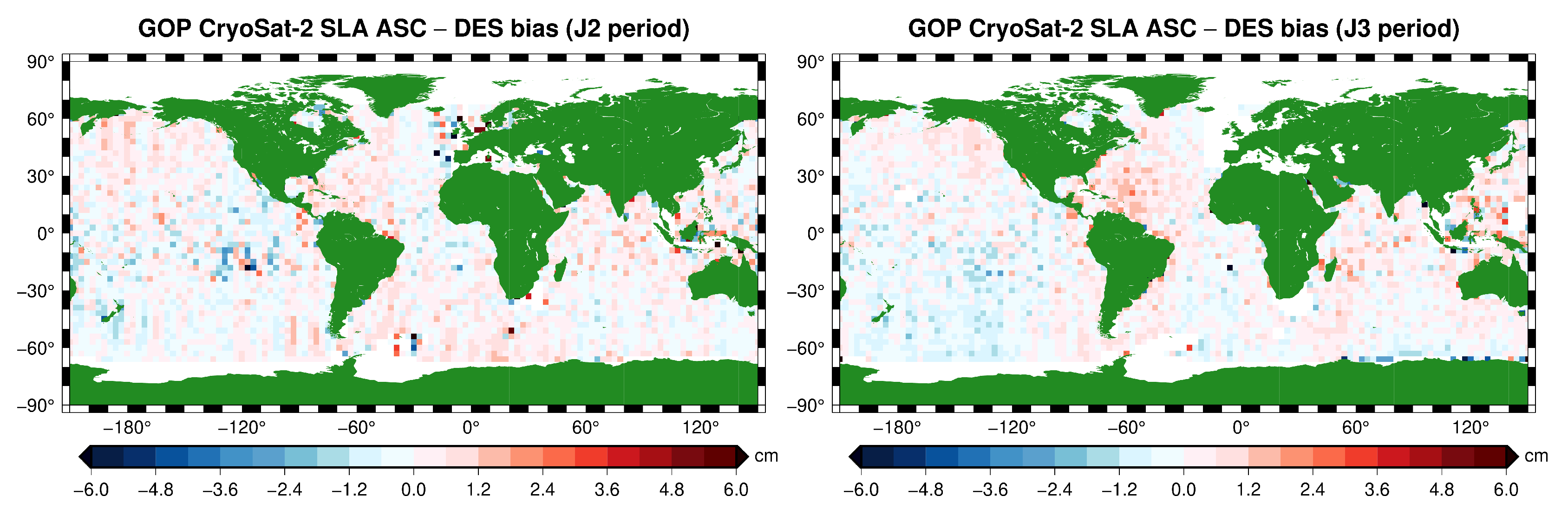
3.2. CryoSat Modes and Descending/Ascending Pass Bias

As we mixed LRM and SAR mode in our previous bias analyses, it is interesting to reanalyze the bias but now separated into CryoSat’s Low-Resolution Mode (LRM) and Synthetic Aperture Radar (SAR) mode. In Figure 11, Figure 12 and Figure 13, we plotted similar geographical maps of the mean crossovers of CryoSat-2 GOP (only with respect to Jason-2 and Jason-3), as in Figure 6, Figure 7 and Figure 8, but now for the two different modes, respectively, for sea level anomaly SLA, significant wave height SWH, and wind speed WIND. Obviously, the LRM solutions resemble the earlier combination of LRM and SAR, as the SAR mode is geographically limited. The thing to notice here is the differences between the LRM solutions and SAR solutions. For instance, in Figure 11, we see that the SLA mean XO differences on average are lighter blue for SAR than for LRM, indicating a bias between LRM and SAR SLA (positive when subtracting LRM from SAR). We observe something similar for the wind speed (Figure 13), but it is less prominent, and again, it is more pronounced for the significant wave height (Figure 12) (darker red for SAR, meaning a positive bias subtracting LRM from SAR). The main purpose of these geographical distribution maps is to see whether there are striking patterns. For this, we refer the reader back to our earlier maps and discussion on ’all’ (LRM plus SAR) solutions in the previous section.
To obtain some statistics on the mode biases, we again investigate their evolution over time. In Figure 14, we plotted, from left to right and from top to bottom, the monthly global averages from our dual-satellite crossover analyses (mean XO differences) for four altimetric parameters: the sea level anomaly (range) bias, the significant wave height (SWH) bias, the wind speed bias, and the sea state (SSB) bias. For the GOP CryoSat-2 biases, the long-term average and trends are given, respectively, in red (all), green (lrm), and blue (sar) with respect to the reference mission Jason-2, and, respectively, in orange (all), purple (lrm), and black (sar) with respect to the reference mission Jason-3. Looking at the top left panel of Figure 14, we can conclude that in the comparison with Jason-2, GOP CryoSat-2 has an SAR-LRM range bias difference of (−1.5) − (−3.0) = 1.5 cm and with Jason-3 of (−1.8) − (−3.0) = 1.2 cm. On average, this gives a 1.4 cm SAR-LRM range bias, taking into account that there is a 1 mm range bias difference between the two Jasons. Looking at SWH (top right panel), we also observe a clear difference between SAR and LRM: (9.7) − (−1.1) = 10.8 cm in the comparison with Jason-2, and (9.7) − (−0.4) = 10.1 cm with Jason-3. On average, this implies a 10.5 cm difference in significant wave height. For wind speed, we do not find any significant SAR-LRM difference, but the SWH difference must have an influence on the sea state bias, especially when the sea state bias is not optimized (otherwise, an offset would be discounted in the sea state bias model). In the bottom right panel, giving the result for SSB, we observe an SAR-LRM difference of (−4.3) − (−3.7) = −0.6 cm for the Jason-2 comparison and (−2.3) − (−1.8) = −0.5 cm for Jason-3. Apparently, the SAR-LRM offset in GOP SWH still leaves a trace in the SSB of around 0.5 cm, basically explaining 0.5 cm of the 1.4 cm SAR-LRM offset in GOP SLA. As most other corrections are close to identical, we think that the remaining difference of 0.9 cm has a different origin; it could be due, for instance, to the fact that different retrackers are used for the different modes.
However, further investigation of the biases also revealed a difference between ascending and descending passes. This is an odd finding. Figure 15 and Figure 16 represent the geographical distribution of the mean XO differences between GOP CryoSat-2 and the Jason-2 and Jason-3 reference missions, but now a distinction is made between only ascending GOP passes and only descending GOP passes. Here, we use the LRM solution (close to the ‘all’ solution), intentionally, in order to not mix modes and treat the ascending/descending difference independently from the modes bias. We plotted it for SLA in Figure 15 and for SWH in Figure 16. Obviously, in the former figure (SLA), there is a clear ascending north–south pattern that is reversed for descending passes (for Jason-3, similar to Jason-2), and for the latter figure (SWH), obviously not. So, we are dealing with a phenomenon that is only on the sea level. Figure 17 reveals the evolution of the monthly means over time. With this, we get an idea of the actual bias values and trends involved. We plotted all the bias distinctions we can make with respect to modes and with respect to ascending/descending passes: left, the ascending case, and right, the descending case. We discern all GOP with respect to Jason-2 (red), LRM GOP with respect to Jason-2 (green), SAR GOP with respect to Jason-2 (blue), all GOP with respect to Jason-3 (orange), LRM GOP with respect to Jason-3 (purple), and SAR GOP with respect to Jason-3 (black), and we also added Jason-2 with respect to Jason-3 (only along the reference tracks when they simultaneously flew the same tracks, which was for about 7 months) for comparison purpose (in pink). This comparison between Jason-2 and Jason-3 shows us that there is not more than a 0.1 cm asc/des difference between Jason-2 and Jason-3, which is negligible. The left panel of Figure 17 teaches us that the ascending range bias for LRM is about −3.5 cm, whereas the descending range bias for LRM is about −2.5 cm, a difference of approx. 1 cm. The strange behavior of the blue and black (SAR) lines (obvious trend and less ascending/descending difference) is not fully understood but must come from the limited coverage of the SAR mode patches and the changes in patch locations over time.
Figure 18, finally, takes the ascending and descending pass range bias and significant wave height bias differences in GOP CryoSat-2 LRM data with respect to Jason-2 and Jason-3 (the results are displayed in Figure 15 and Figure 16) and subtracts the descending result from the ascending result: top left (Jason-2) and top right (Jason-3). Basically, the names ’Jason-2’ or ’Jason-3’ might give rise to misinterpretation: both the ascending and descending solution are given with respect to, e.g., Jason-2, and subtracting them cancels out Jason-2 in the equation, and likewise, with the solution given with respect to Jason-3, Jason-3 cancels out in the subtraction. To put it differently, the left and right panels should be the same, and indeed, they look almost identical, the only difference being the different time frames or periods (Jason-2 time frame, 100703–160901, and Jason-3 time frame, 160303–220303). One could argue that we could have obtained the same answer if we would have used the CryoSat-2 single crossovers directly, as this would also look at the difference in ascending and descending tracks, and Table 4b suggests a 0.7 cm bias, but we would obtain the same banded geographical distribution as the ones from crossing GOP CryoSat-2 and RADS CryoSat-2 in, e.g., Figure 6, and we would not be able to actually see the north–south pattern so clearly. Increasing the allowable crossover time difference would improve the geographical distribution but would pollute the result with all kinds of sea level variability. So, we think that with this, we present the most clear way of revealing the ascending/descending problem of GOP Baseline-C data. In the bottom left panel of the figure, we added the ascending minus descending solution for GOP CryoSat-2 SWH (Jason-3 timeframe), and for comparison reasons, in the bottom right panel, we added the Jason-2 SLA ascending minus descending solution (for the Jason-2/Jason-3 overlapping timeframe). In this Jason vs. Jason case, there is no substantial bias left (<0.1 cm), and no particular patterns are visible. This also holds for the GOP CryoSat-2 significant wave height, so we conclude that the ascending/descending bias issue is only in the sea level anomaly and not in any of the other altimetric parameters. And, it is also not in the SSB, because we do not see it in the SWH.
Going back to the top panels, this ascending/descending bias in the sea level anomaly exhibiting a clear north–south pattern is quite an astonishing result, and it seems to represent a zonal degree 1 (spherical harmonics) issue. This ascending/descending offset can be represented by a C10 coefficient, which is directly related to the z-component of the geo-center or center of the earth’s mass. This would suggest a problem with centering the orbit for CryoSat-2, which cannot be due to the Earth gravity model used but rather to a geometric offset introduced by the tracking data. On the other hand, a z-shift in the center of mass of the earth would not contribute to crossover differences between ascending and descending passes: the location of the crossovers might be changed, but it would not matter from what direction one would pass this new location [40]. Another explanation was sought in the fact that the orbit is not completely frozen, but this is taken care of by the precise orbit determination. What does has an influence on differences between ascending and descending passes is a timing or datation bias: together with the orbital rate, a timing bias would generate a pseudo- (erroneous) elevation, different for the ascending and descending passes. This has been reported in [4], albeit for Baseline-B, for which the timing bias was smaller and less of an influence on the data. Through transponder calibration, the timing issue should have been dealt with in Baseline-C [18], so we refer back to Section 3.1, Figure 10, where a timing bias of +0.367 ms was determined. As we report on Baseline-C data as they are provided by ESA, we did not apply (remove) this timing bias from the GOP Baseline-C dataset for our analyses (and we also did not apply the found range bias either); we merely report on it. But, if we apply the found timing bias, we obtain the result in Figure 19. Comparing this result with the top panel of Figure 18, we see that the north–south pattern has completely disappeared, and we conclude that we found the wrongdoer in the form of the datation misfit. As this ascending/descending bias problem seemed solved, no further investigation was needed.
In summary, concerning biases, we state that from the SAR-LRM bias of approximately 1.4 cm, on average, about 0.8 to 0.9 cm can be explained from the ascending–descending bias (in the global distribution one can see that there are more SAR data in the Southern Hemisphere than in the Northern Hemisphere). The remaining 0.5 to 0.6 cm bias comes from the SSB SAR-LRM bias, which in turn comes from the SAR-LRM bias in the significant wave height of around 10.5 cm, and the latter can be considered a ‘retracker’ bias, or at least a bias in the SWH generation in one of the two different retrackers (SAR vs. LRM).

3.3. Cryosat-2 vs. Tide Gauges

As explained in Section 2.4, we selected 309 PSMSL tide gauge stations that survived our outlier detection requirements and analyzed the statistics of the differences in GOP CryoSat-2 (CG) SLA with the sea level data at the tide gauges. Alongside this, we carried out the same analysis for our reference mission series Jason-2/Jason-3 (REF) and checked the differences with the same set of tide gauges. Figure 20 provides the map with the 309 locations of the selected set of tide gauges (light-blue place markers). Ahead of the actual results, the light-green place markers indicate the best six solutions on the basis of correlation.
For GOP CryoSat-2, this statistical analysis resulted in a mean correlation of R = 0.82, a mean standard deviation of σ = 5.7 cm, and mean tilt of the CG−TG difference of 0.17 mm/yr, which nicely fits within the 0.24 mm/yr and −0.10 mm/yr drift values with respect to Jason-2 and Jason-3 found before in Section 3.1. Basically, we can already draw the conclusion that the CryoSat-2 GOP Baseline-C product is extremely stable (note that we analyze the difference between tide gauge and altimetric sea level, so any ’natural’ sea level rise would be seen by both and cancel out). It is hard to tell exactly where a remaining rate between the tide gauges and altimetric sea level could come from, but it could of course be (partly) due to local vertical land motion. On top of that, one has to realize that the averaged global MSL rate has a ±0.4 mm/yr uncertainty [41].
For the reference missions REF, we found a mean correlation of R = 0.84, a mean standard deviation of σ = 4.9 cm, and a mean tilt of the difference of −0.11 mm/yr (REF−TG). Table 5 summarizes the results. The average difference in common bias removed (CG−REF) amounts to 1.7 cm, which is not the same value as we found as the range bias in Section 3.1; remember that the crossover analysis is global and covers many more data points, whereas our tide gauge stations are sparse and not evenly distributed but rather close to land and islands, so the average common bias is not a global average and cannot be used as a ‘range bias’.
In Figure 21, we plotted the six best GOP CryoSat-2 and Jason-2/Jason-3 (REF) tide gauge comparisons (light-green place markers in Figure 20). The individual statistics for the 309 tide gauges can be found in Table S1 of the Supplementary Materials. Checking in detail the differences in how both GOP CryoSat-2 and Jason-2/Jason-3 follow the tide gauge data, we conclude that Jason-2/Jason-3 outperforms the CrySat-2 GOP Baseline-C product, as expected, because of REF’s better temporal resolution (10-day repeat cycles vs. 30-day drifting cycles), but that the differences are so small that GOP can be classified to be on par with the reference missions.

3.3.1. Drift after 2022

In order to be able to conclude whether the CryoSat-2 GOP data are drifting away from the reference, as was suggested in Section 3.1 on the basis of a drifting GOP with respect to Sentinel-3A and Sentinel-3B, we extended the tide gauge comparison beyond 2021 (up to 2023) for our six best solutions. The results are given in Figure 22. Next to the CryoSat-2 GOP (CG) comparison with the tide gauges, we also added the tide gauge comparison with CryoSat-2 RADS (C2), with the sequence of Jason-2, Jason-3, and Sentinel-6A (REF), as well as with Sentinel-3B (3B). The reference mission (REF) was previously defined as the sequence Jason-2–Jason-3, but it has been extended with Sentinel-6A (all following the original TOPEX cycles). For this, we applied a −1.1 cm bias, which was found with the ’help’ of GOP CryoSat-2, as discussed previously in Section 3.1. Clearly, in Figure 22, we find no evidence for GOP drifting away from the tide gauges, nor for RADS CryoSat-2, nor for REF. Oppositely, this is also not obvious from the Sentinel-3B result. It is stressed, however, that, in our tide gauges comparison, we are looking at the cm level, whereas in the plot of the time evolution of SLA range bias (Figure 10), we are looking at the mm level. Meanwhile, referring back to Section 3.1, we found the cause for the alleged deterioration of GOP with respect to Sentinel-3A and Sentinel-3B after 2022, i.e., jumps in the SWH crossover differences in Sentinel-3A and 3B, leading to jumps in the sea state bias and consequently jumps in the sea level anomaly. Suffice it to say that GOP is so stable that it actually can be adopted as a reference to other missions (remember, we used the XO comparison of GOP with respect to Sentinel-6A to adjust the bias of Sentinel-6A to get it perfectly aligned with the Jason-2–Jason-3 sequence). The GOP CryoSat-2 tide gauge comparison falls short a bit though, like the REF result, when we analyze Sentinel-3B: on numerous occasions, the correlation with the tide gauge is better, as the standard deviation std is smaller, apparently making Sentinel-3B better-suited for tide gauge comparisons. When every operational mission is sufficiently calibrated and validated, the combination of concurrent satellites will obviously give the best sea level results, and CryoSat-2 has proven to be a worthy companion in this operational mix.

4. Discussion and Conclusions

In this section, we highlight all our important findings from Section 3 dealing with the long-term ocean data analysis and validation of CryoSat-2 GOP Baseline-C data. We learned that more than 12 years worth of CryoSat-2 GOP Baseline-C data compare very well with the data from Jason-2 and Jason-3, our established reference missions during the lion’s share of the CryoSat-2 Baseline-C period, and are very well suited for oceanographic applications. They also compare well with Sentinel-3A, Sentinel-3B, SARAL, RADS CryoSat-2, and Sentinel-6A, the other concurrent altimeter missions. And the CryoSat mission is still going strong, showing no deterioration, though it is good to know that CryoSat-2 will have an even better successor mission in the frame of the expansion of the Copernicus Space Component program of ESA, named the Copernicus polaR Ice and Snow Topography ALTimeter mission (CRISTAL) [42], which is scheduled for launch in 2027.
The CryoSat-2 GOP Baseline-C product has a slowly increasing timing error with an average of +0.367 ms, which could be accounted for but does not have a significant effect on data stability. Concerning the metadata of the NetCDF product, we stumbled on frequent erroneous ascending flags, which were dealt with by using the sign of the latitude difference between the first and last measurements of a pass. Furthermore, GOP Baseline-C correction parameters exhibit noteworthy deviations with respect to corrections produced by the RADS tools for pole tide, ocean tide FES2014, GIM ionosphere, and DTU15 mean sea surface. Patterns indicate either interpolation errors, processing errors, or still different models or implementations used. We recommend the end-user of Baseline-C data builds their own sea level anomaly (thus not using ssha) and chooses the ocean tide GOT410 and the CNES_CLS15 mean sea surface for having the least issues. If one insists on applying FES2014, we recommend applying FES2014 externally from a trusted source or using the CryoSat-2 data in RADS instead. This will not change the results presented in this paper outside their error margins, as we saw in Section 3 that the differences in CryoSat-2 GOP with CryoSat-2 RADS are marginal. It is important to provide correct (precise) model and reference in the global attribute “source” and “comment” of any variable in the data, be it in the GOP or the RADS data, to support detailed analyses by the end-user. Though some of the corrections exhibit deviations from the RADS-generated corrections, none of them proved to contribute to the overall observed trends. They are all well under 0.015 mm/yr. Also, their average contribution to the range bias is below 1 mm.
From our extensive crossover analyses with all concurrent altimeter missions, we established a range bias of the GOP Baseline-C data of −2.9 cm. This is with respect to the Jason-2–Jason-3 sequence of reference missions and also when averaged over most of the other concurrent altimeters. As all altimeters have been put in the TOPEX reference frame and all (but Sentinel-6A) have a calibrated range bias applied, this Baseline-C range bias is in fact the range bias with respect to the TOPEX reference ellipsoid and can be regarded as the absolute bias. We also established no substantial drift (<0.2 mm/yr) in this bias, which leads to the conclusion that GOP Baseline-C provides a very stable measurement and, as such, can measure up to the quality of the reference missions. With this knowledge, we used CryoSat-2 GOP Baseline-C data as a reference for the Sentinels, especially Sentinel-6A, for which in RADS no range bias has been established yet. By doing so, the crossover analyses comparing GOP Baseline-C with Sentinel-6A data reveal a −1.1 cm absolute range bias for Sentinel-6A. Applying this bias to Sentinel-6A enables the extension of the TOPEX–Jason-2–Jason-3 reference sequence to TOPEX–Jason-2–Jason-3–Sentinel-6A, a solid reference following the original TOPEX tracks for more than 30 years!
The CryoSat-2 GOP Baseline-C range bias, when separated in SAR mode only and LRM only, shows a jump of 1.4 cm, which for one part is due to an SAR-LRM bias in the sea state bias correction of 0.5 cm and, for the other part, to an 0.9 cm range bias between ascending and descending passes. Upon closer inspection, we discovered that the 0.5 cm range bias difference between GOP LRM and SAR comes from a substantial SAR-LRM bias difference in the significant wave height of 10.5 cm. Knowing that the sea state bias correction has not been optimized/tailored for CryoSat-2 GOP, the sea state bias model will not resolve any significant wave height bias issue, which will get through to the sea level anomaly. Back to the Baseline-C range bias in the difference between ascending and descending passes: it shows a very clear one-degree zonal-banded north–south pattern, which we found to be due to a datation bias in the orbital position of CryoSat. Performing the ascending and descending comparison through crossovers with the reference mission Jason-2 and Jason-3, we were able to clearly visualize this geographic pattern. When ascending and descending passes are combined, this pattern obviously diminishes, but another (less prominent) pattern remains in the east–west direction, which we believe must be due to an issue with the pole tide. The north–south pattern totally vanishes when we apply the found +0.367 ms timing bias.
From our in situ comparisons between CryoSat-2 GOP Baseline-C and the selected set of 309 PSMSL tide gauges that met our quality requirements and span the period 2010–2022, we derived a correlation of R = 0.82 and a mean standard deviation σ = 5.7 cm between the altimetric sea level and that from the tide gauges, having removed a common reference/bias and applied the GIA according to Peltier’s ICE-5G 1.3 ice model. Zooming into the bias evolution over time, on average, we can state that CryoSat-2 GOP Baseline-C has a drift of 0.17 mm/yr with respect to the tide gauge data. Again, as already became clear from the crossover analyses with the other altimeter missions, this insignificant drift indicates a very stable measurement in terms of reference frame drift. This is definitely on par with the reference missions Jason-2–Jason-3 (REF), which showed a correlation of R = 0.84, an sd of σ = 4.9 cm, and a drift in the difference of −0.11 mm/yr with respect to the same set of tide gauge stations. Both values, in an absolute sense, for Baseline-C and REF, fall within the 0.4 mm/yr accuracy of current altimeter missions. We therefore conclude that GOP Baseline-C has no apparent drift with respect to tide gauge sea level. Also, after 2022, no drift was spotted when we investigated an extended time period responding to an alleged deterioration of CryoSat-2, which appeared to be coming from Sentinel-3A and 3B instead.
We would like to end this discussion with our final words on the CryoSat-2 GOP Baseline-C data. Baseline-C data’s quality, continuity, and reference are exceptionally good and stable over time, and no proof of any deterioration or platform aging has been found thus far. Any improvements for successor Baselines should come from implementing the results from this study, an optimization of the sea state bias, rigorously checking the implementation of current and future correction models, like the ionosphere, pole tide, and ocean tide correction, and removing any residual datation errors (timing bias), residual range errors, and mispointing angle biases.

Supplementary Materials

The following supporting information can be downloaded at: https://www.mdpi.com/article/10.3390/rs15225420/s1, Figure S1: Mean backscatter ( σ 0 ) crossover differences between GOP CryoSat-2 and the concurrent altimeter missions RADS CryoSat-2, Jason-2, Jason-3, Sentinel-3A, Sentinel-3B, SARAL, and Sentinel-6A.; Figure S2: Mean sea state bias (SSB) crossover differences between GOP CryoSat-2 and the concurrent altimeter missions RADS CryoSat-2, Jason-2, Jason-3, Sentinel-3A, Sentinel-3B, SARAL, and Sentinel-6A; Table S1: Statistics comparing PSMSL tide gauges with GOP CryoSat-2 (index ’cg’) and Jason-2/Jason-3 (index ’ref’). Given are station name, location, correlation R, standard deviation σ , slope y between tide gauge and altimeter data, and GIA correction.

Author Contributions

Conceptualization, M.N.; methodology, M.N.; validation, M.N.; formal analysis, M.N.; investigation, M.N.; software, M.N. and T.G.; resources, A.D.B.; writing—original draft, M.N.; writing—review and editing, A.D.B., T.G. and P.V.; visualization, M.N.; supervision, P.V.; project administration, A.D.B. and T.G.; funding acquisition, P.V. All authors have read and agreed to the published version of the manuscript.

Funding

This research was funded by the European Space Agency ESRIN EOP-GMQ contract 4000112740, and the APC was funded by TU Delft.

Data Availability Statement

Only publicly available datasets were analyzed in this study. CryoSat-2 GOP Baseline-C data were obtained from ESA’s CryoSat-2 science PDS ftp server (ftp://science-pds.cryosat.esa.int, accessed on 1 January 2023). All other altimeter data were obtained and processed through RADS (https://github.com/remkos/rads, accessed on 1 January 2023), and the tide gauge data were obtained from the PSMSL website (https://psmsl.org, accessed on 1 January 2023).

Acknowledgments

We would like to thank four anonymous reviewers for commenting on an earlier version of this paper. We also thank Remko Scharroo from EUMETSAT and Eric Leuliette from NOAA for their continued maintenance of the Radar Altimeter Database System RADS, NOC/NERC for maintaining the PSMSL tide gauge data service, and the GMT team for maintaining the Global Mapping Tool software.

Conflicts of Interest

The authors declare no conflict of interest. The funder of the study (ESA) insisted on publication (contractual obligation) and had a role in reviewing and editing the paper to the extend of improving the original draft and not changing any of the results.

Abbreviations

The following abbreviations are used in this manuscript:
CCIClimate Change Initiative
CGCryoSat-2 GOP
CLSCollecte Localisation Satellites
CNESCentre National d’Études Spatiales
COPCryoSat Ocean Processor
CRISTALCopernicus polaR Ice and Snow Topography ALTimeter
DACDynamic Atmospheric Correction
DORISDoppler Orbitography and Radiopositioning Integrated by Satellite
ECMWFEuropean Centre for Medium-Range Weather Forecasts
ECVEssential Climate Variable
EUMETSATEUropean organisation for the exploitation of METeorological SATellites
ESAEuropean Space Agency
FES2014Finite Element Solution 2014 version
GDRGeophysical Data Records aka POD standard
GIAGlacial Isostatic Adjustment
GIMGlobal Ionospheric Map
GMTGeneric Mapping Tools
GNSSGlobal Navigation Satellite System
GOPGeophysical Ocean Products
GOT410Goddard Ocean Tide 4.10 version
IDSInternational DORIS Service
ILRSInternational Laser Ranging Service
IPFInstrument Processing Facilities
JPLJet Propulsion Laboratory (NASA)
LASER         Light Amplification by Stimulated Emission of Radiation
LRMLow-Resolution Mode
LTALong-Term Archive)
MSLMean Sea Level
NetCDFNetwork Common Data Form
NOAANational Oceanographic and Atmospheric Administration
NOCNational Oceanography Centre, Southampton, UK
OFFLOffline Systematic Processing
PDSProcessing and Dissemination Service
PODPrecise Orbit Determination
PSMSLPermanent Service for Mean Sea Level
RADSRadar Altimeter Database System
REFAltimeter REFerence missions
RLRRevised Local Reference
SALPService d’Altimetrie et Localisation Precise
SARSynthetic Aperture Radar
SARALSatellite with ARgos and ALtiKa
SINSAR INterferometric aka SARIn
SIRALSAR Interferometric Radar Altimeter
SLASea Level Anomaly
SLRSatellite LASER Ranging
SSBSea State Bias
SWHSignificant Wave Height
TECTotal Electron Content
TGTide Gauge
WINDWind speed
XOCrossover

References

  1. Dibarboure, G.; Renaudie, C.; Pujol, M.; Labroue, S.; Picot, N. A demonstration of the potential of CryoSat-2 to contribute to mesoscale observation. Adv. Space Res. 2012, 50, 1046–1061. [Google Scholar] [CrossRef]
  2. Labroue, S.; Boy, F.; Picot, N.; Urvoy, M.; Ablain, M. First quality assessment of the CryoSat-2 altimetric system over ocean. Adv. Space Res. 2012, 50, 1030–1045. [Google Scholar] [CrossRef]
  3. Calafat, F.; Cipollini, P.; Bouffard, J.; Snaith, H.; Féménias, P. Evaluation of new CryoSat-2 products over the ocean. Remote Sens. Environ. 2017, 191, 131–144. [Google Scholar] [CrossRef]
  4. Bouffard, J.; Naeije, M.; Banks, C.J.; Calafat, F.M.; Cipollini, P.; Snaith, H.M.; Webb, E.; Hall, A.; Mannan, R.; Féménias, P.; et al. CryoSat ocean product quality status and future evolution. Adv. Space Res. 2018, 62, 1549–1563. [Google Scholar] [CrossRef]
  5. Fenoglio, L.; Dinardo, S.; Uebbing, B.; Buchhaupt, C.; Gärtner, M.; Staneva, J.; Becker, M.; Klos, A.; Kusche, J. Advances in NE-Atlantic coastal sea level change monitoring by Delay Doppler altimetry. Adv. Space Res. 2021, 68, 571–592. [Google Scholar] [CrossRef]
  6. Banks, C.J.; Calafat, F.M.; Shaw, A.G.P.; Snaith, H.M.; Gommenginger, C.P.; Bouffard, J. A new daily quarter degree sea level anomaly product from CryoSat-2 for ocean science and applications. Sci. Data 2023, 10, 477. [Google Scholar] [CrossRef]
  7. Wingham, D.; Francis, C.; Baker, S.; Bouzinac, C.; Brockley, D.; Cullen, R.; de Chateau-Thierry, P.; Laxon, S.; Mallow, U.; Mavrocordatos, C.; et al. CryoSat: A mission to determine the fluctuations in the Earth’s land and marine ice fields. Adv. Space Res. 2006, 37, 841–871. [Google Scholar] [CrossRef]
  8. Shea, M. The CryoSat Satellite Altimetry Mission: Eight Years of Scientific Exploitation. Adv. Space Res. 2018, 62, 1177. [Google Scholar] [CrossRef]
  9. Parrinello, T.; Shepherd, A.; Bouffard, J.; Badessi, S.; Casal, T.; Davidson, M.; Fornari, M.; Maestroni, E.; Scagliola, M. CryoSat: ESA’s ice missio—Eight years in space. Adv. Space Res. 2018, 62, 1178–1190. [Google Scholar] [CrossRef]
  10. Raney, R.K. The Delay/Doppler Radar Altimeter. IEEE Trans. Geosci. Remote Sens. 1998, 36, 1578–1588. [Google Scholar] [CrossRef]
  11. Bouffard, J.; Webb, E.; Scagliola, M.; Garcia-Mondéjar, A.; Baker, S.; Brockley, D.; Gaudelli, J.; Muir, A.; Hall, A.; Mannan, R.; et al. CryoSat instrument performance and ice product quality status. Adv. Space Res. 2018, 62, 1526–1548. [Google Scholar] [CrossRef]
  12. Naeije, M.; Bouffard, J. Long-term quality and stability assessment of CryoSat-2 Ocean Data. Adv. Space Res. 2019, 86, 1194–1215. [Google Scholar] [CrossRef]
  13. WMO. Global Climate Observing System, “Essential Climate Variables”. 2018. Available online: https://public.wmo.int/en/programmes/global-climate-observing-system/essential-climate-variables (accessed on 1 September 2023).
  14. Cazenave, A.; Dieng, H.; Meyssignac, B.; von Schuckmann, K.; Decharme, B.; Berthier, E. The rate of sea level rise. Nat. Clim. Chang. 2014, 4, 358–361. [Google Scholar] [CrossRef]
  15. Ablain, M.; Cazenave, A.; Larnicol, G.; Balmaseda, M.; Cipollini, P.; Faugère, Y.; Fernandes, M.; Henry, O.; Johannessen, J.; Knudsen, P.; et al. Improved sea level record over the satellite altimetry era (1993–2010) from the Climate Change Initiative project. Ocean Sci. 2015, 11, 67–82. [Google Scholar] [CrossRef]
  16. Legeais, J.F.; Ablain, M.; Zawadzki, L.; Zuo, H.; Johannessen, J.; Scharffenberg, M.; Fenoglio-Marc, L.; Fernandes, M.; Andersen, O.; Rudenko, S.; et al. An improved and homogeneous altimeter sea level record from the ESA Climate Change Initiative. Earth Syst. Sci. Data 2018, 10, 281–301. [Google Scholar] [CrossRef]
  17. Kokolakis, C.; Piretzidis, D.; Mertikas, S.P. Impact of Satellite Attitude on Altimetry Calibration with Microwave Transponders. Remote Sens. 2022, 14, 6369. [Google Scholar] [CrossRef]
  18. Garcia-Mondéjar, A.; Fornari, M.; Bouffard, J.; Féménias, P.; Roca, M. CryoSat-2 range, datation and interferometer calibration with Svalbard transponder. Adv. Space Res. 2018, 62, 1589–1609. [Google Scholar] [CrossRef]
  19. Bonnefond, P.; Exertier, P.; Laurain, O.; Guinle, T.; Féménias, P. Corsica: A 20-Yr multi-mission absolute altimeter calibration site. Adv. Space Res. 2021, 68, 1171–1186. [Google Scholar] [CrossRef]
  20. Garcia-Mondéjar, A.; Scagliola, M.; Gourmelen, N.; Bouffard, J.; Roca, M. Roll Calibration for CryoSat-2: A Comprehensive Approach. Remote Sens. 2021, 13, 302. [Google Scholar] [CrossRef]
  21. Dawson, G.J.; Landy, J.C. Comparing elevation and backscatter retrievals from CryoSat-2 and ICESat-2 over Arctic summer sea ice. Cryosphere 2023, 17, 4165–4178. [Google Scholar] [CrossRef]
  22. Scharroo, R.; Leuliette, E.; Naeije, M.; Martin-Puig, C.; Pires, N. RADS Version 4: An Efficient Way to Analyse the Multi-Mission Altimeter Database. In Proceedings of the ESA Living Planet Symposium, Prague, Czech Republic, 9–13 May 2016; Ouwehand, L., Ed.; ESA SP series. [S.I.] European Space Agency: Noordwijk, The Netherlands, 2016; p. 428, SP-740 (CD-ROM). ISBN 978-92-9221-305-3. [Google Scholar]
  23. Schrama, E.; Naeije, M. CryoSat-2 Precise Orbit Determination and SIRAL Ocean Data Validation; Final Report, ESA Contract 4000112740 2.0; TU Delft, Space Engineering: Delft, The Netherlands, 2018. [Google Scholar]
  24. Mertz, F.; Dumont, J.; Urien, S. Baseline-C CryoSat Ocean Processor: Ocean Product Handbook; ESA, ESRIN Publications: Frascati, Italy, 2017. [Google Scholar]
  25. Ray, R. A Global Ocean Tide Model from TOPEX/POSEIDON Altimetry: GOT99.2. NASA Techn. Mem. 209478, Goddard Space Flight Center, 1999. Available online: https://ntrs.nasa.gov/search.jsp?R=19990089548 (accessed on 21 October 2023).
  26. Lyard, F.; Lefevre, F.; Letellier, T.; Francis, O. Modelling the global ocean tides: Modern insights from FES2004. Ocean Dyn. 2006, 56, 394–415. [Google Scholar] [CrossRef]
  27. Schaeffer, P.; Faugére, Y.; Legeais, J.F.; Ollivier, A.; Guinle, T.; Picot, N. The CNES_CLS11 Global Mean Sea Surface Computed from 16 Years of Satellite Altimeter Data. Mar. Geod. 2012, 35, 3–19. [Google Scholar] [CrossRef]
  28. Andersen, O.; Stenseng, L.; Piccioni, G.; Knudsen, P. The DTU15 MSS (Mean Sea Surface) and DTU15LAT (Lowest Astronomical Tide) reference surface. In Proceedings of the ESA Living Planet Conference, Prague, Czech Republic, 9–13 May 2016; Available online: https://ftp.space.dtu.dk/pub/DTU15/DOCUMENTS/MSS/DTU15MSS+LAT.pdf (accessed on 21 October 2023).
  29. Iijima, B.; Harris, I.; Ho, C.; Lindqwister, U.; Mannucci, A.; Pi, X.; Reyes, M.; Sparks, L.; Wilson, B. Automated Daily Process for Global Ionospheric Total Electron Content Maps and Satellite Ocean Altimeter Ionospheric Calibration Based on Global Positioning System Data. J. Atmos. Sol.-Terr. Phys. 1999, 61, 1205–1218. [Google Scholar] [CrossRef]
  30. Scharroo, R.; Smith, W.H. A global positioning system–based climatology for the total electron content in the ionosphere. J. Geophys. Res. 2010, 115, A10. [Google Scholar] [CrossRef]
  31. Dettmering, D.; Schwatke, C. Ionospheric Corrections for Satellite Altimetry—Impact on Global Mean Sea Level Trends. Earth Space Sci. 2022, 9, e2021EA002098. [Google Scholar] [CrossRef]
  32. Naeije, M.C.; Simons, W.J.F.; Pradit, S.; Niemnil, S.; Thongtham, N.; Mustafar, M.A.; Noppradit, P. Monitoring Megathrust-Earthquake-Cycle-Induced Relative Sea-Level Changes near Phuket, South Thailand, Using (Space) Geodetic Techniques. Remote Sens. 2022, 14, 5145. [Google Scholar] [CrossRef]
  33. Wessel, P.; Luis, J.F.; Uieda, L.; Scharroo, R.; Wobbe, F.; Smith, W.H.F.; Tian, D. The Generic Mapping Tools Version 6. Geochem. Geophys. Geosyst. Tech. Rep. Methods 2019, 20, 5556–5564. [Google Scholar] [CrossRef]
  34. Holgate, S.; Matthews, A.; Woodworth, P.; Rickards, L.; Tamisiea, M.; Bradshaw, E.; Foden, P.; Gordon, K.; Jevrejeva, S.; Pugh, J. New Data Systems and Products at the Permanent Service for Mean Sea Level. J. Coast. Res. 2013, 29, 493–504. [Google Scholar] [CrossRef]
  35. PSMSL. Permanent Service for Mean Sea Level, “Tide Gauge Data”. 2018. Available online: http://www.psmsl.org/data/obtaining/ (accessed on 1 December 2022).
  36. Peltier, W. Global glacial isostasy and the surface of the ice-age Earth: The ICE-5G (VM2) Model and GRACE. Annu. Rev. Earth Planet. Sci. 2004, 32, 111–149. [Google Scholar] [CrossRef]
  37. Lyard, F.H.; Allain, D.J.; Cancet, M.; Carrère, L.; Picot, N. FES2014 global ocean tide atlas: Design and performance. Ocean Sci. 2021, 17, 615–649. [Google Scholar] [CrossRef]
  38. Andersen, O.B.; Rose, S.K.; Abulaitijiang, A.; Zhang, S.; Fleury, S. The DTU21 global mean sea surface and first evaluation. Earth Syst. Sci. Data 2023, 15, 4065–4075. [Google Scholar] [CrossRef]
  39. Schaeffer, P.; Pujol, M.I.; Veillard, P.; Faugere, Y.; Dagneaux, Q.; Dibarboure, G.; Picot, N. The CNES CLS 2022 Mean Sea Surface: Short Wavelength Improvements from CryoSat-2 and SARAL/AltiKa High-Sampled Altimeter Data. Remote Sens. 2023, 15, 2910. [Google Scholar] [CrossRef]
  40. Schrama, E. (Aerospace TU Delft, Delft, The Netherlands). Private communication, 2023. [Google Scholar]
  41. Ablain, M.; Legeais, J.; Prandi, P.; Marcos, M.; Fenoglio-Marc, L.; Dieng, H.; Benveniste, J.; Cazenave, A. Satellite altimetry-based sea level at global and regional scales. In Integrative Study of the Mean Sea Level and Its Components; Cazenave, A., Champollion, N., Paul, F., Benveniste, J., Eds.; Space Sciences Series of ISSI; Springer: Cham, Switzerland, 2017; Volume 58, pp. 9–33. [Google Scholar] [CrossRef]
  42. Kern, M.; Cullen, R.; Berruti, B.; Bouffard, J.; Casal, T.; Drinkwater, M.; Gabriele, A.; Lecuyot, A.; Ludwig, M.; Midthassel, R.; et al. The Copernicus Polar Ice and Snow Topography Altimeter (CRISTAL) high-priority candidate mission. Cryosphere 2020, 14, 2235–2251. [Google Scholar] [CrossRef]
Figure 1. Difference between the altimeter corrections based on the information in the CryoSat-2 GOP product and the same corrections generated by RADS for pass 840 of cycle 34.
Remotesensing 15 05420 g001
Figure 2. (Left): The GIM ionosphere correction based on the information in the CryoSat-2 GOP product and the same correction generated by RADS for pass 840 of cycle 34. (Right): Different ionosphere correction models for an arbitrary J2 pass compared with the ionosphere correction directly obtained from the dual-frequency altimeter, both raw and smoothed.
Remotesensing 15 05420 g002
Figure 3. Corrections collinear tracks analysis: GOP minus RADS-based solutions for Cycle 34. From left to right and from top to bottom: the dry troposphere, GIM ionosphere, pole tide, FES2014 ocean tide, and DTU15 mean sea surface corrections.
Remotesensing 15 05420 g003
Figure 4. GOP C2 correction biases with respect to RADS-derived corrections. For the ocean tide FES2014 (otf), the dry troposphere (dry), the ionosphere (ion), the pole tide (pti), and the DTU15 mean sea surface correction (msd), the envelope with cycle (time) is given. The mean and standard deviation are given by x ¯ = …and ± …mm, resp., and the trend with x = …mm/yr (dashed).
Remotesensing 15 05420 g004
Figure 5. Sea level data comparisons for 3 tide gauges: CryoSat-2 GOP vs. TG at Majuro-C at Milner Bay and at Honiara-B. In the left panel is the direct comparison (numbers in the legend represent the individual trend lines for the 6 analyzed altimetry gridding cases and the TG data), and in the right panel, the differences between altimeter and tide gauge at the same locations (numbers in the legend represent the difference statistics, like sample standard deviation (ssd), correlation (cor), and linear regression trend (slope) for the 6 analyzed gridding cases).
Remotesensing 15 05420 g005
Figure 6. Mean SLA crossover differences between GOP CryoSat-2 and the concurrent altimeter missions RADS CryoSat-2, Jason-2, Jason-3, Sentinel-3A, Sentinel-3B, SARAL, and Sentinel-6A.
Remotesensing 15 05420 g006
Figure 7. Mean SWH crossover differences between GOP CryoSat-2 and the concurrent altimeter missions RADS CryoSat-2, Jason-2, Jason-3, Sentinel-3A, Sentinel-3B, SARAL, and Sentinel-6A.
Remotesensing 15 05420 g007
Figure 8. Mean wind speed crossover differences between GOP CryoSat-2 and the concurrent altimeter missions RADS CryoSat-2, Jason-2, Jason-3, Sentinel-3A, Sentinel-3B, SARAL, and Sentinel-6A.
Remotesensing 15 05420 g008
Figure 9. (Left panel): mean SLA crossover differences in RADS CryoSat-2 with respect to Jason-2/a (a −2.9 cm bias is applied). (Right panel): result after differencing the dual XO means from RADS CryoSat-2 with respect to Jason-2/a and GOP CryoSat-2 with respect to Jason-2/a, basically canceling Jason-2/a out from the equation. What remains are the most prominent differences between GOP and RADS CryoSat-2, i.e., a combination of the ionosphere and pole tide correction differences.
Remotesensing 15 05420 g009
Figure 10. From left to right and from top to bottom, the evolution of the bias in the time tag before and after applying the timing bias, of the range (SLA) and range crossover RMS, of the significant wave height SWH and backscatter ( σ 0 ), and of the wind speed bias and sea state bias (SSB) for GOP CryoSat-2 with respect to the other altimeter satellites.
Remotesensing 15 05420 g010
Figure 11. Mean SLA XO differences between GOP CryoSat-2 and the concurrent reference missions Jason-2 (left panels) and Jason-3 (right panels). Top panel: LRM part of the data; bottom panel: SAR part.
Remotesensing 15 05420 g011
Figure 12. Mean SWH XO differences between GOP CryoSat-2 and the concurrent reference missions Jason-2 (left panels) and Jason-3 (right panels). Top panel: LRM part of the data; bottom panel: SAR part.
Remotesensing 15 05420 g012
Figure 13. Mean wind speed XO differences between GOP CryoSat-2 and the concurrent reference missions Jason-2 (left panels) and Jason-3 (right panels). Top panel: LRM part of the data; bottom panel: SAR part.
Remotesensing 15 05420 g013
Figure 14. From left to right and from top to bottom: evolution of bias in the range (SLA), of the significant wave height SWH, of the wind speed, and of the sea state bias (SSB) for GOP CryoSat-2 with respect to Jason-2 and Jason-3. The data are split in LRM mode and SAR mode.
Remotesensing 15 05420 g014
Figure 15. Geographical distribution of GOP LRM/Jason-2 SLA XO mean values (top) and GOP LRM/Jason-3 SLA XO mean values (bottom) for only ascending GOP passes (left) and only descending GOP passes (right).
Remotesensing 15 05420 g015
Figure 16. Geographical distribution of GOP LRM/Jason-2 SWH XO mean values (top) and GOP LRM/Jason-3 SLA XO mean values (bottom) for only ascending GOP passes (left) and only descending GOP passes (right).
Remotesensing 15 05420 g016
Figure 17. (Left): the time evolution of the GOP CryoSat-2 range bias for ascending passes with respect to Jason-2 and Jason-3, split in all (LRM plus SAR), LRM and SAR modes. (Right): The same as left but for descending GOP passes.
Remotesensing 15 05420 g017
Figure 18. (Top left): GOP CryoSat-2 ascending–descending SLA (range bias) for the Jason-2 period; (top right): the same for the Jason-3 period. (Bottom left): GOP CryoSat-2 ascending–descending SWH bias for the Jason-3 period; (bottom right): the Jason-2 ascending–descending SLA (range) bias for the Jason-2/Jason-3 (overlapping) period.
Remotesensing 15 05420 g018
Figure 19. (Left panel): GOP CryoSat-2 ascending–descending SLA (range bias) with timing bias of 0.367 ms removed for the Jason-2 period; (right panel): the same but now for the Jason-3 period.
Remotesensing 15 05420 g019
Figure 20. Selected tide gauge locations (309 stations) for the comparison study based on data availability and edit criteria. Figure by Google My Maps (https://mymaps.google.com, accessed on 23 October 2023).
Remotesensing 15 05420 g020
Figure 21. Sea level data comparisons: PSMSL tide gauges with GOP (CG) and Jason-2/Jason-3 (REF) for the 6 best GOP results on the basis of correlation.
Remotesensing 15 05420 g021
Figure 22. Sea level data comparisons extended after 2021: six best-performing (on the basis of correlation) PSMSL tide gauges (TG) with GOP CryoSat-2 (CG), with Jason-2/Jason-3/Sentinel-6A (REF), with RADS CryoSat-2 (C2), and with Sentinel-3B (3B).
Remotesensing 15 05420 g022
Table 1. Summary of altimeter data definitions used in all analyses.
Satellite/MissionPhaseCyclesAbbrev.Satellite/MissionPhaseCyclesAbbrev.
CryoSat-2 GOPa4–165CGSentinel-3Aa1–943A
CryoSat-2 RADSa4–165C2Sentinel-3Ba9–143Ba
Jason-2a75–303J2aSentinel-3Bb19–753Bb
Jason-2b305–327J2bSARALa1–35SAa
Jason-2c332–355J2cSARALb36–104SAb
Jason-2d356–383J2dSentinel-6Aa4–816A
Jason-3a0–227J3a
Jason-3b300–328J3b
Table 2. Six different cases of translating monthly along-track GOP altimeter data to equidistant-spaced grids. We summarize, for each of these cases, the correlation (R) between altimetry and a selected set of tide gauges, the standard deviation (sd), the remaining tilt, and the number of tide gauge locations involved (N. P).
Case σ [ ]hor [ ]R [-]sd [cm]Tilt [mm/yr]N. P
0250.250.750.767.10.02229
0500.501.500.806.00.13267
0750.752.250.825.50.22281
100-1.000.815.60.23278
125-1.250.825.40.37287
150-1.500.835.10.39288
Table 3. Options for GOP CryoSat-2 SLA creation, chosen for all the analyses presented in this report. At the same time, these are also our recommended options for the use of GOP Baseline-C data.
SLAChosen ModelRemark
altCNES GDR-E/F altitudeOrbits computed by CNES with strict Jason GDR-E/F standards
rngKu-band altimeter rangeTracker range corrected for drift, delay, and antenna offset
dryECMWF dry troposphereECMWF operational analysis runs based on pressure fields
wetECMWF wet troposphereECMWF operational analysis runs based on pressure fields
ionJPL GIM ionosphereJPL 2-hourly maps of GPS TEC corrected for altimeter height
dacMOG2D dynamic atmosphereOcean response to wind and pressure forcing
stdsolid Earth tideCartwright–Taylor–Edden model with 2nd- and 3rd-order waves
otdGOT410 ocean tideGOT4.10c model based on Jason altimetry
ltdGOT410 load tideGOT4.10c model based on Jason altimetry
ptdpole tidemodel suggested by Wahr (1985)
ssbCLS nonparametric SSBNonparametric sea state bias model for Ku-band by CLS
mssCNES_CLS15 mean sea surfaceCNES/CLS mss solution based on altimeter data (1993–2012)
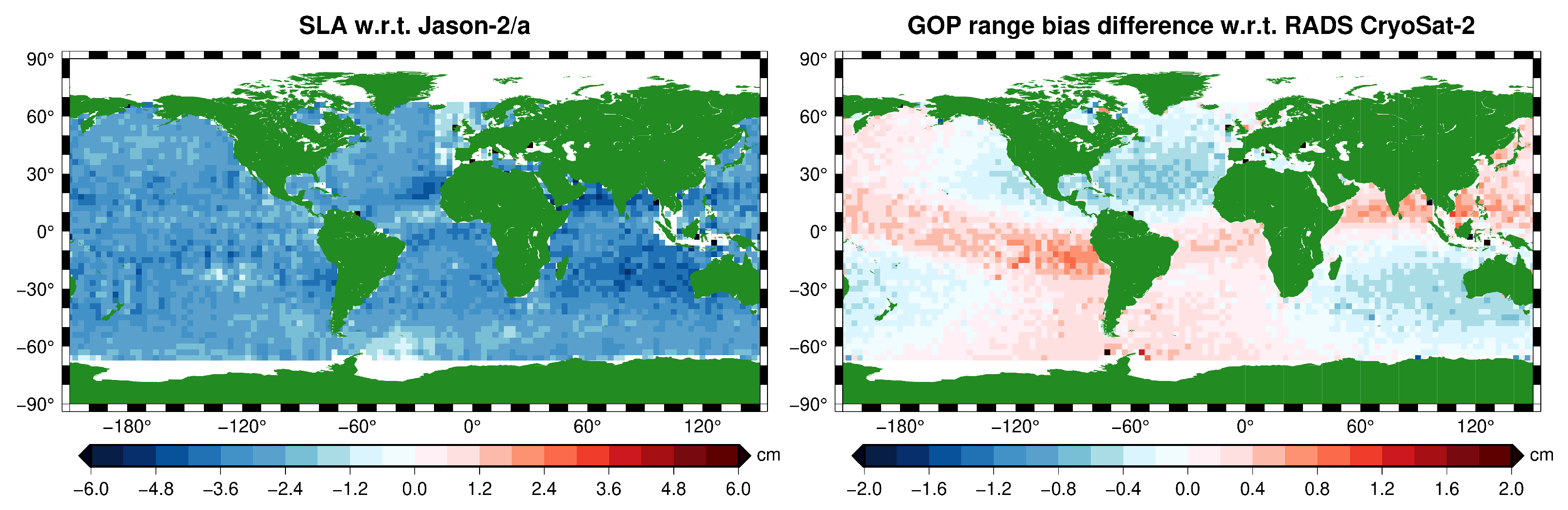
rforeference frame offsetresult from cal/val activities (−2.9 cm for RADS CryoSat-2)
Table 4. Satellite crossover statistics with mean and standard deviation for SLA, SWH, σ 0 , wind speed (WIND), and sea state bias (SSB). Crossovers with | Δ t | > 2 days, beneath 70 and above + 70 latitude, and larger than 2 times the standard deviation of the XO differences per pass, were rejected. The last column displays the number of XOs surviving these edit criteria.
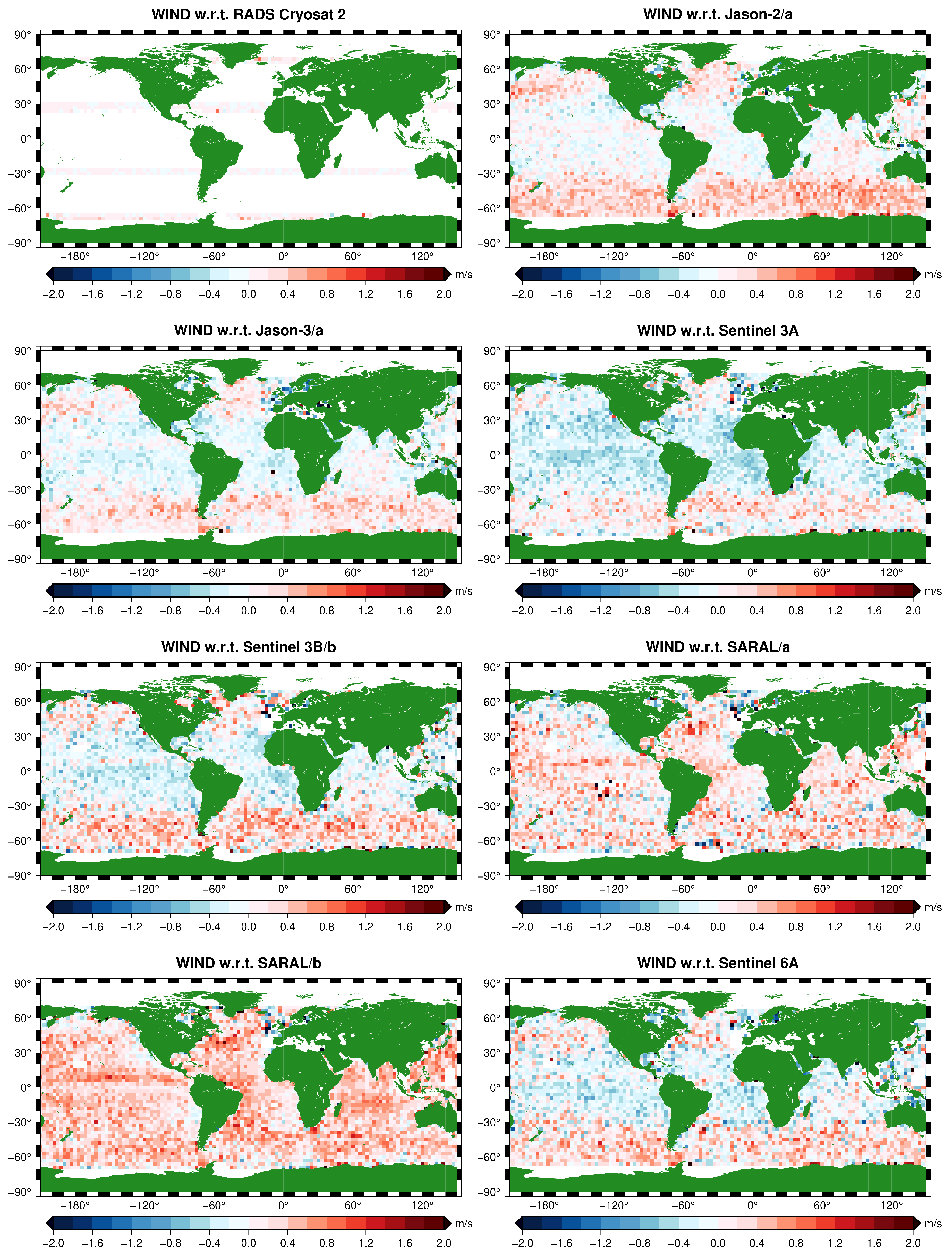
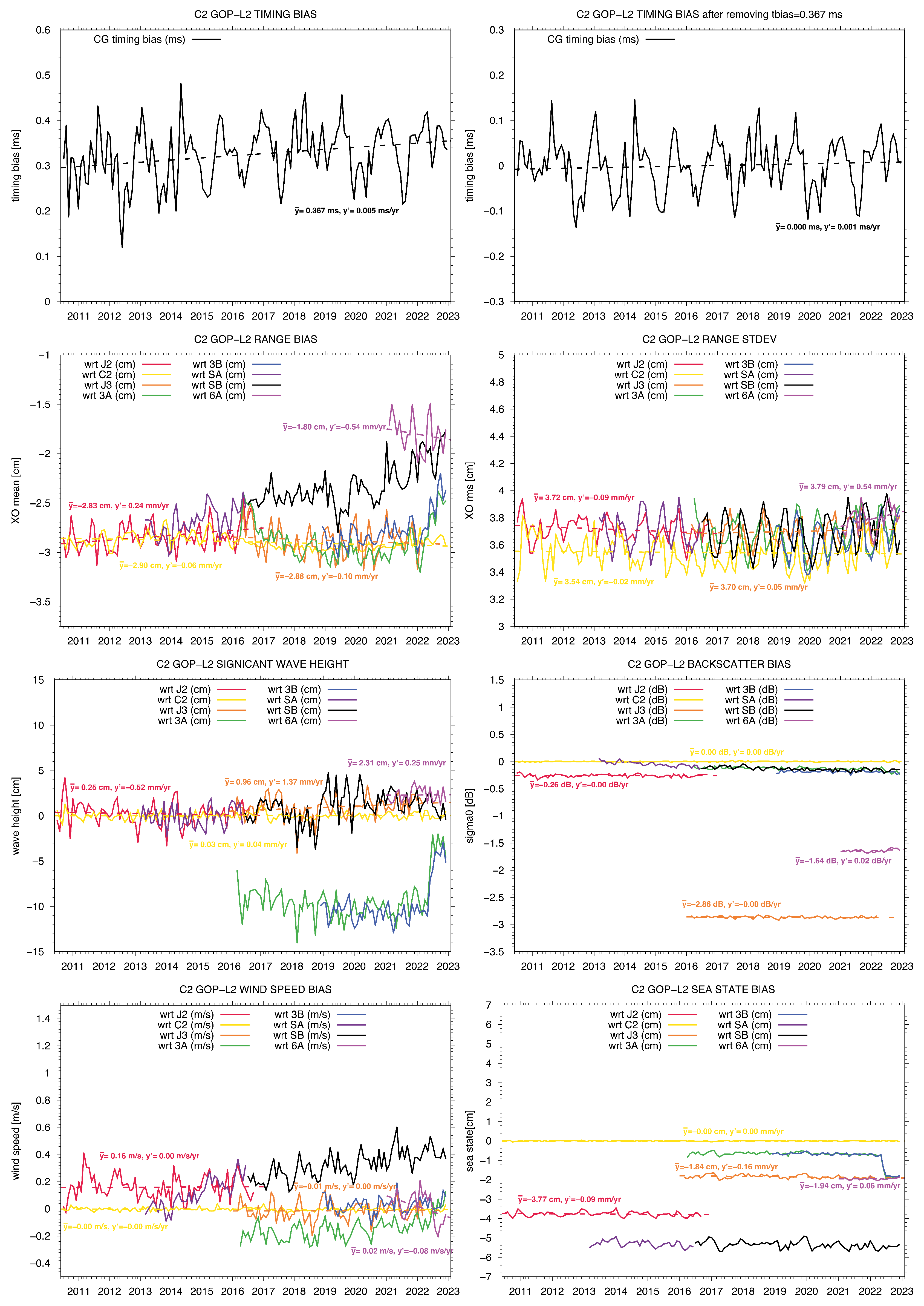
(a) Dual-satellite crossover statistics for GOP CryoSat-2 crossings with RADS CryoSat-2, Jason-2, Jason-3, Sentinel-3A, Sentinel-3BSARAL, and Sentinel-6A. The last row displays the average of the SLA mean and rms difference in the satellite phases that are the longest, leaving out SARAL (other altimeter type) and leaving out Sentinel-6A (too much of a deviating XO mean).
with respect toSLA [m]SWH [m] σ 0 [dB]WIND [m/s]SSB [m]XOs [no.]
meansdmeansdmeansdmeansdmeansd
C2−0.0290.0350.0000.7100.0011.585−0.0032.770−0.0000.032343,365
J2a−0.0290.0370.0021.006−0.2571.4510.1673.521−0.0380.0381,133,727
J2b−0.0280.0360.0080.998−0.2491.4850.1433.545−0.0370.038116,963
J2c−0.0290.0370.0011.006−0.2321.4870.0733.593−0.0380.038177,958
J2d−0.0290.0370.0081.008−0.2541.4900.1243.520−0.0380.038160,395
J3a−0.0290.0370.0101.015−2.8631.521−0.0113.605−0.0180.0381,286,827
J3b−0.0260.0390.0211.021−2.8501.500−0.0643.563−0.0190.038135,512
3A−0.0290.037−0.0930.952−0.1281.517−0.1483.275−0.0080.036620,735
3Ba−0.0330.039−0.0760.957−0.1731.547−0.0513.199−0.0070.03631,053
3Bb−0.0280.037−0.0990.953−0.1871.5130.0323.238−0.0080.036375,064
SAa−0.0270.037−0.0020.945−0.0431.6340.1153.175−0.0530.037288,403
SAb−0.0230.0370.0100.936−0.1311.6350.3233.146−0.0540.037529,370
6A−0.0180.0380.0231.017−1.6411.4840.0193.574−0.0190.038428,821
avg 0.029 0.037 ---------
(b) Single-satellite crossover statistics for GOP CryoSat-2, RADS CryoSat-2, Jason-2, Jason-3, Sentinel-3A, Sentinel-3B, and Sentinel-6A.
SLA [m]SWH [m] σ 0 [dB]WIND [m/s]SSB [m]XOs [no.]
meansdmeansdmeansdmeansdmeansd
CG−0.0070.035−0.0000.715−0.0051.591−0.0132.7880.0000.032179,905
C2−0.0070.0350.0020.710−0.0031.586−0.0142.7650.0000.032128,201
J2a−0.0000.034−0.0030.9810.0031.440−0.0063.4400.0000.032522,648
J2b0.0000.033−0.0010.9780.0031.470−0.0023.4820.0000.03251,426
J2c0.0010.034−0.0040.983−0.0081.4640.0183.5110.0000.03280,525
J2d0.0010.0350.0040.9820.0081.490−0.0103.448−0.0000.03171,546
J3a0.0000.0350.0011.0060.0041.571−0.0033.6230.0000.034608,933
J3b0.0000.0380.0021.003−0.0031.5530.0143.632−0.0000.03474,187
3A0.0030.034−0.0080.9580.0151.636−0.0213.2190.0000.032340,851
3Ba0.0010.034−0.0090.9270.0121.700−0.0243.0510.0000.03016,685
3Bb0.0030.034−0.0010.9570.0151.617−0.0193.1530.0000.032208,379
SAa0.0020.0330.0010.930−0.0121.7700.0342.948−0.0000.022158,932
SAb0.0030.0340.0030.919−0.0051.7570.0262.901−0.0000.022276,546
6A0.0000.0350.0011.0080.0011.5340.0073.605−0.0000.034210,622
Table 5. Summary of GOP CryoSat-2 (CG) and Jason-2–Jason-3 (REF) comparison with PSMSL tide gauges (TG) for 309 selected tide gauge stations during the period from 2010 up to and including 2021.
Correlation [-]St. Dev. [cm]Tilt [mm/yr]
CG −TG0.825.70.17
REF − TG0.844.9−0.11
mean GIA −0.27
Disclaimer/Publisher’s Note: The statements, opinions and data contained in all publications are solely those of the individual author(s) and contributor(s) and not of MDPI and/or the editor(s). MDPI and/or the editor(s) disclaim responsibility for any injury to people or property resulting from any ideas, methods, instructions or products referred to in the content.

