
Utility of Leaf Area Index for Monitoring Phenology of Russian Forests

 ,
,
Abstract
:1. Introduction
2. Materials and Methods
2.1. IKI MODIS NDVI, EVI2, FPAR, and LAI Products
2.2. NASA MODIS MCD12Q2 Phenology Product
2.3. Empirical and Theoretical Background on Seasonal Variation in NDVI, EVI2, and LAI
2.4. Retrievals of Phenometrics from the Seasonal LAI Profiles
3. Results
3.1. MODIS Data Coverage Limitations
3.2. Comparison of Dynamic Properties of NDVI, EVI2, FPAR and LAI
3.3. Analysis of Retrieved Phenometrics
3.4. Sensitivity Analysis
4. Conclusions
Supplementary Materials
Author Contributions
Funding
Data Availability Statement
Acknowledgments
Conflicts of Interest
Appendix A. IKI MODIS Forest Species Product

Appendix B. Striping Artefacts in MODIS Channel Data

References
- Moon, M.; Li, D.; Liao, W.; Rigden, A.J.; Friedl, M.A. Modification of surface energy balance during springtime: The relative importance of biophysical and meteorological changes. Agric. For. Meteorol. 2020, 284, 107905. [Google Scholar] [CrossRef]
- Richardson, A.D.; Keenan, T.F.; Migliavacca, M.; Ryu, Y.; Sonnentag, O.; Toomey, M. Climate change, phenology, and phenological control of vegetation feedbacks to the climate system. Agric. For. Meteorol. 2013, 169, 156–173. [Google Scholar] [CrossRef]
- Møller, A.P.; Rubolini, D.; Lehikoinen, E. Populations of migratory bird species that did not show a phenological response to climate change are declining. Proc. Natl. Acad. Sci. USA 2008, 105, 16195–16200. [Google Scholar] [CrossRef] [PubMed]
- Zhu, Z.; Woodcock, C.E. Continuous change detection and classification of land cover using all available Landsat data. Remote Sens. Environ. 2014, 144, 152–171. [Google Scholar] [CrossRef]
- Bolton, D.K.; Friedl, M.A. Forecasting crop yield using remotely sensed vegetation indices and crop phenology metrics. Agric. For. Meteorol. 2013, 173, 74–84. [Google Scholar] [CrossRef]
- Sacks, W.J.; Deryng, D.; Foley, J.A.; Ramankutty, N. Crop planting dates: An analysis of global patterns. Glob. Ecol. Biogeogr. 2010, 19, 607–620. [Google Scholar] [CrossRef]
- de Beurs, K.M.; Henebry, G.M. Land surface phenology and temperature variation in the International Geosphere-Biosphere Program high-latitude transects. Glob. Chang. Biol. 2005, 11, 779–790. [Google Scholar] [CrossRef]
- Shabanov, N.V.; Marshall, G.J.; Rees, W.G.; Bartalev, S.A.; Tutubalina, O.V.; Golubeva, E.I. Climate-driven phenological changes in the Russian Arctic derived from MODIS LAI time series 2000–2019. Environ. Res. Lett. 2021, 16, 084009. [Google Scholar] [CrossRef]
- Norton, A.J.; Bloom, A.A.; Parazoo, N.C.; Levine, P.A.; Ma, S.; Braghiere, R.K.; Smallman, T.L. Improved process representation of leaf phenology significantly shifts climate sensitivity of ecosystem carbon balance. Biogeosciences 2023, 20, 2455–2484. [Google Scholar] [CrossRef]
- Zhang, J.; Zhao, J.; Wang, Y.; Zhang, H.; Zhang, Z.; Guo, X. Comparison of land surface phenology in the Northern Hemisphere based on AVHRR GIMMS3g and MODIS datasets. ISPRS J. Photogramm. Remote Sens. 2020, 169, 1–16. [Google Scholar] [CrossRef]
- Bornez, K.; Descals, A.; Verger, A.; Peñuelas, J. Land surface phenology from VEGETATION and PROBA-V data. Assessment over deciduous forests. Int. J. Appl. Earth Obs. Geoinf. 2020, 84, 101974. [Google Scholar] [CrossRef]
- Rodriguez-Galiano, V.F.; Dash, J.; Atkinson, P.M. Characterising the Land Surface Phenology of Europe Using Decadal MERIS Data. Remote Sens. 2015, 7, 9390–9409. [Google Scholar] [CrossRef]
- Ganguly, S.; Friedl, M.A.; Tan, B.; Zhang, X.; Verma, M. Land surface phenology from MODIS: Characterization of the Collection 5 global land cover dynamics product. Remote Sens. Environ. 2010, 114, 1805–1816. [Google Scholar] [CrossRef]
- Zhang, X.; Liu, L.; Yan, D. Comparisons of global land surface seasonality and phenology derived from AVHRR, MODIS, and VIIRS data. J. Geophys. Res. Biogeosci. 2017, 122, 1506–1525. [Google Scholar] [CrossRef]
- Bolton, D.K.; Gray, J.M.; Melaas, E.K.; Moon, M.; Eklundh, L.; Friedl, M.A. Continental-scale land surface phenology from harmonized Landsat 8 and Sentinel-2 imagery. Remote Sens. Environ. 2020, 240, 111685. [Google Scholar] [CrossRef]
- Yan, D.; Zhang, X.; Nagai, S.; Yu, Y.; Akitsu, T.; Nasahara, K.N.; Ide, R.; Maeda, T. Evaluating land surface phenology from the Advanced Himawari Imager using observations from MODIS and the Phenological Eyes Network. Int. J. Appl. Earth Obs. Geoinf. 2019, 79, 71–83. [Google Scholar] [CrossRef]
- Yan, K.; Park, T.; Yan, G.; Liu, Z.; Yang, B.; Chen, C.; Nemani, R.R.; Knyazikhin, Y.; Myneni, R.B. Evaluation of MODIS LAI/FPAR Product Collection 6. Part 2: Validation and Intercomparison. Remote Sens. 2016, 8, 460. [Google Scholar] [CrossRef]
- Huang, D.; Knyazikhin, Y.; Wang, W.; Deering, D.W.; Stenberg, P.; Shabanov, N.; Tan, B.; Myneni, R.B. Stochastic Transport Theory for Investigating the Three-Dimensional Canopy Structure from Space Measurements. Remote Sens. Environ. 2008, 112, 35–50. [Google Scholar] [CrossRef]
- Knyazikhin, Y.; Martonchik, J.V.; Myneni, R.B.; Diner, D.J.; Runing, S. Synergistic algorithm for estimating vegetation canopy leaf area index and fraction of absorbed photosynthetically active radiation from MODIS and MISR data. J. Geophys. Res. Atmos. 1998, 103, 32257–32277. [Google Scholar] [CrossRef]
- Myneni, R.B.; Williams, D.L. On the relationship between FAPAR and NDVI. Remote Sens. Environ. 1994, 49, 200–211. [Google Scholar] [CrossRef]
- Wang, S.; Lu, X.; Cheng, X.; Li, X.; Peichl, M.; Mammarella, I. Limitations and challenges of MODIS-derived phenological metrics across different landscapes in pan-Arctic regions. Remote Sens. 2018, 10, 1784. [Google Scholar] [CrossRef]
- Shabanov, N.V.; Bartalev, S.A.; Kobayashi, H.; Shin, N.; Khovratovich, T.S.; Zharko, V.O.; Medvedev, A.A.; Telnova, N.O. A Semiempirical Approach for Decomposition of Remotely Sensed Leaf Area Index into Overstory and Understory Components over Russian Forests. IEEE Trans. Geosci. Remote Sens. 2023, 61, 1–17. [Google Scholar] [CrossRef]
- Jonckheere, I.; Fleck, S.; Nackaerts, K.; Muys, B.; Coppin, P.; Weiss, M.; Baret, F. Review of methods for in situ leaf area index determination Part I. Theories, sensors and hemispherical photography. Remote Sens. Environ. 2004, 121, 19–35. [Google Scholar]
- Shabanov, N.V.; Knyazikhin, Y.; Baret, F.; Myneni, R.B. Stochastic Modeling of Radiation Regime in Discontinuous Vegetation Canopies. Remote Sens. Environ. 2000, 74, 125–144. [Google Scholar] [CrossRef]
- Miklashevich, T.S.; Bartalev, S.A.; Plotnikov, D.E. Interpolation Algorithm for Recovery of Long Satellite Data Time Series of Vegetation Cover Observations. Sovrem. Probl. Distantsionnogo Zondirovaniya Zemli Iz Kosmosa 2019, 16, 143–154. (In Russian) [Google Scholar] [CrossRef]
- Jiang, Z.; Huete, A.; Didan, K.; Miura, T. Development of a two-band enhanced vegetation index without a blue band. Remote Sens. Environ. 2008, 112, 3833–3845. [Google Scholar] [CrossRef]
- Waring, R.H.; Running, S.W. Forest Ecosystems: Analysis at Multiple Scales, 3rd ed.; Elsevier: Burlington, MA, USA; Academic Press: Burlington, MA, USA, 2010; p. 440. [Google Scholar]
- Majasalmi, T.; Rautiainen, M. Potential of using surface temperature data to benchmark Sentinel-2based forest phenometrics in boreal Finland. Ann. For. Sci. 2022, 79, 6. [Google Scholar] [CrossRef]
- Ahl, D.E.; Gower, S.T.; Burrows, S.N.; Shabanov, N.V.; Myneni, R.B.; Knyazikhin, Y. Monitoring Spring Canopy Phenology of a Deciduous Broadleaf Forest using MODIS. Remote Sens. Environ. 2006, 104, 88–95. [Google Scholar] [CrossRef]
- Rautiainen, M.; Mõttus, M.; Heiskanen, J.; Akujärvi, A.; Majasalmi, T.; Stenberg, P. Seasonal reflectance dynamics of common understory types in a Northern European boreal forest. Remote Sens. Environ. 2011, 115, 3020–3028. [Google Scholar] [CrossRef]
- Cohen, W.B.; Maiersperger, T.K.; Turner, D.P.; Ritts, W.D.; Pflugmacher, D.; Kennedy, R.E.; Kirschbaum, A.; Running, S.W.; Costa, M.; Gower, S.T. MODIS land cover and LAICollection 4 product quality across nine sites in the Western Hemisphere. IEEE Trans. Geosci. Remote Sens. 2006, 44, 1843–1857. [Google Scholar] [CrossRef]
- Garrigues, S.; Lacaze, R.; Baret, F.; Morisette, J.T.; Weiss, M.; Nickeson, J.; Fernandes, R.; Plummer, S.; Shabanov, N.V.; Myneni, R.; et al. Validation and Intercomparison of Global Leaf Area Index Products Derived from Remote Sensing Data. J. Geophys. Res. Atmos. 2008, 113, G02028. [Google Scholar] [CrossRef]
- Kobayashi, H.; Delbart, N.; Suzuki, R.; Kushida, K. A satellite based method for monitoring seasonality in the overstory leaf area index of Siberian larch forest. J. Geophys. Res.-Biogeosci. 2010, 115, G01002. [Google Scholar] [CrossRef]
- Loupian, E.A.; Proshin, A.A.; Bourtsev, M.A.; Kashnitskii, A.V.; Balashov, I.V.; Bartalev, S.A.; Konstantinova, A.M.; Kobets, D.A.; Mazurov, A.A.; Marchenkov, V.V.; et al. Experience of development and operation of the IKI-Monitoring center for collective use of systems for archiving, processing and analyzing satellite data. Sovrem. Probl. Distantsionnogo Zondirovaniya Zemli Iz Kosmosa 2019, 16, 151–170. (In Russian) [Google Scholar] [CrossRef]
- Bartalev, S.; Egorov, V.; Zharko, V.; Loupian, E.; Plotnikov, D.; Khvostikov, S.; Shabanov, N. Land Cover Mapping over Russia Using Earth Observation Data; Russian Academy of Sciences’ Space Research Institute: Moscow, Russia, 2016; p. 208. [Google Scholar]
- Bartalev, S.; Egorov, V.; Loupian, E.; Khvostikov, S. A new locally-adaptive classification method LAGMA for large-scale land cover mapping using remote-sensing data. Remote Sens. Lett. 2014, 5, 55–64. [Google Scholar] [CrossRef]
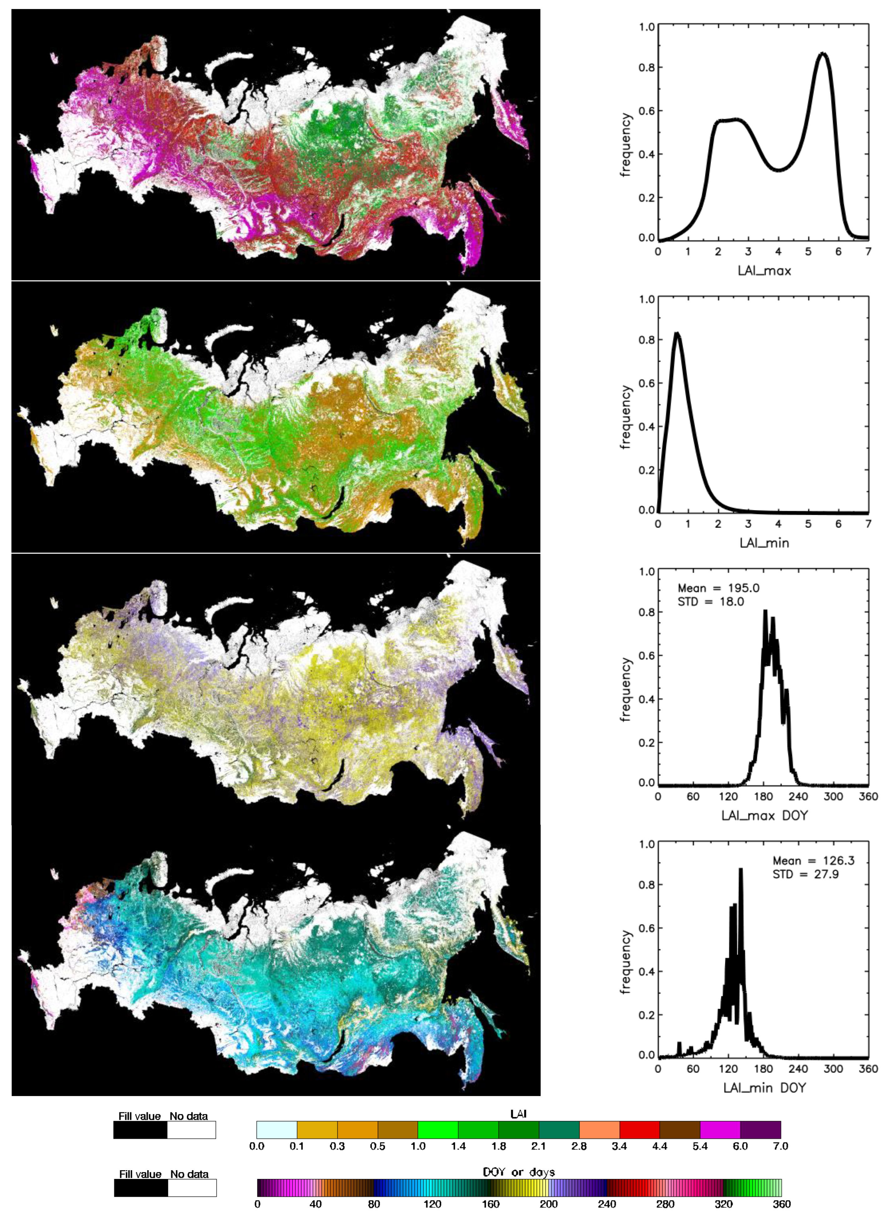
 , 50% over DOYs 157–240 in blue
  , and 15% over DOYs 138–261 in green
  . At the boundaries of brown
  interval DOYs 126–281, LAI reaches minimum in spring and fall. Panel (b) shows latitudinal distribution of annual data availability, the ratio of annual sum of valid LAI pixels to total forest pixels in a given latitudinal band.
, 50% over DOYs 157–240 in blue , and 15% over DOYs 138–261 in green . At the boundaries of brown interval DOYs 126–281, LAI reaches minimum in spring and fall. Panel (b) shows latitudinal distribution of annual data availability, the ratio of annual sum of valid LAI pixels to total forest pixels in a given latitudinal band.
interval DOYs 126–281, LAI reaches minimum in spring and fall. Panel (b) shows latitudinal distribution of annual data availability, the ratio of annual sum of valid LAI pixels to total forest pixels in a given latitudinal band.
, 50% over DOYs 157–240 in blue , and 15% over DOYs 138–261 in green . At the boundaries of brown interval DOYs 126–281, LAI reaches minimum in spring and fall. Panel (b) shows latitudinal distribution of annual data availability, the ratio of annual sum of valid LAI pixels to total forest pixels in a given latitudinal band.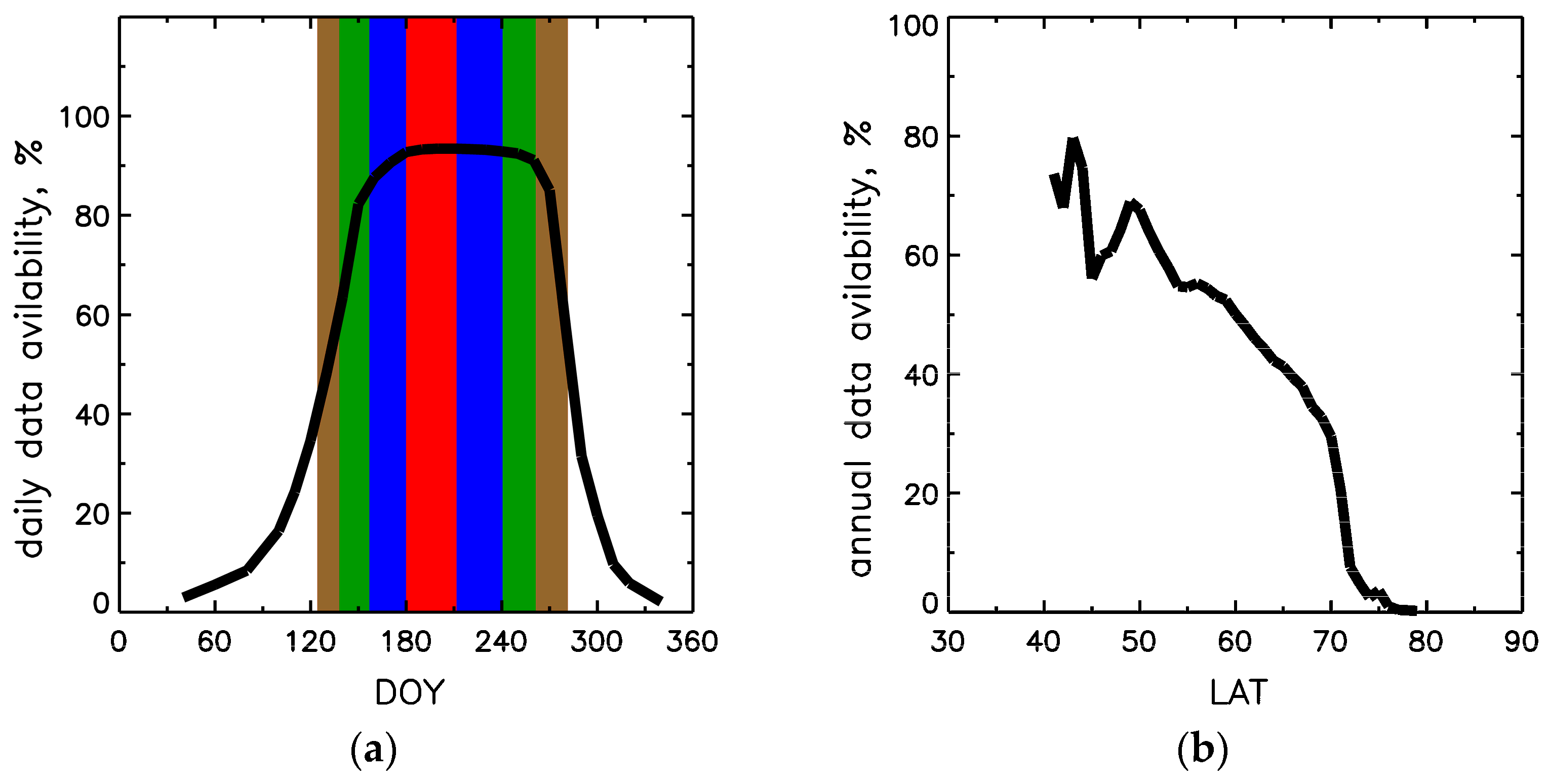


| Phenometrics | Definition |
|---|---|
| greenup | Date when base variable first crosses 15% of amplitude of its variations |
| mid-greening | Date when base variable first crosses 50% of amplitude of its variations |
| maturity | Date when base variable first crosses 90% of amplitude of its variations |
| maximum | Date when seasonal maximum is achieved |
| senescence | Date when base variable last crosses 90% of amplitude of its variations |
| mid-browning | Date when base variable last crosses 50% of amplitude of its variations |
| dormancy | Date when base variable last crosses 15% of amplitude of its variations |
| minimum | Minimum value of the base variable |
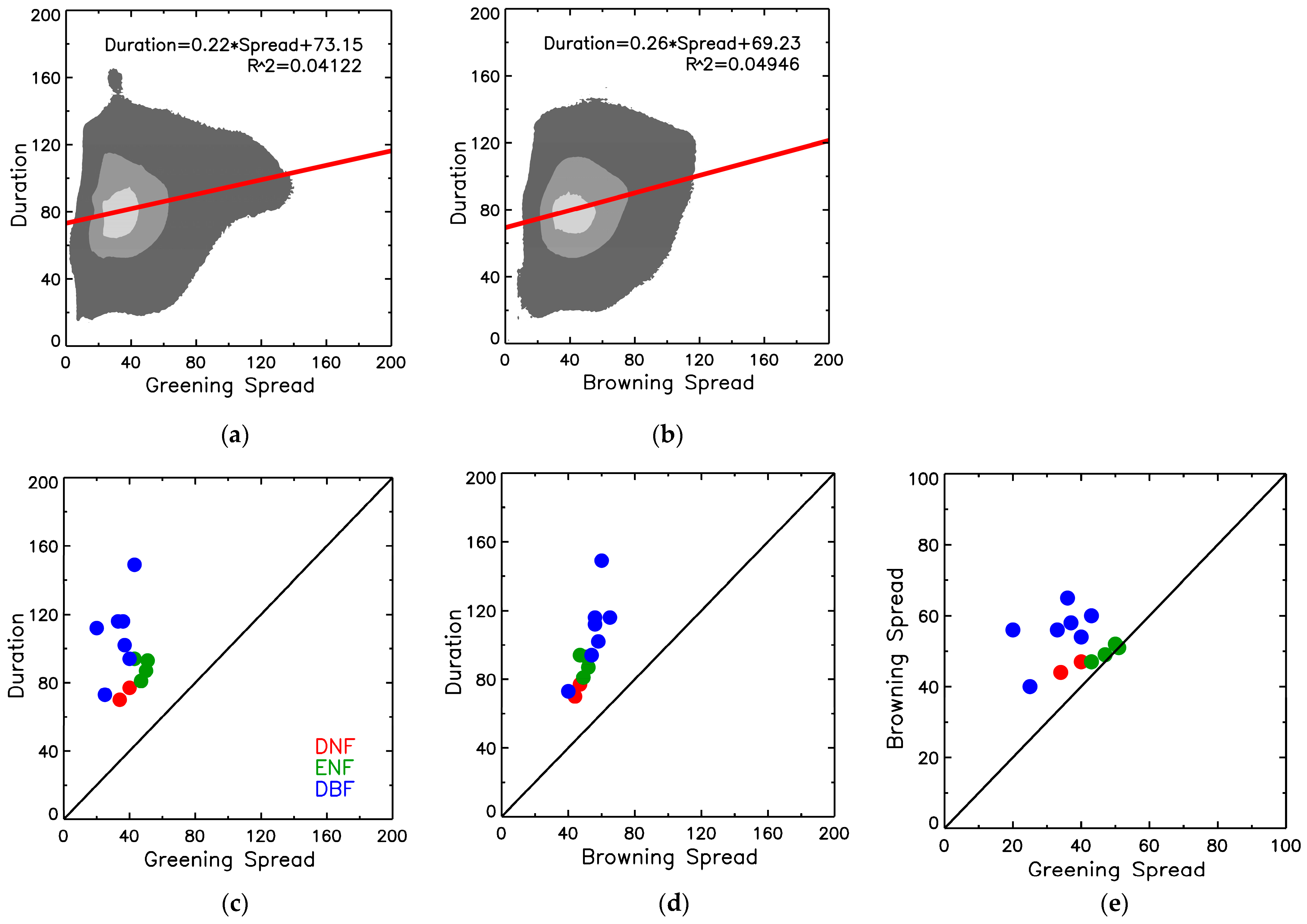
| duration * | Difference between mid-browning and mid-greening dates |
| greening spread * | Difference between maturity and greenup dates |
| browning spread * | Difference between formancy and denescence dates |
| amplitude | Difference between maximum and minimum of base variable |
| integral | Integral of base variable from greenup to dormancy |
| (a) | |||||||||||||||||
|---|---|---|---|---|---|---|---|---|---|---|---|---|---|---|---|---|---|
| Forest Classes | Forest Species | Greening Min LAI | Max LAI | Browning Min LAI | LAI Amplitude | ||||||||||||
| LAI | DOY | LAI | DOY | LAI | DOY | Greening | Browning | ||||||||||
| DNF | Sparse larch | 0.9 | 145 | 2.3 | 195 | 0.5 | 271 | 1.4 | 1.8 | ||||||||
| Larch | 0.8 | 128 | 3.4 | 194 | 0.5 | 279 | 2.6 | 2.9 | |||||||||
| ENF | Pine | 1.1 | 116 | 4.4 | 196 | 0.9 | 282 | 3.3 | 3.5 | ||||||||
| Spruce | 1.2 | 124 | 4.8 | 200 | 1.0 | 279 | 3.6 | 3.8 | |||||||||
| Fir | 1.3 | 118 | 5.0 | 192 | 1.1 | 270 | 3.7 | 3.9 | |||||||||
| Siberian pine | 1.1 | 111 | 4.8 | 196 | 0.9 | 283 | 3.7 | 3.9 | |||||||||
| DBF | Oak | 0.5 | 79 | 5.9 | 183 | 0.4 | 318 | 5.4 | 5.5 | ||||||||
| Beech | 0.6 | 54 | 5.9 | 187 | 0.5 | 331 | 5.3 | 5.4 | |||||||||
| Stone birch | 1.1 | 160 | 5.5 | 207 | 0.5 | 294 | 4.4 | 5.0 | |||||||||
| Birch | 0.6 | 109 | 5.4 | 189 | 0.5 | 287 | 4.8 | 4.9 | |||||||||
| Aspen | 0.6 | 103 | 5.7 | 183 | 0.6 | 288 | 5.1 | 5.1 | |||||||||
| Linden | 0.5 | 104 | 5.9 | 182 | 0.4 | 309 | 5.4 | 5.5 | |||||||||
| Maple | 0.5 | 112 | 5.8 | 172 | 0.4 | 302 | 5.3 | 5.4 | |||||||||
| (b) | |||||||||||||||||
| Forest Classes | Forest Species | Greening dates and spread | Browning dates and spread | Duration days | |||||||||||||
| 15% | 50% | 90% | Spread | 90% | 50% | 15% | Spread | 15% | 50% | 90% | |||||||
| DNF | Sparse larch | 151 | 165 | 185 | 34 | 209 | 235 | 253 | 44 | 102 | 70 | 24 | |||||
| Larch | 141 | 159 | 182 | 41 | 209 | 237 | 256 | 47 | 114 | 78 | 27 | ||||||
| ENF | Pine | 131 | 154 | 181 | 50 | 213 | 242 | 265 | 52 | 133 | 87 | 32 | |||||
| Spruce | 137 | 160 | 185 | 48 | 215 | 242 | 263 | 48 | 126 | 82 | 31 | ||||||
| Fir | 127 | 145 | 171 | 44 | 214 | 241 | 259 | 45 | 132 | 96 | 43 | ||||||
| Siberian pine | 126 | 150 | 178 | 52 | 214 | 243 | 265 | 51 | 139 | 92 | 36 | ||||||
| DBF | Oak | 121 | 138 | 159 | 37 | 212 | 252 | 278 | 66 | 156 | 114 | 53 | |||||
| Beech | 108 | 127 | 150 | 42 | 235 | 276 | 297 | 62 | 188 | 149 | 85 | ||||||
| Stone birch | 166 | 175 | 191 | 25 | 225 | 249 | 266 | 41 | 100 | 74 | 35 | ||||||
| Birch | 129 | 149 | 169 | 40 | 211 | 243 | 265 | 54 | 135 | 94 | 41 | ||||||
| Aspen | 124 | 142 | 162 | 38 | 209 | 243 | 266 | 57 | 142 | 101 | 47 | ||||||
| Linden | 122 | 137 | 156 | 34 | 217 | 254 | 273 | 56 | 151 | 116 | 60 | ||||||
| Maple | 124 | 135 | 150 | 26 | 204 | 239 | 267 | 63 | 143 | 103 | 54 | ||||||
Disclaimer/Publisher’s Note: The statements, opinions and data contained in all publications are solely those of the individual author(s) and contributor(s) and not of MDPI and/or the editor(s). MDPI and/or the editor(s) disclaim responsibility for any injury to people or property resulting from any ideas, methods, instructions or products referred to in the content. |
© 2023 by the authors. Licensee MDPI, Basel, Switzerland. This article is an open access article distributed under the terms and conditions of the Creative Commons Attribution (CC BY) license (https://creativecommons.org/licenses/by/4.0/).
Share and Cite
Shabanov, N.V.; Egorov, V.A.; Miklashevich, T.S.; Stytsenko, E.A.; Bartalev, S.A. Utility of Leaf Area Index for Monitoring Phenology of Russian Forests. Remote Sens. 2023, 15, 5419. https://doi.org/10.3390/rs15225419
Shabanov NV, Egorov VA, Miklashevich TS, Stytsenko EA, Bartalev SA. Utility of Leaf Area Index for Monitoring Phenology of Russian Forests. Remote Sensing. 2023; 15(22):5419. https://doi.org/10.3390/rs15225419
Chicago/Turabian StyleShabanov, Nikolay V., Vyacheslav A. Egorov, Tatiana S. Miklashevich, Ekaterina A. Stytsenko, and Sergey A. Bartalev. 2023. "Utility of Leaf Area Index for Monitoring Phenology of Russian Forests" Remote Sensing 15, no. 22: 5419. https://doi.org/10.3390/rs15225419
APA StyleShabanov, N. V., Egorov, V. A., Miklashevich, T. S., Stytsenko, E. A., & Bartalev, S. A. (2023). Utility of Leaf Area Index for Monitoring Phenology of Russian Forests. Remote Sensing, 15(22), 5419. https://doi.org/10.3390/rs15225419