Machine and Deep Learning Regression of Chlorophyll-a Concentrations in Lakes Using PRISMA Satellite Hyperspectral Imagery

Abstract

The estimation of Chlorophyll-a concentration is crucial for monitoring freshwater ecosystem health, particularly in lakes, as it is closely linked to eutrophication processes. Satellite imagery enables synoptic and frequent evaluations of Chlorophyll-a in water bodies, providing essential insights into spatiotemporal eutrophication dynamics. Frontier applications in water remote sensing support the utilization of machine and deep learning models applied to hyperspectral satellite imagery. This paper presents a comparative analysis of conventional machine and deep learning models—namely, Random Forest Regressor, Support Vector Regressor, Long Short-Term Memory, and Gated Recurrent Unit networks—for estimating Chlorophyll-a concentrations. The analysis is based on data from the PRecursore IperSpettrale della Missione Applicativa (PRISMA) hyperspectral mission, complemented by low-resolution Chlorophyll-a concentration maps. The analysis focuses on three sub-alpine lakes, spanning Northern Italy and Switzerland as testing areas. Through a series of modelling experiments, best-performing model configurations are pinpointed for both Chlorophyll-a concentration estimations and the improvement of spatial resolution in predictions. Support Vector Regressor demonstrated a superior performance in Chlorophyll-a concentration estimations, while Random Forest Regressor emerged as the most effective solution for refining the spatial resolution of predictions.

1. Introduction

Eutrophication is predominantly an anthropogenic process characterized by an excessive accumulation of nutrients, primarily nitrogen and phosphorus, in surface freshwater ecosystems such as lakes. This nutrient excess promotes the rapid growth of algae and aquatic plants which can increase both water turbidity and, as algae die and decompose, water oxygen depletion, leading to negative impacts on aquatic life and lake ecosystems [1]. Human disturbances to the water cycle, such as agricultural runoff, urban development, and wastewater discharge, mostly contribute to eutrophication [2]. Therefore, controlling and mitigating lake eutrophication is essential to protect both freshwater ecosystems and human well-being by maintaining the ecological and economic value of lakes [3]. The need to preserve freshwater ecosystems is further enforced by their direct connection with the United Nations Sustainable Development Goal 6 (SDG 6: Ensure availability and sustainable management of water and sanitation for all) [4]. Accordingly, effective control and mitigation actions towards freshwater ecosystem protection are imperative and require both space- and time-resolved monitoring and quantification of eutrophication levels in surface water bodies [5].

A significant indicator of eutrophication is the concentration of Chlorophyll in water, which is a major component of algae pigments and cyanobacteria and allows for the estimation of algal biomass in water bodies [6]. Specifically, Chlorophyll-a (Chl-a) is mostly used as a proxy for total algal biomass [7]. Chl-a concentration is relatively easy to measure using various techniques, including imaging spectroscopy [8], and both in-situ and remote sensing methods are often applied in the practice [9]. In-situ monitoring generally suffers from limitations in terms of space–time coverage of measurements [10]. Conversely, remote sensing methods, such as satellite multispectral and hyperspectral imagery, allow for the synoptic assessment of Chl-a concentration over the whole water body’s surface and provide repeated measurements over time, which are critical to capturing eutrophication space–time dynamics [11]. Imaging spectroscopy exploits characteristic Chl-a sunlight absorption and reflection patterns at specific wavelengths including green, blue, red, and near-infrared bands [12] to determine its concentration in water. Airborne and spaceborne imagery has been employed since the 1980s for monitoring Chl-a concentration, proving to be more successful in ocean and seawater applications rather than inland waters due mainly to the limited spatial and spectral resolution of data available at that time [10]. Moreover, the optical complexity of inland waters, primarily caused by a high presence of suspended particles, reduces the reliability of both atmospheric corrections and estimation models initially designed for land and ocean applications [12]. Nonetheless, the detailed and frequent retrieval of inland water biochemical parameters, including Chl-a, has become possible thanks to the latest generation of medium to high spatial resolution multispectral spaceborne sensors, such as those onboard Landsat-8/9, Sentinel-2, and Sentinel-3 satellites [13].

Frontier applications of inland water quality remote monitoring involve hyperspectral satellite imagery, on which bio-optical algorithms demonstrated improved performances compared with multispectral imagery [14,15]. These applications are also favoured by new advancements in global hyperspectral remote sensing, proven by the recent or upcoming launches of hyperspectral satellites [16]. An early example of the above is the Hyperion imager, launched by the United States (US) National Aeronautics and Space Administration (NASA) in 2000 and operational until 2017 [17]. Relevant examples of the most recent missions that provide publicly available imagery are as follows: the German Aerospace Center Earth Sensing Imaging Spectrometer (DESIS) [18] and the hyperspectral imager aboard the Environmental Mapping and Analysis Program (EnMAP) satellite mission [19], the Chinese Advanced Hyperspectral Imager (AHSI) aboard the GaoFeng-5 satellite [20], followed by the launch of the PRecursore IperSpettrale della Missione Applicative (PRISMA) sensor by the Italian Space Agency (ASI) [21], and HyperScout instruments launched on nanosatellites by the European Space Agency (ESA) [22]. These imaging systems offer data cubes where each pixel is composed of several spectral bands enabling space, time and spectral resolved detection of water biochemical constituents [23].

As the resolution and coverage of satellite hyperspectral images continue to improve, cutting-edge data technologies, particularly the implementation of machine and deep learning algorithms [24], are playing a pivotal role in advancing the diffusion and enhancing the capabilities of Chl-a estimation models. Alongside traditional spectral indices and physics-based models [25], machine and deep learning approaches have been frequently exploited in the literature within hyperspectral imaging for Chl-a and other biochemical constituents estimation in water bodies [26]. Recent and pertinent examples are as follows. In [27], Partial Least Squares (PLS) is utilized to determine Chl-a and Total Suspended Matter (TSM). Ref. [28] models in-situ measurements using linear models and Support Vector Machines (SVM) to predict Chl-a concentrations in Lake Taihu (China). Ref. [29] estimates water quality parameters, including Chl-a, for the Elbe River using ten different machine-learning regression models. Ref. [30] evaluates Random Forest (RF), SVM, and Artificial Neural Networks (ANN) for predicting Chl-a concentrations in various inland water bodies, also exploring the inclusion of spectral derivatives as input data. Ref. [31] developed a PLS-ANN model for Chl-a prediction in Lake Erie. Additionally, Ref. [32] utilizes simulated hyperspectral satellite data to predict Chl-a concentrations in lakes, employing an array of models including RF, SVM, Multivariate Adaptive Regression Spline (MARS), and CNN. Ref. [33] generates synthetic EnMAP hyperspectral imagery using EnMAP end-to-end simulator software (EeteS) [34] for Chl-a prediction in Czech Republic water reservoirs using Principal Component Regression, PLS Regression, and RF models. Finally, Refs. [35,36] utilize hyperspectral data from the Hyperspectral Imager for the Coastal Ocean (HICO) [37] and the PRISMA satellite, respectively, to predict Chl-a concentrations using Mixture Density Network (MDN) models.

Despite the availability of machine and deep learning algorithms, there are persistent challenges in implementing them for operational monitoring tasks, often due to a lack of the space–time resolved reference data necessary to train and validate such models [25,38]. With this in mind, the present study aims to employ a variety of machine and deep learning regression models and subsequently conduct a comparative assessment across diverse experimental setups, with the goal of predicting Chl-a concentration maps from medium-resolution hyperspectral satellite imagery through the training and evaluation of these models with reference data characterized by lower spatial resolution, heightened acquisition frequency up to 2 days, and a wide swath width. The objective of the analysis is twofold. Firstly, it aims to verify that the use of the rich spectral information of hyperspectral imagery, coupled with machine and deep learning models, is suitable for reconstructing Chl-a concentration maps using pre-existing and widely accessible reference data. Secondly, it aims to assess the potential for enhancing the spatial resolution of pre-existing Chl-a concentration maps by aligning it with the hyperspectral imagery employed as the regressor in model implementation.

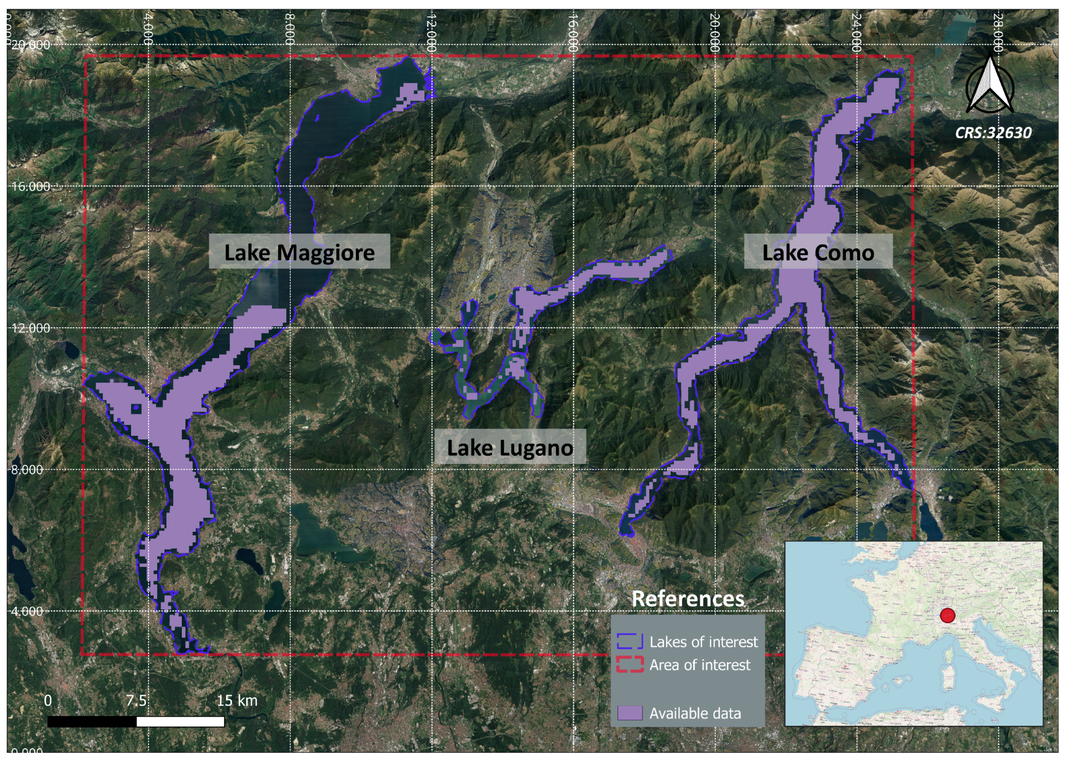
The selected study area includes three sub-alpine lakes between Northern Italy and Switzerland, specifically Lake Como, Lake Maggiore, and Lake Lugano (see Figure 1). These lakes were chosen because they align with the selection made by the “Informative System for the Integrated Monitoring of Insubric Lakes and their Ecosystems” (SIMILE) project, within which this research is conducted. The SIMILE project is funded by the Interreg program of the European Union, which primarily focuses on enhancing coordinated management and stakeholder involvement in monitoring the water quality of sub-alpine lakes between Northern Italy and Switzerland [39,40]. It exploits a combination of in-situ measurements and remote sensing techniques to fulfil its objectives. Within the realm of satellite remote sensing, the project computes three key indicators for assessing lake water quality: Lake Water Surface Temperature derived from Landsat 8 imagery, Total Suspended Matter, and Chl-a concentrations [41] derived from the Sentinel-3 A/B Ocean and Land Colour Instrument (OLCI) imagery at 300 m resolution, which provides a revisit time of less than 2 days. Each of these indicators is monitored by generating time-series of raster maps [42].

In this study, hyperspectral images obtained from the PRISMA mission are used. PRISMA imagery features 239 bands spanning the Visible and Near-Infrared (VNIR) and Short-Wave Infrared (SWIR) regions of the electromagnetic spectrum (400–2500 nm) [21]. PRISMA images have a spatial resolution of 30 m, a Spectral Sampling Interval (SSI) of 12 nm, and a revisit time of 29 days [21]. For model training and testing, time-series maps of Chl-a concentration generated by the SIMILE project team from Sentinel-3 data are employed as low-resolution reference data. Quality assessment for these maps was provided by [40] through comparisons with in-situ measurements, supporting their use as reference Chl-a concentration data in this work. The study considers both machine learning models, such as RF Regressor and SVR, as well as deep learning models such as Long Short-Term Memory (LSTM) networks [43,44] and Gated Recurrent Unit (GRU) networks [45]. The choice of these models is based on empirical evidence from the literature and is primarily guided by two key characteristics, as suggested by [24] and summarized as follows. First, when considering RF Regressor and SVR models, their effectiveness in handling non-linear dependencies within the input data is a primary factor. Moreover, when integrated with dimensionality reduction techniques, these models excel in reducing redundant spectral information. Second, LSTM and GRU models are preferred for their suitability in dealing with hyperspectral imagery. This preference is rooted in the sequential nature of the hyperspectral data, enabling them to capture both long and short-range dependencies of the contiguous bands in the spectral dimension.

The models are employed to (i) reconstruct reference Chl-a concentrations maps computed from Sentinel-3 data, and (ii) augment the spatial resolution of such maps from 300 m to 30 m, thereby aligning them with the resolution of PRISMA imagery. The ultimate goal of such applications is to evaluate the performance of different models in reconstructing the reference Chl-a maps exploiting PRISMA images. Several experiments involving different configurations of model hyperparameters and resolutions for the training/testing datasets were conducted. The resulting accuracies were analyzed statistically to delineate and recommend the most effective models and experimental settings. The SVR model performed best for reconstructing reference Chl-a maps at 300 m spatial resolution, while the RF Regressor model proved to be the most effective for predicting Chl-a maps at 30 m spatial resolution.

The remainder of the paper is as follows. Section 2 describes the data utilized in the study, detailing the criteria for dataset selection, outlining data preparation techniques, and introducing the models considered along with their respective hyperparameter settings. Section 3 presents the outcomes of the modelling experiments, offering a discussion of the significant findings compared with the experimental settings adopted. Finally, Section 4 includes conclusions and future directions of the work.

2. Data and Methods

2.1. Data Procurement and Preprocessing

This study examined two input datasets, namely reference Chl-a concentration raster maps (generated by the SIMILE project at a spatial resolution of 300 m and co-registered on a common grid) and PRISMA hyperspectral imagery with a resolution of 30 m. PRISMA Level L2D geocoded and bottom-of-atmosphere reflectance data [46] were employed in the analysis. The complete time series of reference Chl-a concentration maps encompasses a total of 389 layers, each providing complete coverage of the designated Area of Interest (AOI) within this study (see Figure 1). This time series spans from 15 January 2019 to 5 November 2022. Through the examination of the accessible hyperspectral PRISMA images catalogued in the official missions data portal (http://prisma.asi.it/js-cat-client-prisma-src (accessed on 22 May 2023)), 27 acquisitions that intersected with the AOI in the timeframe of the reference Chl-a maps time series were identified. All bands of each considered PRISMA image were manipulated in the preprocessing operations. Following an initial manual screening process based on the extent of intersection with the reference Chl-a maps, cloud coverage within each PRISMA acquisition, and sun glint disturbance, a total of 12 PRISMA images were deemed suitable. The chosen PRISMA image tiles provided only partial coverage of the AOI, as illustrated in Figure 1. Notably, part of Lake Maggiore is excluded from the analysis due to the unavailability of PRISMA tiles in the catalogue covering that area.

Table 1. Selected pairs of Chl-a maps and PRISMA images with acquisition dates and lakes’ coverage. ID acquisitions are sorted by dates and refer to the original 27 PRISMA acquisitions available in the official mission data portal. Missing IDs correspond to acquisitions excluded after the manual screening.

ID Acquisition	PRISMA Acquisition Date	Lake Como	Lake Maggiore	Lake Lugano	Reference Chl-a Map Date
1	24 April 2020	YES	NO	YES	23 April 2020
2	24 April 2020	YES	NO	NO	23 April 2020
4	25 April 2020	NO	YES	NO	23 April 2020
6	3 July 2020	NO	YES	NO	5 July 2020
10	9 July 2021	YES	NO	YES	9 July 2021
13	31 August 2021	YES	NO	NO	31 August 2021
17	16 October 2021	NO	YES	NO	16 October 2021
18	22 October 2021	YES	NO	NO	22 October 2021
19	22 October 2021	YES	NO	YES	22 October 2021
21	26 November 2021	NO	NO	YES	24 November 2021
23	9 February 2022	NO	YES	NO	9 February 2022
24	27 March 2022	YES	NO	NO	25 March 2022

provides an overview of the dataset utilized in this study. While the acquisition dates of the reference Chl-a maps and the corresponding PRISMA images do not coincide, the maximum temporal discrepancy is limited to 2 days. The table also includes information about the lakes covered by each PRISMA acquisition.

Figure 1 additionally provides a synopsis of the regions containing accessible data, defined as pixels incorporating information on each pair of Chl-a concentration maps and corresponding PRISMA acquisitions across the entirety of the dataset. This pertains to the three lakes within the AOI.

Following the acquisition of PRISMA images, an array of preprocessing operations was executed. This included co-registration, intersection with their reference Chl-a maps, and the removal of null values and anomalous pixels possibly affected by disturbances in water surface spectral signature. The schematic representation of these pre-processing steps is depicted in Figure 2.

While the L2D PRISMA imagery used in this study is already geocoded, an extra step of co-registration was necessary to rectify both local and global distortions. For this purpose, the Python library Gefolki [47] was employed. The co-registration process was critical to ensure accurate alignment of the PRISMA images with the reference data.

The co-registration algorithm implemented in Gefolki computes pixel-wise displacements (optical flow) between pairs of images. A reference grid from the Sentinel-2 mission was considered because of its higher spatial resolution (10 m) and positional accuracy than the original PRISMA grid. To accomplish this, a mosaic using Sentinel-2 images from the period of 11 September 2022 to 18 September 2022 covering the entire AOI was employed. The full AOI coverage could not be achieved with a single Sentinel-2 image tile. Each PRISMA image was resampled to 10 m spatial resolution to perform the co-registration with the Sentinel-2 reference image. The Sentinel-2 mosaic was cropped to the intersected area with the associated PRISMA image, and the displacements between the pixels of the PRISMA image and the reference image were estimated and used to correct the original distortions. Finally, the PRISMA images were resampled to their original resolution (30 m). This procedure is used to co-register all the PRISMA images on a common grid in the final dataset.

After completing the co-registration of the PRISMA images, the next step involved intersecting the co-registered images with their corresponding Chl-a maps. This process aimed to preserve the overlapping regions shared by each acquisition pair. During this operation, pixels with no data in the PRISMA image were set to null in the corresponding Chl-a map, and conversely, for all the acquisition pairs.

The final pre-processing step involved removing anomalous pixels which contained values in the spectral signature inconsistent with the Chl-a concentration recorded in the Chl-a concentration maps, or pixels possibly associated with disturbances on the water surface, such as scum or foam. Anomalous pixels were removed from both the PRISMA images and the corresponding Chl-a maps. To detect the anomalous pixels, the procedure adopted in this study consisted of determining different spectral indices by using the reflectance values of the Sentinel 3 A/B OLCI images that generated the Chl-a maps. These indices are based on bands algebra and were retrieved from the literature with no name associated. The indices were then used to verify the following conditions and identify the anomalous pixel values as shown in Figure 3.

The first condition implies assessing whether, for each pixel, its corresponding value of the Index 1 [48], which is computed using Equation (1), is less than one while the associated Chl-a value exceeds 10 µg/L. Under these circumstances, the pixel is considered anomalous. This is attributed to the expectation that pixels with an index less than one are more likely associated with very low Chl-a concentrations, and conversely.

$$\mathrm{Index}1=\frac{\mathrm{Band}11(708\mathrm{nm})}{\mathrm{Band}8(665\mathrm{nm})}.$$

(1)

It is important to specify that in Equation (1), band 11 of Sentinel-3 A/B OLCI corresponds to the red edge transition of the Chlorophyll fluorescence baseline, while band 8 is linked to the second peak of Chlorophyll absorption [49]. A second condition is used instead to check whether the subsequent ratio [50], computed using Equation (2) and referred to in this work as Index 2, is higher than one for a specific pixel. If so, that pixel should be removed as it may indicate an anomaly on the water surface, likely associated with noise, scum, or foam.

$$\mathrm{Index}2=\frac{\mathrm{Band}12(753\mathrm{nm})}{\mathrm{Band}11(708\mathrm{nm})}.$$

(2)

In Equation (2), band 12 of Sentinel-3 A/B OLCI is used because of its connection to the absorption of oxygen, as well as the presence of clouds and vegetation [49]. The last condition is verified by comparing two indices which are computed using Equations (3) and (4), and referred to in this work respectively as Index 3a and Index 3b. Where one of them is above 1 but the other is not, the pixel is considered anomalous [51]. If both indices are below one, this means that the pixel refers to an area of deep blue water and if the two indices are above one, it is likely that the pixel is related to the presence of phytoplankton.

$$\mathrm{Index}3\mathrm{a}=\frac{\mathrm{Band}6(560\mathrm{nm})}{\mathrm{Band}3(442.5\mathrm{nm})}$$

(3)

$$\mathrm{Index}3\mathrm{b}=\frac{\mathrm{Band}6(560\mathrm{nm})}{\mathrm{Band}4(490\mathrm{nm})}.$$

(4)

In Equations (3) and (4), band 3 of Sentinel-3 A/B OLCI corresponds to the point where Chlorophyll absorption is at its highest, while band 4 indicates areas with high Chlorophyll concentration. Band 6 serves instead as a reference indicator for the lowest Chlorophyll concentration in the image [49].

2.2. Training and Test Datasets Preparation

Following the pre-processing of reference Chl-a maps, it became necessary to devise a data-splitting strategy for the three primary phases involved in the implementation of machine and deep learning models: training (train set), validation (validation set), and evaluation (test set). To accomplish this, an iterative methodology was adopted to uphold consistent distributions between the test set and the combined training and validation set. By allocating pairs of acquisitions to one of the two alternate groups, the distribution of Chl-a values for each group was assessed. The aim was to achieve the most accurate fit to the identity function. To this end, a Quantile-Quantile plot (QQ-plot) was employed (see Figure 4), yielding an $R^2$ of 0.876, thus indicating a robust alignment with the target function. As a result of this process, acquisitions 4, 23, and 24 (see Table 1) were assigned to the test set while the remaining ones were preserved for the training and validation set. Subsequently, the training-validation set was partitioned using a fixed ratio of 80% for training and 20% for validation. Considering the distribution of Chl-a concentrations in the whole dataset, the acquisitions in the test set embed a broad range of Chl-a concentrations. Specifically, acquisition 4 is associated with relatively low-to-medium Chl-a concentrations (mean equal to 3.07 µg/L and a maximum equal to 4.49 µg/L). Acquisitions 23 and 24 depict medium to high Chl-a concentrations, with respective mean concentrations of 5.21 µg/L and 5.21 µg/L, and maximum concentrations of 8.92 µg/L and 7.06 µg/L. This choice was adopted to mitigate possible model over-fitting due to the low number of acquisitions for the study area in the considered time period and to evaluate models on the widest available array of Chl-a concentration episodes. Because of data availability, very high or low Chl-a concentrations could not be included in the test set.

2.3. PRISMA Images Normalization and Dimensionality Reduction

Further operations were conducted on PRISMA images, including normalization and dimensionality reduction. The PRISMA images were initially transformed from their original Digital Number (DN) units to reflectance values, employing the standard formula (see Equation (5)) outlined in the PRISMA data manual [52].

$$x_{scaled}=L2scaleX{X}_{min}+x_{DN}\frac{(L2scaleX{X}_{max}-L2scaleX{X}_{min})}{65.535}.$$

(5)

The term “XX” in Equation (5) denotes a particular region within the input spectrum, either “VNIR” or “SWIR”. L2scale min and max represent the minimum and maximum scaling factors provided in the metadata for each PRISMA image. The normalization value of 65.535 is derived from the computation of $2^{16}-1$, which accounts for the 16-bit coding used to store pixel information. Then, these reflectance values were scaled to a range of [0–$2^{16}$] to store them as unsigned integers (uint16). Starting with this information, three alternative approaches for normalizing the PRISMA images were considered: (i) Min-max scaling, (ii) standard scaling, and (iii) normalization to float reflectance units within the range [0–1], i.e., dividing by the fixed factor of $2^{16}$. Another assessed aspect was the dimensionality reduction of the hyperspectral images. For this purpose, the Principal Component Analysis (PCA) technique was exploited to reduce the spectral dimension to 30 Principal Components (PCs). Finally, the benefits of reducing the spatial dimension were explored by lowering the resolution of the PRISMA images to match that of the associated Chl-a maps, i.e., from 30 m to 300 m. For this case study, the use of 30 PCs explained more than 99% of the variance for all the acquisitions. This was considered sufficient for testing purposes and used as a sample case in the modelling experiments. Different normalization and dimensionality reduction approaches were tested within different modelling experiments, as explained in the following section.

2.4. Machine and Deep Learning Regression Models for Chl-a Concentration

Performances of two machine learning (RF Regressor and SVR) and two deep learning (LSTM and GRU) models in estimating Chl-a concentrations maps by combining Sentinel-3 derived data and PRISMA hyperspectral imagery were explored. The evaluation encompasses a range of hyperparameter settings to identify the most effective combination. Several experiments were designed for each model by intervening in one or more settings. Details are provided in Section 3. The general settings used to define the modelling experiments are outlined below.

• Normalization approach: A set of experiments was conducted to determine the best normalization approach among the ones discussed in Section 2.3.
• Spectral dimensionality reduction: An experiment was conducted to investigate whether the PCA technique contributes or not to the model performances.
• Data augmentation: For the machine learning models, additional bands extracted using image filters were included in the processing. The considered filters were the Sobel X and Sobel Y filters [53], and the Mean filter [54].
• Model hyperparameters: Different hyperparameter settings were investigated for each model following a grid search strategy. The considered hyperparameters are listed in Table 2, Table 3 and Table 4.
• Tests on best input spatial resolution: First, all experiments used 300 m spatial resolution inputs and then, considering the best experiment for each model typology, it was repeated using inputs at 30 m resolution to determine which of the two approaches performed better. This approach was followed because, despite the different spatial resolution, the data derives from the same original distribution, ensuring that the model selection step remains unaffected.

The machine learning models considered in this study were the RF Regressor [55] and the SVR [56]. In some of the experiments, where the spatial downsampling of the PRISMA images to the spatial resolution of the associated Chl-a maps was applied, data augmentation approaches were implemented. These approaches involved extracting additional bands from the input images using the Sobel X and Sobel Y filters, and the Mean filter. The extracted bands were stacked into the input data to augment the dataset size, compensating for the reduction induced by spatial downsampling.

For the implementation of the RF Regressor model, the Scikit-learn Python library was used [57]. Model hyperparameters considered for tuning are described in Table 2.

Table 2. RF Regressor hyperparameters [58].

Parameter	Description
Number of estimators	It is the number of decision trees built. Higher values are expected to improve performance while increasing computational time.
Minimum number of samples per leaf	It sets the minimum samples required for a leaf node, reducing over-fitting with higher values.
Maximum depth of each decision tree	It controls model complexity; large values can lead to over-fitting.

Table 2. RF Regressor hyperparameters [58].

Parameter	Description
Number of estimators	It is the number of decision trees built. Higher values are expected to improve performance while increasing computational time.
Minimum number of samples per leaf	It sets the minimum samples required for a leaf node, reducing over-fitting with higher values.
Maximum depth of each decision tree	It controls model complexity; large values can lead to over-fitting.

Table 3. SVR hyperparameters [59].

Parameter	Description
Gamma	Kernel coefficient for the RBF. It governs the shape of the decision boundary. A high value leads to an extended or complex decision boundary, which, if not carefully controlled, may result in over-fitting.
C	It influences the width of the margin and the tolerance for misclassified data points. It is a regularization hyperparameter which enables to balance between training and testing errors.

Table 3. SVR hyperparameters [59].

Parameter	Description
Gamma	Kernel coefficient for the RBF. It governs the shape of the decision boundary. A high value leads to an extended or complex decision boundary, which, if not carefully controlled, may result in over-fitting.
C	It influences the width of the margin and the tolerance for misclassified data points. It is a regularization hyperparameter which enables to balance between training and testing errors.

For the implementation of the SVR model, the Radial Basis Function (RBF) kernel, computed using the Scikit-learn Python library, was used to conduct trials for the empirical definition of the best hyperparameter values, as detailed in Table 3.

Regarding deep learning models, two architectures were considered, namely LSTM [43,44] and GRU [45] networks. Both are recurrent architectures well suited for the sequential structure of the hyperspectral data. The Tsai Python package [60] was used for their implementation. The hyperparameters considered for the definition of the experiments are explained in Table 4 and these are common for both architectures.

Table 4. LSTM and GRU hyperparameters.

Parameter	Description
Number of layers	The number of LSTM or GRU cells stacked on top of each other.
Dropout in the recurrent neural network cells	Effective regularization method that contrast over-fitting by randomly deactivating a portion of neurons [61]. When dealing with recurrent neurons, dropout is specifically applied to the connections between consecutive recurrent hidden cells.
Dropout in the fully connected layer	Proportion of dropout applied to the fully connected layers’ outputs.
Directionality	Both unidirectional and bidirectional networks were investigated. The difference is that bidirectional networks calculate the hidden state at each time step using information from both past and future inputs, whereas unidirectional networks utilize only past inputs in their calculations.
Hidden size	The number of features in the hidden state.

Table 4. LSTM and GRU hyperparameters.

Parameter	Description
Number of layers	The number of LSTM or GRU cells stacked on top of each other.
Dropout in the recurrent neural network cells	Effective regularization method that contrast over-fitting by randomly deactivating a portion of neurons [61]. When dealing with recurrent neurons, dropout is specifically applied to the connections between consecutive recurrent hidden cells.
Dropout in the fully connected layer	Proportion of dropout applied to the fully connected layers’ outputs.
Directionality	Both unidirectional and bidirectional networks were investigated. The difference is that bidirectional networks calculate the hidden state at each time step using information from both past and future inputs, whereas unidirectional networks utilize only past inputs in their calculations.
Hidden size	The number of features in the hidden state.

3. Results and Discussion

This section reports the results of the modelling experiments described in Section 2.4. The predictive performances of the different models under different settings are reported and compared using well-known metrics, such as the Mean Absolute Error (MAE) and the Root Mean Square Error (RMSE). The evaluation is based on the acquisitions from the test set, specifically acquisitions 4, 23, and 24 (see Section 2.2).

3.1. RF Regressor

A total of 12 experiments with different settings were performed using the RF Regressor model. Experimental settings and results are reported in

Table 5. Settings and results of RF Regressor model experiments. MAE and RMSE represent the average score of the metrics from the application of the experiments to each of the acquisitions in the test set.

Exp. ID	Exp. Setting	Res [m]	PCA	Norm.	Data Augm.	N Trees	Min. Leaf	Max. Depth	MAE [µg/L]	RMSE [µg/L]
RF-1	Norm.	300	No	Minmax	No	1000	3	10	0.931	1.112
RF-2	Norm.	300	No	Std.	No	1000	3	10	0.931	1.112
RF-3	Norm.	300	No	Reflect.	No	1000	3	10	0.931	1.112
RF-4	Spec. red.	300	30 PCs	Std.	No	1000	3	10	1.020	1.245
RF-5	Data augm.	300	No	Std.	Yes	1000	3	10	1.106	1.296
RF-6	Model hyperp.	300	No	Std.	No	1000	3	5	1.032	1.192
RF-7	Model hyperp.	300	No	Std.	No	1000	3	20	0.930	1.113
RF-8	Model hyperp.	300	No	Std.	No	100	3	20	0.947	1.128
RF-9	Model hyperp.	300	No	Std.	No	10,000	3	20	0.924	1.107
RF-10	Model hyperp.	300	No	Std.	No	10,000	2	20	0.915	1.099
RF-11	Model hyperp.	300	No	Std.	No	10,000	10	20	0.934	1.114
RF-12	Spatial res.	30	No	Std.	No	1000	2	20	0.986	1.181

Table abbreviations: Experiment ID (Exp. ID), Experiment setting (Exp. Setting), Input resolution (Res), Normalization (Norm.), Data augmentation (Data augm.), Numbers of estimators (N trees), Minimum number of samples per leaf (Min. leaf), Maximum depth of each decision tree (Max. depth), Spectral dimensionality reduction (Spec. red.), Min-max scaling (Minmax), standard scaling (Std.), normalization to float reflectance units within the range [0, 1] (Reflect.), Model hyperparameters (Model hyperp.).

.

Considering the PRISMA image normalization approaches introduced in Section 2.3, three experiments were carried out (RF-1 to RF-3) to establish the best option. The results achieved by the three experiments are identical in terms of predictive performances, suggesting a negligible effect of the normalization approach on the output.

The fourth experiment (RF-4) was used to evaluate the benefits of applying the PCA technique to reduce the spectral dimension to 30 PCs. As observed in Table 5, this experiment yielded a worse performance in comparison with the previous three cases. This may be attributed to the ensemble nature of RF which utilizes decision trees, known to be robust against multicollinearity. Consequently, in this particular context, PCA may not yield substantial advantages, given that the algorithm inherently handles a multitude of features and their complex interactions.

In the fifth experiment (RF-5), it was investigated whether including additional bands would benefit the performance of the model. The same normalization approach of Experiment RF-2 (standard scaling) and no dimensionality reduction were applied. For each pixel, the Mean and the Sobel x and Sobel y filters were applied. According to the result, the addition of these new features was not helpful in terms of predictive performance.

In order to determine the optimal configuration for the model’s hyperparameters, five experiments were undertaken, denoted as RF-6 through RF-11. These experiments assessed various combinations of hyperparameters to ascertain which yielded the most favourable outcomes. Experiment RF-10 emerged as the top-performing RF Regressor model configuration.

The final experiment (RF-12) aimed to assess whether utilizing input data at a 30-m spatial resolution could lead to improved performance compared to the previously identified best-performing model configuration (i.e., RF-10). To achieve this, Chl-a maps needed to be upsampled to match the spatial resolution of the PRISMA images. The Nearest Neighbour method was employed for this purpose. It is important to note that, due to computational limitations, the number of trees was reduced to 1000 in this experiment compared to RF-10. Under these specified conditions, the results of Experiment RF-12 demonstrate a higher level of error compared to RF-10.

3.2. SVR

A total of 10 experiments with different settings were performed using the SVR model. The experimental settings and results are reported in

Table 6. Settings and results of SVR model experiments. MAE and RMSE represent the average score of the metrics from the application of the experiments to each of the acquisitions in the test set.

Exp. ID	Exp. Setting	Res [m]	PCA	Norm.	Data Augm.	Gamma	C	MAE [µg/L]	RMSE [µg/L]
SVR-1	Norm.	300	No	Minmax	No	0.001	15	1.285	1.431
SVR-2	Norm.	300	No	Std.	No	0.001	15	0.699	0.898
SVR-3	Norm.	300	No	Reflect.	No	0.001	15	1.253	1.394
SVR-4	Spec. red.	300	30 PCs	Std.	No	0.001	15	0.687	0.895
SVR-5	Data augm.	300	30 PCs	Std.	Yes	0.001	15	0.909	1.126
SVR-6	Model hyperp.	300	30 PCs	Std.	No	0.0001	15	0.752	0.993
SVR-7	Model hyperp.	300	30 PCs	Std.	No	0.01	15	0.956	1.152
SVR-8	Model hyperp.	300	30 PCs	Std.	No	0.001	1.5	0.756	0.955
SVR-9	Model hyperp.	300	30 PCs	Std.	No	0.001	150	1.106	1.307
SVR-10	Spatial res.	30	30 PCs	Std.	No	0.001	15	1.260	1.555

Table abbreviations: Experiment ID (Exp. ID), Experiment setting (Exp. Setting), Input resolution (Res), Normalization (Norm.), Data augmentation (Data augm.), Spectral dimensionality reduction (Spec. red.), Min-max scaling (Minmax), standard scaling (Std.), normalization to float reflectance units within the range [0, 1] (Reflect.), Model hyperparameters (Model hyperp.), Spatial resolution (Spatial res.).

.

The effect of PRISMA image normalization approaches was analysed through three experiments (SVR-1 to SVR-3). The standard scaling resulted in the most effective approach in terms of prediction performances. The effect of PCA application for reducing the spectral dimension of the PRISMA images was evaluated in Experiment SVR-4. In this case, prediction performance resulted to be significantly improved with the use of 30 PCs instead of the original PRISMA bands. This result may be explained by the fact that the SVR model is based on an RBF kernel, which incorporates feature distances and may be sensitive to multicollinearity, thereby possibly resulting in over-fitting. Experiment SVR-5 investigated the advantages of employing data augmentation on the input data. This did not lead to an improvement in the model’s performance, achieving a less favourable outcome compared to SVR-4. Different setups for the SVR model hyperparameters, C and gamma, were assessed in experiments SVR-6 to SVR-9. Despite the evaluations, it was found that Experiment SVR-4 consistently yielded the most favourable outcomes. Therefore, SVR-4 was identified as the best-performing model configuration. The final experiment (SVR-10) assessed the impact of employing a 30-m spatial resolution for the input data, which included the original PRISMA images and the Chl-a maps upsampled via the Nearest Neighbor technique. Unfortunately, the results from SVR-10 were not satisfactory, with both MAE and RMSE metrics surpassing those attained by the previously identified top-performing model configuration, SVR-4.

3.3. LSTM Network

A total of 14 experiments with different settings were performed using the LSTM network. Experimental settings and results are reported in

Table 7. Settings and results of LSTM model experiments. MAE and RMSE represent the average score of the metrics from the application of the experiments to each of the acquisitions in the test set.

Exp. ID	Exp. Setting	Res [m]	PCA	Norm.	Hidden Size	N Layers	Drop. RNN	Drop. FCN	Bidir.	MAE [µg/L]	RMSE [µg/L]
LSTM-1	Norm.	300	No	Minmax	10	2	0.6	0.4	No	1.443	1.584
LSTM-2	Norm.	300	No	Std.	10	2	0.6	0.4	No	1.303	1.431
LSTM-3	Norm.	300	No	Reflect.	10	2	0.6	0.4	No	1.897	2.012
LSTM-4	Spec. red.	300	30 PCs	Std.	10	2	0.6	0.4	No	1.298	1.428
LSTM-5	Model hyperp.	300	30 PCs	Std.	5	2	0.6	0.4	No	1.386	1.522
LSTM-6	Model hyperp.	300	30 PCs	Std.	15	2	0.6	0.4	No	1.323	1.452
LSTM-7	Model hyperp.	300	30 PCs	Std.	10	4	0.6	0.4	No	1.494	1.635
LSTM-8	Model hyperp.	300	30 PCs	Std.	10	1	0.6	0.4	No	1.334	1.490
LSTM-9	Model hyperp.	300	30 PCs	Std.	10	2	0.2	0.4	No	1.342	1.475
LSTM-10	Model hyperp.	300	30 PCs	Std.	10	2	0.8	0.4	No	1.278	1.407
LSTM-11	Model hyperp.	300	30 PCs	Std.	10	2	0.8	0.6	No	1.366	1.498
LSTM-12	Model hyperp.	300	30 PCs	Std.	10	2	0.8	0.2	No	1.305	1.434
LSTM-13	Dir. flow	300	30 PCs	Std.	10	2	0.8	0.4	Yes	1.211	1.345
LSTM-14	Spatial res.	30	30 PCs	Std.	10	2	0.8	0.4	Yes	1.278	1.455

Table abbreviations: Experiment ID (Exp. ID), Experiment setting (Exp. Setting), Input resolution (Res), Normalization (Norm.), Data augmentation (Data augm.), Spectral dimensionality reduction (Spec. red.), Min-max scaling (Minmax), standard scaling (Std.), normalization to float reflectance units within the range [0, 1] (Reflect.), Model hyperparameters (Model hyperp.), Spatial resolution (Spatial res.), Number of layers (N layers), Dropout in the recurrent neural network cells (Drop. RNN), Dropout in the fully connected layer (Drop. FCN), Directionality (Bdir.).

.

The first three experiments (LSTM-1 to LSTM-3) explored the best normalization approach. The best performance was achieved with the experiment LSTM-2 which corresponds to the standard scaling method. Experiment LSTM-4 explored the spectral dimensionality reduction, and determined that this technique was useful for improving the performance as it achieved a lower level of error. From Experiment LSTM-5 to Experiment LSTM-12, all the hyperparameters of this model architecture were systematically adjusted. Among these experiments, the best-performing configuration was the Experiment LSTM-10. Furthermore, Experiment LSTM-13 used the same hyperparameter settings as LSTM-10 but incorporated bidirectional flow. Notably, this modification improved the performance compared to LSTM-10. The utilization of 30-m resolution inputs was examined in Experiment LSTM-14. The model hyperparameters and input normalization were kept identical to those in Experiment LSTM-13. However, the outcome did not show any improvement over the performance metrics of the best-performing model configuration, LSTM-13.

3.4. GRU Network

A total of 17 experiments with different settings were performed using the GRU network. Experimental settings and results are reported in

Table 8. Settings and results of GRU model experiments. MAE and RMSE represent the average score of the metrics from the application of the experiments to each of the acquisitions in the test set.

Exp. ID	Exp. Setting	Res [m]	PCA	Norm.	Hidden Size	N Layers	Drop. RNN	Drop. FCN	Bidir.	MAE [µg/L]	RMSE [µg/L]
GRU-1	Norm.	300	No	Minmax	10	2	0.6	0.4	No	1.367	1.499
GRU-2	Norm.	300	No	Std.	10	2	0.6	0.4	No	1.287	1.416
GRU-3	Norm.	300	No	Reflect.	10	2	0.6	0.4	No	1.559	1.698
GRU-4	Spec. red.	300	30 PCs	Std.	10	2	0.6	0.4	No	1.305	1.433
GRU-5	Model hyperp.	300	No	Std.	5	2	0.6	0.4	No	1.435	1.575
GRU-6	Model hyperp.	300	No	Std.	20	2	0.6	0.4	No	1.235	1.366
GRU-7	Model hyperp.	300	No	Std.	40	2	0.6	0.4	No	1.221	1.352
GRU-8	Model hyperp.	300	No	Std.	60	2	0.6	0.4	No	1.186	1.321
GRU-9	Model hyperp.	300	No	Std.	100	2	0.6	0.4	No	1.271	1.408
GRU-10	Model hyperp.	300	No	Std.	60	1	0.6	0.4	No	1.236	1.373
GRU-11	Model hyperp.	300	No	Std.	60	10	0.6	0.4	No	1.231	1.362
GRU-12	Model hyperp.	300	No	Std.	60	2	0.2	0.4	No	1.272	1.419
GRU-13	Model hyperp.	300	No	Std.	60	2	0.8	0.4	No	1.194	1.340
GRU-14	Model hyperp.	300	No	Std.	60	2	0.6	0.2	No	1.202	1.355
GRU-15	Model hyperp.	300	No	Std.	60	2	0.6	0.8	No	1.260	1.399
GRU-16	Dir. flow	300	No	Std.	60	2	0.6	0.4	Yes	1.213	1.363
GRU-17	Spatial res.	30	No	Std.	60	2	0.6	0.4	No	1.203	1.382

Table abbreviations: Experiment ID (Exp. ID), Experiment setting (Exp. Setting), Input resolution (Res), Normalization (Norm.), Data augmentation (Data augm.), Spectral dimensionality reduction (Spec. red.), Min-max scaling (Minmax), standard scaling (Std.), normalization to float reflectance units within the range [0, 1] (Reflect.), Model hyperparameters (Model hyperp.), Spatial resolution (Spatial res.), Number of layers (N layers), Dropout in the recurrent neural network cells (Drop. RNN), Dropout in the fully connected layer (Drop. FCN), Directionality (Bidir.).

.

The first three experiments (GRU-1 to GRU-3) focused on investigating the effect of normalization approaches. The standard scaling method (GRU-2) emerged once again as the most effective approach. The results obtained from Experiment GRU-4 indicate that employing the PCA method for this model did not yield any significant benefit. Hyperparameter tuning was carried out by experiments GRU-5 to GRU-15, with Experiment GRU-8 resulting as the best-performing model configuration. Experiment GRU-16 was used to determine whether configuring the GRU-8 network with bidirectional flow would enhance its performance. The results indicate a decrease in performance. Finally, Experiment GRU-17 maintained an identical configuration to Experiment GRU-8, except for the utilization of 30-m input data. However, this adjustment did not yield any improvements in the model’s performance. As a result, the best-performing model configuration was identified as that of Experiment GRU-8.

3.5. Summary of Best Models and Inference on 30 m

Drawing from the aforementioned experiments, it is evident that the best performances were attained when training and assessing the models with 300-m input datasets. The details of the best-performing configurations for each model are consolidated in

Table 9. Comparison of metrics for the best-performing configuration for each model applied to each of the acquisitions in the test set. Overall MAE and RMSE represent the average score of the metrics from the application of the experiments on the test set acquisitions. Values are reported in [µg/L].

Exp. ID	Model	MAE Overall	RMSE Overall	MAE-4	RMSE-4	MAE-23	RMSE-23	MAE-24	RMSE-24
SVR-4	SVR	0.687	0.895	0.544	0.688	0.712	0.961	0.806	1.036
RF-10	RF	0.915	1.099	0.464	0.622	0.903	1.106	1.378	1.570
GRU-8	GRU	1.186	1.321	0.929	0.997	1.262	1.420	1.365	1.544
LSTM-13	LSTM	1.211	1.345	0.992	1.053	1.288	1.442	1.355	1.538

, with SVR (Experiment SVR-4) emerging as the top-performing model overall.

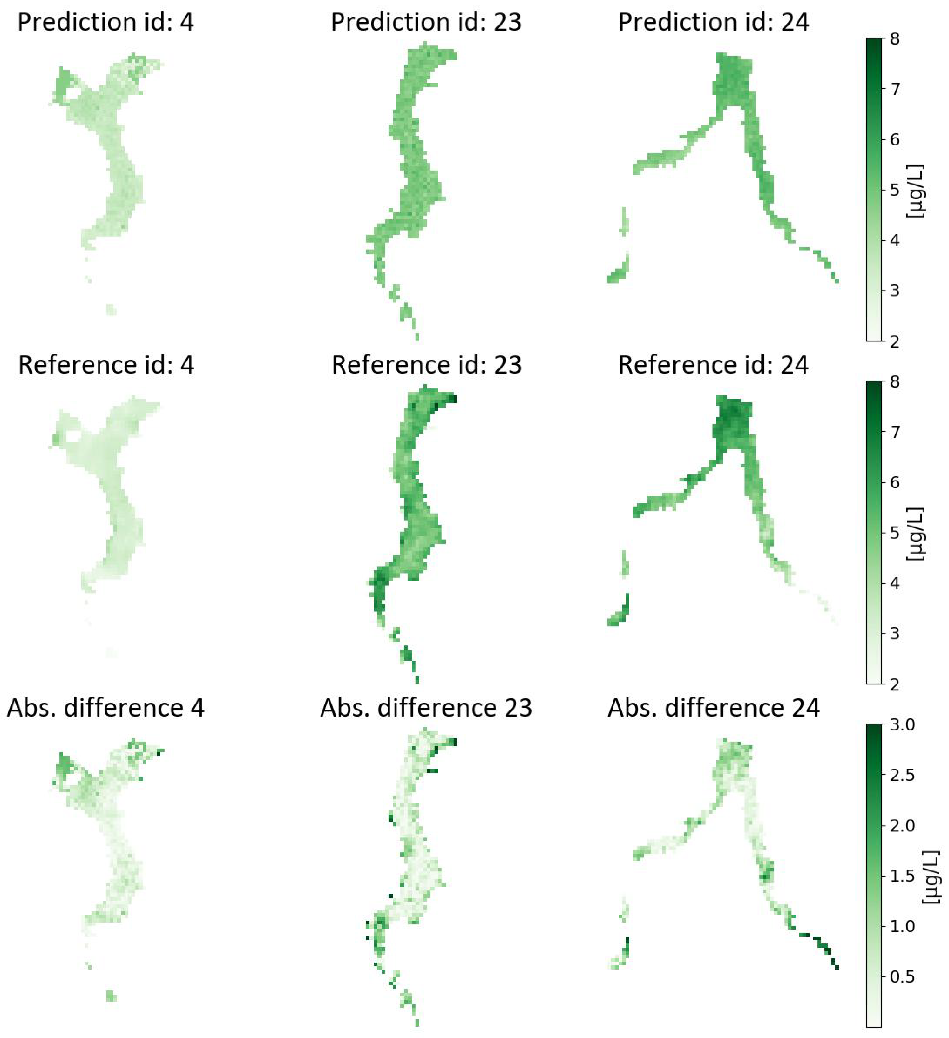
Figure 5 presents the visual results for Experiment SVR-4 with its model setting applied to the test acquisitions (ID 4, 23 and 24; see Table 1) and Figure 6 shows the distribution of the errors for each of the acquisitions in the test set.

Until this moment, the output spatial resolution of 300 m was overlooked, and only the resulting performance was analyzed. However, recognizing that output with a finer spatial resolution of 30 m could yield more valuable results, efforts were directed towards determining the optimal approach to achieve predictions at this higher resolution.

For this purpose, two alternative approaches were identified. The first, which has already been investigated, consisted of using 30-m data for model training, validation, and evaluation (testing). The second approach involved the use of the best-performing configurations of each considered model, which were trained with 300 m data (a summary of the results is included in Table 9), and to perform an inference on 30-m data for their evaluation. Figure 7 provides a schematic of these two alternative approaches.

After evaluating both approaches with the best-performing configurations of the four model typologies, the RF Regressor (Experiment RF-12) both trained and evaluated with 30-m data, emerged as the best alternative for achieving a prediction with 30 m of spatial resolution. The summary of these results is reported in

Table 10. Comparison of metrics for the best-performing configuration for each model using 30 m spatial resolution data, applied for each of the acquisitions in the test set. Training set (Train res.) and evaluation set (Eval. res) spatial resolutions are reported in dedicated columns. Overall MAE and RMSE represent the average scores for the metrics obtained from applying the experiments to each of the acquisitions in the test set. Values are reported in [µg/L].

Exp. ID	Model	Train. Res. [m]	Eval. Res. [m]	MAE Overall	RMSE Overall	MAE-4	RMSE-4	MAE-23	RMSE-23	MAE-24	RMSE-24
RF-10	RF	300	30	1.076	1.241	0.988	1.071	0.836	1.068	1.405	1.585
RF-12	RF	30	30	0.986	1.181	0.815	0.921	0.707	0.987	1.435	1.635
SVR-4	SVR	300	30	1.107	1.266	1.578	1.620	0.778	1.017	0.964	1.161
SVR-10	SVR	30	30	1.260	1.555	1.052	1.571	1.043	1.235	1.686	1.859
LSTM-13	LSTM	300	30	1.234	1.369	0.826	0.905	1.413	1.556	1.462	1.648
LSTM-14	LSTM	30	30	1.278	1.455	1.004	1.112	1.004	1.214	1.826	2.039
GRU-8	GRU	300	30	1.248	1.393	0.643	0.746	1.294	1.448	1.808	1.986
GRU-17	GRU	30	30	1.203	1.382	0.598	0.727	1.518	1.732	1.493	1.686

.

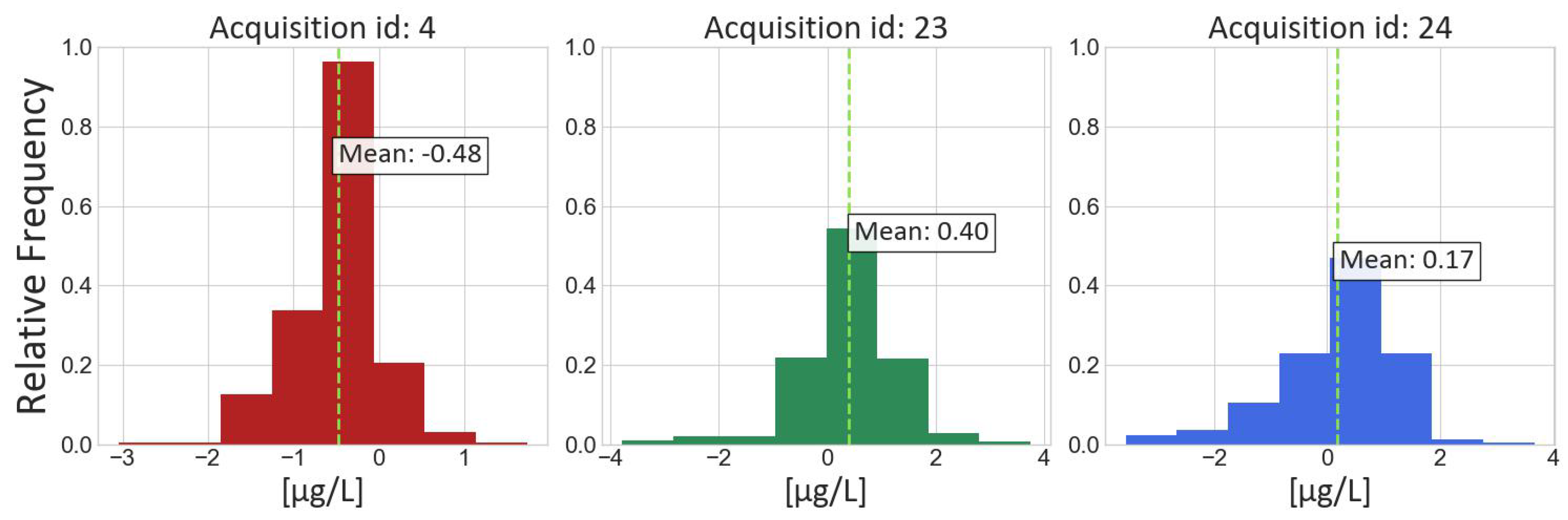
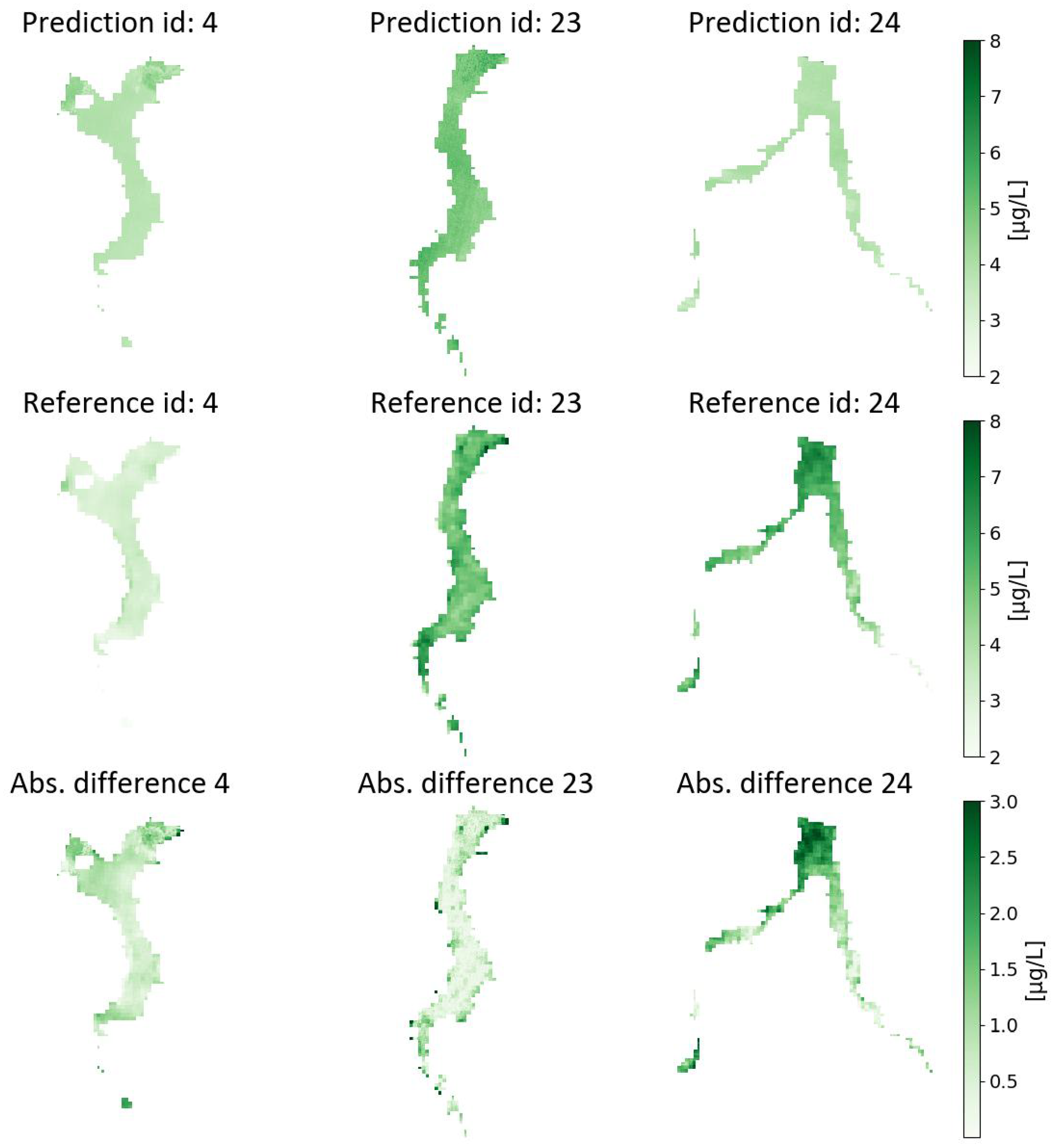
Figure 8 presents the visual results of Experiment RF-12, trained and evaluated at 30-m spatial resolution data and applied to each of the acquisitions in the test set. The associated errors’ distributions are shown in Figure 9.

A final observation drawn from the presented results is the tendency of the considered machine learning models to underestimate Chl-a values in high local concentration spots. Further considerations on the above are reported in the following section.

4. Conclusions and Outlook

This study addressed the implementation aspects related to the generation of Chl-a concentration maps utilizing PRISMA hyperspectral imagery, with low-resolution training data derived from Sentinel-3 imagery. The complete workflow for preparing input data for a range of machine and deep learning models was outlined. Performances of the models under various hyperparameter configurations were compared to offer empirical insights into the best-performing solutions for estimating multi-resolution Chl-a concentrations in lakes using hyperspectral imagery and pre-existing Chl-a concentration maps at lower spatial but higher temporal resolution.

By conducting several modelling experiments, the optimal configurations for each of the four analyzed models were determined. Specifically, the most favourable performances were attained when employing 300 m spatial resolution inputs for all experiments. The best results were achieved with the SVR model. Supplementary experiments were conducted to evaluate model performances in enhancing the spatial resolution of Chl-a concentration predictions from the original 300 m reference data (i.e., Sentinel-3 derived Chl-a concentration maps) to 30 m resolution such as the one of PRISMA hyperspectral imagery. The RF Regressor proved to deliver the best performance for this last objective.

While the obtained performances are relevant for all model typologies, it is worth noting that these results could be potentially improved with the availability of additional PRISMA acquisitions. As discernible from the presented results, the selected machine learning models demonstrated a tendency to underestimate regions characterized by high Chl-a concentrations. The inclusion of supplementary PRISMA acquisitions linked to high Chl-a concentration spots in the input dataset (which were limited in the dataset used for this study) is expected to mitigate this discrepancy and represents a critical improvement for future developments of this work.

Given the limitations to the accessibility of ground truth data for training and evaluating machine and deep learning models, the approach outlined in this study is promising for preliminary large-scale estimates of Chl-a concentrations in freshwater bodies. This is because it suggests strategies for the use of low-resolution and widely accessible training and testing datasets by leading to a final product with a significantly higher spatial resolution than the reference data while maintaining an acceptable margin of error. This enhancement is achieved by leveraging both spectral and spatial characteristics of the emerging hyperspectral satellite imagery. It is worth remarking that operations such as resampling low-resolution reference data for model evaluation on 30 m resolution outputs were tested for purely experimental purposes. The use of high-resolution reference data is envisaged to improve both the quality and reliability of the proposed procedure, especially of local gradients of Chl-a concentrations in each single water body.

The outcomes of the suggested method have the potential to function as supportive resources for the monitoring and administration of the lakes under investigation. The use of global coverage and freely available data, coupled with open modelling tools, additionally strengthens this groundwork for enhancements and replications in different geographic regions.

References

1. Vollenweider, R.; Kerekes, J. Eutrophication of Waters: Monitoring, Assessment and Control; OECD: Wiley, Hoboken, NJ, USA, 1982. [Google Scholar]
2. Bhagowati, B.; Ahamad, K.U. A review on lake eutrophication dynamics and recent developments in lake modeling. Ecohydrol. Hydrobiol. 2019, 19, 155–166. [Google Scholar] [CrossRef]
3. Grizzetti, B.; Liquete, C.; Pistocchi, A.; Vigiak, O.; Zulian, G.; Bouraoui, F.; De Roo, A.; Cardoso, A. Relationship between ecological condition and ecosystem services in European rivers, lakes and coastal waters. Sci. Total Environ. 2019, 671, 452–465. [Google Scholar] [CrossRef] [PubMed]
4. United Nations. Transforming our world: The 2030 Agenda for Sustainable Development. 2015. Available online: https://sdgs.un.org/2030agenda (accessed on 7 November 2023).
5. Schindler, D.W.; Carpenter, S.R.; Chapra, S.C.; Hecky, R.E.; Orihel, D.M. Reducing phosphorus to curb lake eutrophication is a success. Environ. Sci. Technol. 2016, 50, 8923–8929. [Google Scholar] [CrossRef] [PubMed]
6. Wetzel, R.G.; Likens, G. Limnological Analyses; Springer Science & Business Media: Berlin/Heidelberg, Germany, 2000. [Google Scholar]
7. Kahlert, M.; McKie, B.G. Comparing new and conventional methods to estimate benthic algal biomass and composition in freshwaters. Environ. Sci. Process. Impacts 2014, 16, 2627–2634. [Google Scholar] [CrossRef]
8. Guyot, G.; Baret, F.; Jacquemoud, S. Imaging Spectroscopy for Vegetation Studies; Kluwer Academic Publishers: Norwell, MA, USA, 1992; Volume 2. [Google Scholar]
9. Gohin, F.; Van der Zande, D.; Tilstone, G.; Eleveld, M.A.; Lefebvre, A.; Andrieux-Loyer, F.; Blauw, A.N.; Bryère, P.; Devreker, D.; Garnesson, P.; et al. Twenty years of satellite and in situ observations of surface chlorophyll-a from the northern Bay of Biscay to the eastern English Channel. Is the water quality improving? Remote Sens. Environ. 2019, 233, 111343. [Google Scholar] [CrossRef]
10. Maier, P.M.; Keller, S. Estimating chlorophyll a concentrations of several inland waters with hyperspectral data and machine learning models. arXiv 2019, arXiv:1904.02052. [Google Scholar] [CrossRef]
11. Lioumbas, J.; Christodoulou, A.; Katsiapi, M.; Xanthopoulou, N.; Stournara, P.; Spahos, T.; Seretoudi, G.; Mentes, A.; Theodoridou, N. Satellite remote sensing to improve source water quality monitoring: A water utility’s perspective. Remote Sens. Appl. Soc. Environ. 2023, 32, 101042. [Google Scholar] [CrossRef]
12. Giardino, C.; Brando, V.; Gege, P.; Pinnel, N.; Hochberg, E.; Knaeps, E.; Reusen, I.; Doerffer, R.; Bresciani, M.; Braga, F.; et al. Imaging spectrometry of inland and coastal waters: State of the art, achievements and perspectives. Surv. Geophys. 2019, 40, 401–429. [Google Scholar] [CrossRef]
13. Hafeez, S.; Wong, M.S.; Abbas, S.; Asim, M. Evaluating landsat-8 and sentinel-2 data consistency for high spatiotemporal inland and coastal water quality monitoring. Remote Sens. 2022, 14, 3155. [Google Scholar] [CrossRef]
14. Hestir, E.L.; Brando, V.E.; Bresciani, M.; Giardino, C.; Matta, E.; Villa, P.; Dekker, A.G. Measuring freshwater aquatic ecosystems: The need for a hyperspectral global mapping satellite mission. Remote Sens. Environ. 2015, 167, 181–195. [Google Scholar] [CrossRef]
15. Ma, T.; Zhang, D.; Li, X.; Huang, Y.; Zhang, L.; Zhu, Z.; Sun, X.; Lan, Z.; Guo, W. Hyperspectral remote sensing technology for water quality monitoring: Knowledge graph analysis and Frontier trend. Front. Environ. Sci. 2023, 11. [Google Scholar] [CrossRef]
16. Dierssen, H.M.; Ackleson, S.G.; Joyce, K.E.; Hestir, E.L.; Castagna, A.; Lavender, S.; McManus, M.A. Living up to the hype of hyperspectral aquatic remote sensing: Science, resources and outlook. Front. Environ. Sci. 2021, 9. [Google Scholar] [CrossRef]
17. Folkman, M.A.; Pearlman, J.; Liao, L.B.; Jarecke, P.J. EO-1/Hyperion hyperspectral imager design, development, characterization, and calibration. Hyperspectral Remote Sens. Land Atmos. 2001, 4151, 40–51. [Google Scholar]
18. Alonso, K.; Bachmann, M.; Burch, K.; Carmona, E.; Cerra, D.; De los Reyes, R.; Dietrich, D.; Heiden, U.; Hölderlin, A.; Ickes, J.; et al. Data products, quality and validation of the DLR earth sensing imaging spectrometer (DESIS). Sensors 2019, 19, 4471. [Google Scholar] [CrossRef]
19. Guanter, L.; Kaufmann, H.; Segl, K.; Foerster, S.; Rogass, C.; Chabrillat, S.; Kuester, T.; Hollstein, A.; Rossner, G.; Chlebek, C.; et al. The EnMAP spaceborne imaging spectroscopy mission for earth observation. Remote Sens. 2015, 7, 8830–8857. [Google Scholar] [CrossRef]
20. Liu, Y.N.; Sun, D.X.; Hu, X.N.; Ye, X.; Li, Y.D.; Liu, S.F.; Cao, K.Q.; Chai, M.Y.; Zhang, J.; Zhang, Y.; et al. The advanced hyperspectral imager: Aboard China’s gaoFen-5 satellite. IEEE Geosci. Remote Sens. Mag. 2019, 7, 23–32. [Google Scholar] [CrossRef]
21. Cogliati, S.; Sarti, F.; Chiarantini, L.; Cosi, M.; Lorusso, R.; Lopinto, E.; Miglietta, F.; Genesio, L.; Guanter, L.; Damm, A.; et al. The PRISMA imaging spectroscopy mission: Overview and first performance analysis. Remote Sens. Environ. 2021, 262, 112499. [Google Scholar] [CrossRef]
22. Esposito, M.; Marchi, A.Z. In-orbit demonstration of the first hyperspectral imager for nanosatellites. In Proceedings of the International Conference on Space Optics—ICSO, Chania, Greece, 9–12 October 2018; Volume 11180, pp. 760–770. [Google Scholar] [CrossRef]
23. Qian, S.E. Hyperspectral satellites, evolution, and development history. IEEE J. Sel. Top. Appl. Earth Obs. Remote Sens. 2021, 14, 7032–7056. [Google Scholar] [CrossRef]
24. Audebert, N.; Le Saux, B.; Lefèvre, S. Deep learning for classification of hyperspectral data: A comparative review. IEEE Geosci. Remote Sens. Mag. 2019, 7, 159–173. [Google Scholar] [CrossRef]
25. Shi, K.; Zhang, Y.; Qin, B.; Zhou, B. Remote sensing of cyanobacterial blooms in inland waters: Present knowledge and future challenges. Sci. Bull. 2019, 64, 1540–1556. [Google Scholar] [CrossRef] [PubMed]
26. Gholizadeh, M.H.; Melesse, A.M.; Reddi, L. A comprehensive review on water quality parameters estimation using remote sensing techniques. Sensors 2016, 16, 1298. [Google Scholar] [CrossRef] [PubMed]
27. Ali, K.A.; Ortiz, J.D. Multivariate approach for chlorophyll-a and suspended matter retrievals in Case II type waters using hyperspectral data. Hydrol. Sci. J. 2016, 61, 200–213. [Google Scholar] [CrossRef]
28. Sun, D.; Li, Y.; Wang, Q. A unified model for remotely estimating chlorophyll a in Lake Taihu, China, based on SVM and in situ hyperspectral data. IEEE Trans. Geosci. Remote Sens. 2009, 47, 2957–2965. [Google Scholar]
29. Keller, S.; Maier, P.M.; Riese, F.M.; Norra, S.; Holbach, A.; Börsig, N.; Wilhelms, A.; Moldaenke, C.; Zaake, A.; Hinz, S. Hyperspectral data and machine learning for estimating CDOM, chlorophyll a, diatoms, green algae and turbidity. Int. J. Environ. Res. Public Health 2018, 15, 1881. [Google Scholar] [CrossRef]
30. Maier, P.M.; Keller, S. Application of different simulated spectral data and machine learning to estimate the chlorophyll a concentration of several inland waters. In Proceedings of the 2019 10th Workshop on Hyperspectral Imaging and Signal Processing: Evolution in Remote Sensing (WHISPERS), Amsterdam, The Netherlands, 24–26 September 2019; IEEE: Piscataway, NJ, USA, 2019; pp. 1–5. [Google Scholar]
31. Ali, K.A.; Moses, W.J. Application of a PLS-augmented ANN model for retrieving chlorophyll-a from hyperspectral data in case 2 waters of the western basin of Lake Erie. Remote Sens. 2022, 14, 3729. [Google Scholar] [CrossRef]
32. Maier, P.M.; Keller, S.; Hinz, S. Deep learning with WASI simulation data for estimating chlorophyll a concentration of inland water bodies. Remote Sens. 2021, 13, 718. [Google Scholar] [CrossRef]
33. Saberioon, M.; Khosravi, V.; Brom, J.; Gholizadeh, A.; Segl, K. Examining the sensitivity of simulated EnMAP data for estimating chlorophyll-a and total suspended solids in inland waters. Ecol. Inform. 2023, 75, 102058. [Google Scholar] [CrossRef]
34. Segl, K.; Guanter, L.; Rogass, C.; Kuester, T.; Roessner, S.; Kaufmann, H.; Sang, B.; Mogulsky, V.; Hofer, S. EeteS—The EnMAP End-to-End Simulation Tool. IEEE J. Sel. Top. Appl. Earth Obs. Remote Sens. 2012, 5, 522–530. [Google Scholar] [CrossRef]
35. Pahlevan, N.; Smith, B.; Binding, C.; Gurlin, D.; Li, L.; Bresciani, M.; Giardino, C. Hyperspectral retrievals of phytoplankton absorption and chlorophyll-a in inland and nearshore coastal waters. Remote Sens. Environ. 2021, 253, 112200. [Google Scholar] [CrossRef]
36. Lima, T.M.A.d.; Giardino, C.; Bresciani, M.; Barbosa, C.C.F.; Fabbretto, A.; Pellegrino, A.; Begliomini, F.N. Assessment of Estimated Phycocyanin and Chlorophyll-a Concentration from PRISMA and OLCI in Brazilian Inland Waters: A Comparison between Semi-Analytical and Machine Learning Algorithms. Remote Sens. 2023, 15, 1299. [Google Scholar] [CrossRef]
37. Mosher, T.; Mitchell, M. Hyperspectral imager for the coastal ocean (HICO). In Proceedings of the 2004 IEEE Aerospace Conference Proceedings (IEEE Cat. No. 04TH8720), Biloxi, MS, USA, 26–29 October 2009; IEEE: Piscataway, NJ, USA, 2004; Volume 1. [Google Scholar]
38. Yuan, Q.; Shen, H.; Li, T.; Li, Z.; Li, S.; Jiang, Y.; Xu, H.; Tan, W.; Yang, Q.; Wang, J.; et al. Deep learning in environmental remote sensing: Achievements and challenges. Remote Sens. Environ. 2020, 241, 111716. [Google Scholar] [CrossRef]
39. Brovelli, M.; Cannata, M.; Rogora, M. Simile, a geospatial enabler of the monitoring of sustainable development goal 6 (ensure availability and sustainability of water for all). Int. Arch. Photogramm. Remote Sens. Spat. Inf. Sci. 2019, 42, 3–10. [Google Scholar] [CrossRef]
40. Luciani, G.; Bresciani, M.; Biraghi, C.A.; Ghirardi, N.; Carrion, D.; Rogora, M.; Brovelli, M.A. Satellite Monitoring system of Subalpine lakes with open source software: The case of SIMILE Project. Balt. J. Mod. Comput. 2021, 9, 135–144. [Google Scholar] [CrossRef]
41. Amieva, J.; Austoni, A.; Bresciani, M.; Brovelli, M. Analysis of the Remotely Sensed Water Quality Parameters of the Insubric Lakes: Methods and Results of the Interreg Simile Project. Int. Arch. Photogramm. Remote Sens. Spat. Inf. Sci. 2023, 48, 9–16. [Google Scholar] [CrossRef]
42. Toro Herrera, J.; Carrion, D.; Bresciani, M.; Bratić, G. Semi-automated production and filtering of satellite derived water quality parameters. Int. Arch. Photogramm. Remote Sens. Spat. Inf. Sci. 2022, 43, 1019–1026. [Google Scholar] [CrossRef]
43. Hochreiter, S.; Schmidhuber, J. Long short-term memory. Neural Comput. 1997, 9, 1735–1780. [Google Scholar] [CrossRef]
44. Gers, F.A.; Schmidhuber, J.; Cummins, F. Learning to forget: Continual prediction with LSTM. Neural Comput. 2000, 12, 2451–2471. [Google Scholar] [CrossRef] [PubMed]
45. Cho, K.; van Merriënboer, B.; Gulcehre, C.; Bahdanau, D.; Bougares, F.; Schwenk, H.; Bengio, Y. Learning phrase representations using RNN encoder-decoder for statistical machine translation. In Proceedings of the 2014 Conference on Empirical Methods in Natural Language Processing (EMNLP), Doha, Qatar, 25–29 October 2014; Association for Computational Linguistics: Stroudsburg, PA, USA, 2014; pp. 1724–1734. [Google Scholar]
46. Agency, I.S. PRISMA Products Specification Document—Issue 2.3; Italian Space Agency: Rome, Italy, 2020. [Google Scholar]
47. Plyer, A.; Colin-Koeniguer, E.; Weissgerber, F. A new coregistration algorithm for recent applications on urban SAR images. IEEE Geosci. Remote Sens. Lett. 2015, 12, 2198–2202. [Google Scholar] [CrossRef]
48. Gilerson, A.; Gitelson, A.; Zhou, J.G.D.; Moses, W.; Ioannou, I.; Ahmed, S. Algorithms for remote estimation of chlorophyll-a in coastal and inland waters using red and near infrared bands. Opt. Express 2010, 8, 24109–24125. [Google Scholar] [CrossRef]
49. ESA. Radiometric Resolution—21 bands in VIS/SWIR. 2023. Available online: https://sentinels.copernicus.eu/web/sentinel/user-guides/sentinel-3-olci/resolutions/radiometric (accessed on 7 November 2023).
50. Bresciani, M.; Adamo, M.; De Carolis, G.; Matta, E.; Pasquariello, G.; Vaičiūtė, D.; Giardino, C. Monitoring blooms and surface accumulation of cyanobacteria in the Curonian Lagoon by combining MERIS and ASAR data. Remote Sens. Environ. 2014, 146, 124–135. [Google Scholar] [CrossRef]
51. Mobley, C.D. Light and Water: Radiative Transfer in Natural Waters; JSTOR: New York, NY, USA, 1994. [Google Scholar]
52. Agenzia Spaziale Italiana (ASI). PRISMA Product Specification. 2020. Available online: https://prisma.asi.it/missionselect/docs/PRISMA%20Product%20Specifications_Is2_3.pdf (accessed on 22 May 2023).
53. Sobel, I. An isotropic 3 × 3 image gradient operator. In Proceedings of the 5th Annual Symposium on Theory of Computing, Austin, TX, USA, 30 April–2 May 1973; ACM: New York, NY, USA, 1973; pp. 271–272. [Google Scholar]
54. Gonzalez, R.C.; Woods, R.E. Digital Image Processing, 4th ed.; Pearson: London, UK, 2018. [Google Scholar]
55. Breiman, L. Random forests. Mach. Learn. 2001, 45, 5–32. [Google Scholar] [CrossRef]
56. Drucker, H.; Wu, D.; Vapnik, V.N. Support vector regression machines. Adv. Neural Inf. Process. Syst. 1997, 9, 155–161. [Google Scholar]
57. Pedregosa, F.; Varoquaux, G.; Gramfort, A.; Michel, V.; Thirion, B.; Grisel, O.; Blondel, M.; Prettenhofer, P.; Weiss, R.; Dubourg, V.; et al. Scikit-learn: Machine Learning in Python. J. Mach. Learn. Res. 2011, 12, 2825–2830. [Google Scholar]
58. Scikit-Learn. Random Forest Regressor. 2023. Available online: https://scikit-learn.org/stable/modules/generated/sklearn.ensemble.RandomForestRegressor.html (accessed on 22 May 2023).
59. Scikit-Learn. Support Vector Machines. 2023. Available online: https://scikit-learn.org/stable/modules/svm.html (accessed on 22 May 2023).
60. Oguiza, I. tsai—A State-of-the-Art Deep Learning Library for Time Series and Sequential Data. 2022. Available online: https://github.com/timeseriesAI/tsai (accessed on 22 May 2023).
61. Srivastava, N.; Hinton, G.; Krizhevsky, A.; Sutskever, I.; Salakhutdinov, R. Dropout: A simple way to prevent neural networks from overfitting. J. Mach. Learn. Res. 2014, 15, 1929–1958. [Google Scholar]
Figure 1. Summary of available data (pixels with information of Chl-a maps and PRISMA acquisitions) within the study’s AOI. In the reference map is highlighted the approximate location of the AOI within Europe (red dot).
Remotesensing 15 05385 g001
Figure 2. Schematic of pre-processing operations on the input data.
Remotesensing 15 05385 g002
Figure 3. Schematic of the anomalous pixels removal procedure.
Remotesensing 15 05385 g003
Figure 4. QQ-plot of training and test sets. Blue dots represent quantiles of pixel values distribution from reference Chl-a maps in the training set (X-axis) and test set (Y-axis).
Remotesensing 15 05385 g004
Figure 5. Predictions and reference Chl-a map and their absolute difference (Abs. difference) computed from Experiment SVR-4 applied to each of the acquisitions in the test set.
Remotesensing 15 05385 g005
Figure 6. Distribution of the errors of Experiment SVR-4 applied to each of the acquisitions in the test set.
Remotesensing 15 05385 g006
Figure 7. Schematic of the inference procedures on 30 m spatial resolution output.
Remotesensing 15 05385 g007
Figure 8. Predictions and reference Chl-a map and their absolute difference (Abs. difference) computed from Experiment RF-12 trained and evaluated at 30-m spatial resolution data and applied to each of the acquisitions in the test set.
Remotesensing 15 05385 g008
Figure 9. Distribution of the errors of Experiment RF-12 trained and evaluated at 30-m spatial resolution data and applied to each of the acquisitions in the test set.
Remotesensing 15 05385 g009