Surface Motion and Topographic Effects on Ice Thickness Inversion for High Mountain Asia Glaciers: A Comparison Study from Three Numerical Models

Abstract

Several studies have evaluated the accuracy of ice thickness model inversions, but the effects of surface velocity and topographic factors have not been fully studied. Because of the important potential of models for estimating regional and global ice thickness, the influence of the characteristics of the glaciers themselves on the models is unknown. Therefore, we estimated the thickness of 10 glaciers in HMA based on remote sensing data using the GlabTop2, GV22, and VOLTA models, and we analyzed the factors affecting accuracy. The first two models are representative of the widely used shallow ice approximation and laminar flow theory, and the latter is a new model based on shallow ice approximation. The results show that the RMSEs for GlabTop2, VOLTA, and GV22 are 36.6 m, 56.8 m, and 63.2 m, respectively. The accuracy of the three models differed obviously under the influence of different slopes, aspects, and surface velocities. In contrast to glaciers with higher surface velocities, GV22 is more suitable for glaciers with smaller surface velocities, and the accuracy of the model is significantly reduced when surface velocities are greater than 50 m/yr. Aspect has an effect on the accuracy of the GV22 ice thickness inversion but not on the other models. Ice thicknesses estimated using the three models is more reliable at surface slopes of 16–24°. These three models do not apply to gentle glaciers such as icecaps. Our study provides an important reference for choosing a suitable model to invert the glacier thickness in HMA.

1. Introduction

Glacier thickness distribution is one of the basic preconditions for solving numerous glaciological and hydrological problems [1,2]. Continued global warming will lead to increased glacier melting, which will alter the mass balance, movement characteristics, and local geomorphology of glaciers [3,4,5]. This increases the risk of glacier disasters such as ice avalanches, glacier surging, and glacial lake outburst floods, posing severe threats to life safety and infrastructure downstream [6,7,8]. At the same time, the rapid response of the cryosphere to rising temperatures will also change the spatial and temporal distribution of the global climate and precipitation [3]. Therefore, using remote sensing data to estimate glacier thickness over large areas is of great significance for studying the future evolution of available water resources, glacier disaster prevention, sea level changes, and glacier dynamics [1,5,7,9]. Currently, glacier thickness measurement techniques include radio echo, drilling, seismic, gravity, etc. However, in situ observations of glacier thickness are sparse due to the high cost of observation, the harsh environment, and the inaccessibility for humans and equipment [10,11]. The latest release of the Glacier Thickness Database (GlaThiDa v3) included only 4000 glaciers worldwide [12]. For ~200,000 glaciers globally, this still seems to be an insufficient observation, so numerical models are widely used for global ice thickness inversion [13,14].

At present, scholars have developed more than 17 models that use remote sensing data or empirical parameters to invert ice thickness and volume [13,15]. Among them, GlabTop2, based on shallow ice approximation (SIA) theory, and the ice flow model, based on laminar flow theory, are widely used [16,17]. In addition, based on the SIA theory, centerline ice thickness can also be interpolated to obtain the glacier thickness distribution using models such as VOLTA [18]. Existing studies have used these models to estimate global or regional glacier thickness and evaluate model performance [15,17]. However, these studies are limited to accuracy assessment, and research on how glacier characteristics (such as glacier surface slope, slope aspect, ice velocity, etc.) affect the accuracy of ice thickness model inversion is still insufficient.

High Mountain Asia (HMA) is the largest glaciated area outside the polar regions, and glacial meltwater sustains a population of 250 million people in Asia [9]. Many previous studies have been conducted on HMA glaciers using ice thickness models (e.g., based on glacier outlines, DEM, and glacier surface velocity) [15,16,19]. Various approaches to estimating glacier volumes have been proposed, such as volume–area (V–A) relations, slope-dependent ice thickness estimations, and, more recently, a variety of spatially distributed ice thickness models [20,21,22,23,24]. V-A, GlabTop2, laminar flow, H-F, and multi-model synthesis have been used to estimate HMA glacier volumes of 12,484 km³, 5282 km³, 9400 km³, 4693 km³, and 7020 km³, respectively [9,15,17,25,26]. In summary, there are significant differences in the available results, and therefore the accuracy of the ice thickness model for HMA needs to be evaluated.

The models currently available all invert glacier thickness using several remote sensing variables (e.g., glacier outlines, slope, surface velocity, etc.). The accuracy of these variables as input data to the model directly affects the ice thickness results. In addition, differences in solar radiation received from different aspects can affect the accuracy of ice thickness estimates. To assess the effect of uncertainty in these variables on glacier volume, some authors have carried out a series of sensitivity tests and assessed the uncertainty [1,16]. Uncertainties in ice thickness and total glacier volume based on laminar flow equation simulations are usually quantified using error propagation. The sensitivity of ice thickness to basal velocity values was estimated [21]. The sensitivity of glacier volume and ice thickness to other variables was estimated by varying the shallow ice approximation theory’s shape factor and shear stress [16,27]. A method for determining valley shape factors based on glacier width was proposed [18,28,29]. In addition, input data can affect the accuracy of ice thickness estimates. Previous studies have analyzed the effect of different DEM and glacier outline data on ice thickness estimation [10,30]. However, these studies ignore the effect of glacier characteristics (e.g., slope, aspect, velocity, etc.) on model estimates of ice thickness, which may lead to overestimation or underestimation of ice thickness in the model. We summarize the applicability of the models by analyzing their performance under different glacial features.

In this study, we used three models to invert glacier thickness at different locations in HMA. The purpose was to assess the models’ performance for the estimation of glacier ice thickness in HMA. Firstly, we calculated the ice thickness distribution of ten glaciers in the HMA area using the GlabTop2, GV22, and VOLTA models based on remote sensing data (DEM, glacier outline, and surface velocity). Then, we utilized the GPR measurement data to assess the three models’ uncertainty. We quoted six different evaluation indexes to assess the reliability of the three models. The applicability of these models was discussed by considering the effects of glacier surface slope, aspect, and surface velocity on ice thickness estimation. Finally, a series of sensitivity tests were performed to analyze the effects of variables on the modeled ice thickness.

2. Study Area and Datasets

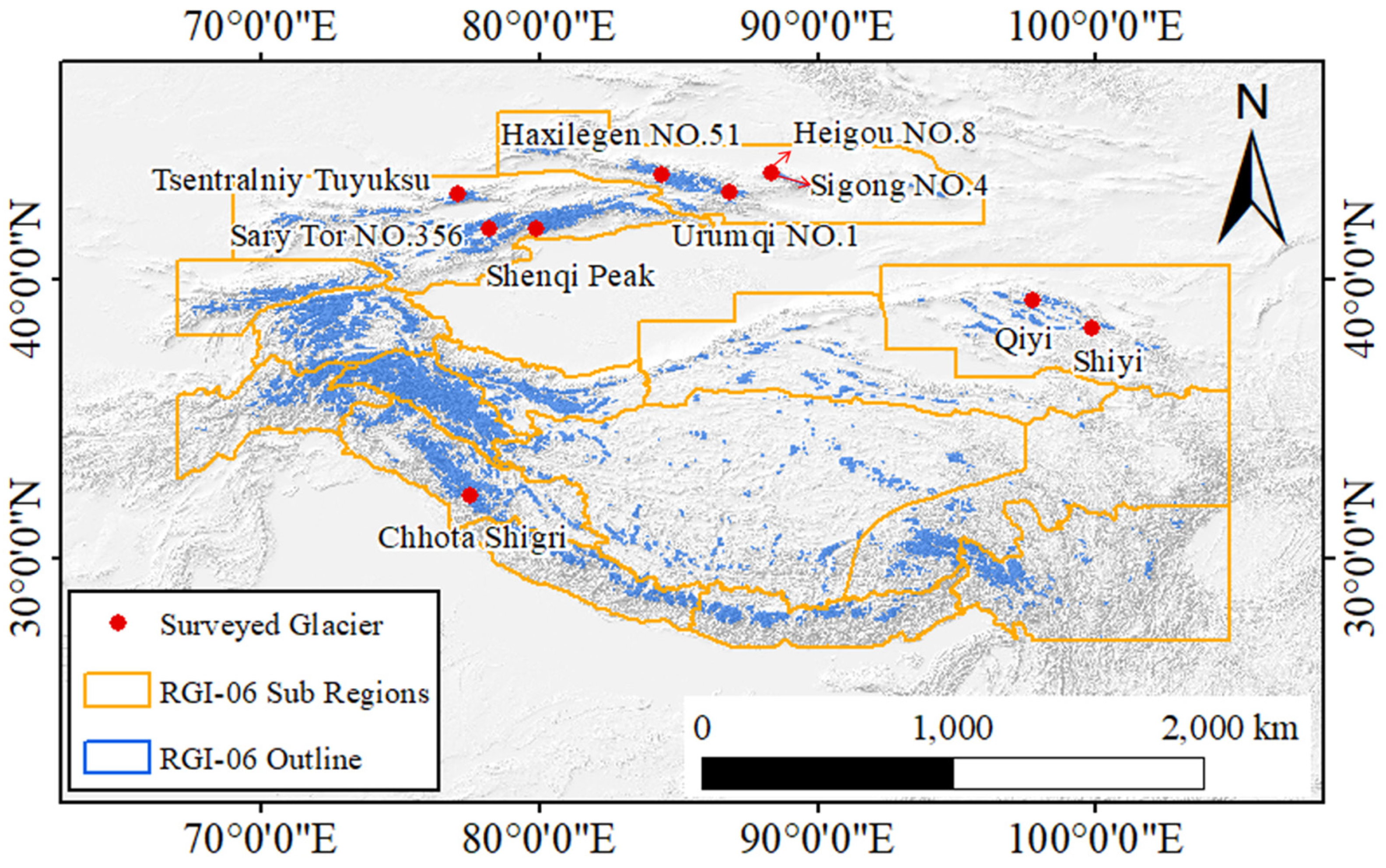
2.1. Study Area

HMA, which consists of the Tibetan Plateau and its surrounding mountain ranges (including the Himalayas, Karakoram Range, Tien Shan Range, and Pamir Range), has the highest concentration of glaciers outside the poles, and is therefore known as the “Third Pole” [31]. These glaciers are the headwater of many rivers, such as the Yangtze River, the Brahmaputra, and the Lancang River. Therefore, HMA is commonly known as the Asian Water Tower. The latest version of the Randolph Glacier Inventory (RGI-60) includes 95536 glaciers over HMA, covering an area of 97,605 ± 7935 km² [32]. Among the 10 glaciers studied, Chhota Shigri is located in the Himalaya Mountains, Qiyi and Shiyi glaciers are located in the Qilian Mountains, and the others are located in the Tian Shan region (Figure 1). The Qiyi and Shiyi Glacier in the Qilian Mountains are mainly influenced by the East Asian monsoon, while the other glaciers are influenced by the westerlies. The influences of atmospheric circulation patterns and topography can lead to differences in precipitation and glacial dynamics, as well as different glacial mass balances [3,33].

2.2. Datasets

In order to assess the accuracy of the modeled ice thickness estimates, we compiled a considerable number of ice thickness measurements acquired using GPR surveys from GlaThiDa [12] and ITMIX2 [34], spanning 1980 to 2014. GlaThiDa is an open database on glacier thickness from the Global Terrestrial Network for Glaciers (GTN-G) published by the WGMS (https://wgms.ch/, accessed on 7 July 2022). GlaThiDa is a collection of worldwide ice thickness measurements. There are nine HMA glaciers represented in GlaThiDa v3, together accounting for 14749 points with ice thickness measured using GPR. We also obtained GPR measurements of Chhota Shigri’s thickness [34,35].

To reduce the influence of different topographies and glacier outlines at different timestamps on the ice thickness estimate result, two DEMs were used: the Shuttle Radar Topography Mission (SRTM) DEM and the Copernicus DEM GLOB-30 (hereafter COPDEM30) [36,37,38]. The SRTM was launched on 11 February 2000, acquired images from both X- and C-band Synthetic Aperture Radar, and captured the surface of the globe from 60°N latitude to 56°S latitude. The current SRTM, v3 (http://earthexplorer.usgs.gov, accessed on 24 September 2021), with a 30 m grid cell size, was released in 2014. The absolute vertical and relative accuracies of SRTM3 are 16 m and 10 m, respectively. Copernicus DEM (COPDEM30) (https://registry.opendata.aws/copernicus-dem, accessed on 10 April 2022) is global and was reprocessed from WorldDEM^TM products by resampling, filling holes, replacing abnormal values, etc. The source data for WorldDEM^TM were acquired during the 2011–2015 TanDEM-X mission [10,39]. There are currently three Copernicus DEM products, GLOB-30, GLOB-90, and EEA-10. The absolute vertical and relative accuracies of the Copernicus DEM are 4 m and 2 m, respectively. In this study, we used COPDEM30 to estimate the slope and aspect around 2013. To minimize the impact of different timestamps on the data, we used two DEMs (

Table 1. GPR measurement information and DEMs used.

ID	Glacier	DEM	Source	Time	Area_(km2)
1	Urumqi No.1	COPDEM30	GlaThiDa	2014	1.581
2	Sigonghe No.4	COPDEM30	GlaThiDa	2009	2.643
3	Sary-Tor	COPDEM30	GlaThiDa	2013	2.925
4	Shiyi	COPDEM30	GlaThiDa	2010	0.495
5	Haxilegen No.51	COPDEM30	GlaThiDa	2010	1.099
6	Heigou No.8	COPDEM30	GlaThiDa	2009	6.078
7	Shenqi Peak	COPDEM30	GlaThiDa	2008	6.595
8	Qiyi	SRTM-C	GlaThiDa	1980	2.531
9	Tsentralniy Tuyuksu	COPDEM30	GlaThiDa	2013	2.838
10	Chhota Shigri	COPDEM30	[34,35]	2009	16.764

).

Solar radiation directly affects the mass balance on the glacier surface, runoff, etc., and thus the estimation of glacier thickness. For this purpose, we also used land surface temperature (LST) data [40,41]. It uses the thermal infrared remote sensing data merging method to reconstruct the all-weather LST of China and its neighboring areas, using Terra/Aqua MODIS LST products and CLDAS and other data as inputs. The dataset has a spatial resolution of 1 km and can be downloaded from the National Tibetan Plateau Data Center (https://data.tpdc.ac.cn, accessed on 4 June 2023).

The glacier surface velocity data used in this study are from Millan et al. (2022) [17]. This article describes the calculation of global glacier surface velocities with cross-correlation methods using 2017–2018 Landsat8, Sentinel-1, and Sentinel-2 data [17,42]. Then, the thickness of 98% of the world’s glaciers was calculated using laminar flow theory (https://doi.org/10.6096/1007, accessed on 27 February 2022). The spatial resolution of the glacier surface velocity and ice thickness data is 50 m.

3. Methods

3.1. GlabTop2 Ice Thickness Model Description

Linsbauer et al. [43] established the GlabTop model to reconstruct the subglacial topography based on geographic information system (GIS) technology, which relies on the mechanics of SIA. First, GlabTop is used to estimate the ice thickness along the centerline. Then, glacier ice thickness distribution is derived by interpolating between the centerline and the glacier margins. The thickness of the glacier margin is 0. However, GlabTop requires a manual process of drawing branch lines. Frey et al. [16] developed a new version of GlabTop (GlabTop2) that simplifies the process of estimating ice thickness. GlabTop2 is a grid-based and slope-dependent model used to estimate glacier ice thickness. Ice thickness guesses at randomly selected cells are based on the assumption of perfect plasticity [16].

$$h_f=\frac{\tau }{f\rho gsin\left(\mathsf{\alpha }\right)}$$

(1)

where $h_f$ (m) is the ice thickness, $\rho$ is the density of ice ($900\mathrm{k}\mathrm{g}·{\mathrm{m}}^{-3}$), $g$ is the acceleration of gravity (${9.81\mathrm{m}·\mathrm{s}}^{-2}$), and $\mathsf{\alpha }$ (°) is the surface slope. $f$ is a dimensionless shape factor that accounts for drag by valley walls, which depends on the ratio of the half-width to the midpoint depths on the centerline [29]. τ (kPa) is the average basal shear stress, the value of which is estimated from an empirical relation proposed by Haeberli and Hoelzle [44]. GlabTop2 requires only the glacier mask, DEM, and surface slope as input data. Glacier thickness is obtained by interpolating a randomly selected set of estimated ice thickness cells.

3.2. VOLTA Ice-Thickness Inversion Model

James and Carrivick [18] developed a VOLTA model that generates a centerline network automatically based on the GIS hydrological tool. VOLTA is a Python script based on Arcpy, which is based on the assumption of perfect plasticity. The model uses the DEM and glacier outline as input data to estimate centerline ice thickness. Then, the glacier ice thickness distribution is derived by interpolating between the centerline and the glacier margins [18,45]. VOLTA’s definition of glacier thickness is along the plumb line. Therefore, the detailed formula of VOLTA is as follows:

$$h_f=\frac{\tau }{f\rho gtan\left(\mathsf{\alpha }\right)}$$

(2)

The basal shear stress is estimated from the area–slope relationship proposed by Driedger and Kennard [46]. Firstly, VOLTA was used to determine the geometric centerline of the glacier, and the surface slope and elevation range were combined to calculate the thickness of the ice on the centerline. Then, the thickness of the glacier area was obtained by interpolation with the Australian National University DEM (ANUDEM). Unlike the glacier surface thickness along the vertical direction to the ice bed calculated by GlabTop2, VOLTA obtains the ice thickness along the gravity direction to the ice bed.

3.3. Ice Velocity-Based Model Description

Surface velocities were calculated using the subpixel correlation of the images [47,48]. Ice thickness is estimated using the equation of laminar flow [21]:

$$h=\sqrt[4]{\frac{v_s(1-\beta )(n+1)}{2A{\left({\rho }_{m}gsin\mathsf{\alpha }\right)}^n}}$$

(3)

where $h$ (m) is the ice thickness; $v_s$ is the surface velocity; $\beta$ is the ratio between glacier basal and surface velocity; n is the exponent in Glen’s [49] law, usually taken as n = 3; A is the creep parameter; ${\rho }_m$ is the ice density, ${917\mathrm{k}\mathrm{g}·\mathrm{m}}^{-3}$; $g$ is the gravitational acceleration, usually taken as ${9.81\mathrm{m}\mathrm{s}}^{-2}$; and, α is the glacier surface slope [17,21,42].

In this study, glacier surface velocity and ice thickness estimated using the laminar flow model are taken from Millan et al. (hereafter GV22) [17]. Remote sensing imagery was processed using subpixel correlation to obtain glacier surface flow velocities for the period 2017–2018 [17]. Ice thickness was calculated for 98% of global glaciers using velocities based on a laminar flow model. The ice thickness product has a resolution of 50 m and an accuracy of 10m a⁻¹. The HMA glacier volume of $9.6\pm 3.7\times {10}^3{\mathrm{k}\mathrm{m}}^3$ represents 7% of the global alpine glacier volume and an equivalent sea level of 24.3 ± 10.5 mm.

3.4. Accuracy Assessment

We used six different accuracy metrics to comprehensively assess the accuracy of the three models in modeling ice thickness. The six different accuracy indexes are mean absolute error (MAE), root mean square error (RMSE), standard deviation (STD), relative error (RE), Nash–Sutcliffe efficiency (NSE), and correlation coefficient (Corr) [27,50,51,52]. The detailed formula explanation is as follows:

$$\mathrm{M}\mathrm{A}\mathrm{E}=\frac{{\displaystyle {\sum }_{i=1}^n}\left|H_{GPR}-H_{mod}\right|}{n}$$

(4)

$$\mathrm{R}\mathrm{M}\mathrm{S}\mathrm{E}=\sqrt{\frac{{\displaystyle {\sum }_{i=1}^n}{(H_{GPR}-H_{mod})}^2}{n}}$$

(5)

$$\mathrm{S}\mathrm{T}\mathrm{D}=\sqrt{\frac{{\displaystyle {\sum }_{i=1}^n}{(H_{GPR}-H_{mod}-\frac{1}{n}{\displaystyle {\sum }_{i=1}^n}(H_{GPR}-H_{mod}))}^2}{n-1}}$$

(6)

$$\mathrm{N}\mathrm{S}\mathrm{E}=1-\frac{{\displaystyle {\sum }_{i=1}^n}{(H_{GPR}-H_{mod})}^2}{{\displaystyle {\sum }_{i=1}^n}{(H_{GPR}-\frac{1}{n}{\displaystyle {\sum }_{i=1}^n}{H}_{GPR})}^2}$$

(7)

$$\mathrm{R}\mathrm{E}=\frac{H_{GPR}-H_{mod}}{H_{GPR}}$$

(8)

$$\mathrm{C}\mathrm{o}\mathrm{r}\mathrm{r}=\frac{{\displaystyle {\sum }_{i=1}^n}\left(\right(H_{GPR}-\frac{1}{n}{\displaystyle {\sum }_{i=1}^n}{H}_{GPR}\left)\right(H_{mod}-\frac{1}{n}{\displaystyle {\sum }_{i=1}^n}{H}_{mod}\left)\right)}{\sqrt{{\displaystyle {\sum }_{i=1}^n}{(H_{GPR}-\frac{1}{n}{\displaystyle {\sum }_{i=1}^n}{H}_{GPR})}^2}\sqrt{{\displaystyle {\sum }_{i=1}^n}{(H_{mod}-\frac{1}{n}{\displaystyle {\sum }_{i=1}^n}{H}_{mod})}^2}}$$

(9)

where $H_{GPR}$ is the ice thickness measured using GPR and $H_{mod}$ is the ice thickness measured using the model.

The mean absolute error (MAE) prevents errors from canceling each other out. RMSE is a measure of the normalized distance between the measured and simulated ice thickness that allows for an assessment of the bias between the model and the GPR. The standard deviation (STD) can describe the dispersion of the estimated ice thickness. The Nash efficiency (NSE) coefficient is used to evaluate the quality of the model results. The correlation coefficient can reflect the closeness of the estimated ice thickness and GPR.

4. Results and Analysis

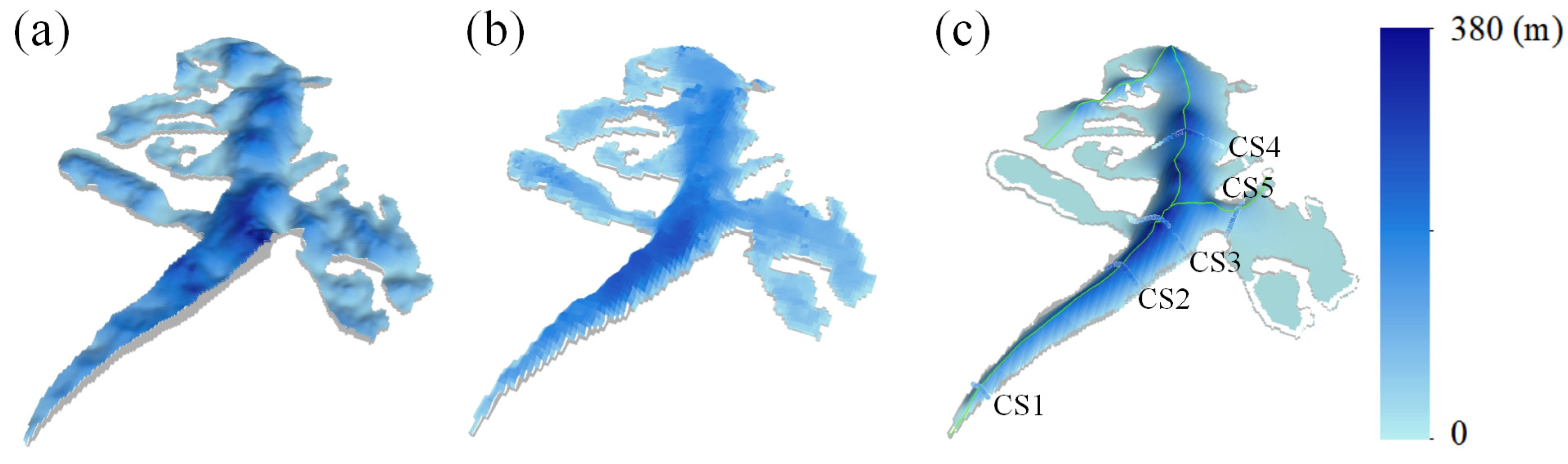
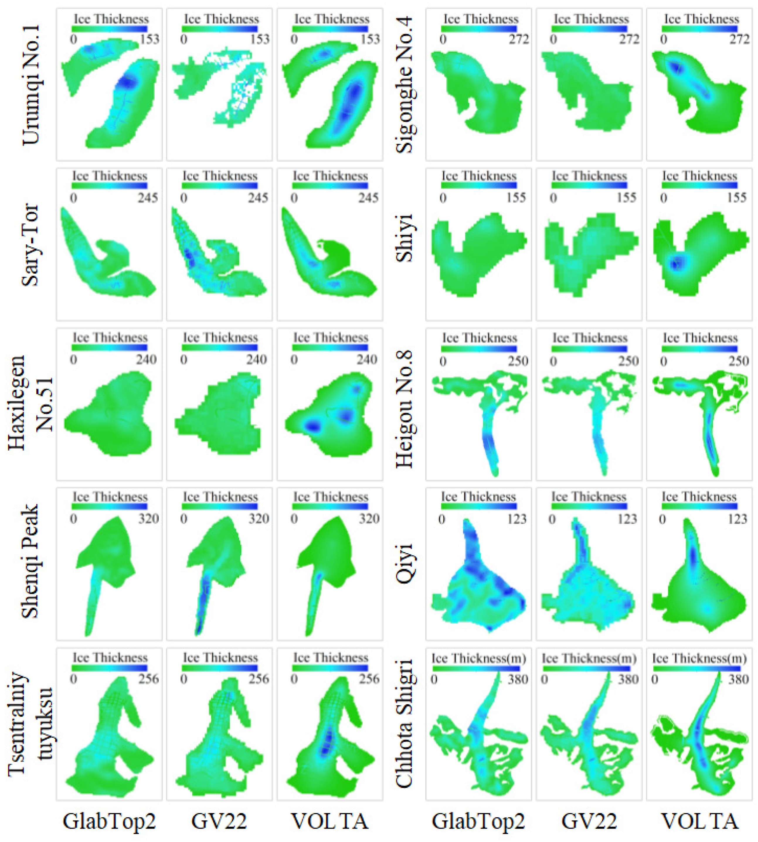
4.1. Spatial Distribution of Simulated Ice Thickness

The GlabTop2 model parameters for estimating the thickness of alpine glaciers are discussed using the Chhota Shigri glacier as an example. We calibrated the shape factor, which usually ranges from 0.6 to 0.9 [28]. The RMSE value is minimized when the shape factor is 0.87. The random grid-cell density of the GlabTop2 was set to 30%. Repeating the ice thickness calculation three times is important in the GlabTop2 model. The thickness of the glacier margin is 0 [16]. Based on the above parameters, GlabTop2 was used to estimate the glacier thickness distribution (Figure 2a). The Chhota Shigri glacier has a maximum thickness of 295.41 m and is located near CS3 (cross-section 3). The average ice thickness of the glacier is 96.35 m, with an area of 13.48 km² and a volume of 1.30 km³. The thickness distribution of the Chhota Shigri glacier was estimated based on glacier velocity (Figure 2b). Here, we used the ice thickness estimated by Millan et al. (2022). The maximum and average ice thicknesses are 269 m and 98.4 m, respectively. Unlike the GlabTop2 model, the maximum ice thickness simulated using GV22 is located at CS2. The glacier volume is 1.30 km³, which is consistent with GlabTop2 (

Table 2. Glacier thickness and ice volume estimated using different models (GlabTop2 (GT2)).

Glacier	Area (km2)	Average Ice Thickness at Measurement Sites (m)				Volume (km3)			Maximum Ice Thickness (m)			RE (%)
		GPR	GT2	GV22	VOLTA	GT2	GV22	VOLTA	GT2	GV22	VOLTA	GT2	GV22	VOLTA
Urumqi No.1	1.58	69.95	64.45	57.47	66.82	0.077	0.073	0.074	153.37	98.41	149.05	−7.86	−17.84	−4.47
Sigonghe No.4	2.64	68.87	88.61	59.22	121.26	0.122	0.103	0.143	130.41	81.38	272.23	28.66	−14.01	76.07
Sary-Tor	2.93	75.47	77.87	106.30	75.65	0.177	0.234	0.131	132.97	245.49	189.82	3.18	40.85	0.24
Shiyi	0.50	39.27	39.96	34.42	42.50	0.012	0.015	0.013	56.02	62.79	155.01	1.76	−12.35	8.23
Haxilegen No.51	1.10	43.89	46.61	63.10	96.62	0.037	0.045	0.072	77.20	100.80	240.10	6.20	43.77	120.14
Heigou No.8	6.07	114.83	142.21	129.78	150.40	0.431	0.358	0.269	214.60	166.68	246.27	23.84	13.02	30.98
Shenqi Peak	6.59	38.65	106.54	200.79	72.81	0.338	0.536	0.206	172.17	314.60	246.81	175.65	419.51	88.38
Qiyi	2.53	76.82	76.70	61.21	41.61	0.158	0.133	0.063	123.13	109.96	118.94	−0.16	−20.32	−45.83
Tsentralniy Tuyuksu	2.84	50.92	72.80	86.79	80.43	0.151	0.178	0.137	137.43	170.11	256.55	42.97	70.44	57.95
Chhota Shigri	13.48	172.88	176.01	161.29	135.32	1.299	1.300	0.872	295.41	268.76	379.46	1.81	−6.70	−21.73

).

In addition, we estimated the ice thickness distribution of the Chhota Shigri glacier using the VOLTA model. Firstly, VOLTA generates a primary centerline and two branch centerlines and calculates the centerline ice thickness. Then, the ANUDEM interpolation method was used to obtain the glacier thickness distribution. The glacier thickness distribution was obtained by interpolating the ice thickness at the centerlines and glacier margin using ANUDEM (Figure 2c). As can be seen from the figure, the ice thickness shows a decreasing trend from the centerline to the edge, with the maximum ice thickness located near the centerline at about 379 m. The average ice thickness and volume of the glacier are 75.53 m and 0.87 km³, respectively (Table 2). The estimated ice thickness at CS3 is greater than the GPR measurements, while it is smaller at CS1 and CS5.

As can be seen in Figure 2b, the VOLTA model does not even generate centerlines in some tributaries. This leads to an underestimation of tributary ice thickness. The maximum ice thickness estimated using the VOLTA model lies strictly on the glacier centerline. Furthermore, due to the complex geometry of the glacier outline, the generated glacier centerline may cross the glacier outline, requiring manual correction of the centerline. Therefore, the VOLTA model needs to increase the centerline density to describe the spatial distribution of ice thickness in detail. GlabTop2 and GV22 invert ice thickness based on randomly selected cells and glacier velocity, respectively. These two models describe the details of ice thickness variations within the outline better than VOLTA.

Figure 3 shows the ice thickness results estimated using the GlabTop2, GV22, and VOLTA models at different sites. It is clear from the ice thickness results that there are significant differences in the distribution of glacier thicknesses estimated using the different methods. The thicknesses of glaciers Urumqi No.1, Sigonghe No.4, Shiyi, Haxilegen No.51, and Tsentralniy-Tuyuksu simulated using VOLTA are larger than those of the other two models and the GPR measurements. At the edges of glaciers Heigou No.8, Qiyi, and Tsentralniy-Tuyuksu, VOLTA estimates of ice thickness are smaller than the other two methods and close to zero. The basal shear stress of the GlabTop2 model was obtained from empirical relations and does not present spatial variations in shear stress. GlabTop2 estimates of glacier thickness for glaciers Urum No.1 and Sary-Tor are significantly lower than the GPR field data. Glacier ice thickness simulated using ice flow velocity is prone to missing cells and is affected by the remote sensing image quality. Urumqi glacier NO.1 can be taken as an example. In addition, there is a clear anomaly in the simulated thickness of the Shenqi Peak glacier.

Mean glacier thickness, glacier volume, and maximum ice thickness are statistically based on the model-estimated distribution of ice thickness (Table 2). The VOLTA model provides higher estimates of maximum ice thickness for six glaciers (Sigonghe No.4, Shiyi, Haxilegen No.51, Heigou No.8, Tsentralniy-Tuyuksu, and Chhota Shigri) than the other methods. This suggests that the VOLTA model is prone to extreme values in estimating ice thickness and is concentrated near the centerline. Five glaciers’ (Sary-Tor, Shiyi, Qiyi, Tsentralniy-Tuyuksu, and Chhota Shigri) volumes estimated using GV22 are higher than those from the other methods. GlabTop2 provides greater estimates of ice volume and maximum ice thickness for glaciers Urumqi No.1 and Qiyi than the other two models. This suggests that the GlabTop2 model performs more consistently than GV22 and VOLTA.

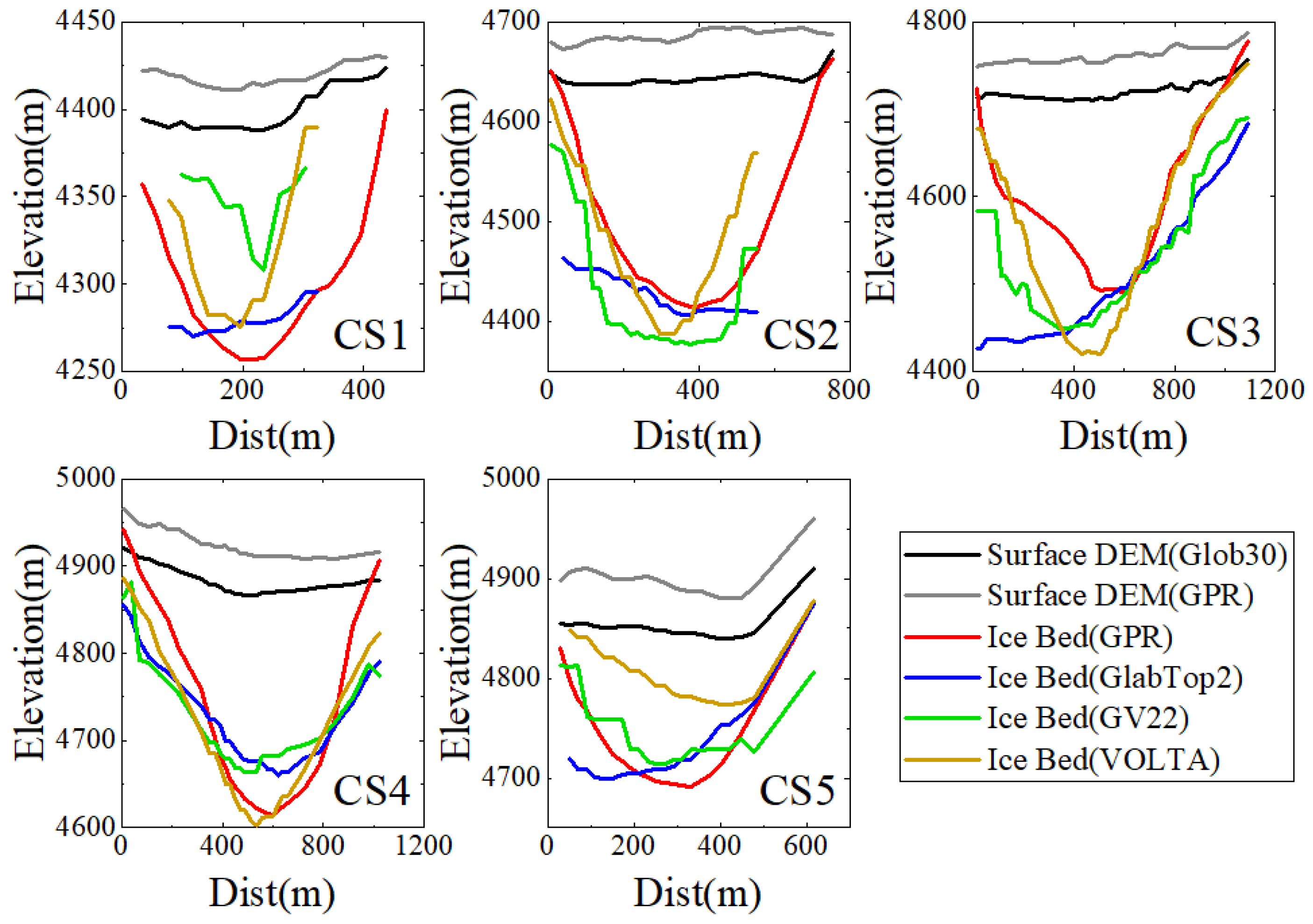
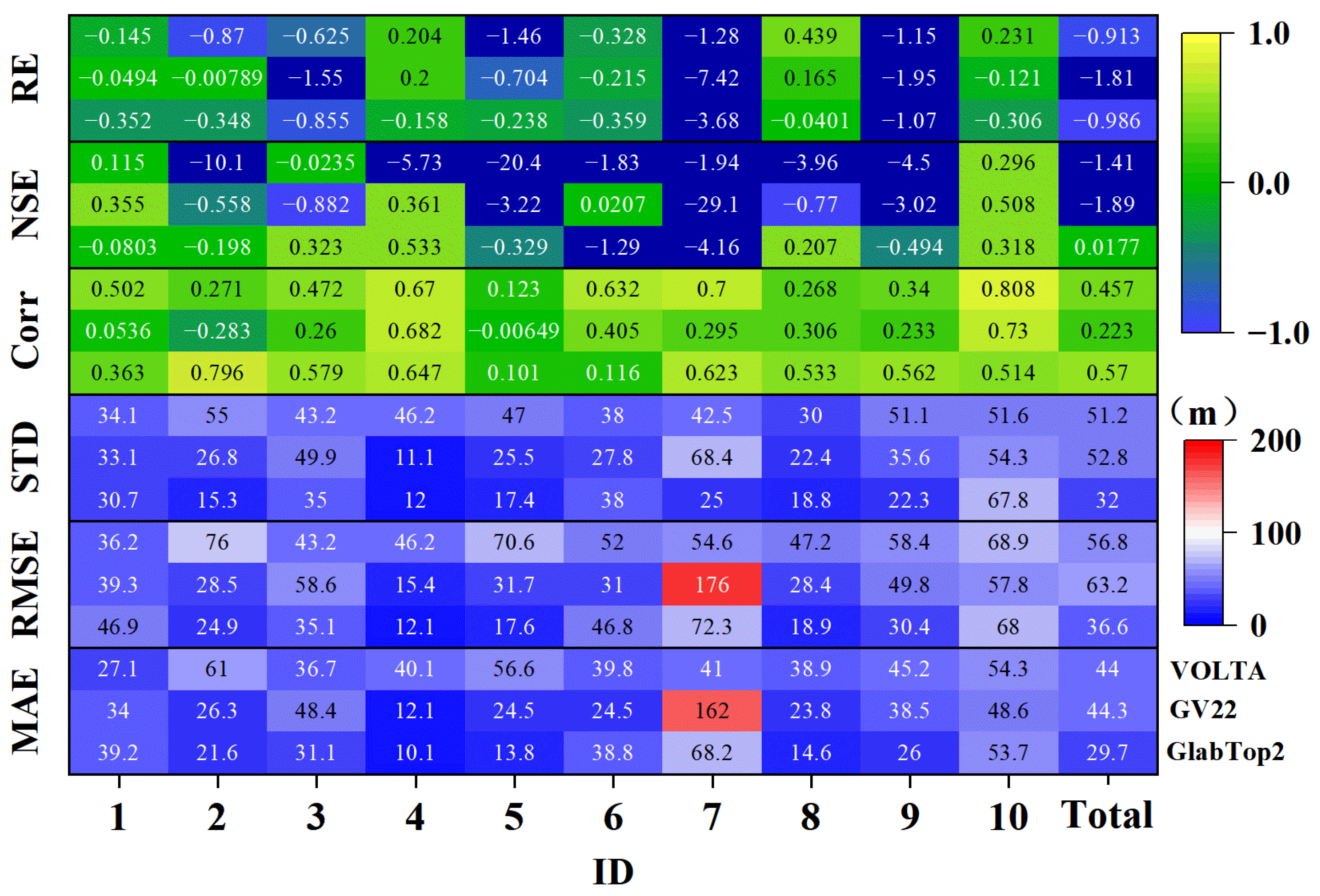
4.2. Accuracy of Simulated Ice Thickness

Using the Chhota Shigri glacier as an example, the accuracy of the different methods used to estimate ice thickness was analyzed. The modeled ice thickness at the location of the GPR measurement point was extracted (Figure 4) [28,35]. In cross-sections one and five, the accuracy of the GlabTop2 model is better than that of GV22 and VOLTA. In cross-sections two and three, GV22 has better accuracy than the other two models. In cross-section four, the VOLTA model is better. The RMSEs for simulated ice thickness were 67.82 m, 57.77 m, and 68.85 m for GlabTop2, GV22, and VOLTA, respectively. Overall, GV22 provides a more accurate estimate of Chhota Shigri glacier thickness than the GlabTop2 and VOLTA models. RMSEs were also calculated for the Chhota Shigri cross-section and overall ice thickness (

Table 3. RMSE in cross-section thicknesses of Chhota Shigri glacier.

Cross Section	RMSE
	GlabTop2	GV22	VOLTA
CS1	30.33	98.21	72.68
CS2	43.34	29.35	69.27
CS3	91.02	42.14	40.43
CS4	69.95	69.92	34.02
CS5	53.94	64.81	124.68
Total	67.82	57.77	68.85

).

Simulated thicknesses of the 10 glaciers were analyzed in comparison with GPR measurements (Figure 5). As can be seen from Figure 5, the modeled ice thickness results for glacier IDs 1, 3, 6, 8, and 10 are relatively consistent with the GPR measurements. Among them, the thickness of glacier 7 estimated using GV22 is significantly higher than that estimated using other models and GPR. The VOLTA model has higher estimated thicknesses for glacier IDs 2, 4, 7, and 9 than the GPR field data. This demonstrates the limitations of the GV22 and VOLTA models in estimating alpine glacier thickness, which is discussed in detail in Section 5.

The accuracy of the ice thickness simulated using the different methods was assessed using six metrics: MAE, RMSE, STD, Corr, NSE, and RE (Figure 6). Based on MAE and RMSE analyses, GlabTop2’s glacier thickness estimates for glacier IDs 2, 3, 4, 5, 8, and 9 are consistent with GPR measurements and outperform other models. GV22 estimated the thickness of ID 6 and 10 more accurately than GlabTop2 and VOLTA. The MAE and RMSE values for ID 7’s thickness estimated using GV22 are 162.02 m and 175.88 m, respectively, which are lower than the accuracy of the GlabTop2 and VOLTA models. VOLTA has higher accuracy in estimating the thickness of ID 1 and 7. The thickness of ID 4, estimated using GlabTop2, has the smallest MAE and RMSE values, which are 10.12m and 12.13 m, respectively. Overall, the GlabTop2 model has higher accuracy, with an RMSE of 36.55 m, better than VOLTA (56.84 m) and GV22 (63.19 m). According to the STD value analysis, the GlabTop2 model performed better on ID 1, 2, 3, 5, 7, 8, and 9; the GV22 model had higher accuracy on ID 4 and 6; and the VOLTA model performed better on ID 10. In the simulation results, GV22 estimated the minimum and maximum STD values for glacier thicknesses of ID 4 and 7, respectively. The STD value of ID 4 is 11.15 m, and that of ID 7 is 68.43 m. On the whole, the STD values for the GlabTop2, VOLTA, and GV22 are 31.99 m, 51.21 m, and 52.85 m respectively.

Based on the correlation coefficient analysis, the VOLTA model estimated higher correlation coefficients with GPR measurements for ID 1, 5, 6, 7, and 10 than the other models. Regarding ID 2, 3, 8, and 9, the GlabTop2 model had higher correlation coefficients than the other models, while for ID 4, the GV22 model had a higher correlation coefficient. Overall, the correlation coefficients for the GlabTop2, VOLTA, and GV22 models were 0.57, 0.46, and 0.22, respectively. According to the NSE coefficient analysis, GlabTop2 outperformed the other models in five glaciers, including ID 4, with an NSE value of 0.53, and GV22 outperformed the other models in four glaciers. VOLTA outperformed the other models only for ID 7, with an NSE value of −1.94, indicating that all three models had a large error in the estimated thickness of ID 7, which is consistent with the comparison results for ID 7 in Figure 5. The RE reflects the value by which the estimate deviates from the magnitude of the GPR measurement of ice thickness, with a plus or minus sign indicating an overestimate or underestimate. The simulated ice thicknesses of GlabTop2 all have negative RE values, indicating that the model results overestimate field data. The GlabTop2 model was superior to the other models in terms of RE values for the four glaciers. GV22 has smaller RE values on four glaciers, while simulated ice thicknesses on ID 4 and 8 are lower than those measured in situ.

To sum up, GlabTop2 is more stable and reliable in estimating glacier thickness and is superior to the GV22 and VOLTA models. The accuracy of the ice thickness of ID 7 estimated using GV22 is lower than that of other models and is analyzed in detail in Section 5.3. Except for the correlation coefficient, the accuracy of the VOLTA model results is lower than that of GlabTop2 for all other indexes. This shows that the interpolation of the VOLTA model along the centerline is prone to overestimation or underestimation.

5. Discussion

5.1. Comparison with Previous Research

There is a growing body of research on the thickness of alpine glaciers. To our knowledge, the thicknesses of the 10 glaciers of interest here have been studied using GPR measurements and inversion models [2,28,53]. To assess the reliability of the ice thickness estimated in this study, we compared it with the average ice thickness and volume estimated by Farinotti et al. [15].

Figure 7 shows the thickness of the 10 glaciers estimated using the different models. At ID 2, 4, 5, 6, 9, and 10, the maximum ice thickness estimated using VOLTA is significantly greater than the maximum ice thickness of the other simulations (Figure 7). The average ice thickness estimated using VOLTA is higher than that from the other models only at ID 2 and 5. This suggests that the maximum ice thickness estimated using the VOLTA model is overestimated, and the average ice thickness is underestimated, compared to the other models. At ID 3 and 7, the GV22 model estimated higher maximum and mean ice thicknesses than the other simulations. This suggests that the GV22 model has generally overestimated the ice thickness of some glaciers, which may be related to the characteristics of the glaciers themselves. This is discussed in Section 5.3 and Section 5.4. The GlabTop2 model simulates ice thicknesses closer to other models, with no obvious extremes. The main reasons for the differences from previous results are the differences in model parameters and the differences in input data accuracy, time period, and so on.

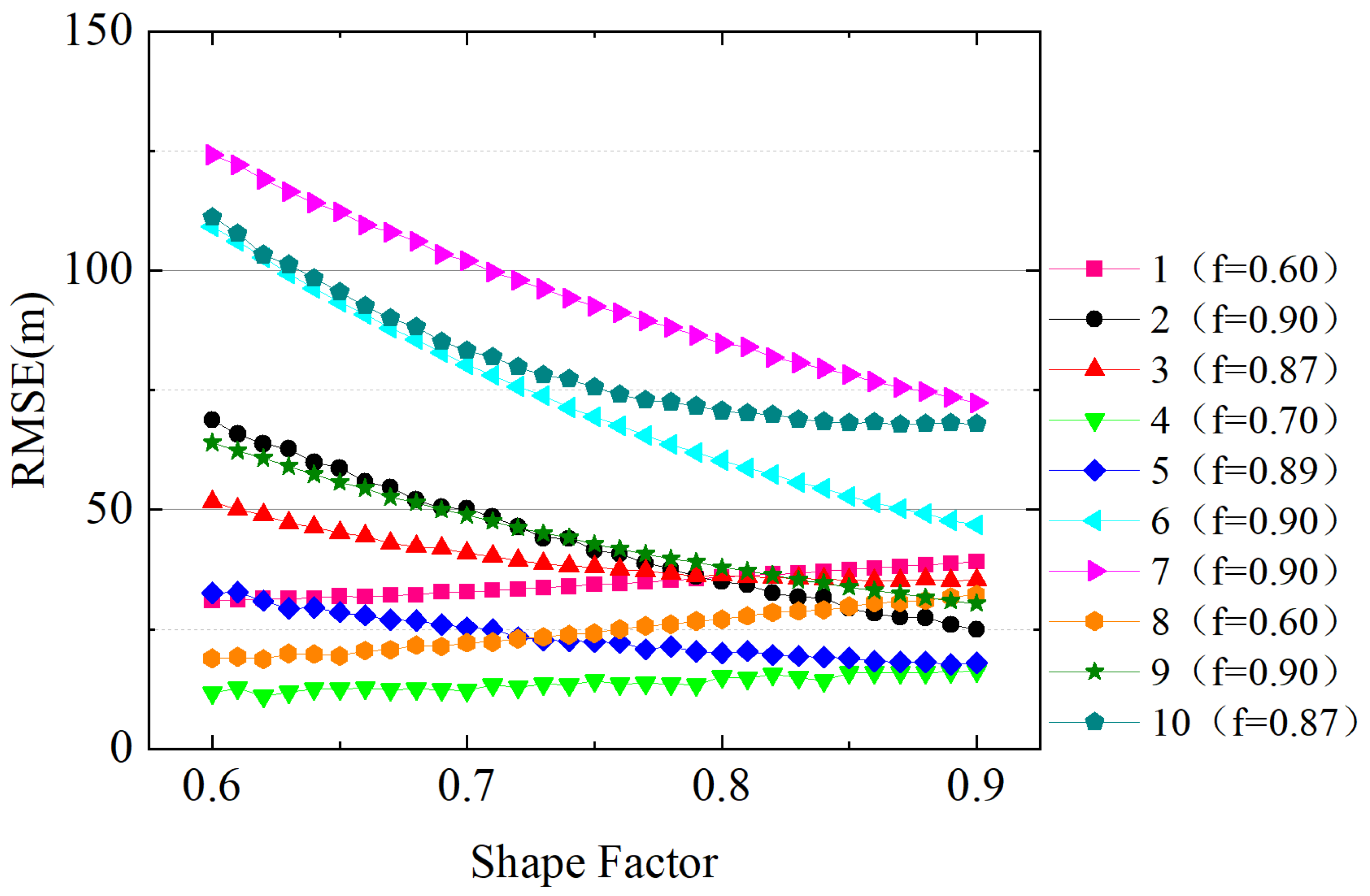
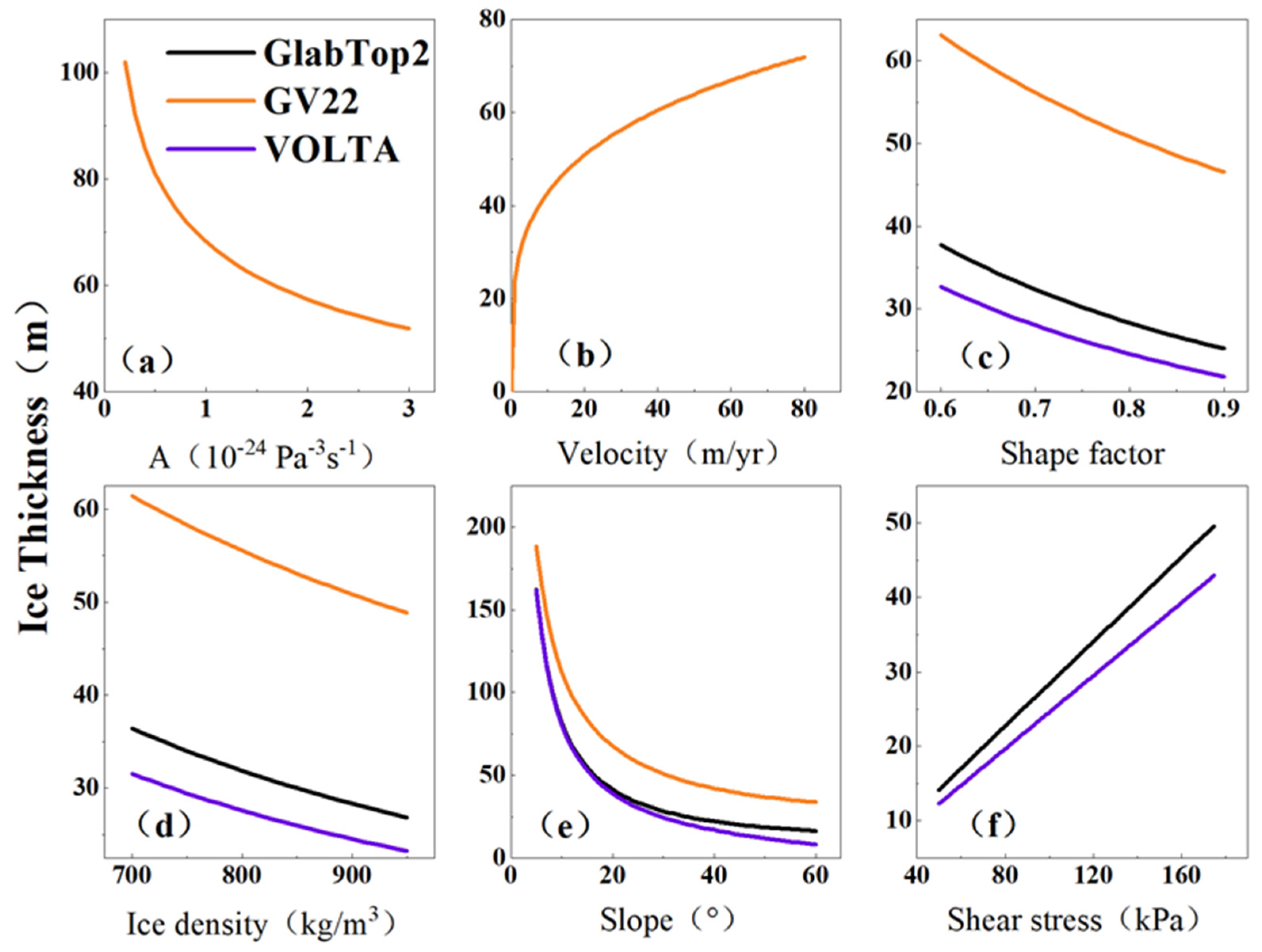
5.2. Sensitivity Analysis of Modeling

The parameters that affect the accuracy of the glacier thickness distribution simulated by the GlabTop2 mode are basal shear stress, valley shape factor, ice density, and surface slope [18,27,30,54]. In order to limit f to a reasonable range, we set f in the range of [0.6, 0.9] to select the optimal parameters based on previous studies [28]. This avoids overestimation or underestimation of ice thickness due to shape factor anomalies. The optimal valley shape factor is calibrated by calculating the RMSE values for different shape factor estimates of ice thickness. RMSE values of glacier thickness were calculated for glaciers with different shape factors (Figure 8). The optimal shape factor for each glacier is provided in the legend. As can be seen from the figure, each glacier has a different optimum shape factor. The trend in RMSE values varies with the shape factor. ID 2, 3, 5, 6, 7, 9, and 10 show a trend of decreasing RMSE with increasing shape factor, with an optimum shape factor range of 0.87 to 0.9. The RMSE values for ID 1, 4, and 8 show an increasing trend with increasing shape factor, with optimal shape factor spreading between 0.6 and 0.7. Therefore, the empirical value of 0.8 for the shape factor used in previous studies leads to errors in the ice thickness simulations [10,21].

Three models are used in this paper to simulate glacier thickness. Sensitivity analysis was carried out to analyze the effect of different variables on the ice thickness estimates. Variables that may affect ice thickness are discussed separately, such as creep parameter, valley shape factor, glacier surface velocity, ice density, basal shear stress, and glacier surface slope (Figure 9). The variation in estimated ice thickness for different creep parameters ($3.24\times {10}^{-24}{Pa}^{-3}{s}^{-1}$) is approximately ±2.4% when A is varied by 3.1% ($0.1\times {10}^{-24}{Pa}^{-3}{s}^{-1}$) (Figure 9a). There is a change in ice thickness of approximately 1.43% for every 1m a-1 change in glacier surface velocity (Figure 9b). When the shape factor was changed by 0.1, the GlabTop2, GV22, and VOLTA models estimated changes in ice thickness of ±1.3%, ±1.0%, and ±1.3%, respectively (Figure 9c). The different sensitivities of the three models to f are due to theoretical differences. For a $10\mathrm{k}\mathrm{g}·m^{-3}$ change in ice density, the ice thickness estimated using the three models varied by ±1.2%, ±0.9%, and ±1.2% respectively (Figure 9d). For each 1° change in glacier surface slope, the three models simulated changes in ice thickness of ±5.9%, ±4.6%, and ±7.1%, respectively (Figure 9e). For a 10 kPa variation in basal shear stress, the GlabTop2 and VOLTA models estimate a variation in ice thickness of ±10.8% (Figure 9f). In summary, the order of sensitivity of the GlabTop2 and VOLTA models to the input variables is basal shear stress, surface slope, shape factor, and ice density. The sensitivity of the GV22 model to the input variables, in order, is surface slope, creep parameter, surface velocity, shape factor, and ice density, which is consistent with previous results [54]. In addition, our results show that highly accurate input data are important to improve the accuracy of ice thickness estimates, such as DEM and glacier outlines.

5.3. Influence of Glacier Velocity on Ice Thickness Estimate

The accuracy of the ice thickness inversion model may also be influenced by glacier characteristics such as surface velocity and aspect [27,54]. We analyzed the possible influence of surface velocity on the bias in estimating glacier thickness (Figure 10). K1 and K2 represent the slopes of the trends in ice thickness deviation for surface velocities less than 50 m/year and greater than 50 m/year, respectively. As can be seen from the graph, when the glacier velocity exceeds 50 m/year, the deviation in ice thickness estimated using the GV22 model increases significantly (K1 = −0.47 to K2 = −3.73, Figure 10). According to Equation (3), GV22 takes glacier velocity as an input and the estimated ice thickness increases with increasing velocity. However, glacier velocity is affected by factors such as topography and temperature. This indicates that the GV22 model is too dependent on surface velocity in estimating glacier thickness and is not applicable to fast-flowing glaciers. The GlabTop2 and VOLTA models use basal shear stress as an input, and the deviation in estimated ice thickness is not affected by surface velocity. As a result, the bias in ice thickness estimated using GlabTop2 and VOLTA remains distributed around zero as the velocity increases.

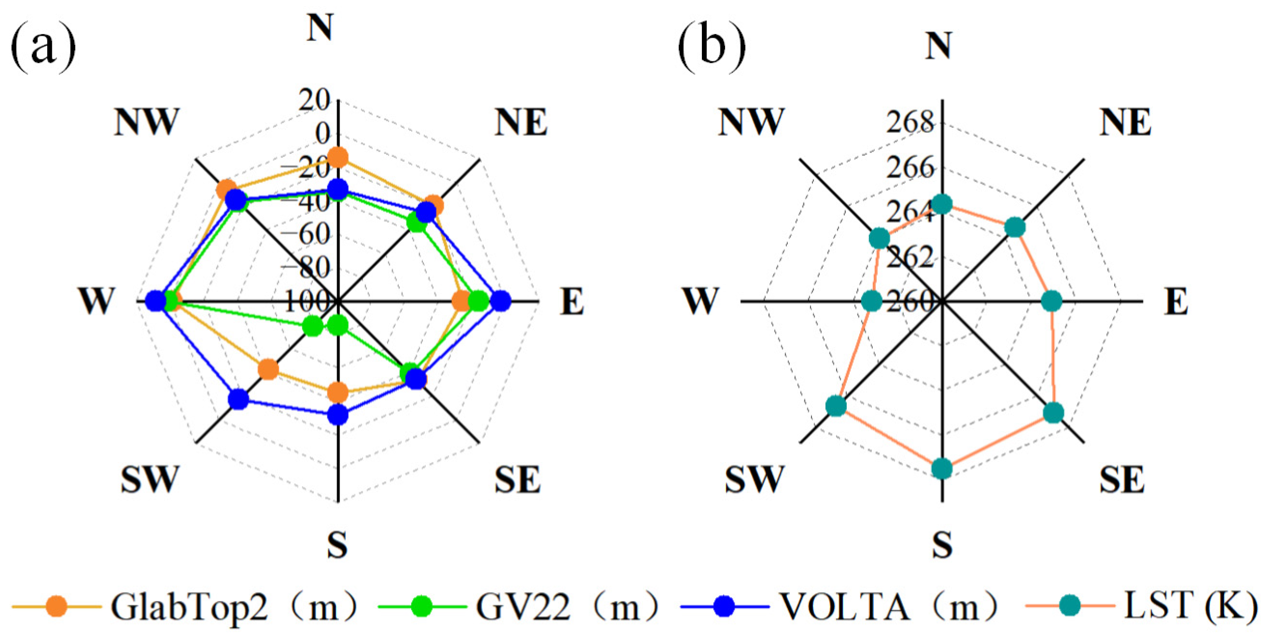
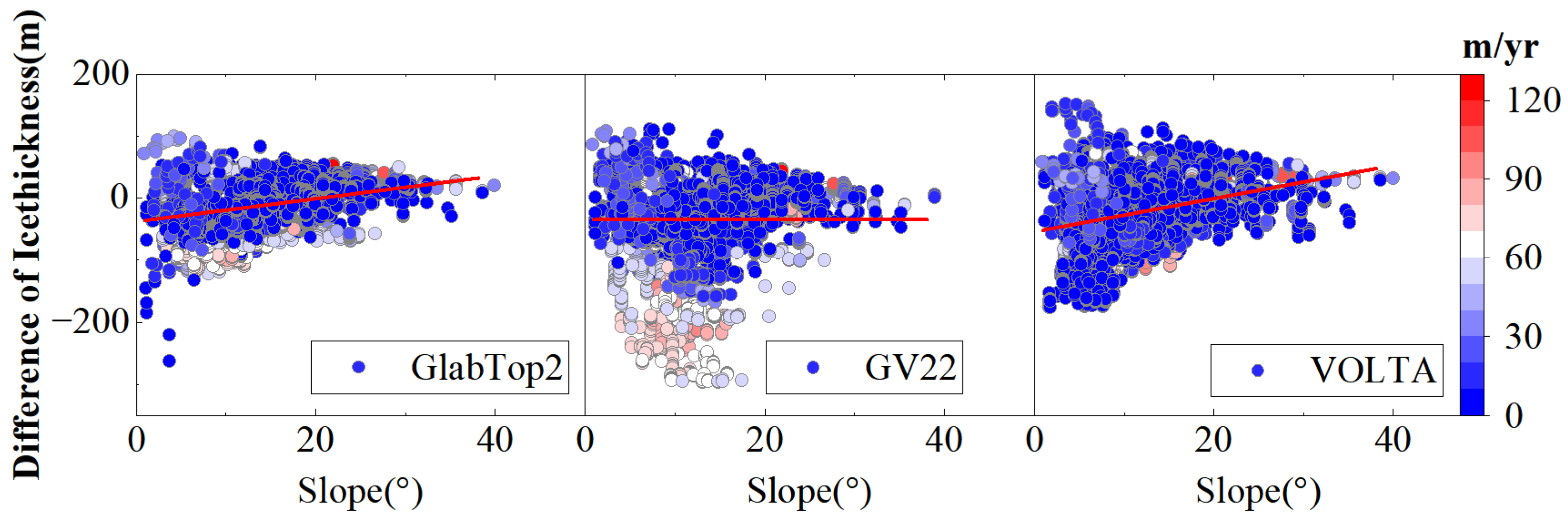
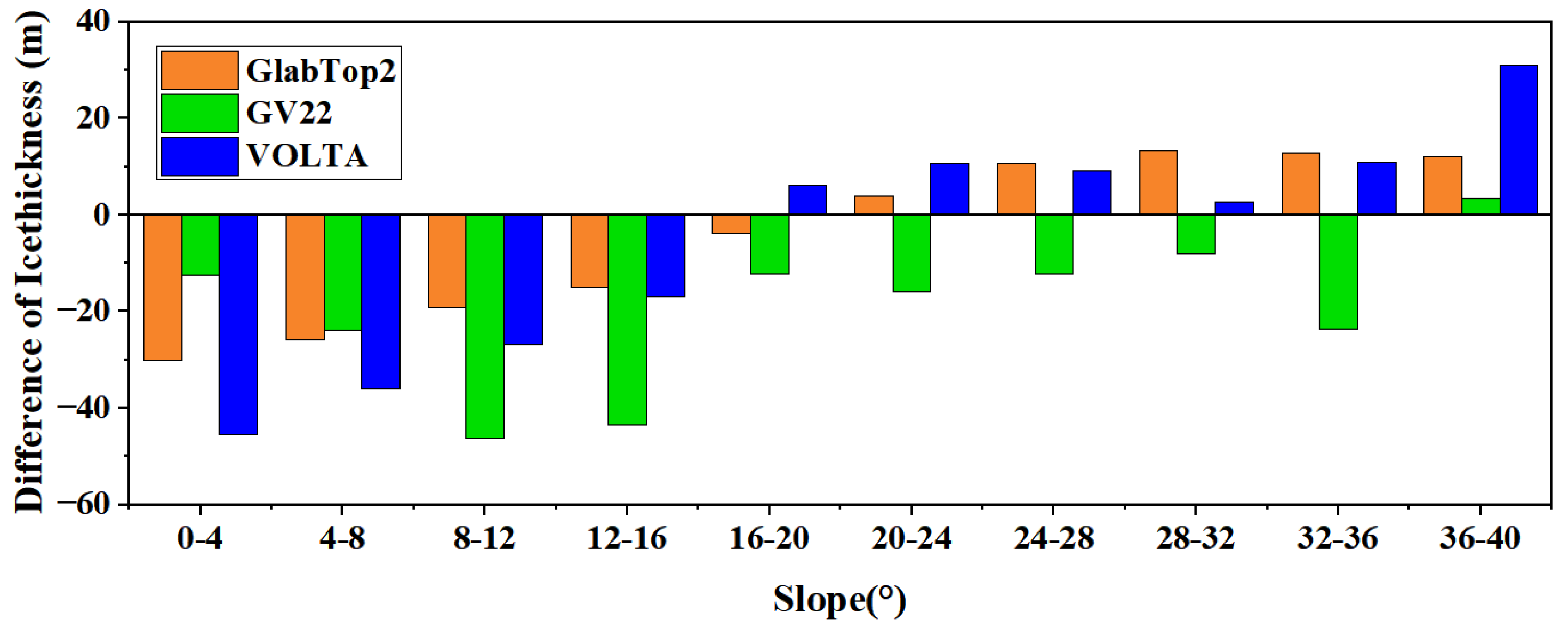
5.4. Influence of Terrain Factors on Ice Thickness Estimate

In addition, the thickness of a glacier may be influenced by topographic factors such as aspect and slope. Therefore, we calculated the bias of the three models in estimating the ice thickness in different aspects (Figure 11a). The results show that the bias of GV22 in estimating ice thickness in the S-SW aspect is significantly larger than that of other models. In the other aspects, the biases of the three models in estimating ice thickness are relatively close. This is attributed to the fact that the land surface temperature (LST) in that aspect is higher than in other aspects [40,41]. We calculated the annual mean temperature in K for the different aspects of the glacier in 2018 (Figure 11b). This indicates that solar radiation is causing glaciers to slide too quickly in this direction, resulting in a significant bias in the ice thickness estimated using the GV22 model. GV22 is not suitable for estimating glacier thickness on sunny slopes; GlabTop2 and VOLTA are not affected by aspect.

Glacier surface slope is an important input for ice thickness estimation, and we need to discuss its impact on the accuracy of ice thickness models. We extracted the simulated ice thickness and slope at the location of the GPR measurements to analyze the effect of slope on model accuracy (Figure 12). As can be seen from the figure, the deviations in ice thickness estimated using the three models are larger when the slope is less than about 20°. The deviation in ice thickness estimated using the three models decreases gradually with increasing slope. This indicates that the three models are less accurate when the slope is less than 20°. We suggest that this may be due to the gently sloping terrain. It was also shown that these three models are applicable to mountain glaciers with large slopes and are less applicable to gentle glaciers such as ice caps. In addition, the deviation in ice thickness estimated using GlabTop2 and VOLTA is concentrated in the range of −200 to 100 m, while GV22 is concentrated in the range of −300 to 100 m.

Ground slopes at GPR locations are distributed between 1 and 40°. Therefore, we calculated the mean ice thickness deviation by dividing the glacier surface slope into 4° intervals (Figure 13). As can be seen from the figure, the deviation in ice thickness estimated using GlabTop2 and VOLTA is positively correlated with the slope. The minimum ice thickness deviations simulated using GlabTop2 (−3.96 m) and VOLTA (2.73 m) correspond to slopes of 16–20° and 28–32°, respectively. The deviation of the estimated ice thickness in GV22 is −12.19 m and 3.45 m for slopes of 16–20° and 36–40°, respectively. By analyzing the results, we found that all three models provide better ice thickness estimates for slopes of 16–24°.

In addition, this study did not consider the impact of debris cover on the accuracy of the ice thickness model. Previous studies have shown that debris cover affects glacier movement, mass balance, basal sliding, etc. [55,56,57]. However, debris cover is mainly distributed on glacier tongues [58,59]. Debris cover is present on 6 (Sigonghe No. 4, Sary-tor, Heigou No. 8, Shenqi Peak, Tsentralniy tuyuksu, and Chhota Shigri) of the 10 glaciers in this study. The total debris cover area accounts for approximately 5.38% of the total area of the six glaciers [60]. The total volume of debris cover accounts for 0.09%, 0.08%, and 0.13% of the six glacier volumes estimated using GlabTop2, GV22, and VOLTA, respectively. This is not significant compared to ice thickness and ice thickness uncertainty. Therefore, debris cover has a negligible impact on model accuracy when estimating glacier thickness, but this is a very important factor when studying glacier dynamics and mass balance.

6. Conclusions

Glacier thickness is an important basis for many studies on glacier dynamics and future climate change. With the continuous increase in DEM and remote sensing data, the scientific community is using different models to estimate the volume and distribution of global glaciers. The contribution of this study is the research and analysis of widely used ice thickness models, considering that the factors affecting ice thickness inversion accuracy are unclear. We estimated the thickness of ten glaciers in HMA using three models and analyzed the accuracy and influencing factors of the results. In comparison with available GPR measurements, GlabTop2 shows a better performance than the other two models. The main factors contributing to the differences in the accuracy of the three models are glacier slope, aspect, and velocity. The three models are suitable for glaciers with slopes of 16–24°. The ice thickness accuracy of the GV22 inversion decreases significantly with increasing glacier velocity, in particular for velocities greater than 50 m/yr. In addition, sunny slopes absorb more solar radiation and have greater glacier velocity, making GV22 less accurate.

Our results show that existing glacier thickness models vary considerably in inverting the thickness of glaciers with different characteristics. In particular, the significant differences in glacier characteristics during large-scale ice volume inversion are taken into account. It is difficult to apply any single ice thickness inversion model to large-scale, high-precision ice thickness estimation. When conducting regional ice thickness inversion, choosing the appropriate ice thickness model for the study according to different glacier types and characteristics is necessary. This study may provide a reference for glaciological research.

References

1. Zou, X.; Gao, H.; Zhang, Y.; Ma, N.; Wu, J.; Bin Farhan, S. Quantifying ice storage in upper Indus river basin using ground-penetrating radar measurements and glacier bed topography model version 2. Hydrol. Process. 2021, 35, 14. [Google Scholar] [CrossRef]
2. Liang, P.-B.; Tian, L.-D. Estimation of glacier ice storage in western China constrained by field ground-penetrating Radar surveys. Adv. Clim. Change Res. 2022, 13, 359–374. [Google Scholar] [CrossRef]
3. Yao, T.D.; Thompson, L.; Yang, W.; Yu, W.S.; Gao, Y.; Guo, X.J.; Yang, X.X.; Duan, K.Q.; Zhao, H.B.; Xu, B.Q.; et al. Different glacier status with atmospheric circulations in Tibetan Plateau and surroundings. Nat. Clim. Change 2012, 2, 663–667. [Google Scholar] [CrossRef]
4. Bhambri, R.; Schmidt, S.; Chand, P.; Nusser, M.; Haritashya, U.; Sain, K.; Tiwari, S.K.; Yadav, J.S. Heterogeneity in glacier thinning and slowdown of ice movement in the Garhwal Himalaya, India. Sci. Total Environ. 2023, 875, 162625. [Google Scholar] [CrossRef]
5. Mannan Afzal, M.; Wang, X.; Sun, L.; Jiang, T.; Kong, Q.; Luo, Y. Hydrological and dynamical response of glaciers to climate change based on their dimensions in the Hunza Basin, Karakoram. J. Hydrol. 2023, 617, 128948. [Google Scholar] [CrossRef]
6. Zhang, Z.; Tao, P.; Liu, S.; Zhang, S.; Huang, D.; Hu, K.; Lu, Y. What controls the surging of Karayaylak glacier in eastern Pamir? New insights from remote sensing data. J. Hydrol. 2022, 607, 127577. [Google Scholar] [CrossRef]
7. Shugar, D.H.; Jacquemart, M.; Shean, D.; Bhushan, S.; Upadhyay, K.; Sattar, A.; Schwanghart, W.; McBride, S.; de Vries, M.V.; Mergili, M.; et al. A massive rock and ice avalanche caused the 2021 disaster at Chamoli, Indian Himalaya. Science 2021, 373, 300–306. [Google Scholar] [CrossRef]
8. Guo, R.; Jiang, L.; Xu, Z.; Li, C.; Huang, R.; Zhou, Z.; Li, T.; Liu, Y.; Wang, H.; Fan, X. Seismic and hydrological triggers for a complex cascading geohazard of the Tianmo Gully in the southeastern Tibetan Plateau. Eng. Geol. 2023, 324, 107269. [Google Scholar] [CrossRef]
9. Kraaijenbrink, P.D.A.; Bierkens, M.F.P.; Lutz, A.F.; Immerzeel, W.W. Impact of a global temperature rise of 1.5 degrees Celsius on Asia’s glaciers. Nature 2017, 549, 257–260. [Google Scholar] [CrossRef]
10. Li, F.; Maussion, F.; Wu, G.; Chen, W.; Yu, Z.; Li, Y.; Liu, G. Influence of glacier inventories on ice thickness estimates and future glacier change projections in the Tian Shan range, Central Asia. J. Glaciol. 2022, 69, 266–280. [Google Scholar] [CrossRef]
11. Sommer, C.; Fürst, J.J.; Huss, M.; Braun, M.H. Constraining regional glacier reconstructions using past ice thickness of deglaciating areas—A case study in the European Alps. Cryosphere 2023, 17, 2285–2303. [Google Scholar] [CrossRef]
12. Welty, E.; Zemp, M.; Navarro, F.; Huss, M.; Fürst, J.J.; Gärtner-Roer, I.; Landmann, J.; Machguth, H.; Naegeli, K.; Andreassen, L.M.; et al. Worldwide version-controlled database of glacier thickness observations. Earth Syst. Sci. Data 2020, 12, 3039–3055. [Google Scholar] [CrossRef]
13. Farinotti, D.; Brinkerhoff, D.J.; Clarke, G.K.C.; Fürst, J.J.; Frey, H.; Gantayat, P.; Gillet-Chaulet, F.; Girard, C.; Huss, M.; Leclercq, P.W.; et al. How accurate are estimates of glacier ice thickness? Results from ITMIX, the Ice Thickness Models Intercomparison eXperiment. Cryosphere 2017, 11, 949–970. [Google Scholar] [CrossRef]
14. Zorzut, V.; Ruiz, L.; Rivera, A.; Pitte, P.; Villalba, R.; Medrzycka, D. Slope estimation influences on ice thickness inversion models: A case study for Monte Tronador glaciers, North Patagonian Andes. J. Glaciol. 2020, 66, 996–1005. [Google Scholar] [CrossRef]
15. Farinotti, D.; Huss, M.; Fürst, J.J.; Landmann, J.; Machguth, H.; Maussion, F.; Pandit, A. A consensus estimate for the ice thickness distribution of all glaciers on Earth. Nat. Geosci. 2019, 12, 168–173. [Google Scholar] [CrossRef]
16. Frey, H.; Machguth, H.; Huss, M.; Huggel, C.; Bajracharya, S.; Bolch, T.; Kulkarni, A.; Linsbauer, A.; Salzmann, N.; Stoffel, M. Estimating the volume of glaciers in the Himalayan–Karakoram region using different methods. Cryosphere 2014, 8, 2313–2333. [Google Scholar] [CrossRef]
17. Millan, R.; Mouginot, J.; Rabatel, A.; Morlighem, M. Ice velocity and thickness of the world’s glaciers. Nat. Geosci. 2022, 15, 124–129. [Google Scholar] [CrossRef]
18. James, W.H.M.; Carrivick, J.L. Automated modelling of spatially-distributed glacier ice thickness and volume. Comput. Geosci. 2016, 92, 90–103. [Google Scholar] [CrossRef]
19. Bahr, D.B.; Pfeffer, W.T.; Kaser, G. A review of volume-area scaling of glaciers. Rev. Geophys. 2015, 53, 95–140. [Google Scholar] [CrossRef]
20. Fürst, J.J.; Gillet-Chaulet, F.; Benham, T.J.; Dowdeswell, J.A.; Grabiec, M.; Navarro, F.; Pettersson, R.; Moholdt, G.; Nuth, C.; Sass, B.; et al. Application of a two-step approach for mapping ice thickness to various glacier types on Svalbard. Cryosphere 2017, 11, 2003–2032. [Google Scholar] [CrossRef]
21. Gantayat, P.; Kulkarni, A.V.; Srinivasan, J. Estimation of ice thickness using surface velocities and slope: Case study at Gangotri Glacier, India. J. Glaciol. 2014, 60, 277–282. [Google Scholar] [CrossRef]
22. Wu, K.; Liu, S.; Zhu, Y.; Liu, Q.; Jiang, Z. Dynamics of glacier surface velocity and ice thickness for maritime glaciers in the southeastern Tibetan Plateau. J. Hydrol. 2020, 590, 125527. [Google Scholar] [CrossRef]
23. Farinotti, D.; Huss, M.; Bauder, A.; Funk, M.; Truffer, M. A method to estimate the ice volume and ice-thickness distribution of alpine glaciers. J. Glaciol. 2009, 55, 422–430. [Google Scholar] [CrossRef]
24. Maussion, F.; Butenko, A.; Champollion, N.; Dusch, M.; Eis, J.; Fourteau, K.; Gregor, P.; Jarosch, A.H.; Landmann, J.; Oesterle, F.; et al. The Open Global Glacier Model (OGGM) v1.1. Geosci. Model Dev. 2019, 12, 909–931. [Google Scholar] [CrossRef]
25. Radić, V.; Hock, R. Regional and global volumes of glaciers derived from statistical upscaling of glacier inventory data. J. Geophys. Res. 2010, 115, F01010. [Google Scholar] [CrossRef]
26. Huss, M.; Farinotti, D. Distributed ice thickness and volume of all glaciers around the globe. J. Geophys. Res. Earth Surf. 2012, 117, F04010. [Google Scholar] [CrossRef]
27. Pieczonka, T.; Bolch, T.; KrÖHnert, M.; Peters, J.; Liu, S. Glacier branch lines and glacier ice thickness estimation for debris-covered glaciers in the Central Tien Shan. J. Glaciol. 2018, 64, 835–849. [Google Scholar] [CrossRef]
28. Ramsankaran, R.; Pandit, A.; Azam, M.F. Spatially distributed ice-thickness modelling for Chhota Shigri Glacier in western Himalayas, India. Int. J. Remote Sens. 2018, 39, 3320–3343. [Google Scholar] [CrossRef]
29. Li, H.L.; Ng, F.; Li, Z.Q.; Qin, D.H.; Cheng, G.D. An extended “perfect-plasticity” method for estimating ice thickness along the flow line of mountain glaciers. J. Geophys. Res. Earth Surf. 2012, 117, 1020–1030. [Google Scholar] [CrossRef]
30. Chen, W.F.; Yao, T.D.; Zhang, G.Q.; Li, F.; Zheng, G.X.; Zhou, Y.S.; Xu, F.L. Towards ice-thickness inversion: An evaluation of global digital elevation models (DEMs) in the glacierized Tibetan Plateau. Cryosphere 2022, 16, 197–218. [Google Scholar] [CrossRef]
31. Su, F.; Pritchard, H.D.; Yao, T.; Huang, J.; Ou, T.; Meng, F.; Sun, H.; Li, Y.; Xu, B.; Zhu, M. Contrasting fate of western Third Pole’s water resources under 21st century climate change. Earth’s Future 2022, 10, e2022EF002776. [Google Scholar] [CrossRef]
32. Pfeffer, W.T.; Arendt, A.A.; Bliss, A.; Bolch, T.; Cogley, J.G.; Gardner, A.S.; Hagen, J.-O.; Hock, R.; Kaser, G.; Kienholz, C.; et al. The Randolph Glacier Inventory: A globally complete inventory of glaciers. J. Glaciol. 2014, 60, 537–552. [Google Scholar] [CrossRef]
33. Zhan, J.; Shi, H.; Wang, Y.; Yao, Y. Complex principal component analysis of mass balance changes on the Qinghai–Tibetan Plateau. Cryosphere 2017, 11, 1487–1499. [Google Scholar] [CrossRef]
34. Farinotti, D.; Brinkerhoff, D.J.; Furst, J.J.; Gantayat, P.; Gillet-Chaulet, F.; Huss, M.; Leclercq, P.W.; Maurer, H.; Morlighem, M.; Pandit, A.; et al. Results from the Ice Thickness Models Intercomparison eXperiment Phase 2 (ITMIX2). Front. Earth Sci 2021, 8, 21. [Google Scholar] [CrossRef]
35. Azam, M.F.; Wagnon, P.; Ramanathan, A.; Vincent, C.; Sharma, P.; Arnaud, Y.; Linda, A.; Pottakkal, J.G.; Chevallier, P.; Singh, V.B. From balance to imbalance: A shift in the dynamic behaviour of Chhota Shigri glacier, western Himalaya, India. J. Glaciol. 2012, 58, 315–324. [Google Scholar] [CrossRef]
36. Reuter, H.I.; Nelson, A.; Jarvis, A. An evaluation of void-filling interpolation methods for SRTM data. Int. J. Geogr. Inf. Sci. 2007, 21, 983–1008. [Google Scholar] [CrossRef]
37. González-Moradas, M.d.R.; Viveen, W. Evaluation of ASTER GDEM2, SRTMv3.0, ALOS AW3D30 and TanDEM-X DEMs for the Peruvian Andes against highly accurate GNSS ground control points and geomorphological-hydrological metrics. Remote Sens. Environ. 2020, 237, 111509. [Google Scholar] [CrossRef]
38. Hawker, L.; Uhe, P.; Paulo, L.; Sosa, J.; Savage, J.; Sampson, C.; Neal, J. A 30 m global map of elevation with forests and buildings removed. Environ. Res. Lett. 2022, 17, 024016. [Google Scholar] [CrossRef]
39. Becek, K.; Koppe, W.; Kutoğlu, Ş. Evaluation of Vertical Accuracy of the WorldDEM™ Using the Runway Method. Remote Sens. 2016, 8, 934. [Google Scholar] [CrossRef]
40. Zhang, X.; Zhou, J.; Göttsche, F.M.; Zhan, W.; Liu, S.; Cao, R. A Method Based on Temporal Component Decomposition for Estimating 1-km All-Weather Land Surface Temperature by Merging Satellite Thermal Infrared and Passive Microwave Observations. IEEE Trans. Geosci. Remote Sens. 2019, 57, 4670–4691. [Google Scholar] [CrossRef]
41. Zhang, X.; Zhou, J.; Liang, S.; Wang, D. A practical reanalysis data and thermal infrared remote sensing data merging (RTM) method for reconstruction of a 1-km all-weather land surface temperature. Remote Sens. Environ. 2021, 260, 112437. [Google Scholar] [CrossRef]
42. Millan, R.; Mouginot, J.; Rabatel, A.; Jeong, S.; Cusicanqui, D.; Derkacheva, A.; Chekki, M. Mapping Surface Flow Velocity of Glaciers at Regional Scale Using a Multiple Sensors Approach. Remote Sens. 2019, 11, 2498. [Google Scholar] [CrossRef]
43. Linsbauer, A.; Paul, F.; Hoelzle, M.; Frey, H.; Haeberli, W. The Swiss Alps Without Glaciers—A GIS-based Modelling Approach for Reconstruction of Glacier Beds. In Geomorphometry 2009 International Conference; Department of Geography, University of Zurich: Zurich, Switzerland, 2009. [Google Scholar]
44. Haeberli, W.; Hoelzle, M. Application of inventory data for estimating characteristics of and regional climate-change effects on mountain glaciers: A pilot study with the European Alps. Ann. Glaciol. 1995, 21, 206–212. [Google Scholar] [CrossRef]
45. Gharehchahi, S.; James, W.H.M.; Bhardwaj, A.; Jensen, J.L.R.; Sam, L.; Ballinger, T.J.; Butler, D.R. Glacier Ice Thickness Estimation and Future Lake Formation in Swiss Southwestern Alps—The Upper Rhône Catchment: A VOLTA Application. Remote Sens. 2020, 12, 3443. [Google Scholar] [CrossRef]
46. Driedger, C.L.; Kennard, P.M. Glacier Volume Estimation on Cascade Volcanoes: An Analysis and Comparison with Other Methods. Ann. Glaciol. 1986, 8, 59–64. [Google Scholar] [CrossRef]
47. Lei, Y.; Gardner, A.; Agram, P. Autonomous Repeat Image Feature Tracking (autoRIFT) and Its Application for Tracking Ice Displacement. Remote Sens. 2021, 13, 749. [Google Scholar] [CrossRef]
48. Zhou, Y.; Chen, J.; Cheng, X. Glacier Velocity Changes in the Himalayas in Relation to Ice Mass Balance. Remote Sens. 2021, 13, 3825. [Google Scholar] [CrossRef]
49. Glen, J.W. The creep of polycrystalline ice. Proc. R. Soc. Lond. Ser. A. Math. Phys. Sci. 1955, 228, 519–538. [Google Scholar]
50. Höhle, J.; Höhle, M. Accuracy assessment of digital elevation models by means of robust statistical methods. ISPRS J. Photogramm. Remote Sens. 2009, 64, 398–406. [Google Scholar] [CrossRef]
51. Muhuri, A.; Gascoin, S.; Menzel, L.; Kostadinov, T.S.; Harpold, A.A.; Sanmiguel-Vallelado, A.; Lopez-Moreno, J.I. Performance Assessment of Optical Satellite-Based Operational Snow Cover Monitoring Algorithms in Forested Landscapes. IEEE J. Sel. Top. Appl. Earth Obs. Remote Sens. 2021, 14, 7159–7178. [Google Scholar] [CrossRef]
52. Chymyrov, A. Comparison of different DEMs for hydrological studies in the mountainous areas. Egypt. J. Remote Sens. Space Sci. 2021, 24, 587–594. [Google Scholar] [CrossRef]
53. Wang, P.Y.; Li, Z.Q.; Wang, W.B.; Li, H.L.; Wang, F.T. Glacier Volume Calculation from Ice-Thickness Data for Mountain Glaciers-A Case Study of Glacier No. 4 of Sigong River over Mt. Bogda, Eastern Tianshan, Central Asia. J. Earth Sci. 2014, 25, 371–378. [Google Scholar] [CrossRef]
54. Patel, A.; Goswami, A.; Dharpure, J.K.; Sharma, P.; Patel, L.K.; Thamban, M. Monitoring glacier characteristics and their mass balance using a multidimensional approach over the glaciers of the Chandra basin, western Himalaya. Hydrol. Sci. J. 2022, 67, 419–435. [Google Scholar] [CrossRef]
55. Chen, F.; Wang, J.; Li, B.; Yang, A.; Zhang, M. Spatial variability in melting on Himalayan debris-covered glaciers from 2000 to 2013. Remote Sens. Environ. 2023, 291, 113560. [Google Scholar] [CrossRef]
56. Compagno, L.; Huss, M.; Miles, E.S.; McCarthy, M.J.; Zekollari, H.; Dehecq, A.; Pellicciotti, F.; Farinotti, D. Modelling supraglacial debris-cover evolution from the single-glacier to the regional scale: An application to High Mountain Asia. Cryosphere 2022, 16, 1697–1718. [Google Scholar] [CrossRef]
57. Iverson, N.R.; Helanow, C.; Zoet, L.K. Debris-bed friction during glacier sliding with ice–bed separation. Ann. Glaciol. 2020, 60, 30–36. [Google Scholar] [CrossRef]
58. Shukla, A.; Garg, P.K. Evolution of a debris-covered glacier in the western Himalaya during the last four decades (1971–2016): A multiparametric assessment using remote sensing and field observations. Geomorphology 2019, 341, 1–14. [Google Scholar] [CrossRef]
59. Neckel, N.; Loibl, D.; Rankl, M. Recent slowdown and thinning of debris-covered glaciers in south-eastern Tibet. Earth Planet. Sci. Lett. 2017, 464, 95–102. [Google Scholar] [CrossRef]
60. Rounce, D.R.; Hock, R.; McNabb, R.W.; Millan, R.; Sommer, C.; Braun, M.H.; Malz, P.; Maussion, F.; Mouginot, J.; Seehaus, T.C.; et al. Distributed Global Debris Thickness Estimates Reveal Debris Significantly Impacts Glacier Mass Balance. Geophys. Res. Lett. 2021, 48, 12. [Google Scholar] [CrossRef]
Figure 1. Glacier distribution of the HMA. The blue and gray polygons indicate glacier and subregional boundaries, respectively. Glaciers and subregional boundaries are from RGI-6.0. Red dots indicate the location of glaciers for the experiment.
Remotesensing 15 05378 g001
Figure 2. Ice thickness distribution of Chhota Shigri glacier modeled using GlabTop2 (a), GV22 (b), and VOLTA (c). CS1-5 in the figure show the position of the GPR measurement line, from which it can be seen whether the measured thickness corresponds to the estimated thickness.
Remotesensing 15 05378 g002
Figure 3. Distribution of glacier thicknesses estimated using different models. The color of the dots indicates the ice thickness measured using GPR.
Remotesensing 15 05378 g003
Figure 4. Ice thickness of Chhota Shigri glacier cross-section as measured using GPR and simulated using different models. CS1-5 in the figures indicates the cross-section in Figure 2.
Remotesensing 15 05378 g004
Figure 5. Comparative analysis of glacier thicknesses from different models and GPR measurements. The last one is a comparison of the overall 10 glaciers with the GPR-measured ice thicknesses. The numbers in the graph correspond to the IDs in Table 1.
Remotesensing 15 05378 g005
Figure 6. The accuracy of the estimated thickness of each glacier under different evaluation metrics. The first to third rows are VOLTA, GV22, and GlabTop2 in that order.
Remotesensing 15 05378 g006
Figure 7. Comparison and analysis of the estimated ice thicknesses in this study with Farinotti et al. and GPR [12,15,35]. The first four columns of bars show the maximum ice thickness of the glacier, and the last four columns show the average thickness of the glacier. Total represents the average ice thickness of 10 glaciers at GPR points.
Remotesensing 15 05378 g007
Figure 8. The trend in RMSE values of glacier thickness as the value of GlabTop2 model parameter f (shape factor) increases. The legend on the right provides the optimal shape factor for each glacier.
Remotesensing 15 05378 g008
Figure 9. The sensitivity of ice thickness is estimated using different models to different variables. (af) Ice thickness corresponds to different values of creep parameters, surface velocity, shape factor, ice density, surface slope, and basal shear stress.
Remotesensing 15 05378 g009
Figure 10. Deviations and trends in ice thickness are estimated using the three models with increasing surface velocity. From top to bottom are the GV22, GlabTop2, and VOLTA models. The black dashed line indicates the trend of ice thickness deviation with surface velocity. K1 and K2 represent the slopes of the black dotted lines for speeds less than 50 m/yr and greater than 50 m/yr, respectively.
Remotesensing 15 05378 g010
Figure 11. Effect of aspect on the accuracy of ice thickness inversion. (a) Deviations of the three models in estimating ice thickness at different aspects. (b) LST for different aspects.
Remotesensing 15 05378 g011
Figure 12. Deviations of three ice thickness model inversions for different surface slopes. The color of the dot indicates the velocity.
Remotesensing 15 05378 g012
Figure 13. Deviation in ice thickness estimated using the three models after dividing the surface slope at 4° intervals.
Remotesensing 15 05378 g013