Abstract
The continuously improving performance of mass-market global navigation satellite system (GNSS) chipsets is enabling the prospect of high-precision GNSS positioning for smartphones. Nevertheless, a substantial portion of Android smartphones lack the capability to access raw carrier phase observations. Therefore, this paper introduces a precise code positioning (PCP) method, which utilizes Doppler-smoothed pseudo-range and inter-satellite single-difference methods. For the first time, the results of a quality investigation involving BDS-3 B1C/B2a/B1I, GPS L1/L5, and Galileo E1/E5a observed using smartphones are presented. The results indicated that Xiaomi 11 Lite (Mi11) exhibited a superior satellite data decoding performance compared to Huawei P40 (HP40), but it lagged behind HP40 in terms of satellite tracking. In the static open-sky scenario, the carrier-to-noise ratio (CNR) values were mostly above 25 dB-Hz. Additionally, for B1C/B1I/L1/E1, they were approximately 8 dB-Hz higher than those for B2a/L5/E5a. Second, various PCP models were developed to address ionospheric delay. These models include the IF-P models, which combine traditional dual-frequency IF pseudo-ranges with single-frequency ionosphere-corrected pseudo-ranges using precise ionospheric products, and IFUC models, which rely solely on single-frequency ionosphere-corrected pseudo-ranges. Finally, static and dynamic tests were conducted using datasets collected from various real-world scenarios. The static tests demonstrated that the PCP models could achieve sub-meter-level accuracy in the east (E) and north (N) directions, while achieving meter-level accuracy in the upward (U) direction. Numerically, the root mean square error (RMSE) improvement percentages were approximately 93.8%, 75%, and 82.8% for HP40 in the E, N, and U directions, respectively, in both open-sky and complex scenarios compared to single-point positioning (SPP). In the open-sky scenario, Mi11 showed an average increase of about 85.6%, 87%, and 16% in the E, N, and U directions, respectively, compared to SPP. In complex scenarios, Mi11 exhibited an average increase of roughly 68%, 75.9%, and 90% in the E, N, and U directions, respectively, compared to SPP. Dynamic tests showed that the PCP models only provided an improvement of approximately 10% in the horizontal plane or U direction compared to SPP. The triple-frequency IFUC (IFUC123) model outperforms others due to its lower noise and utilization of multi-frequency pseudo-ranges. The PCP models can enhance smartphone positioning accuracy.
1. Introduction
Nowadays, there is a rising demand among the general public for location-based services (LBSs) during their daily journeys. As a result, there is a growing need for high-precision positioning capabilities in mass-market smartphones. In 2016, Google made an announcement that it would provide access to raw GNSS measurements through the Android Nougat operating system [1]. Since then, a multitude of studies have been carried out to improve the performance of GNSS positioning when utilizing mass-market smartphones [2,3,4].
Banville and Diggelen [5] conducted an analysis of the quality of GPS single-frequency (SF) observations using the Galaxy S7. Their findings revealed that the Galaxy S7 exhibited notably high pseudo-range noise levels, which imposed limitations on positioning accuracy within the meter-level range. Zhang et al. [6] conducted an examination of the quality of raw GNSS measurements gathered using the Huawei P9. Their findings indicated that the average carrier-to-noise ratio (CNR) typically reached 25 dB-Hz, while pseudo-range noise levels ranged between 8 and 12 m. Zhang et al. [7] introduced an algorithm based on the time-differenced carrier phase (TDCP) filter, which achieved meter-level positioning accuracy. Their research particularly highlighted the significance of carrier-to-noise ratio (CNR) values in determining the quality of smartphone measurements. References [8,9,10,11] concluded that the traditional elevation-weight method is not suitable for smartphones, while the CNR-weighted approach was deemed more suitable and effective.
Precise point positioning (PPP) is one of the methods employed to attain high-precision positioning, and several research studies have been conducted on implementing PPP with smartphones [12,13]. Gill et al. [14] utilized Global Ionospheric Map (GIM) products to correct for ionospheric delays in measurements collected with the Nexus 9, thereby achieving sub-meter-level positioning accuracy through GPS single-frequency (SF) PPP. In 2018, Xiaomi 8 made its debut as the world’s first smartphone capable of observing dual-frequency (DF) raw GNSS measurements [15]. Since then, researchers have embarked on comprehensive investigations into the positioning performance of dual-frequency GNSS smartphones. In studies [16,17], it was revealed that incorporating L5/E5a measurements can significantly enhance positioning accuracy. Robustelli et al. [18] conducted an assessment of code measurements, considering pseudo-range noise and multi-path errors. Their results indicated that GPS satellites tend to exhibit more multi-path errors when compared to Galileo satellites, and that L5/E5a signals demonstrate higher quality than the L1/E1 signals.
Elmezayen et al. [19] conducted a study on dual-frequency (DF) ionosphere-free (IF) PPP in an open-sky environment, utilizing GNSS measurements from the Xiaomi 8 smartphone. Their results showed that DF IF PPP was capable of achieving sub-meter-level positioning accuracy. Wu et al. [20] conducted an investigation into the DF PPP performance of the Xiaomi 8 smartphone in both static and dynamic scenarios. Their experimental results indicated that in static scenarios, the convergence accuracy could reach sub-meter levels, but it required a lengthy convergence time of up to 3 h. In dynamic scenarios, due to the limited number of available satellites, positioning errors reached several meters or even tens of meters. Aggrey et al. [21] conducted an investigation into the precision limits of SF and DF PPP using smartphones in a static open-sky environment. Their experimental results indicated that the convergence accuracy showed slight variations among different smartphones, with sub-meter-level precision attainable. However, there were notable differences in convergence times observed among the various smartphones. Psychas et al. [22] demonstrated that multi-GNSS DF positioning performs better than SF positioning. In studies [23,24,25], researchers conducted an analysis of the quality of raw GNSS measurements and performed PPP experiments in both static and dynamic scenarios. Their results indicated that smartphones can achieve sub-meter positioning accuracy in static open-sky environments and meter-level positioning accuracy in dynamic scenarios.
In addition to absolute positioning PPP methods, there is also research on relative positioning methods, with real-time kinematics (RTK) being a primary technique. There have also been studies focusing on RTK applications for smartphones [26,27,28]. In studies [29,30], experiments were conducted to validate the performance of smartphone RTK, and the results demonstrated that it can achieve meter-level positioning accuracy. Geng et al. [31] introduced a robust RTK scheme utilizing sliding window-based factor graph optimization, which achieved sub-meter-level positioning accuracy in open-sky urban areas and meter-level accuracy in complex urban environments. Jiang et al. [32] introduced an enhanced ambiguity resolution algorithm aimed at achieving centimeter-level RTK positioning. Tao et al. [33] introduced a multi-GNSS RTK positioning method tailored for smartphones, specifically suitable for real kinematic conditions. Their experimental results showed that DF RTK could attain meter-level accuracy. They concluded that smartphones hold significant potential for achieving high-precision navigation and positioning in real urban environments.
In the previously mentioned studies, both PPP and RTK, which rely on carrier phase observations, were utilized to achieve high-precision GNSS positioning with smartphones. However, it is worth noting that only a small number of smartphones can output the AccumulatedDeltaRangeMeters data, which is essential for obtaining carrier phase measurements [34]. This results in the limited applicability of PPP and RTK techniques for widespread use in smartphones among the general public. Additionally, the vast majority of smartphones can now access dual- or even triple-frequency pseudo-range observation data. However, traditional single-point positioning (SPP) cannot fully harness the raw smartphone GNSS observation data. Therefore, multi-frequency ionosphere-free precise code pseudo-range positioning suitable for smartphones holds substantial research significance and practical value in enhancing smartphone GNSS positioning.
The main contributions of this study can be summarized as follows. Firstly, an analysis was conducted on BDS-3 B1C/B2a/B1I, GPS L1/L5, and Galileo E1/E5a measurements collected in various scenarios using Xiaomi 11 Lite (Mi11) and Huawei P40 (HP40) smartphones. Second, various PCP models were derived. Third, the performance of these positioning methods was assessed using real-world datasets obtained from various scenarios. Finally, conclusions based on the findings in this study are provided.
2. Data Quality Characteristic Analysis
In this section, we followed the method outlined by Zangenehnejad and Gao [2] to develop an Android application capable of analyzing the full-frequency signal of all satellites observed using smartphones. Real-world datasets were used to evaluate the quality of the BDS-3 B1C/B2a/B1I, GPS L1/L5, and Galileo E1/E5a signals. Data collection was carried out using two smartphones, namely, a Huawei P40 (HP40) and a Xiaomi 11 Lite (Mi11).
2.1. Data Description
We collected datasets at a 1 Hz sampling rate in both static and dynamic scenarios, each of which featured two distinct environments. In the static scenario, we collected observations for approximately 2 h on 13 June 2023, encompassing both open-sky and complex environments. In the dynamic scenario, we gathered observations in both typical and complex urban environments on 14 June 2023, with a data collection time of roughly 30 min. All of these datasets were obtained at the China University of Mining and Technology in Xuzhou, China. It is important to emphasize that HP40 lacks the ability to output ReceivedSvTimeNanos data for B1C and B2a, which is essential for pseudo-range calculation. Conversely, Mi11 lacks the ability to output AccumulatedDeltaRangeMeters data for all frequencies, which is crucial for carrier-phase calculation. Consequently, pseudo-range data for B1C and B2a in the HP40 could not be obtained.
Figure 1a illustrates the locations of the static data. On the left, the smartphones were located in a challenging environment surrounded by trees, while on the right, they were situated in an open-sky environment atop a building. Figure 1b shows the trajectories of the dynamic data. In the figure, the red track indicates a typical urban environment with a wide road and trees on both sides, although the obstruction is not extensive. On the other hand, the green track represents a complex urban environment with narrow roads, tightly sheltered trees, and buildings nearby. Throughout the experiments, reference positions were provided by the geodetic receiver, namely the CHC i70.
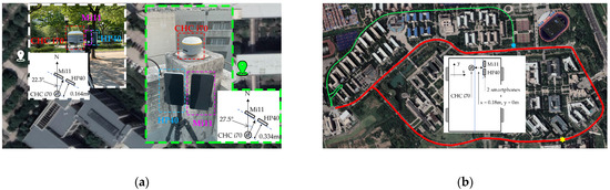
Figure 1.
Information on dataset collection. (a) Static dataset collection environment and relative positions of smartphones and geodetic receiver. (b) Trajectory of dynamic dataset collections and relative positions of two smartphones and geodetic receiver.
2.2. Satellite Visibility
Figure 2 provides a comparison of the number of visible satellites in each constellation and frequency as observed using the HP40 and Mi11 GNSS receivers. Specifically, “B1C&B2a” indicates the satellites observed using smartphones with B1C and B2a signals, and “B1C&B2a&B1I” includes the satellites observed with B1C, B2a, and B1I data. Similarly, “L1&L5” and “E1&E5a” follow the same conventions as described above.
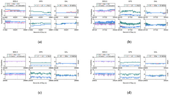
Figure 2.
Number of visible satellites for smartphone multi-GNSS. (a) Number of satellites for HP40 and Mi11 in the static open-sky scenario; (b) number of satellites for HP40 and Mi11 in the static complex scenario; (c) number of satellites for HP40 and Mi11 in the dynamic typical urban scenario; (d) number of satellites for HP40 and Mi11 in the dynamic complex urban scenario.
Figure 2 clearly shows that the number of visible GPS L5 satellites was consistently lower than four for the HP40. By contrast, Mi11 observed more than four GPS L5 satellites only in the static open-sky scenario. In all other scenarios, except for the static open-sky scenario, Mi11 observed fewer than four satellites for most of the observation epochs.
In the static open-sky scenario, HP40 observed approximately seven to eight BDS-3 B1C satellites, seven to ten B2a satellites, nine to eleven B1I satellites, six to seven satellites for B1C&B2a, and six to seven satellites for B1C&B2a&B1I. On the other hand, Mi11 recorded eight to eleven satellites for B1C, B2a, B1C&B2a, and B1C&B2a&B1I, and ten to fifteen satellites for B1I. It is worth noting that in two epochs, Mi11 did not detect any B1I or B1C&B2a&B1I satellites. For GPS, the HP40 typically observed five to eight L1 satellites, one to two L5 satellites, and one to two L1&L5 satellites. By contrast, Mi11 observed six to ten L1 satellites and three to seven L5 satellites. Regarding Galileo, HP40 typically observed five to seven E1 satellites and six to eleven E5a satellites. Meanwhile, Mi11 observed six to eleven Galileo satellites. Table 1 presents the average number of visible satellites across various frequencies for both HP40 and Mi11 in the static open-sky scenario. Figure 2 and Table 1 clearly indicate that HP40’s performance in decoding satellite data was inferior when compared to Mi11. This difference in performance could be attributed to the fact that Mi11, equipped with a new-generation chip, was released in March 2021, by which time the BDS-3 system had already been operating successfully. Notably, the Mi11 has the capability to obtain C59 and C60 B1I observations, which HP40 cannot access.

Table 1.
Average numbers of satellites in each frequency for smartphones in the static open-sky scenario.
In the static complex scenario, when compared to the static open-sky scenario, HP40 consistently maintained the same number of visible satellites for BDS-3, GPS, and Galileo. However, Mi11 experienced a decrease of one to two satellites. It is worth noting that the fluctuation range of the number of visible satellites for each constellation is greater than that in the static open-sky scenario. In the dynamic scenario, HP40 witnessed a reduction of one satellite for BDS-3, GPS, and Galileo compared to the static open-sky scenario, whereas Mi11 experienced a more substantial decrease of two to three satellites. Notably, the fluctuation range of the number of visible satellites for each constellation remained the same as in the static open-sky scenario for HP40, but it was larger than that in the static open-sky scenario and smaller than that in the static complex scenario for Mi11. This suggests that Mi11’s performance in tracking satellites may be weaker compared to HP40 in certain scenarios.
2.3. Signal Power
The CNR represents the ratio of signal power to noise in the process of receiving the signal. The CNR value serves as an indicator of the signal noise level of observation satellites during experimental measurements. A lower CNR value indicates poorer observation quality.
Table 2 presents the average CNR values in dB-Hz for each frequency of both HP40 and Mi11 in the static open-sky scenario. Figure 3 illustrates a comparison of the CNR for each frequency in smartphone GNSS observations. In general, the CNR for multi-GNSS signals fell within the range of 25–45 dB-Hz. Specifically, for HP40, the CNR of the B2a/L5/E5a signal was approximately 10 dB-Hz lower than that of B1C/B1I/L1/E1, whereas for Mi11, it was approximately 6 dB-Hz lower. In the static complex scenario, the CNR was 4 dB-Hz lower than in the static open-sky scenario for HP40 and 2 dB-Hz lower for Mi11. In the dynamic typical urban scenario, both HP40 and Mi11 exhibited a CNR approximately 2 dB-Hz lower than in the static open-sky scenario. Additionally, in the dynamic complex urban scenario, the CNR was approximately 2 dB-Hz lower than in the dynamic typical urban scenario.
Table 2.
The average CNR values in each frequency for smartphones in the static open-sky scenario.
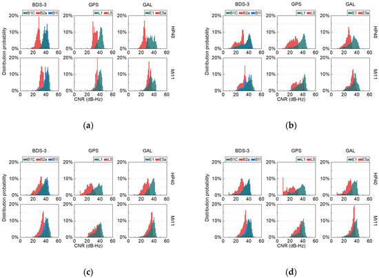
Figure 3.
Distribution of the CNR for smartphones’ multi-GNSS. (a) CNR distribution for HP40 and Mi11 in the static open-sky scenario. (b) CNR distribution for HP40 and Mi11 in the static complex scenario. (c) CNR distribution for HP40 and Mi11 in the dynamic typical urban scenario. (d) CNR distribution for HP40 and Mi11 in the dynamic complex urban scenario.
As seen in Figure 3, in the static open-sky scenario, the proportion of satellites with a CNR below 25 dB-Hz was very small. Specifically, for Mi11, 40–70% of the BDS-3 B1C/B1I and GPS L1 satellites had a CNR exceeding 40 dB-Hz, while the percentages for HP40 were 39-65%. Approximately 25% of Galileo E1 satellites had a CNR exceeding 40 dB-Hz. Regarding the second-frequency signals, for Mi11, only approximately 8% of GPS L5 satellites had a CNR exceeding 40 dB-Hz, and the majority of them were around 36 dB-Hz. Additionally, less than 1% of BDS-3 B2a satellites had a CNR exceeding 40 dB-Hz, with most of them around 33 dB-Hz. As for Mi11’s E5a CNR, it was mainly distributed around 32 dB-Hz. However, for HP40, there were no second-frequency satellites with CNRs exceeding 40 dB-Hz. For HP40, the CNR value for B2a was mainly distributed around 29 dB-Hz, while it was around 31 dB-Hz for L5 and around 25 dB-Hz for E5a.
However, in the static complex and dynamic scenarios, the CNR decreased due to interference from the surrounding environment. When the CNR of smartphone GNSS observations drops below 25 dB-Hz, it can significantly increase the occurrence of gross errors. In such cases, if there is a sufficient number of visible satellites, it is crucial to take measures to avoid using observations with CNRs below 25 dB-Hz, so as to minimize abnormal positioning results.
Figure 4 illustrates that as elevation increased, there was no significant increase in the CNR. Therefore, the relationship between the CNR and elevation does not appear to be closely correlated. As mentioned in the Introduction section, there is substantial research indicating a strong connection between smartphone GNSS observation quality and the CNR. Hence, it can be inferred that satellite elevation does not significantly affect smartphone GNSS observation quality.
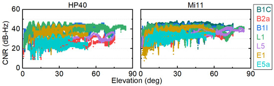
Figure 4.
The distribution of the CNR of smartphones (HP40 on the left, Mi11 on the right) at various frequencies under different elevations in the static open-sky scenario. Each color corresponds to a specific frequency, as explained in the figure legend.
2.4. Observation Noise of Pseudo-Range
The noise of the pseudo-range was calculated based on the third-derivative approach. The third-derivative approach is similar to a high-pass filter, which excludes the low-frequency measurement delays while preserving the high-frequency noise. The noise calculation equation is as follows [35]:
where is the noise of the pseudo-range; is the pseudo-range measurement at epoch ; is the time interval; and is the normalization factor according to the law of error propagation. Note that the approach requires continuous observations and high sampling rates.
Table 3 shows the results of pseudo-range noise measured in meters. It is important to highlight that the observed noise values for each frequency appear abnormally large. This anomaly arises because of discontinuities in the code clock. The data acquisition software no longer aligns the pseudo-range generation time with the first available epoch; instead, it uses the FullBiasNanos parameter epoch-by-epoch. The FullBiasNanos parameter, which is used for pseudo-range calculations, represents the deviation between the receiver hardware clock and GPST (GPS time), but it introduces a jump of approximately 256 ns at regular intervals [36]. This jump disrupts the continuity of the pseudo-range clock. The third-order derivative method, used for noise calculation, cannot effectively eliminate the influence of high-frequency noise caused by these clock jumps, nor can it differentiate between clock noise and electronic thermal noise [37]. Consequently, this leads to excessively large calculated noise values. The pseudo-range noise obtained through this method is highly inaccurate and can only serve as a reference under similar conditions. One observation from the data is that B1C/E1 signals exhibited stronger resistance to interference compared to B2a/E5a, and within the GPS signals, L5 demonstrated greater anti-interference capabilities than L1.
Table 3.
Smartphone multi-frequency pseudo-range noise STD in the static open-sky scenario.
3. Methodology for Precise Code Positioning
The functional models for precise code positioning are outlined in this section, described based on the general observation model. To simplify, we designated the three frequencies as numbers 1, 2, and 3. The specific frequencies indicated by the numbers are shown in Table 4, and the values in parentheses are in MHz. It is important to note that, in the case of BDS-3, the IF combination of B1C/B1I introduces a significantly higher noise amplification factor compared to that of B2a/B1I [38]. Therefore, the IF13 combination in the experiment employs the IF combination of B2a/B1I. In the context of BDS-3, this means that the IF combination used is IF1223, but for simplicity, it is still referred to as IF1213 in the model derivation below.
Table 4.
BDS-3/GPS/Galileo frequency numbers.
3.1. General Code Observation Model
The code observation on a single frequency is as follows [39]:
where the superscripts and , and subscript represent the satellite, constellation, and receiver, respectively; is the code observed-minus-computed values; j denotes the frequency (j = 1, 2, 3); is the unit vector of direction; represents the vector of position correction to the priori position; and and indicate the receiver and satellite clock offsets, respectively. is the ionospheric factor; f indicates the frequency; and denotes the slant ionospheric delay at the first frequency. Furthermore, is the zenith wet tropospheric delay. The tropospheric delay can be divided into two parts, namely, the hydrostatic delay part and the wet delay part, both of which are able to be expressed as the product of a zenith path delay and a mapping function; the zenith dry delay can be calculated using the Saastamoinen model [40,41]. The parameters and are the code hardware delays from the receiver side and satellite side, respectively. represents the measurement noise of the code including multipath errors.
Moreover, the following variables are defined herein for ease of expression:
where and are the frequency (); and represent the coefficients of the combination; and represent the differential code bias (DCB) of the satellite.
The GNSS precise satellite clock products, which can be downloaded from ftp://igs.gnsswhu.cn/pub/gps/products/mgex/ (accessed on 1 July 2023) [42], are based on the dual frequency IF combined code and phase observations solved for the first and second frequencies (e.g., BDS B1I/B3I, GPS L1/L2, and Galileo E1/E5a) [43]. Although some GPS satellites have the time-varying part of the carrier phase delay [44], its influence can be ignored in the code observation equation. Thus, the precise satellite clock, which is a linear combination of the code hardware bias, is expressed as follows [45]:
After the correction of the precision satellite clock product and the satellite DCB product, Equation (2) can be expressed as follows:
where represents the receiver-side clock offsets.
3.2. Doppler-Smoothed-Code Method
To reduce pseudo-range noise and address code multipath effects, a practical approach is to use carrier-smoothed code (CSC) or Doppler-smoothed code (DSC). However, CSC is not suitable for smartphones due to several reasons. Firstly, the low-cost antenna on smartphones often results in numerous cycle-slips in the observed carrier phase observations [35,46]. Secondly, as mentioned earlier, most smartphones cannot obtain carrier phase observations. The DSC method is expressed as follows [47]:
where is the smoothed pseudo-range, represents the epoch, is the interval between and the epoch, and is the Doppler observation. needs to satisfy the following condition:
where represents the maximum smoothing window and is device dependent, typically falling within the range of 50 to 100 epochs. It is important to note that when employing the DSC method, data preprocessing is a crucial initial step to eliminate outliers. If outliers are detected, the smoothing window is reset.
3.3. Reference Satellite Selection Method
The quality of smartphone GNSS observations is closely related to the CNR, as previously discussed. Hence, a reference satellite selection method based on CNR weighting is introduced. In CNR weighting, the process begins by computing the average CNR value for each satellite in continuous arcs. Subsequently, the average CNR of satellites within the frequency is calculated to determine the frequency CNR value (). Finally, the satellite CNR value is computed using the following formula:
where refers to the CNR value of a satellite determined through CNR weighting. All other parameters remain consistent with those previously mentioned. It is worth noting that in cases where values are identical for different satellites, priority is given to select the one with a higher elevation. This method ensures that the selected satellite must have complete frequency pseudo-range observations.
3.4. Precise Code Positioning Models
First, the DSC method as described in Section 3.2 was utilized. As mentioned in Section 2.4, the FullBiasNanos parameter was employed epoch-by-epoch during the data collection, which resulted in discontinuous pseudo-range clock jumps. This further emphasizes the limitations in both accuracy and stability of smartphone clocks. The inter-satellite single-difference method can be used to mitigate the impact of the receiver clock on positioning. Then, the reference satellite in each constellation was selected using the approach outlined in Section 3.3. The inter-satellite single-difference (SD) model based on Equation (2) is as follows:
where is the SD operator.
The IF12 and IF13 code SD PPP model can be obtained based on Equation (9) as follows:
As mentioned above, there are limited reliable multi-frequency pseudo-range observations available from smartphones.
In this scenario, using the traditional IF code SD PPP model would impact the achievable positioning accuracy. Therefore, both the traditional IF code SD PPP model and SF ionosphere-corrected pseudo-range using precise ionospheric products were used. These will be referred to as IF-P PCP models. Under the IF-P models, both the dual-frequency model (DF-P) and triple-frequency model (TF-P) can be obtained by utilizing different combinations of dual- and triple-frequency observations. The SF ionosphere-corrected pseudo-range based on Equation (9) can be expressed as follows:
Note that represents the ionosphere-corrected code measurements. The ionosphere-free un-difference combination (IFUC) models can be expressed based on Equation (11) at different frequencies, such as IFUC1, IFUC12, and IFUC123.
The DF-P model can be expressed as follows:
The triple-frequency (TF) BDS-3 (B1C/B2a/B1I) observations can be obtained, and the TF-P model can be expressed as follows:
For GPS and Galileo, the L1 and E1 pseudo-ranges were utilized as ionosphere-corrected observations in the DF-P and TF-P models. For BDS-3, either the B1C or B1I pseudo-ranges were chosen as ionosphere-corrected observations in the DF-P and TF-P models. This choice is reflected in the model names, such as DF-P1C or DF-P1I, which represent DF-P with L1/E1/B1C or L1/E1/B1I ionosphere-corrected observations, respectively. Similarly, in the IFUC models, either B1C or B1I is chosen as the first frequency, which is also reflected in the model names, such as IFUC1P1C or IFUC1P1I. It is important to note that for HP40, BDS-3 B1C/B2a pseudo-ranges were not available to be obtained. Therefore, when using HP40 BDS-3 observations, only the B1I pseudo-ranges were considered.
Let us assume that the code measurements at frequencies are independent in the same noise level with a STD of . Regarding , numerous research results indicate that the noise variation in multi-GNSS observations from smartphones has a weak correlation with elevation but a strong correlation with the CNR, as mentioned above. Hence, a pseudo-range weighting model that considers the CNR is implemented. It can be written as , where is the maximum function, is the STD of observation noise, and is a constant value [48]. The covariance matrix of the DF-P′ can be presented as follows:
where is the uncertainty of ionospheric correction. The other covariance matrix of PCP models is not displayed here. It is essential to note that the value of should be reasonably set based on the receiver’s environment to accurately reflect the uncertainty of ionospheric correction.
The PCP models include both the IF-P and IFUC models, which are ionosphere-free models, as derived. These models have the same parameters to be estimated, which include receiver position and SD wet tropospheric delay denoted as . They are applicable to SF, DF, and TF observation data. The IF-P models include the DF-P and TF-P models, designed for SF/DF and SF/DF/TF observation data, respectively. It is important to note that the IF-P models exhibit higher observation noise due to their ionosphere-free combination when compared to the IFUC models. The IFUC models include IFUC1, IFUC12, and IFUC123 models designed for SF, SF/DF, and SF/DF/TF observation data, respectively. These models provide a more flexible selection to fully utilize pseudo-range observations from smartphones.
Based on the abovementioned methods, the algorithm flowchart of the proposed PCP approach is given in Figure 5. First, the gross errors of the raw measurements are preliminarily detected and eliminated by validating the error estimates for the pseudo-range measurements. The raw pseudo-ranges are smoothed by the Doppler measurements and the reference satellites are selected. Then, inter-satellite single-difference processing is performed. Following this, the errors in the code observations are corrected, in which the user receiver antenna variations are not considered due to the absence of the corresponding information of the embedded GNSS antenna in the smartphone. Then, a Kalman filter is applied for parameter estimation. The process strategies for the estimated parameters are listed in Table 5. Please note that SPP serves as a general reference position for PCP.
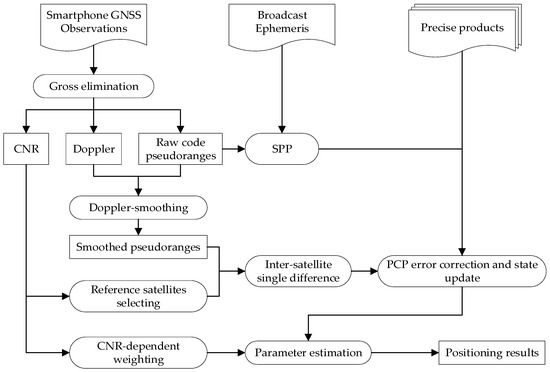
Figure 5.
Flow diagram of PCP processing.
Table 5.
Data processing strategies.
4. Results and Discussion
In this section, the validation of the PCP models introduced in Section 3 was conducted using the dataset mentioned in Section 2. Table 5 presents a comprehensive overview of the processing strategies employed for these PCP models. To ensure statistical significance, the analysis was conducted based on half of the total observation duration. It is important to note that for HP40, only B1I measurements were available for BDS-3. Consequently, the DF-P1I model and TF-P1I models’ positionings were identical, just as they were for IFUC12P1I and IFUC123P1I models.
4.1. Static Test
This section presents the static PCP models for positioning in the static open-sky and complex scenario. Figure 6 shows the HP40 and Mi11 positioning errors in the static open-sky scenario.
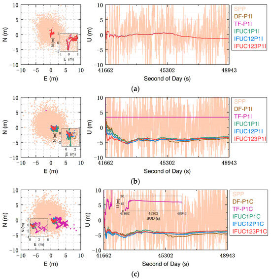
Figure 6.
Position errors in the static open-sky scenario. (a) HP40 positioning errors in IF-P1I and IFUC-P1I models; (b) Mi11 positioning errors in IF-P1I and IFUC-P1I models; (c) Mi11 positioning errors in IF-P1C and IFUC-P1C models.
Figure 6b,c illustrate that for the Mi11 TF-P1I and TF-P1C models, there was a jump in positioning shortly after the start. Upon comparing the results in Table 6, it can be observed that TF-P1I impacts horizontal positioning accuracy, whereas TF-P1C affects U-direction positioning accuracy. This phenomenon may be attributed to a high number of observed BDS-3 triple-frequency data satellites and clock jumps in the second-frequency observation data. It suggests that the quality control method for B2a observations may not be stringent enough. However, the other PCP models, apart from those mentioned above, exhibited consistent positioning performance.
Table 6.
RMSE results and improvement percentages compared to SPP in the static open-sky scenario.
The PCP models’ positioning root mean square error (RMSE) and improvement percentage compared to SPP are presented in Table 6. Figure 7 shows the PCP models’ positioning RMSE in the static scenario. Table 6 and Figure 7a clearly demonstrate that the positioning performance of HP40 exceeded that of Mi11. Additionally, for Mi11, the choice is between B1I or B1C as the ionosphere-corrected pseudo-range did not have a significant impact in the current scenario. For Mi11, there was a slight improvement in U direction positioning accuracy in the IF-P1I and IFUC-P1I models compared to the IF-P1C and IFUC-P1C models. Conversely, the horizontal positioning performance showed a slight improvement in the IF-P1C models and IFUC-P1C models.
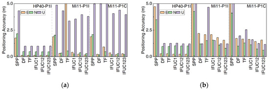
Figure 7.
Positioning accuracy in the static scenario. (a) In the static open-sky scenario; (b) in the static complex scenario.
The PCP models, except for TF-P in Mi11, showed significant improvements over SPP. For HP40, the PCP models achieved sub-meter-level accuracy in the east (E) and north (N) directions, and meter-level accuracy in the upwards (U) direction. These improvements represent increases of approximately 92%, 78%, and 77% in each direction, respectively, compared to SPP. Similarly, for Mi11, the PCP models achieved sub-meter accuracy in the E and N directions, and approximately 4–5-m accuracy in the U direction. Compared to SPP, each direction saw an improvement of about 85%, 87%, and 16%, respectively.
Figure 8 represents the positioning errors of both HP40 and Mi11 in the static complex scenario. The RMSE and improvement percentages of the PCP models compared to SPP are detailed in Table 7. As shown in Figure 8, a decrease in positioning accuracy can be observed for HP40 in the horizontal plane of Mi11 in the static complex scenario due to partial obscuration of satellite observations. For Mi11, a similar jump phenomenon occurred in both the static open-sky and complex scenarios, but its amplitude was smaller in the latter case. The decrease in amplitude may have resulted from obstacles hindering weak satellite signals in the complex scenario. Apart from this phenomenon, the other PCP models exhibited similar performance in terms of positioning accuracy.
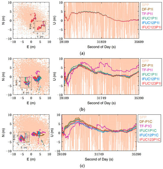
Figure 8.
Position errors in the static complex scenario. (a) HP40 positioning errors in the IF-P1I and IFUC-P1I models; (b) Mi11 positioning errors in the IF-P1I and IFUC-P1I models; (c) Mi11 positioning errors in the IF-P1C and IFUC-P1C models.
Table 7.
RMSE results and improvement percentages compared to SPP in the static complex scenario.
Table 7 and Figure 7b show that HP40 exhibited better positioning performance in both HP40 and Mi11. Additionally, for Mi11, the positioning performance was slightly better in the IF-P1C and IFUC-P1C models than in the IF-P1I and IFUC-P1I models.
The PCP models demonstrated significant improvements over SPP. For HP40, the PCP models achieved sub-meter-level accuracy in the E direction and meter-level accuracy in the N and U directions. These improvements represent an increase of approximately 94%, 71%, and 88% in each direction, respectively, compared to SPP. Similarly, for Mi11, the PCP models achieved approximately two meters of accuracy in the E direction and meter-level accuracy in the N and U directions, except for the TF-P model. Compared to SPP, there was an improvement of about 68%, 75%, and 90% in each direction, respectively.
In the static test, it could be observed that increasing the number of frequencies can improve positioning accuracy. The IFUC12 and IFUC123 models exhibited similar positioning performance, indicating that they may have reached the accuracy limit of the PCP models.
When comparing different static scenarios, the TF-P model in Mi11 was found to perform the worst among the PCP models. This could be attributed to the quality control method for the TF-P model observations not being rigorous. Additionally, in the complex scenario, the U-direction positioning performance was better than in the open-sky scenario. This improvement could be due to the complex environment blocking some satellite signals with weak anti-interference capabilities. Furthermore, HP40 outperformed Mi11 primarily because of its superior satellite tracking abilities.
4.2. Dynamic Test
In dynamic experiments, the determination of the direction between the smartphones and the receiver is not possible without the use of additional sensors. However, a preset value for the horizontal deviation distance between them is in place. Therefore, in dynamic experiments, the deviations in the horizontal plane and U-direction RMSE were calculated.
Figure 9 shows the positioning errors of HP40 and Mi11 in the dynamic scenes. The left side of each picture is a typical urban scenario, and the right side is a complex urban scenario. From Figure 9, it can be observed that the positioning results were discontinuous due to the low-cost receiver. In some places, it observed too few satellite data to provide a reference position. For this, the CHC i70 and smartphones’ positioning rate was calculated, which is the ratio of the number of solution position epochs to the number of observation epochs. The results show that for HP40, the positioning rate in all dynamic scenarios was 100%, while for Mi11, the positioning rate in the dynamic typical urban environment was 98.94%, and it was approximately 98.8% in the dynamic complex urban environment. For CHC i70, the position rate in the dynamic typical urban environment was 86.63%, while it dropped to as low as 46.02% in the dynamic complex urban environment.
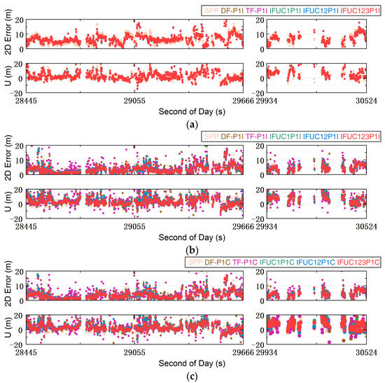
Figure 9.
Position errors in the dynamic scenario. (a) HP40 positioning errors in the IF-P1I and IFUC-P1I models; (b) Mi11 positioning errors in the IF-P1I and IFUC-P1I models; (c) Mi11 positioning errors in the IF-P1C and IFUC-P1C models.
Conclusions about the positioning performance of each PCP model cannot be directly drawn from Figure 9. Table 8 and Table 9 show the positioning RMSE in the dynamic typical and complex urban scenarios, respectively. Figure 10 shows the PCP models’ positioning accuracy.
Table 8.
RMSE results and improvement percentages compared to SPP in the dynamic typical urban scenario.
Table 9.
RMSE results and improvement percentages compared to SPP in the dynamic complex urban scenario.
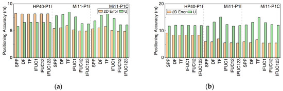
Figure 10.
Positioning accuracy of dynamic scenarios. (a) In the typical urban scenario; (b) in the complex urban scenario.
From Table 8 and Table 9 and Figure 10, it can be observed that the positioning performance of the PCP models was not significantly improved. Compared to SPP, some PCP models showed only a modest improvement, with an increase of around 10% in positioning accuracy in the horizontal plane or U direction. Otherwise, the TF-P model, compared to other PCP models for Mi11, also had the worst positioning performance in both the typical and complex dynamic urban scenarios. This is the same as static test. It could be inferred that the TF-P model is not fully suitable for Mi11 under the same quality control method.
Combined with Section 2, it could be observed that during the dynamic test, the overall satellite tracking ability of the smartphone is affected by the environment and frequent lock loss occurs. In addition, since low-cost receivers cannot continuously provide reference positions, while the positioning rate of smartphones reaches more than 98%, this will cause the smartphone to re-converge when the receiver provides a new reference position. All of this will affect the obtained position accuracy.
5. Conclusions
This study focused on ionosphere-free precise code positioning based on BDS-3/GPS/Galileo multi-frequency pseudo-range observation data obtained with smartphones. Precise code positioning models were proposed, using Doppler smoothing pseudo-range and inter-satellite single difference methods, and the reference satellite was selected using the CNR-weighting method. As for ionospheric delay, precise ionospheric products were used for correction, or the ionosphere-free combination was applied for elimination. The IF-P model contains not only the traditional ionosphere-free combination, but also the single ionosphere-corrected pseudo-range. The IFUC model is composed of ionosphere-corrected pseudo-ranges.
Real-world collected datasets from Huawei P40 and Xiaomi 11 Lite smartphones were used to validate the PCP models, and the results of a quality investigation were presented. In the static open-sky scenario, it was observed that the CNR of multi-GNSS signals was concentrated in the range of 25-40 dB-Hz. Specifically, for HP40, the CNR of the B2a/L5/E5a signal was approximately 10 dB-Hz lower than that of B1C/B1I/L1/E1, whereas for Mi11, it was approximately 6 dB-Hz lower. In the dynamic urban scenarios, the quality of the smartphones’ GNSS observations was significantly degraded, characterized by low CNR values and frequent loss of satellites tracking. When comparing the static open-sky scenario to the static complex scenario and dynamic scenarios, it was observed that the number of visible satellites for HP40 remained relatively stable but was generally lower than that for Mi11. This indicates that Mi11 exhibits superior satellite observation decoding performance compared to HP40, but it lags behind HP40 in terms of satellite tracking ability.
Finally, static and dynamic positioning tests were carried out. The static tests demonstrated that the PCP models can achieve sub-meter-level accuracy in the E and N directions, while achieving meter-level accuracy in the U direction. Numerically, the root mean square error (RMSE) improvement percentages were approximately 93.8%, 75%, and 82.8% for HP40 in the E, N, and U directions, respectively, in both the open-sky and complex scenarios compared to SPP. In the open-sky scenario, Mi11 showed an average increase of about 85.6%, 87%, and 16% in the E, N, and U directions, respectively, compared to SPP. In the complex scenarios, Mi11 exhibited an average increase of roughly 68%, 75.9%, and 90% in the E, N, and U directions, respectively, compared to SPP. However, in the dynamic scenarios, several factors contributed to a decrease in positioning accuracy. These factors include loose quality-control methods, complex environments, and the receiver’s inability to continuously provide reference positions. As a result, in dynamic scenarios, the positioning accuracy typically ranges from 5 to 8 m in the horizontal plane and is 10 m or more in the U direction. Numerically, the PCP models only provided an improvement of approximately 10% in the horizontal plane or U direction compared to SPP. It is worth noting that the IFUC123 model exhibited the best positioning performance, while the TF-P model performed the worst, likely due to the less rigorous quality control of B2a pseudo-range data. Further research will continue to delve deeper into these challenges.
In summary, the PCP models have demonstrated their capability to significantly enhance the positioning accuracy of smartphones under static scenarios. However, it is acknowledged that dynamic scenarios present unique challenges, and further in-depth research is needed to achieve high-precision positioning for smartphones in dynamic environments.
Author Contributions
Conceptualization, R.W. and C.H.; methodology, R.W.; software, R.W.; validation, R.W., C.H., Z.W., F.Y. and Y.W.; formal analysis, R.W.; investigation, C.H. and Y.W.; resources, C.H. and Z.W.; data curation, C.H. and F.Y.; writing—original draft preparation, R.W.; writing—review and editing, R.W., C.H., Z.W., F.Y. and Y.W.; visualization, R.W.; supervision, C.H. and Z.W.; project administration, C.H. and Z.W.; funding acquisition, C.H. All authors have read and agreed to the published version of the manuscript.
Funding
This research was funded by the National Key Research and Development Program of China (Grant No. 2020YFA0713502), the National Natural Science Foundation of China (Grant No. 41874039), Natural Science Foundation of Jiangsu Province, No. BK20191342, the Natural Science Foundation of Anhui Colleges (Grant No. KJ2020A0310) and Anhui Natural Science Foundation (Grant No. 2108085QD173).
Data Availability Statement
Due to restrictions, data are only available upon request.
Acknowledgments
The authors gratefully acknowledge WUM and GFZ for providing the precise products, and CAS for providing the DCB and GIM products. Ruiguang Wang would like to thank Fang Yuan for her continuous companionship and support.
Conflicts of Interest
Author Yangyang Wang was employed by company Qianxun Spatial Intelligence Inc. The remaining authors declare that the research was conducted in the absence of any commercial or financial relationships that could be construed as a potential conflict of interest.
References
- Yang, S.; Xu, Y.; Xu, T.; Jiang, N. Analysis on the PPP Performance of Android Smart-Phone: A Case Study of Huawei P40 Pro. In Proceedings of the China Satellite Navigation Conference (CSNC 2022) Proceedings, Beijing, China, 22–25 May 2022; Yang, C., Xie, J., Eds.; Springer Nature: Singapore, 2022; pp. 363–373. [Google Scholar]
- Zangenehnejad, F.; Gao, Y. GNSS Smartphones Positioning: Advances, Challenges, Opportunities, and Future Perspectives. Satell. Navig. 2021, 2, 24. [Google Scholar] [CrossRef]
- Liu, W.; Wu, M.; Zhang, X.; Wang, W.; Ke, W.; Zhu, Z. Single-Epoch RTK Performance Assessment of Tightly Combined BDS-2 and Newly Complete BDS-3. Satell. Navig. 2021, 2, 6. [Google Scholar] [CrossRef]
- Odolinski, R.; Teunissen, P.J.G.; Odijk, D. Combined BDS, Galileo, QZSS and GPS Single-Frequency RTK. GPS Solut. 2015, 19, 151–163. [Google Scholar] [CrossRef]
- Banville, S.; Van Diggelen, F. Precise Positioning Using Raw GPS Measurements from Android Smartphones. GPS World 2016, 27, 43–48. [Google Scholar]
- Zhang, K.; Jiao, F.; Li, J. The Assessment of GNSS Measurements from Android Smartphones. In China Satellite Navigation Conference (CSNC) 2018 Proceedings; Sun, J., Yang, C., Guo, S., Eds.; Lecture Notes in Electrical Engineering; Springer: Singapore, 2018; Volume 499, pp. 147–157. ISBN 9789811300288. [Google Scholar]
- Zhang, X.; Tao, X.; Zhu, F.; Shi, X.; Wang, F. Quality Assessment of GNSS Observations from an Android N Smartphone and Positioning Performance Analysis Using Time-Differenced Filtering Approach. GPS Solut. 2018, 22, 70. [Google Scholar] [CrossRef]
- Liu, W.; Shi, X.; Zhu, F.; Tao, X.; Wang, F. Quality Analysis of Multi-GNSS Raw Observations and a Velocity-Aided Positioning Approach Based on Smartphones. Adv. Space Res. 2019, 63, 2358–2377. [Google Scholar] [CrossRef]
- Robustelli, U.; Paziewski, J.; Pugliano, G. Observation Quality Assessment and Performance of GNSS Standalone Positioning with Code Pseudoranges of Dual-Frequency Android Smartphones. Sensors 2021, 21, 2125. [Google Scholar] [CrossRef] [PubMed]
- Banville, S.; Lachapelle, G.; Ghoddousi-Fard, R.; Gratton, P. Automated Processing of Low-Cost GNSS Receiver Data. In Proceedings of the 32nd International Technical Meeting of the Satellite Division of the Institute of Navigation (ION GNSS+ 2019), Miami, FL, USA, 16–20 September 2019; pp. 3636–3652. [Google Scholar]
- Lachapelle, G.; Gratton, P.; Horrelt, J.; Lemieux, E.; Broumandan, A. Evaluation of a Low Cost Hand Held Unit with GNSS Raw Data Capability and Comparison with an Android Smartphone. Sensors 2018, 18, 4185. [Google Scholar] [CrossRef]
- Privat, A.; Pascaud, M.; Laurichesse, D. Innovative Smartphone Applications for Precise Point Positioning. In Proceedings of the 2018 SpaceOps Conference; American Institute of Aeronautics and Astronautics, Marseille, France, 28 May 2018. [Google Scholar]
- Aggrey, J.; Bisnath, S.; Naciri, N.; Shinghal, G.; Yang, S. Multi-GNSS Precise Point Positioning with next-Generation Smartphone Measurements. J. Spat. Sci. 2020, 65, 79–98. [Google Scholar] [CrossRef]
- Gill, M.; Bisnath, S.; Aggrey, J.; Seepersad, G. Precise Point Positioning (PPP) Using Low-Cost and Ultra-Low-Cost GNSS Receivers. In Proceedings of the 30th International Technical Meeting of the Satellite Division of the Institute of Navigation (ION GNSS+ 2017), Portland, OR, USA, 25–29 September 2017; pp. 226–236. [Google Scholar]
- Guo, L.; Wang, F.; Sang, J.; Lin, X.; Gong, X.; Zhang, W. Characteristics Analysis of Raw Multi-GNSS Measurement from Xiaomi Mi 8 and Positioning Performance Improvement with L5/E5 Frequency in an Urban Environment. Remote Sens. 2020, 12, 744. [Google Scholar] [CrossRef]
- Fortunato, M.; Critchley-Marrows, J.; Siutkowska, M.; Ivanovici, M.L.; Benedetti, E.; Roberts, W. Enabling High Accuracy Dynamic Applications in Urban Environments Using PPP and RTK on Android Multi-Frequency and Multi-GNSS Smartphones. In Proceedings of the 2019 European Navigation Conference (ENC), Warsaw, Poland, 9–12 April 2019; IEEE: Piscataway, NJ, USA, 2019; pp. 1–9. [Google Scholar]
- Roberts, W.; Critchley-Marrows, J.; Fortunato, M.; Ivanovici, M.; Callewaert, K.; Tavares, T.; Arzel, L.; Pomies, A. FLAMINGO-Fulfilling Enhanced Location Accuracy in the Mass-Market through Initial Galileo Services. In Proceedings of the 31st International Technical Meeting of the Satellite Division of the Institute of Navigation (ION GNSS+ 2018), Miami, FL, USA, 24–28 September 2018; pp. 489–502. [Google Scholar]
- Robustelli, U.; Baiocchi, V.; Pugliano, G. Assessment of Dual Frequency GNSS Observations from a Xiaomi Mi 8 Android Smartphone and Positioning Performance Analysis. Electronics 2019, 8, 91. [Google Scholar] [CrossRef]
- Elmezayen, A.; El-Rabbany, A. Precise Point Positioning Using World’s First Dual-Frequency GPS/GALILEO Smartphone. Sensors 2019, 19, 2593. [Google Scholar] [CrossRef] [PubMed]
- Wu, Q.; Sun, M.; Zhou, C.; Zhang, P. Precise Point Positioning Using Dual-Frequency GNSS Observations on Smartphone. Sensors 2019, 19, 2189. [Google Scholar] [CrossRef] [PubMed]
- Aggrey, J.; Bisnath, S.; Naciri, N.; Shinghal, G.; Yang, S. Use of PPP Processing for Next-Generation Smartphone GNSS Chips: Key Benefits and Challenges. In Proceedings of the 32nd International Technical Meeting of the Satellite Division of the Institute of Navigation (ION GNSS+ 2019), Miami, FL, USA, 16–20 September 2019; pp. 3862–3878. [Google Scholar]
- Psychas, D.; Bruno, J.; Massarweh, L.; Darugna, F. Towards Sub-Meter Positioning Using Android Raw GNSS Measurements. In Proceedings of the 32nd International Technical Meeting of the Satellite Division of the Institute of Navigation (ION GNSS+ 2019), Miami, FL, USA, 16–20 September 2019; pp. 3917–3931. [Google Scholar]
- Laurichesse, D.; Privat, A. An Open-Source PPP Client Implementation for the CNES PPP-WIZARD Demonstrator. In Proceedings of the 28th International Technical Meeting of the Satellite Division of the Institute of Navigation (ION GNSS+ 2015), Tampa, FL, USA, 14–18 September 2015; pp. 2780–2789. [Google Scholar]
- Geng, J.; Jiang, E.; Li, G.; Xin, S.; Wei, N. An Improved Hatch Filter Algorithm towards Sub-Meter Positioning Using Only Android Raw GNSS Measurements without External Augmentation Corrections. Remote Sens. 2019, 11, 1679. [Google Scholar] [CrossRef]
- Li, G.; Long, C.; Wang, F. Synchronizing and Integrating Android Multi-GNSS/Accelerometer Sensors to Capture Broadband Vibrations at Sub-Centimeter Resolution. In Proceedings of the 33rd International Technical Meeting of the Satellite Division of the Institute of Navigation (ION GNSS+ 2020), Online, 22–25 September 2020; pp. 3612–3625. [Google Scholar]
- Paziewski, J.; Sieradzki, R.; Baryla, R. Signal Characterization and Assessment of Code GNSS Positioning with Low-Power Consumption Smartphones. GPS Solut. 2019, 23, 98. [Google Scholar] [CrossRef]
- Zeng, S.; Kuang, C.; Yu, W. Evaluation of Real-Time Kinematic Positioning and Deformation Monitoring Using Xiaomi Mi 8 Smartphone. Appl. Sci. 2022, 12, 435. [Google Scholar] [CrossRef]
- Shang, R.; Gao, C.; Gan, L.; Zhang, R.; Gao, W.; Meng, X. Multi-GNSS Differential Inter-System Bias Estimation for Smartphone RTK Positioning: Feasibility Analysis and Performance. Remote Sens. 2023, 15, 1476. [Google Scholar] [CrossRef]
- Wang, L.; Li, Z.; Zhao, J.; Zhou, K.; Wang, Z.; Yuan, H. Smart Device-Supported BDS/GNSS Real-Time Kinematic Positioning for Sub-Meter-Level Accuracy in Urban Location-Based Services. Sensors 2016, 16, 2201. [Google Scholar] [CrossRef]
- Zhang, K.; Jiao, W.; Wang, L.; Li, Z.; Li, J.; Zhou, K. Smart-RTK: Multi-GNSS Kinematic Positioning Approach on Android Smart Devices with Doppler-Smoothed-Code Filter and Constant Acceleration Model. Adv. Space Res. 2019, 64, 1662–1674. [Google Scholar] [CrossRef]
- Geng, J.; Long, C.; Li, G. A Robust Android Gnss Rtk Positioning Scheme Using Factor Graph Optimization. IEEE Sens. J. 2023, 23, 13280–13291. [Google Scholar] [CrossRef]
- Jiang, Y.; Gao, Y.; Ding, W.; Liu, F.; Gao, Y. An Improved Ambiguity Resolution Algorithm for Smartphone RTK Positioning. Sensors 2023, 23, 5292. [Google Scholar] [CrossRef] [PubMed]
- Tao, X.; Liu, W.; Wang, Y.; Li, L.; Zhu, F.; Zhang, X. Smartphone RTK Positioning with Multi-Frequency and Multi-Constellation Raw Observations: GPS L1/L5, Galileo E1/E5a, BDS B1I/B1C/B2a. J. Geod. 2023, 97, 43. [Google Scholar] [CrossRef]
- GSA. Using GNSS Raw Measurements on Android Devices; The GSA GNSS Raw Measurements Task Force: Prague, Czech Republic, 2017. [Google Scholar]
- Li, G.; Geng, J. Characteristics of Raw Multi-GNSS Measurement Error from Google Android Smart Devices. GPS Solut. 2019, 23, 90. [Google Scholar] [CrossRef]
- Wu, Z.; Liu, P.; Liu, Q.; Wang, Y. MEMS-Based IMU Assisted Real Time Difference Using Raw Measurements from Smartphone. In Proceedings of the 31st International Technical Meeting of the Satellite Division of the Institute of Navigation (ION GNSS+ 2018), Miami, FL, USA, 24–28 September 2018; pp. 445–454. [Google Scholar]
- Li, G. Theory and Method of GNSS Ambiguity Resolution for Smartphones; Wuhan University: Wuhan, China, 2021. [Google Scholar]
- Wu, Z.; Wang, Q.; Hu, C.; Yu, Z.; Wu, W. Modeling and Assessment of Five-Frequency BDS Precise Point Positioning. Satell. Navig. 2022, 3, 8. [Google Scholar] [CrossRef]
- Hu, C.; Wang, Q.; Wu, Z.; Guo, Z. A Mixed Multi-Frequency Precise Point Positioning Strategy Based on the Combination of BDS-3 and GNSS Multi-Frequency Observations. Meas. Sci. Technol. 2023, 34, 025008. [Google Scholar] [CrossRef]
- Saastamoinen, J. Atmospheric Correction for the Troposphere and Stratosphere in Radio Ranging Satellites. In The Use of Artificial Satellites for Geodesy; American Geophysical Union (AGU): Washington, DC, USA, 1972; pp. 247–251. ISBN 978-1-118-66364-6. [Google Scholar]
- Nie, Z.; Liu, F.; Gao, Y. Real-Time Precise Point Positioning with a Low-Cost Dual-Frequency GNSS Device. GPS Solut. 2020, 24, 9. [Google Scholar] [CrossRef]
- Montenbruck, O.; Steigenberger, P.; Hauschild, A. Broadcast versus Precise Ephemerides: A Multi-GNSS Perspective. GPS Solut. 2015, 19, 321–333. [Google Scholar] [CrossRef]
- Chen, L.; Li, M.; Zhao, Y.; Hu, Z.; Zheng, F.; Shi, C. Multi-GNSS Real-Time Precise Clock Estimation Considering the Correction of Inter-Satellite Code Biases. GPS Solut. 2021, 25, 32. [Google Scholar] [CrossRef]
- Pan, L.; Zhang, X.; Guo, F.; Liu, J. GPS Inter-Frequency Clock Bias Estimation for Both Uncombined and Ionospheric-Free Combined Triple-Frequency Precise Point Positioning. J. Geod. 2019, 93, 473–487. [Google Scholar] [CrossRef]
- Wang, Z.; Wang, R.; Wang, Y.; Hu, C.; Liu, B. Modelling and Assessment of a New Triple-Frequency IF1213 PPP with BDS/GPS. Remote Sens. 2022, 14, 4509. [Google Scholar] [CrossRef]
- Wanninger, L.; Heßelbarth, A. GNSS Code and Carrier Phase Observations of a Huawei P30 Smartphone: Quality Assessment and Centimeter-Accurate Positioning. GPS Solut. 2020, 24, 64. [Google Scholar] [CrossRef]
- Zhou, Z.; Li, B. Optimal Doppler-Aided Smoothing Strategy for GNSS Navigation. GPS Solut. 2017, 21, 197–210. [Google Scholar] [CrossRef]
- Wang, L.; Li, Z.; Wang, N.; Wang, Z. Real-Time GNSS Precise Point Positioning for Low-Cost Smart Devices. GPS Solut. 2021, 25, 69. [Google Scholar] [CrossRef]
- Schmid, R.; Steigenberger, P.; Gendt, G.; Ge, M.; Rothacher, M. Generation of a Consistent Absolute Phase-Center Correction Model for GPS Receiver and Satellite Antennas. J. Geod. 2007, 81, 781–798. [Google Scholar] [CrossRef]
Disclaimer/Publisher’s Note: The statements, opinions and data contained in all publications are solely those of the individual author(s) and contributor(s) and not of MDPI and/or the editor(s). MDPI and/or the editor(s) disclaim responsibility for any injury to people or property resulting from any ideas, methods, instructions or products referred to in the content. |
© 2023 by the authors. Licensee MDPI, Basel, Switzerland. This article is an open access article distributed under the terms and conditions of the Creative Commons Attribution (CC BY) license (https://creativecommons.org/licenses/by/4.0/).