Article

The Impact and Correction of Sensitive Environmental Factors on Spectral Reflectance Measured In Situ

1
Key Laboratory of Precision Opto-Mechatronics Technology, Ministry of Education, School of Instrumentation and Optoelectronic Engineering, Beihang University, Beijing 100191, China
2
Key Laboratory of Ministry of Industry and Information Technology, Institute of Artificial Intelligence, Aerospace Optical-Microwave Integrated Precision Intelligent Sensing, Beihang University, Beijing 100191, China
3
Land Satellite Remote Sensing Application Center, Ministry of Natural Resources of China, Beijing 100048, China
4
Science & Technology on Integrated Information System Laboratory, Institute of Software, Chinese Academy of Sciences, Beijing 100190, China
*
Author to whom correspondence should be addressed.
These authors contributed equally to this work.
Remote Sens. 2023, 15(22), 5332; https://doi.org/10.3390/rs15225332
Submission received: 23 September 2023 / Revised: 8 November 2023 / Accepted: 10 November 2023 / Published: 12 November 2023
(This article belongs to the Special Issue In Situ Data in the Interplay of Remote Sensing II)

Abstract

:
The spectral reflectance measured in situ is often regarded as the “truth” of objects, which plays an important role in Earth observation applications. However, in situ measurements are influenced by several factors such as atmospheric conditions, illumination and view geometry (I&VG), cloud coverage, and adjacency effects. In order to avoid the influence of these factors, in situ measurements are usually carried out under sunny days and close to noon. However, the impact of I&VG is still present in most cases. At present, people still know little about the influence mechanism of I&VG. Moreover, correcting the impact of I&VG is also a problem that needs to be urgently solved in reflectance spectroscopy. In this work, experiments are carried out using the multi-directional hyperspectral remote sensing simulation facility (MHSRS2F), which allows adjustment and control of the I&VG parameters. This paper proposes an uncertainty evaluation model for I&VG and quantifies the uncertainty caused by different I&VG parameters. Then, the sensitivity of reflectance to I&VG at different wavelengths is explored based on uncertainty models. Finally, a correction model for reflectance under different I&VG conditions is proposed. The results reveal that the uncertainty and sensitivity caused by observation height are relatively high, regardless of the surface heterogeneity. It directly affects the size of the field of view and the physicochemical characteristics of the object. For objects that approximate the Lambertian surface, more attention should be paid to the selection and variation of solar and view zenith angles and view azimuth angles. For objects with surface heterogeneity, the selection and variation of solar azimuth angle, view azimuth angle, and solar zenith angle are more crucial. The correction model proposed in this paper has a 41.25% correction effect on different view zenith angles, but the correction effect on other environmental factors is not significant.

1. Introduction

Field spectroscopy has become an important technology for characterizing the reflectance features of natural surfaces and has received increasing attention in the last two decades [1]. The advantage of field spectroscopy is that the portable spectrometers can remain fixed over the object for a longer time, and the shorter path length between the instrument and object reduces the influence of the atmosphere [2]. Therefore, in situ measurements are often used as the truth of objects and plays an important role in the applications of Earth observation and environmental monitoring systems [3]. The main applications include the following: the vicarious calibration of remote sensors [4]; the correction of atmospheric effects on airborne or spaceborne images [5]; the validation of the quantitative remote sensing data products [6]; the identification and classification of the targets from images [7]; the establishment of models of biophysical attributes, biological processes, and remote sensing feature attributes [8]; the prediction of the best spectral bands, geometric configurations, and the optimum time for a specific task [9]; and the supplementation of the spectral library.
In situ measurements are easily influenced by environmental factors, such as atmospheric conditions, illumination intensity, illumination and view geometry (I&VG), sky cloud coverage, and the adjacency effects, which lead to the phenomenon that the same objects have different spectra [10]. In order to avoid the influence of environmental factors, in situ measurements are usually made under sunny days and close to noon. However, the influence of I&VG is still present in most cases. In fact, the prerequisite for achieving ideal results in various applications based on in situ measurement is synchronous observation on the ground and airborne or spaceborne observation. This means that in situ measurements need to ensure that environmental conditions are consistent with the airborne or spaceborne data, especially the angle conditions, field of view, etc. [11,12]. However, practice has proven that synchronous observation is difficult to realize. At the same time, it is difficult to maintain the same observation height for in situ measurements. Due to the heterogeneity of most land surfaces, the change in field of view caused by different observation heights inevitably leads to fluctuations in spectral reflectance [13]. Moreover, many models are based on the Lambertian surface hypothesis [14]. However, most natural features are non-Lambertian, and the changes in spectral reflectance measured in situ caused by illumination conditions, viewing geometry, and field of view will inevitably affect the validation accuracy of a model based on the Lambertian hypothesis. Therefore, this article mainly discusses the influence of I&VG on in situ measurements of objects with different degrees of surface heterogeneity.
At present, the uncertainty of spectral reflectance measured in situ caused by I&VG has been widely studied. There are two common approaches to studying this uncertainty: in the laboratory and in the natural environment. Instruments such as LAGOS, CLabSpeG, and FIGIGO are designed to obtain the bidirectional reflection factor (BRF) of different objects in the laboratory [15,16,17]. Meanwhile, a lot of research on the influence of I&VG is conducted outdoors. The BRF varies with solar position, viewing plane and angles, and sensor FOV and distance combinations [18]. The measurement uncertainty value of spectral reflectance caused by solar radiation can reach 5% to 10% [10]. Gu et al. revealed that around solar noon, the solar zenith angle only changes slightly within 0.2%. When the view zenith angle changes from 0° to 30°, the variation in BRDF can reach 10% [19]. Anderson et al. investigated the effect of solar zenith angle on reflectance ranges from 16% to 32% [20].
Despite these advances, many problems have not yet been fully investigated. A challenging problem in uncertainty evaluation based on laboratories is that it is difficult to simulate real field environmental conditions. The main problem of research based on in situ measurements is that I&VG are uncontrollable. This has created an issue where the uncertainty results of measurement data are inconsistent under different I&VG conditions. In addition, it is unfeasible to collect spectral reflectance under all I&VG conditions. This results in the fact that the comprehensive quantitative evaluation of uncertainty results caused by I&VG is rarely performed. Therefore, current applications based on in situ measurements still use a single spectrum as the reference truth, which limits the reliability of subsequent application results [3].
Another problem with these two research methods is that the uncertainty caused by I&VG is formed by the coupling of multiple I&VG parameters. Because the decoupling of multiple I&VG parameters is still a significant challenge, the effect mechanism of any single I&VG parameter is still poorly understood [21]. Based on the understanding of the influence of I&VG, correcting the influence of different I&VG conditions on spectral reflectance and normalizing different I&VG conditions are other problems that need to be urgently solved.
To address the above limitations, this study takes rocks as the target object, which can maintain their physicochemical properties for a long time. In this work, five I&VG parameters, namely, solar and view azimuth angles, solar and view zenith angles, and observation height, were experimented using the MHSRS2F [22]. The MHSRS2F can simulate the outdoor environment more realistically and allows adjustment and control of the I&VG parameters. Based on the experimental results, an uncertainty evaluation model for I&VG was constructed. In this work, the uncertainty caused by different I&VG parameters was quantified. Then, the sensitivity of spectral reflectance to I&VG at different wavelengths was explored based on the uncertainty models. On the basis of understanding the influence of I&VG, a correction model for reflectance under different I&VG conditions is proposed.

2. Materials and Experimental Design

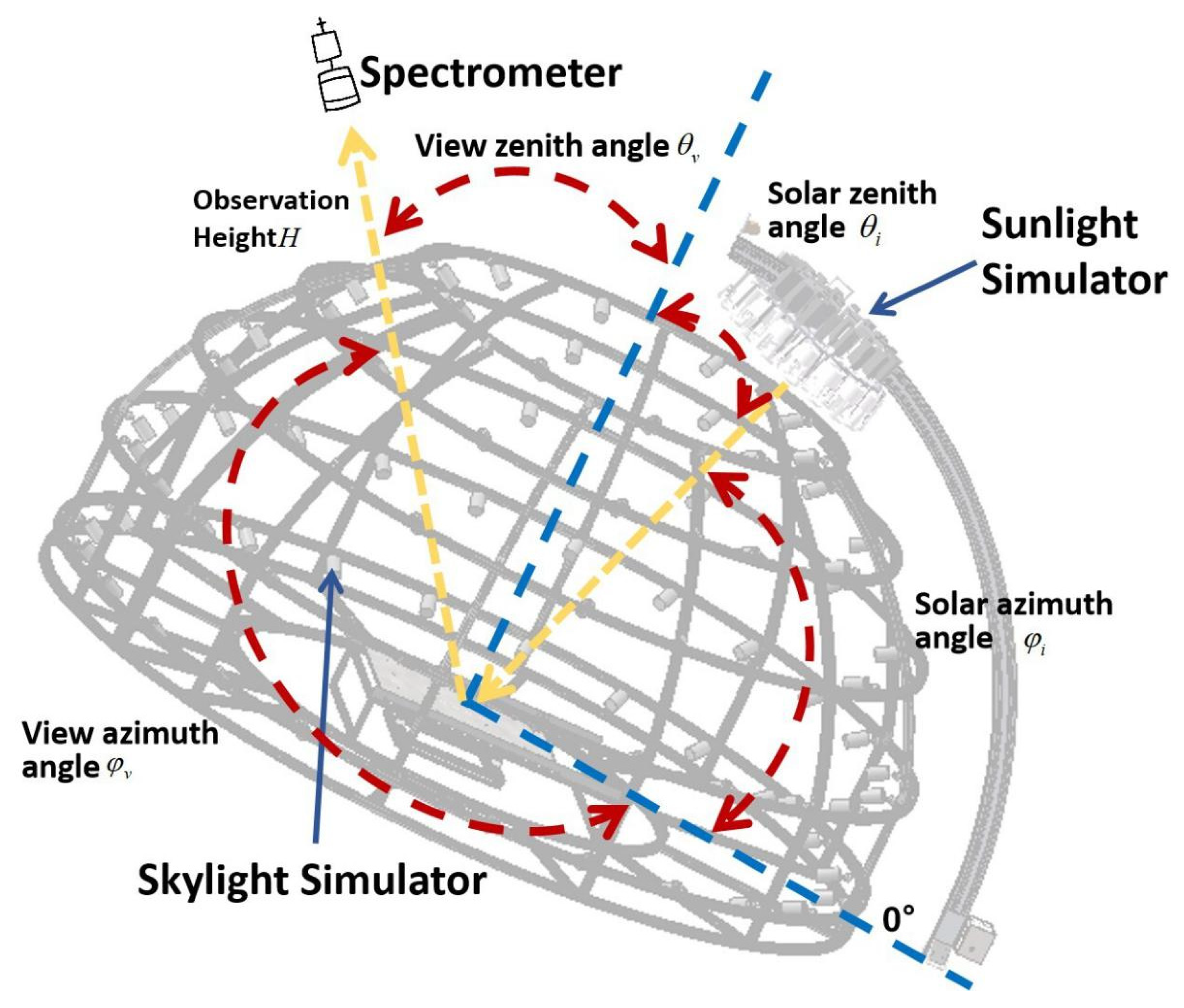
2.1. Experimental Setup

The experimental instruments included the Multi-Directional Hyperspectral Remote Sensing Simulation Facility (MHSRS2F) and the Analytical Spectroscopy DeviceFieldSpec Pro (ASD) spectroradiometer. The MHSRS2F (Figure 1) consists of three parts: a solar simulator, a skylight simulator, and a multi-angle observation simulator [22]. This is specifically designed to obtain the same value as the reflectance factor (RF) acquired in situ by simulating the illumination conditions of sunlight and skylight. After statistical analysis, the spectral correlation coefficients of the simulated solar spectrum and skylight spectrum with the standard spectrum can reach 0.928 and 0.912, respectively. Appendix A and Appendix B provide field environmental simulation experiments and instrument stability tests based on the MHSRS2F. The above experiments prove that the MHSRS2F can stably and accurately simulate the field environmental conditions in the laboratory to collect the hemispherical conical reflectance factor (HCRF).
In addition, the solar and view azimuth angles can be adjusted from 0° to 360°. Solar zenith angles range from 15° to 60°, while view zenith angles span from 0° to 90°. All the spectral reflectance data described in this paper were obtained by using the ASD spectroradiometer with a 5° fore optic lens, which covers the 350–2500 nm spectral range. In this experiment, the SpectralonTM White Diffuse Reflectance Standard (99%) was used as a reference panel to acquire the RF.

2.2. Samples, Sampling Sites, and In Situ Measurements

Ten rock samples collected from the Gobi Desert Mining Area in Hami, Western China, were selected for the experiment (Figure 2). As shown in Figure 3, the collected rock samples encompassed a variety of types, including common sulfides, halides, oxides, carbonates, and silicates. These samples exhibited diverse properties such as different colors, roughness, crystal structures, grain sizes, and gloss levels. The surface area of rock samples was sufficient to fill the field of view of the instrument. Since this research focuses on the impact of environmental conditions, the original-state rocks were used in this experiment.
The spectral reflectance of corresponding rocks was measured at the place where the rock samples were collected, and then the environmental conditions were recorded (Table 1). At the position of each rock sample, 7 measurements were made on the panel and the rock surface, and the measurement sequence was panel, 5 times rock surface, and panel. Each individual measurement consisted of 5 ASD scans. Therefore, a total of 35 in situ measured spectral reflectance were generated for each rock sample.

2.3. Simulation Experiments of Field Environmental Factors

The main purpose of this experiment is to explore the influence of I&VG within the environmental factors on measured reflectance spectra. For near-surface observations, the rock surface is a three-dimensional rather than a smooth plane, and the bidirectional reflection characteristics of rocks formed by different observation and illumination azimuth angles are different. Therefore, this experiment selected the use of absolute azimuth angles instead of relative azimuth angles. In addition, in the process of in situ measurements, the variation in the instrument field of view is usually caused by differences in observation heights. Therefore, this experiment selected five parameters of I&VG, namely solar zenith angle, solar azimuth angle, view zenith angle, view azimuth angle, and observation height, as the research objects.
Based on the latitude of the Mining Area, the annual variation range of solar zenith angle in this region is around 19.2–90°. And the in situ measurement is usually carried out at noon. Therefore, the variation range of solar zenith angle is from 20° to 60°. During in situ measurement, different operators may use different measurement methods, which may lead to differences in observation height. When an adult stands and holds the spectroradiometer probe, the distance between the probe and the target object is usually around 100 cm. Simultaneously, when the observation height is less than 10 cm, it is easy for the shadow caused by the probe to appear on the surface of the measured object. Therefore, the variation range considered in this simulation experiment of observation height ranges from 10 cm to 100 cm. The HCRF of rock samples with different environments is collected by adjusting the sunlight simulator, the skylight simulator, and the multi-angle observation simulator in the MHSRS2F. The specific experimental protocol is shown in Table 2 and Figure 4.

2.4. Surface Heterogeneity Experiment

In order to explore the influence of different I&VG parameters on the measured reflectance spectra with different degrees of surface heterogeneity, the goal of this experiment is to quantify the surface heterogeneity in 10 rock samples. Under the same I&VG conditions, 45 different observation positions of rock samples were selected along the X and Y axes at 2 cm intervals, by using an electronic control translation stage. Since the observation height of the instrument in this experiment is 100 cm and the fore optic lens is 5°, the surface area of the rock sample evaluated in this experiment is around 20 cm × 12 cm (Figure 5). The experimental results show that the root-mean-square error (RMSE) caused by the heterogeneity of 10 rock surfaces is around 0.42–1.62%.

3. Methodology

3.1. Field Data Uncertainty Propagation

For this research based on the MHSRS2F, the simulated in situ measurement values can be decomposed into four independent parts: the part related to geometric variables, the part related to sample surface heterogeneity, the part related to ASD spectroradiometer, and the part related to radiation intensity. Therefore, the simulated in situ measurement model can be expressed as the sum of four independent functions by using an additive model:
f ( x ) = f ( H , θ i , φ i , θ v , φ v ) + f heterogeneity + f ASD + f illumination
where f ( H , θ i , φ i , θ v , φ v ) is a function related to five geometric parameters of I&VG within environmental factors; H refers to the observation height; θ i and θ v are the solar and view zenith angles, respectively; φ i and φ v are the solar and view azimuth angles, respectively; f heterogeneity is a function related to the surface heterogeneity of samples; f ASD is a function related to the ASD spectroradiometer noise; and f illumination is related to the stability of solar radiation intensity and scattered radiation intensity simulated by the MHSRS2F.
According to the measurement model (Equation (1)), a complete evaluation model of spectral uncertainty for in situ measurements caused by I&VG under the MHSRS2F is proposed. Since the measurement model is an implicit model, quantifying the sensitivity coefficient is difficult. Therefore, this section assumes that the uncertainty of each term has a consistent influence on the sensitivity of the measurement uncertainty, and the sensitivity coefficient of each term is ignored in the uncertainty calculation. The total uncertainty caused by I&VG σ total can be given by the following expression:
σ total = ( σ geometry ) 2 + ( σ heterogeneity ) 2 + ( σ ASD ) 2 + ( σ illumination ) 2
where σ total refers to the mean of the standard deviation (SD) of the reflectance spectra collected under different I&VG parameters that is simulated by the MHSRS2F; σ geometry and σ heterogeneity are uncertainties caused by the I&VG and surface heterogeneity of the object, respectively; and σ ASD and σ illumination are uncertainties caused by the ASD spectroradiometer noise and the stability of solar radiation intensity and scattered radiation intensity simulated by the MHSRS2F, respectively.
Therefore, the uncertainty of the objects caused by a single I&VG parameter σ geometry can be expressed as
σ geometry = σ total 2 σ heterogeneity 2 σ A S D 2 σ illumination 2
The uncertainty of each band for the reference panel caused by five parameters of I&VG is calculated based on Formula (3) (Figure 6). Since these five parameters are all geometric variables, their changes in different bands are consistent. In addition, according to the stability experiment in Appendix B, the SD caused by the stability of solar radiation intensity, scattered radiation intensity, and instruments during the long-term experiment ranges from 0.028% to 0.059%. If their influence is ignored, the uncertainty of each band caused by any parameter of I&VG should be the same. However, Figure 6 shows that the uncertainty greatly fluctuates in the range of 350 nm–400 nm, NIR and SWIR regions. This is because the noise of the two sensors in the SWIR of the ASD spectroradiometer is greater than that of the sensors in the VNIR, and using the average noise of all bands as σ ASD , the uncertainty caused by noise in SWIR regions has not been eliminated [23]. The difference between the average uncertainty of the reference panel in all wavebands and in the range of 400–900 nm can be used to represent the portion of the uncertainty caused by the noise of the ASD spectroradiometer in the SWIR region σ ASD _ SWIR that exceeds the average noise value of all bands σ ASD .
Therefore, this paper uses the average uncertainty of the reference panel in the 400–900 nm range to characterize the uncertainty caused by I&VG, which can be considered as noise having no additional impact in the SWIR range. Since the reference panel is considered as a homogeneous surface, the uncertainty of the reference panel caused by a single I&VG σ geometry _ panel can be written as
σ geometry _ panel = σ total 2 σ ASD 2 σ illumination 2
where σ total refers to the mean of the SD of the reference panel in the range of 400–900 nm, and σ ASD refers to the uncertainty caused by the ASD spectroradiometer noise in all bands.
The uncertainty of the rock samples caused by a single I&VG σ geometry _ sample can be written as
σ geometry _ sample = σ total 2 σ heterogeneity 2 σ ASD 2 σ illumination 2 σ ASD _ SWIR 2
where σ total refers to the mean of the SD of the reference panel in all bands, and σ ASD _ SWIR refers to the portion of the uncertainty caused by ASD spectroradiometer noise in the SWIR region that exceeds the average noise value of all bands σ ASD .
For uncertainty caused by the coupling of multiple I&VG parameters, σ geometry is given by the following expression, which is equal to σ geometry in Equation (2):
σ geometry = k × i = 1 n σ i 2 + 2 i = 1 n j = i + 1 n σ i σ j r ( x i , x j )
where n is the number of I&VG parameters; σ i refers to the uncertainty caused by the I&VG parameters i ; x i refers to the average value of repeated measurements under I&VG condition i ; r ( x i , x j ) is the correlation coefficient between two I&VG parameters; and k is the coverage factor, which is taken as 2 in this work.

3.2. Sobol’s Global Sensitivity Analysis

Since the in situ measurement model is an implicit function, it is difficult to quantify the sensitivity coefficient. Therefore, the uncertainty calculation in Section 3.1 ignores the sensitivity coefficients of each term. The innovation of this paper is the use of the spectral reflectance collected by the MHSRS2F to replace the results of the in situ measurement model. According to the variation range of the five I&VG parameters in Table 2, the combination of five I&VG parameters is randomly selected using the random sampling method. The combination of five I&VG parameters obtained through random sampling is set in the MHSRS2F, and then the HCRF of the measured object is collected. A total of 96 experiments were conducted in this work, and a total of 96 sets of experimental data were obtained for subsequent sensitivity analysis.
Sensitivity analysis (SA) of the model output can be used to determine how the model (numerical value or otherwise) depends on its input factors. I.M. proposed Sobol’s Global Sensitivity Analysis method [24]. Global Sensitivity Analysis can not only consider the influence of multiple parameter changes on the output of the model at the same time, but also quantify the influence of the interaction between parameters on the output of the model [25]. The advantage of this method is that the calculation form is simple and there is no requirement for the monotonicity, linearity, and distribution characteristics of the model. Sobol’s method is to decompose the total variance of the output result of the model into the first-order variance of the independent parameters and the higher-order variance of the parameter combination. Then, the ratio of the first-order variance and the higher-order variance to the total variance is calculated to determine the influence of the parameters or parameter interaction on the output of the model. Therefore, the first-order sensitivity index for parameter x i and the total sensitivity index for parameter x i can be defined as
S x i = V x i V ( y ) = V ( E ( y | x i ) ) V ( y )
S T x i = 1 V ~ x i V ( y ) = 1 V ( E ( y | x ~ i ) ) V ( y )
where S x i refers to the first-order sensitivity coefficient, which measures the main effects of x i on the output result f ( x ) ; S T x i refers to the total sensitivity coefficient, which measures the main effects of x i and the effects of the interaction between x i and other parameters; and V ~ x i is the sum of the variance caused by all parameters except x i .

3.3. Field Data Correction Model

Since reflectance cannot be directly measured, the infinitesimal elements of the solid angle do not include measurable amounts of radiant flux [26]. Therefore, the reflectance factor (RF) is proposed as the equivalent coefficient used in practice. It is the ratio of the radiant flux reflected by a surface to that reflected by an ideal diffuse Lambertian standard surface, irradiated under the same illumination and observation conditions [27]. Since a perfectly reflecting panel does not exist in practice, the spectral reflectance of the reference panel needs to be corrected [14]:
R T ( H , θ i , φ i , θ v , φ v ) = L T ( H , θ i , φ i , θ v , φ v ) L P ( H , θ i , φ i , θ v , φ v ) × K
where R T ( H , θ i , φ i , θ v , φ v ) is the RF of the object; L T ( H , θ i , φ i , θ v , φ v ) and L P ( H , θ i , φ i , θ v , φ v ) refer to the radiance of the target objects and reference panel under the same illumination and observation conditions, respectively; and K refers to the panel correction factor.
With the change in I&VG, the radiance of the object and the reference panel will also change at the same time. Because the variation in object radiance with I&VG is related to its physicochemical properties, it is difficult to find the universal law of variation of object radiance with I&VG. However, because the reference panel used in spectrum collection is unchanged, the law of variation of the reference panel radiance with the I&VG can be determined through multiple measurements based on the MHSRS2F.
Therefore, a correction model of spectral reflectance under different I&VG parameters is proposed in this paper. The core concept is to correct the influence of different I&VG parameters on the reference panel, to eliminate the partial of influence of I&VG on the spectral reflectance of the object:
R T _ b e f o r e = L T _ b e f o r e L P _ b e f o r e × K ( L T _ b e f o r e L P _ b e f o r e × L P _ b e f o r e L P _ a f t e r ) × K ( L T _ b e f o r e L P _ a f t e r ) × K R T _ a f t e r
R T _ a f t e r R T _ b e f o r e × L P _ b e f o r e L P _ a f t e r R T _ b e f o r e × C
where R T _ b e f o r e is the RF of the target object under a certain I&VG condition before correction; R T _ a f t e r represents the RF of the target object after correction to the desired I&VG conditions; L T _ b e f o r e and L P _ b e f o r e refer to the radiance of the target object and panel before correction, respectively; and L P _ a f t e r is the panel radiance under desired I&VG conditions.
Therefore, the part L P _ b e f o r e L P _ a f t e r can be defined as a correction factor ( C ) related to the I&VG conditions.
As for the correction work of this article, firstly, the spectral reflectance of two groups of rock samples under different I&VG conditions were collected in the field as experimental data before and after correction, and the corresponding I&VG conditions were recorded. Then, the same I&VG conditions were set in the MHSRS2F and the radiance of the reference panel was collected. And based on the method of locally weighted regression, a correction factor ( C ) under the corresponding I&VG conditions is obtained. Finally, multiplying the RF of the object before correction by the corresponding correction factor ( C ), the RF after correction can be obtained. RMSE is used as an indicator to evaluate correction ability in this work.

4. Results and Discussion

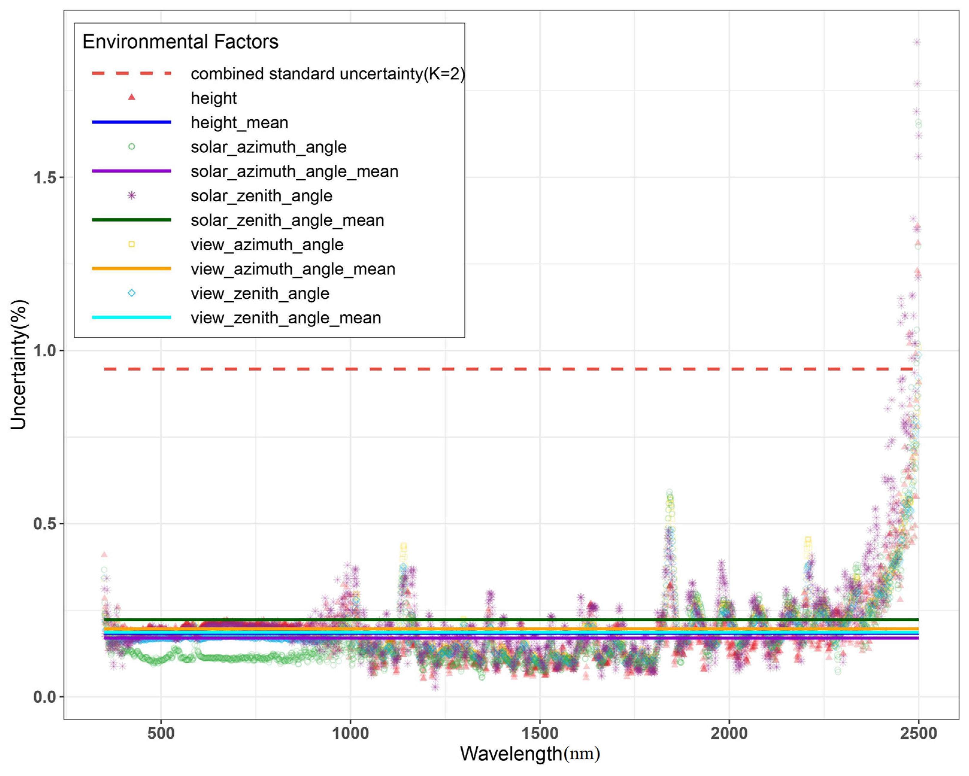
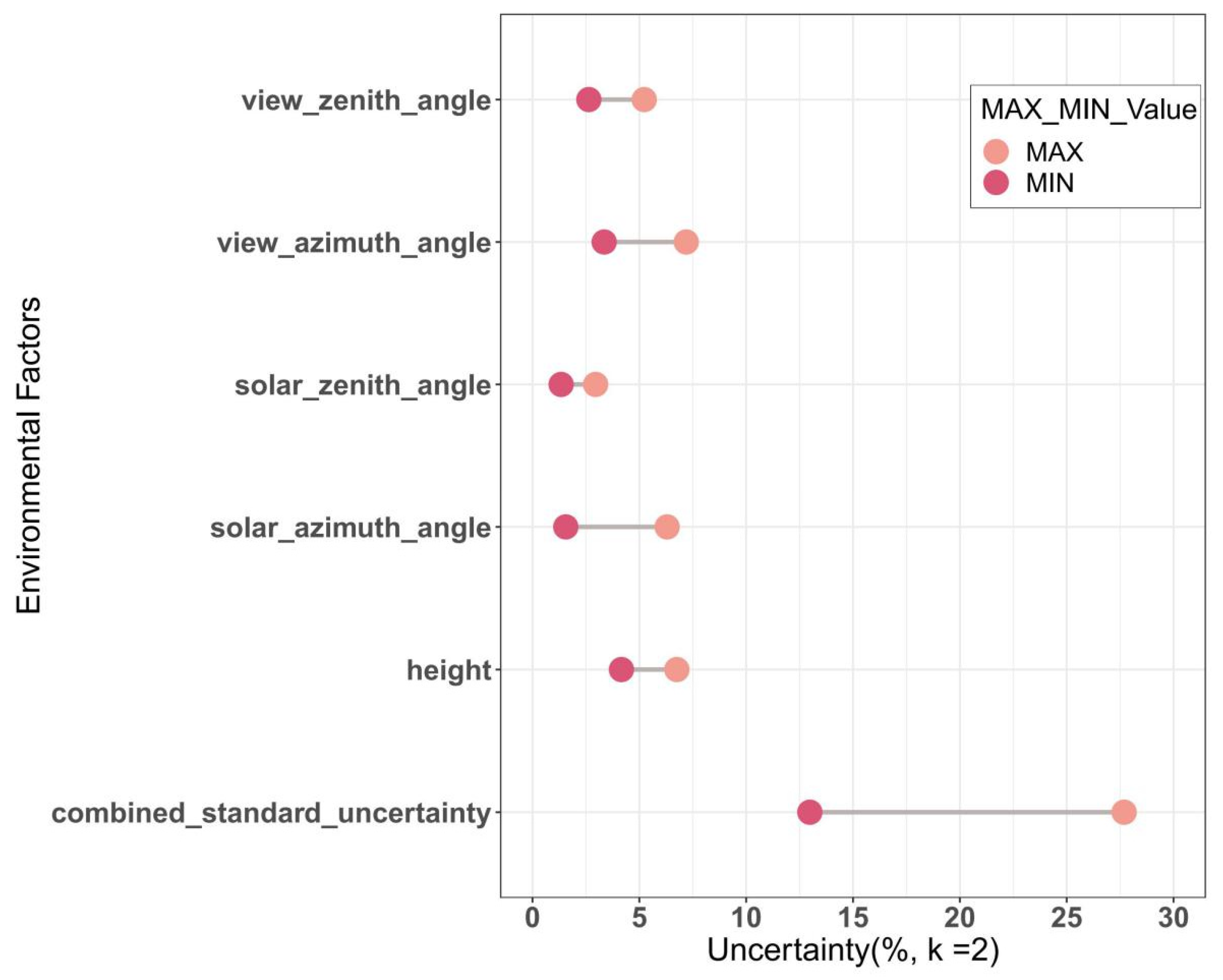
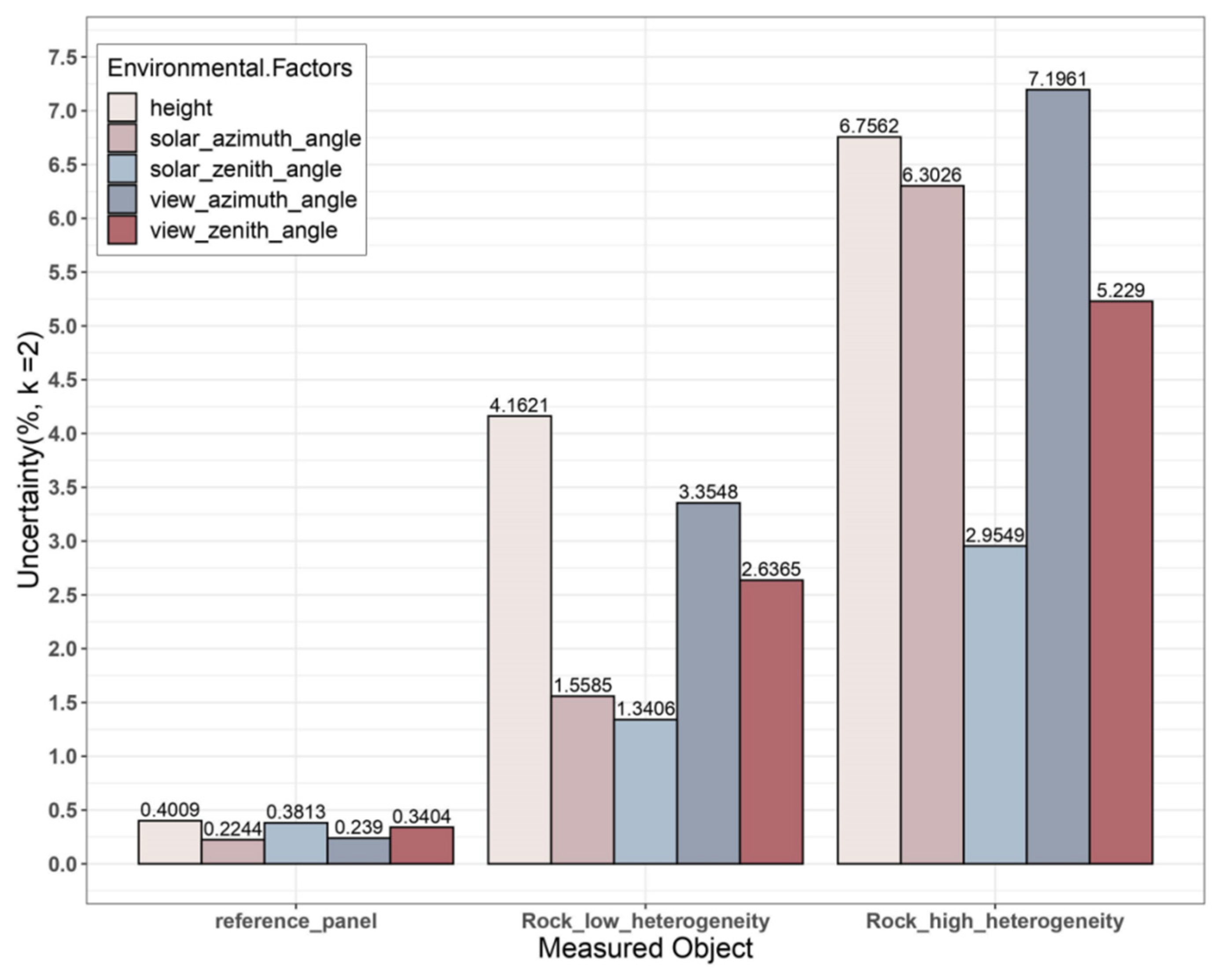
4.1. Uncertainty Analysis of Field Spectral Reflectance Caused by I&VG

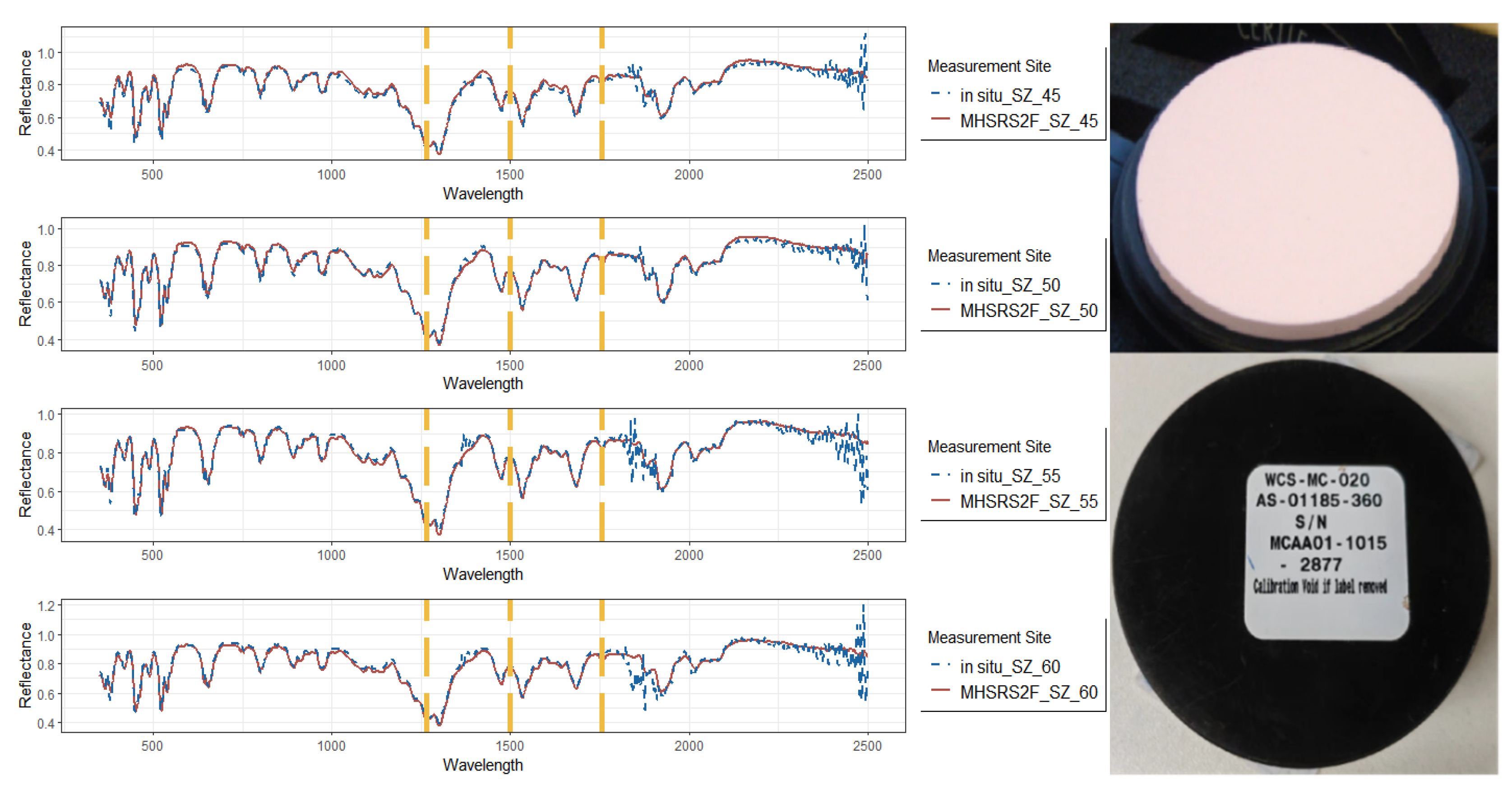
4.1.1. Reference Panel

The reference panel used is the SpectralonTM White Diffuse Reflectance Standard (99%), which is considered as an ideal diffuse reflectance reference surface. Therefore, this article uses the variation in the spectral reflectance for the reference panel under different I&VG conditions to characterize the influence of different I&VG conditions on the spectral reflectance. The uncertainty in the reference panel caused by a single I&VG parameter and the coupling of multiple parameters are calculated and shown in Table 3. A box-plot is used to compare the magnitude of uncertainty (Figure 7).
The comparison results in Figure 7 reveal that the uncertainty of reflectance caused by the observation height is the highest, because it involves the area of the measured object detected using the spectroradiometer. Simultaneously, the uncertainty caused by the solar zenith angle is the second highest, because changes in the solar zenith angle directly affect the magnitude of solar irradiance. In addition, the uncertainty caused by the solar azimuth angle is the lowest. Another noteworthy phenomenon is that the uncertainty caused by the azimuth angle is significantly lower than that of zenith angle. The main reason may be that the surface of the reference panel is a Lambertian and the different view and solar azimuth angles have relatively little influence on spectral reflectance. The above findings indicate that attention should be paid to selecting and unifying the most suitable observation height, viewing direction, and time of spectrum acquisition during field operations.

4.1.2. Rock Samples

In this section, the variation in reflectance of rock samples under different I&VG conditions is used to explore the uncertainty caused by I&VG at different degrees of surface heterogeneity. The uncertainty range caused by a single I&VG parameter and the coupling of multiple parameters for 10 rock samples are presented in Table 4. A dumbbell plot is used to represent the distribution of the uncertainty range (Figure 8). The dumbbell plot reflects the consistency of uncertainty caused by I&VG on 10 rock samples. When the uncertainty range is small, it indicates that the uncertainties caused by I&VG on 10 rock samples are either very large or very small. On the contrary, a large uncertainty range indicates that I&VG has higher uncertainty for some rock samples, while it has lower uncertainty for others.
According to Figure 8, it is apparent that the uncertainty range and value of rock samples caused by the solar zenith angle is the smallest. This indicates that for most rock samples, the uncertainty caused by the solar zenith angle is the smallest. Another finding is that the uncertainty range caused by observation height is relatively small, but the uncertainty value is relatively high. This shows that for most rock samples, the uncertainty caused by the observation height is relatively high. In addition, the uncertainty range caused by the solar and view azimuth angles is the largest. This indicates that for some rock samples, the uncertainty caused by azimuth angle is high, while for other rock samples, the uncertainty caused by azimuth angle is very low. And the uncertainty caused by azimuth angle depends more on the surface heterogeneity of the rock samples. From the above analysis, it can be seen that when there is heterogeneity on the surface, it is necessary to reasonably select and determine the observation height, the direction of sunlight incidence, and the viewing direction.

4.1.3. Comparison of Reference Panel and Rock Samples

According to the surface heterogeneity simulation experiment (see Section 2.4), two rock samples with the highest and lowest surface heterogeneity are selected in this section for comparison with the reference panel (DTS21-1 and DTS21-6 seen in Figure 3). The comparison results of the uncertainty caused by single I&VG parameters are shown in Figure 9. Figure 9 shows that the influence of coupling I&VG with the surface heterogeneity of rock samples is much higher than that caused by I&VG alone. Regardless of the surface heterogeneity, the uncertainty caused by the observation height is relatively high.
Another finding is that the uncertainty of the reference panel caused by the solar zenith angle is the second highest. However, when there is heterogeneity on the surface, the uncertainty caused by the solar zenith angle becomes the lowest. This indicates that the uncertainty caused by the coupling of the solar zenith angle with the surface heterogeneity of rocks is smaller than the influence of other I&VG parameters coupling with the surface heterogeneity. The influence of heterogeneity on the solar zenith angle is less than that on other parameters. In addition, with the increase in the heterogeneity of the rock surface, the uncertainty caused by the solar and view azimuth angles is significantly greater than that caused by the zenith angle.
Taken together, the uncertainty caused by different I&VG parameters is closely related to the surface heterogeneity of the object. Regardless of the surface heterogeneity, the selection of the observation height is very important for spectral reflectance. When the surface of the object is approximately Lambertian, the influence of zenith angle is greater than that of the azimuth angle. This means that more attention needs to be paid to the selection of operation time, as well as the unified regulations of the view zenith angle. When the surface heterogeneity increases to a certain extent, the influence of the azimuth angle is greater than that of the zenith angle. It is necessary to pay more attention to the selection and unified regulations of the incident direction of sunlight and the viewing direction.

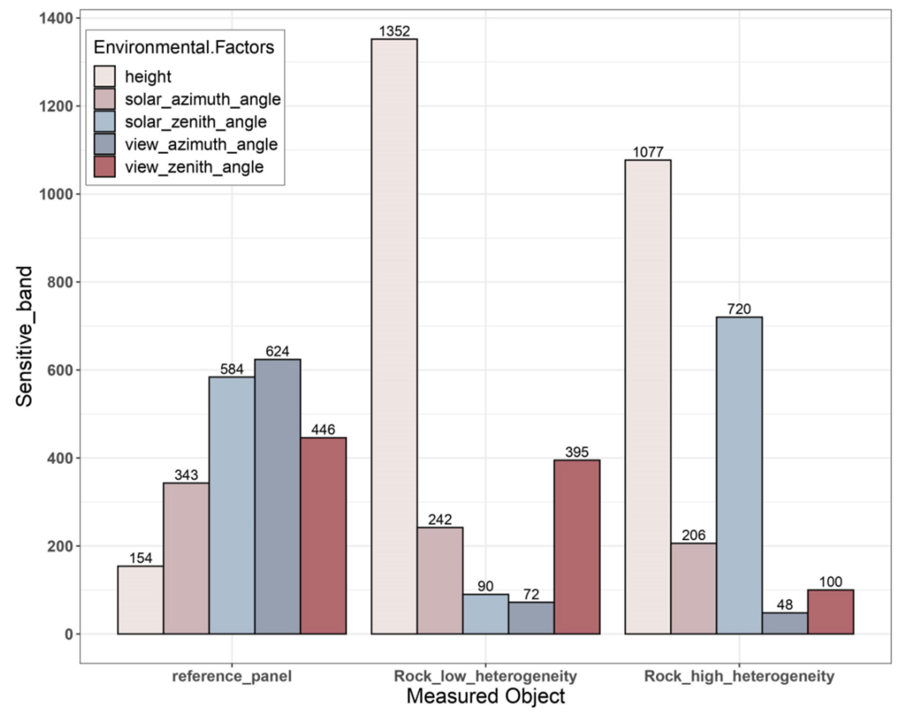
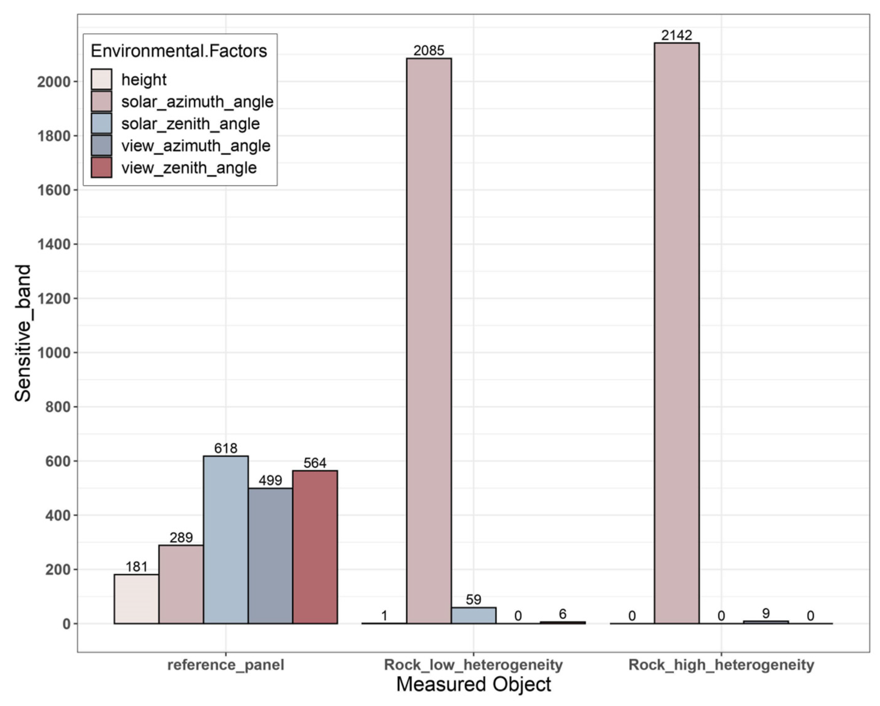
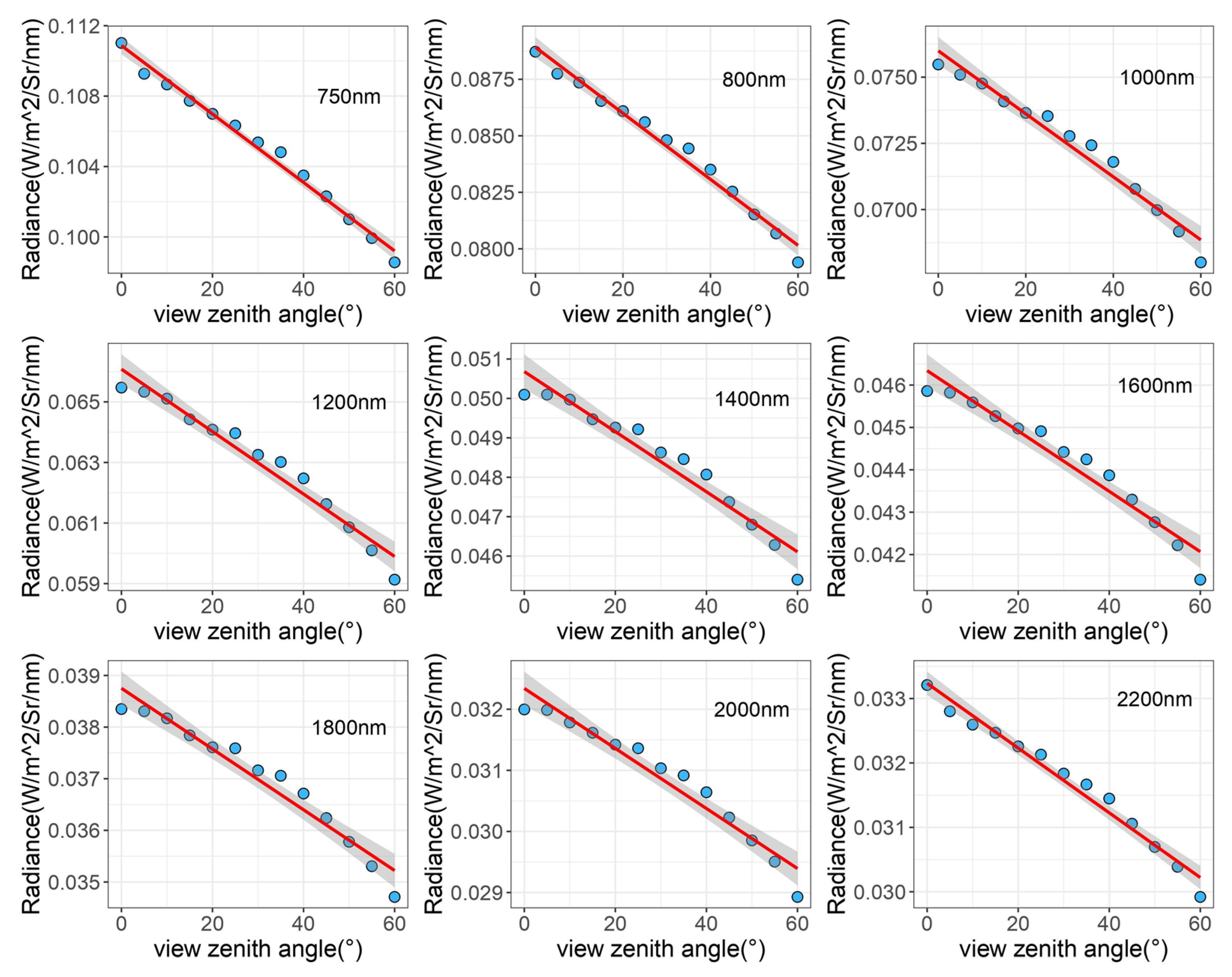
4.2. Sensitivity Analysis of Field Spectral Reflectance to I&VG

4.2.1. First-Order Sensitivity Analysis

In the previous chapter, the uncertainty calculation caused by the coupling of multiple I&VG parameters assumes that the sensitivity of the uncertainty caused by each I&VG parameter on the spectral reflectance uncertainty is consistent. The purpose of this section is to explore the sensitivity of reflectance to each I&VG parameter. The first-order sensitivity coefficient represents the sensitivity of the reflectance data to a single I&VG parameter. Sensitivity analysis still selects the reference panel and the two rock samples with the minimum and maximum heterogeneity as the objects. Since the sensitivity of different bands to I&VG parameters is inconsistent, this work separately counted the most sensitive I&VG parameters for 2150 bands (350 nm–2500 nm) and used a histogram to characterize the number of bands most sensitive to these five I&VG parameters (Figure 10). The comparison results characterize the sensitivity of spectral reflectance to I&VG and the impact of heterogeneity on the first-order sensitivity.
In Figure 10, it can be seen that for the reference panel, the differences between the columns representing the five I&VG parameters are relatively small, which indicates that the sensitivity of each band to I&VG parameters is different. Comparing the histograms of the three measured objects, an interesting phenomenon is that when there is heterogeneity on the surface, the sensitivity of different bands to I&VG begins to show some consistency. The number of bands that are most sensitive to the observation height increases significantly, from minimum to maximum. However, the number of bands that are most sensitive to the view azimuth angle initially changes from maximum to minimum. This reveals that when I&VG parameters are coupled to surface heterogeneity, the reflectance of most bands is more sensitive to observation height than other parameters, but the sensitivity to view azimuth angle is much less than those of the others.
The comparison of the two rock samples in Figure 10 shows that for non-Lambertian objects, the reflectance data are more sensitive to zenith angle than to azimuth angle. When the surface heterogeneity is relatively high, the reflectance is more sensitive to two angles in the direction of sunlight illumination than to two angles in the viewing direction. Another finding is that relatively low surface heterogeneity is more sensitive to the view zenith angle, while relatively high surface heterogeneity is more sensitive to the solar zenith angle.

4.2.2. Total Sensitivity Analysis

Compared to the first-order sensitivity coefficient, the interaction between I&VG parameters is also considered in the total sensitivity coefficient. In this section, the number of bands with the highest total sensitivity coefficients is calculated for the five I&VG parameters for each band of the reference panel and two rock samples (Figure 11). The purpose is to investigate the sensitivity of reflectance at different bands to I&VG after considering the interaction.
Figure 10 and Figure 11 show that, after considering the interaction between different I&VG parameters, most of the bands of two rock samples have changed from being more sensitive to the observation height and zenith angle to being more sensitive to the solar azimuth angle. Since the total sensitivity of each band for the reference panel still has significant differences, it is difficult to analyze the influence of the interactions of I&VG parameters on the sensitivity. Therefore, this section uses a bump chart to characterize the sequence changes in the number of bands that are sensitive to I&VG parameters for the first-order and the total sensitivity coefficients of the reference panel (Figure 12).
Figure 12 shows that the reference panel is the least sensitive to observation height and solar azimuth angle, regardless of whether the interaction between I&VG parameters is considered. This reveals that when the surface of the measured object is close to Lambertian, the slight changes in the observation height and solar azimuth angle have little influence on the reflectance data. Another novel finding is that, for the total sensitivity coefficient, the number of bands sensitive to the zenith angle of the reference panel is greater than that sensitive to the azimuth angle. These results are consistent with the previous uncertainty results of the reference panel caused by I&VG: the uncertainty caused by the zenith angle is greater than by the azimuth angle. The implication of these findings is that the impact of solar and view zenith angles on reflectance is greater than that of solar and view azimuth angles.

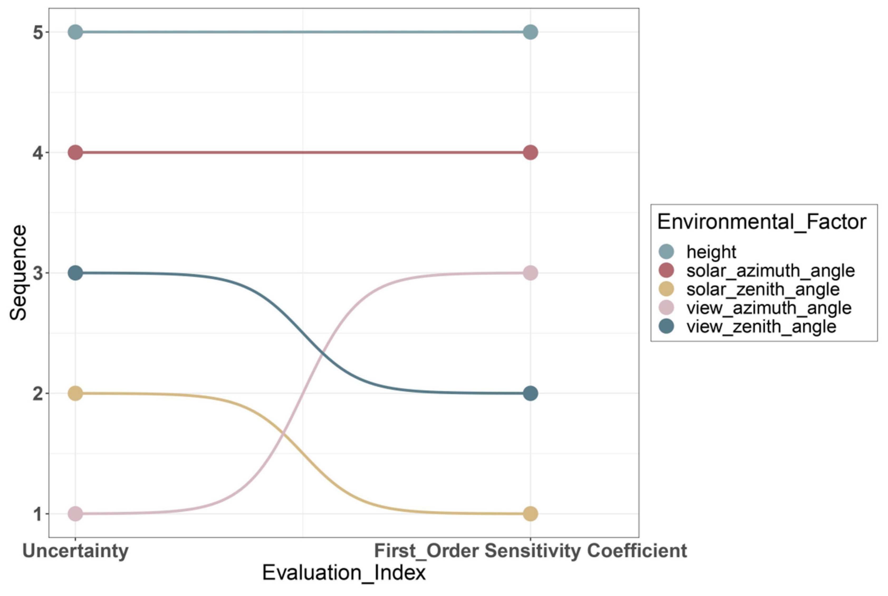
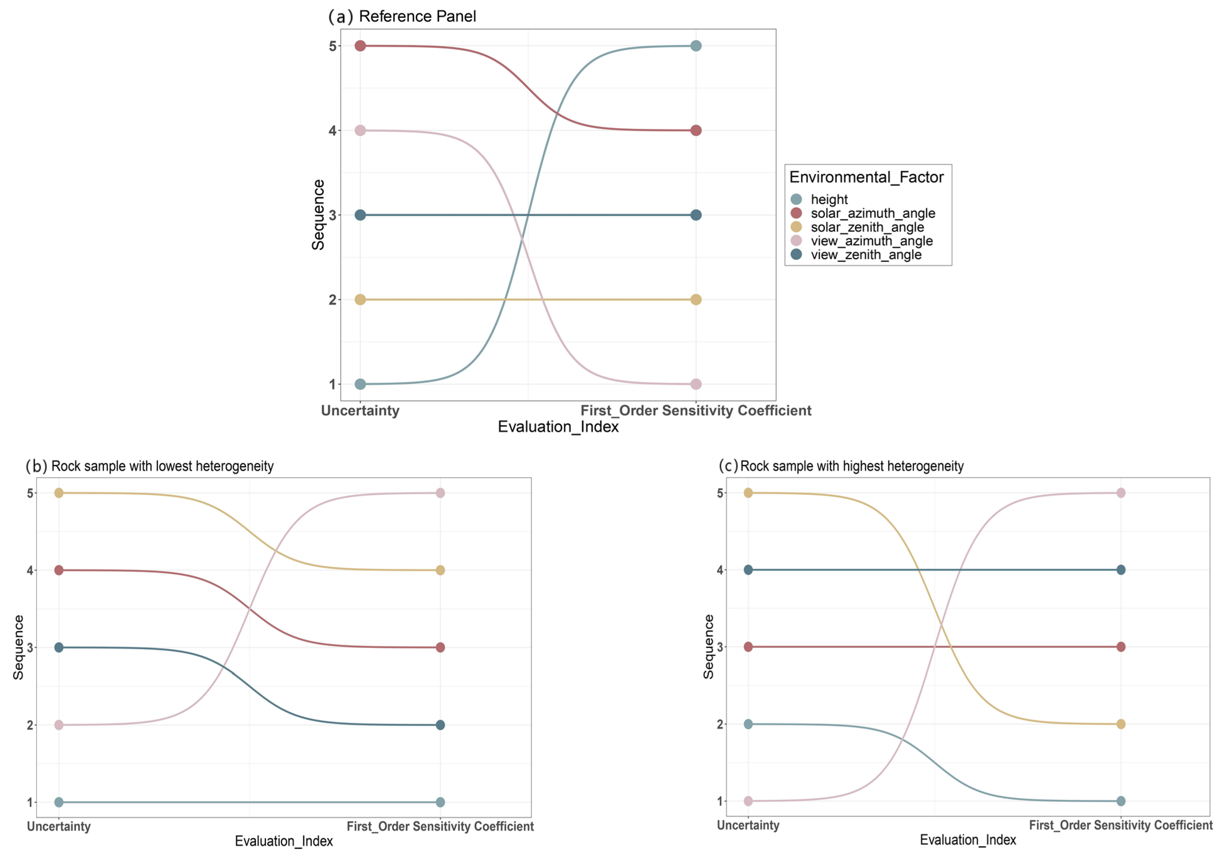
4.2.3. Comparison of First-Order Sensitivity and Uncertainty

The difference between sensitivity and uncertainty is that uncertainty describes the degree of dispersion for the reflectivity of the object within a certain range of I&VG conditions, while sensitivity represents the contribution of various I&VG parameters to the uncertainty of the reflectivity of object. Because the first-order sensitivity coefficient represents the sensitivity to a single I&VG parameter, this section compares the first-order sensitivity coefficient of the reference panel and rock samples with the uncertainty caused by a single I&VG parameter. This section uses a bump chart to characterize the difference between the first-order sensitivity coefficient and the uncertainty caused by a single parameter (Figure 13).
An important finding in Figure 13a is that the uncertainty of the reference panel caused by the observation height is highest, but the reflectance is the least sensitive to the observation height. This discovery reveals that there is a relatively large difference in reflectance collected at observation heights of 20 cm and 100 cm, but the differences between observation heights of several centimeters are small. This means that when objects are close to Lambertian, it is necessary to uniformly specify the observation height, and the influence of the error of several centimeters on the reflectance can be negligible. A further novel finding is that the uncertainty and sensitivity of the solar zenith angle are relatively large. This experimental result definitely supports the need to pay attention to the selection of operation time and changes in the solar zenith angle during in situ measurement. In addition, the uncertainty caused by the view azimuth angle is relatively low, but the sensitivity is highest. This result indicates that when the surface of the object is close to Lambertian, it is necessary to pay attention to changes in the view azimuth angle during the operation process, and slight changes may lead to changes in reflectance.
Comparing these two bump charts in Figure 13b,c, a consistent phenomenon is that the uncertainty and sensitivity caused by the observation height are high regardless of heterogeneity. This reveals that it is necessary to reasonably set a unified observation height and pay attention to slight changes during the spectral acquisition process. It is also worth noting that the uncertainty caused by the solar zenith angle is relatively low, but the sensitivity is relatively high. This indicates that when collecting spectra in situ, it is necessary to pay attention to the instantaneous changes in the solar zenith angle. In addition, the uncertainty caused by the view azimuth angle is relatively high but the sensitivity is the lowest, which means that it is important to carefully consider the viewing direction, but slight changes in the view azimuth angle have little effect on reflectance.

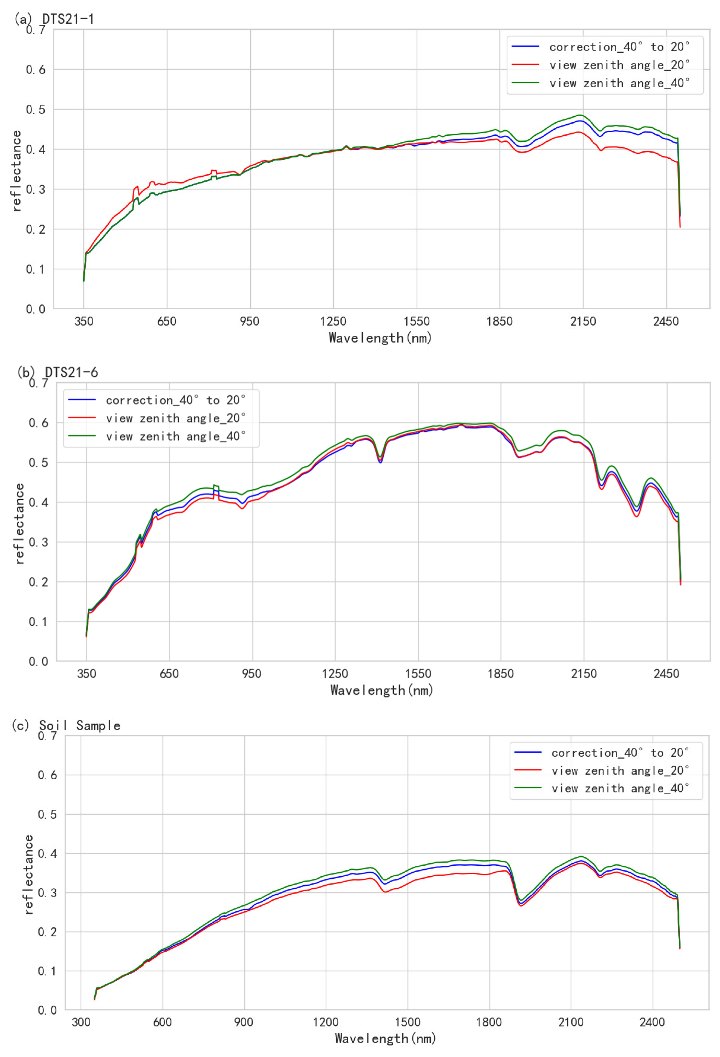
4.3. Correction of Field Data under Different I&VG Conditions

This section conducts reflectance correction work under different I&VG conditions for the 10 rock samples. Figure 14a,b give the correction results for two rock samples from view zenith angles of 40° to 20°. The results of the mean value of the RMSE for 10 rock samples at various wavelengths show that this model has a correction ability of 41.25% for reflectance under different view zenith angles. Moreover, the applicability of this correction model is also tested on soil samples. Figure 14c shows the correction results of a soil sample, and the correction ability can reach 33.9% under different view zenith angles. These results show that this correction model has a good correction effect for reflectance under different view zenith angles.
Compared to the view zenith angle, the correction result of this model for other I&VG parameters is not ideal. The main reason can be attributed to a significant negative linear correlation between the radiance data of the reference panel under different view zenith angles (Figure 15). The average determination coefficient of each band obtained through linear fitting is about 0.9516. However, for the other four I&VG parameters, the goodness of fit of the reference panel radiance under different I&VG parameters is poor or there is no significant trend.
Figure 16a,b show the variation in the radiance of the reference panel under different view and solar azimuth angles. It is worth noting that there is a significant nonlinear correlation between the bands. The correction factors obtained through locally weighted regression do not provide satisfactory correction results for correcting different view and solar azimuth angles. This result can be explained by the fact that most of the blue dots, which represent the measured values, do not fall on the red fitted curve.
Moreover, it can be seen from the red fitted curve in Figure 16c that there is no significant trend in the radiance of different bands under different solar zenith angles. Previous studies have shown that there is only a small correlation between the SD of the reference panel radiance and the solar zenith angle [13], hence the difficulty in correcting the impact of solar zenith angles through the correction factors obtained through curve fitting.
Figure 16d shows the radiance distribution of the reference panel at different observation heights. From the fitting results, it is obviously better than the goodness of fit of azimuth angle. However, the correction model proposed in this paper has little effect on correcting observation heights. One possible explanation for this is that there is a very small difference in the radiance of the reference panel at different observation heights. Therefore, the correction factor is very close to 1, and the correction results for different observation heights through Equation (11) are very small and difficult to observe.

5. Conclusions

In this study, the uncertainty caused by a single I&VG parameter and multiple parameters is quantified (Table 3 and Table 4). The quantification of these uncertainty ranges can provide reference for optimization and improvement of the application of a single truth value based on the object. Uncertainty describes the dispersion of the reflectivity within a certain range of I&VG conditions, while sensitivity represents the influence of slight changes in various I&VG parameters. Therefore, the results of uncertainty and sensitivity analysis can provide the following suggestions and guidance for the optimization design of experimental plans for in situ measurement:
  • The uncertainty and sensitivity caused by different I&VG conditions are closely related to the surface heterogeneity of the object. The greater the surface heterogeneity, the greater the uncertainty.
  • Regardless of surface heterogeneity, the uncertainty and sensitivity caused by observation height are greater than those caused by I&VG. Because the observation height directly affects the size of the field of view and the physicochemical characteristics of the measured object within the field of view, the selection of observation height and the avoidance of changes during the experimental process are crucial. And the scale effect can be a noteworthy issue in the future.
  • For approximate Lambertian objects, the results of uncertainty and sensitivity are relatively consistent. The uncertainty and sensitivity caused by the solar and view zenith angles are relatively high. This indicates that the selection and variation of the zenith angle are crucial.
  • When there is surface heterogeneity on the measured object, the uncertainty caused by the solar and view azimuth angles is relatively high, but it is more sensitive to the solar azimuth angle and solar zenith angle. This indicates that the selection of the solar azimuth angle and the avoidance of changes during the experimental process are crucial. Additionally, more attention should be paid to the changes in the solar zenith angle and the selection of view azimuth angle.
  • The correction method for reflectance data under different I&VG conditions proposed in this study has been successfully applied to correct the view zenith angle and has achieved good results, with a correction ability of 41.25%. However, the correction effect for the other four I&VG parameters is not ideal. Therefore, further exploration of correction models for these I&VG parameters will be required in the future.
Notwithstanding the relatively limited rock samples, this work provides valuable insights into the influence of different I&VG parameters on the spectral reflectance. One of the limitations of this study is the unified use of surface heterogeneity to represent differences in physicochemical properties between objects. The experimental results show that the uncertainty caused by the coupling of surface heterogeneity with I&VG parameters is much greater than that caused by I&VG alone. Therefore, on the basis of understanding the impact of I&VG on spectral reflectance, exploring the impact of coupling different physicochemical properties with I&VG will be a fruitful area for further research. This is helpful for us to better understand the influence mechanism of I&VG for the spectral reflectance of objects.

Author Contributions

Conceptualization, Z.W., G.J. and H.Z.; Methodology, Z.W. and G.J.; Writing—Original Draft, Z.W.; Writing—Review and Editing, G.J. and J.T.; Data Curation, Z.W.; Investigation, S.J.; Resources, S.L.; Visualization, Y.L. All authors have read and agreed to the published version of the manuscript.

Funding

This work is supported by the National Natural Science Foundation of China (61675012).

Data Availability Statement

The data are available from the corresponding author on reasonable request.

Conflicts of Interest

The authors declare no conflict of interest.

Appendix A. Simulation Experiment of Field Environmental Conditions

The purpose of this experiment is to introduce the in situ measurement of rock samples as a standard to verify the simulation degree of field environmental conditions using the MHSRS2F. First, the environmental parameters consistent with Table 1 are set in the MHSRS2F. Then, the atmospheric type of mid-latitude summer and rural aerosol type are simulated through a skylight simulator. Subsequently, the HCRF of rock samples is collected using a reference panel. This study uses two established technologies, the Spectral Angle Mapper (SAM) and Euclidean Distance (ED), as indexes to evaluate the simulation degree of the MHSRS2F to the field environmental conditions. The calculation results indicate that the average value of SAM between the spectra collected based on the MHSRS2F and the in situ measurement can reach 0.9905, and the average value of ED is around 0.2677 (see Table A1). This has verified that the spectral reflectance acquired based on the MHSRS2F is very similar to the in situ measurement.
Table A1. The Spectral Angle Mapper (SAM) and Euclidean Distance (ED) between the HCRF collected based on MHSRS2F and the in situ measurement.
Index
No.
DTS-1DTS-2DTS-3DTS-4DTS-5DTS-6DTS-7DTS-8DTS-9DTS-10
SAM0.99750.98520.98830.98200.99150.99640.98290.99450.99820.9884
ED0.21070.20220.15280.30460.15840.37310.19320.41890.38810.2755
In addition, spectral characteristic parameters are also selected as an index for evaluating spectral consistency in this experiment. And a SpectralonTM Color Diffuse Reflectance Standards panel with absorption characteristics is selected as the measurement object (Figure A1). The HCRF of the reference panel is collected under the same environmental conditions in the field and the MHSRS2F. Three commonly used spectral characteristic parameters, absorption position, absorption depth, and spectral absorption index (SAI), are used to measure the simulation degree of the MHSRS2F to the field environmental conditions. The calculation results indicate that the maximum difference in absorption peak is 2 bands, and the maximum differences in absorption depth and SAI are 0.0159 and 0.01486, respectively (see in Table A2). The above experimental results have verified that the MHSRS2F has a good ability to simulate field environmental conditions.
Table A2. The three popular spectral characteristic parameters used at 1266 nm, 1499 nm, and 1757 nm are compared between the HCRF of the Diffuse Reflectance Standards panel collected based on MHSRS2F and that collected in the field.
Index
Solar Zenith Angle
SZ_45°SZ_50°SZ_55°SZ_60°
In SituHCRFIn SituHCRFIn SituHCRFIn SituHCRF
1266 nmAbsorption Peak12641266126612661266126612671266
Absorption Depth0.56910.55850.56570.56420.56230.56030.55350.5580
Spectral Absorption Index1.06221.18981.21851.20091.20811.18941.04351.1921
1499 nmAbsorption Peak14991498149914991499149814981498
Absorption Depth0.22130.20750.19630.20950.19940.20870.19970.2076
Spectral Absorption Index 1.00721.01311.01591.01501.01391.01431.01571.0120
1757 nmAbsorption Peak17561757175817581757175717581758
Absorption Depth0.15870.14360.12940.14530.13950.14440.13620.1424
Spectral Absorption Index 1.05371.05571.05811.05871.00331.05671.05631.0537
Figure A1. With other environmental conditions unchanged, the HCRF of the reference panel at four solar zenith angles are collected in the field and MHSRS2F. The yellow dashed line shows the three relatively obvious absorption characteristics used for comparison in this section.
Remotesensing 15 05332 g0a1

Appendix B. Instrument and Illumination Stability Experiment

The main focus of this experiment is to verify that the MHSRS2F can maintain the stability of illumination conditions for a long time. According to the experimental scheme in Table A3, the spectra of rock samples are collected every 2 min for 1 h. The environmental conditions of the MHSRS2F are kept unchanged during the experiment. This study uses the root-mean-square error (RMSE) to characterize the reproducibility of the MHSRS2F. It turns out that the reproducibility of the MHSRS2F is between 0.028% and 0.059%. Milton et al. found that under temperate-latitude clear-sky conditions, the reproducibility of continuous-reflectance measurement using the single spectrometer approach is around 7%, and the reproducibility of the dual spectrometer approach is about 3% [28]. Comparison shows that the reproducibility of the single spectrometer approach based on the MHSRS2F is significantly better than the reproducibility of the single spectrometer and dual spectrometer approach in the field.
Table A3. Three groups of stability experiments were conducted, and the environmental condition parameters set for the experiment were as follows.
Experiment No.Sample No.Atmospheric TypeAerosol TypeSolar
Zenith Angle
View
Zenith Angle
Relative
Azimuth Angle
Observation Height
1DTS21-1mid-latitude summerrural aerosol type20°180°100 cm
2DTS21-1mid-latitude summerrural aerosol type30°180°100 cm
3DTS21-1mid-latitude summerrural aerosol type40°180°100 cm

References

  1. Milton, E.J.; Schaepman, M.E.; Anderson, K.; Kneubühler, M.; Fox, N. Progress in field spectroscopy. Remote Sens. Environ. 2009, 113, S92–S109. [Google Scholar] [CrossRef]
  2. Milton, E.J.; Rollin, E.M. Estimating the irradiance spectrum from measurements in a limited number of spectral bands. Remote Sens. Environ. 2006, 100, 348–355. [Google Scholar] [CrossRef]
  3. Brown, L.A.; Camacho, F.; García-Santos, V.; Origo, N.; Fuster, B.; Morris, H.; Pastor-Guzman, J.; Sánchez-Zapero, J.; Morrone, R.; Ryder, J.; et al. Fiducial reference measurements for vegetation bio-geophysical variables: An end-to-end uncertainty evaluation framework. Remote Sens. 2021, 13, 3194. [Google Scholar] [CrossRef]
  4. Buman, B.; Hueni, A.; Colombo, R.; Cogliati, S.; Celesti, M.; Julitta, T.; Burkart, A.; Siegmann, B.; Rascher, U.; Drusch, M.; et al. Towards consistent assessments of in situ radiometric measurements for the validation of fluorescence satellite missions. Remote Sens. Environ. 2022, 274, 112984. [Google Scholar] [CrossRef]
  5. Hadley, B.C.; Garcia-Quijano, M.; Jensen, J.R.; Tullis, J.A. Empirical versus model—based atmospheric correction of digital airborne imaging spectrometer hyperspectral data. Geocarto Int. 2005, 20, 21–28. [Google Scholar] [CrossRef]
  6. Wang, Y.; Leng, P.; Peng, J.; Marzahn, P.; Ludwig, R. Global assessments of two blended microwave soil moisture products CCI and SMOPS with in-situ measurements and reanalysis data. Int. J. Appl. Earth Obs. Geoinf. 2021, 94, 102234. [Google Scholar] [CrossRef]
  7. Fowler, J.; Waldner, F.; Hochman, Z. All pixels are useful, but some are more useful: Efficient in situ data collection for crop-type mapping using sequential exploration methods. Int. J. Appl. Earth Obs. Geoinf. 2020, 91, 102114. [Google Scholar] [CrossRef]
  8. Xu, C.; Qu, J.J.; Hao, X.; Zhu, Z.; Gutenberg, L. Surface soil temperature seasonal variation estimation in a forested area using combined satellite observations and in-situ measurements. Int. J. Appl. Earth Obs. Geoinf. 2020, 91, 102156. [Google Scholar] [CrossRef]
  9. Kraatz, S.; Jacobs, J.M.; Schröder, R.; Cho, E.; Miller, H.J.; Vuyovich, C.M. Improving SMAP freeze-thaw retrievals for pavements using effective soil temperature from GEOS-5: Evaluation against in situ road temperature data over the US. Remote Sens. Environ. 2020, 237, 111545. [Google Scholar] [CrossRef]
  10. Jiménez, M.; de la Cámara, O.G.; Moncholí, A.; Muñoz, F. Towards a complete spectral reflectance uncertainty model for Field Spectroscopy. In Fifth Recent Advances in Quantitative Remote Sensing; Universitat de València: Valencia, Spain, 2018; p. 21. [Google Scholar]
  11. Origo, N.; Gorroño, J.; Ryder, J.; Nightingale, J.; Bialek, A. Fiducial Reference Measurements for validation of Sentinel-2 and Proba-V surface reflectance products. Remote Sens. Environ. 2020, 241, 111690. [Google Scholar] [CrossRef]
  12. Pflug, B.; Louis, J.; de los Reyes, R.; Pflug, K.; Mueller-Wilm, U.; Quang, C.; Iannone, R.Q.; Reinartz, P. Evaluation of SEN2COR surface reflectance products over land surface with reference measurements on ground. In Proceedings of the IGARSS 2022—2022 IEEE International Geoscience and Remote Sensing Symposium, Kuala Lumpur, Malaysia, 17–22 July 2022; pp. 4308–4311. [Google Scholar] [CrossRef]
  13. Wu, X.; Wen, J.; Xiao, Q.; Liu, Q.; Peng, J.; Dou, B.; Li, X.; You, D.; Tang, Y.; Liu, Q. Coarse scale in situ albedo observations over heterogeneous snow-free land surfaces and validation strategy: A case of MODIS albedo products preliminary validation over northern China. Remote Sens. Environ. 2016, 184, 25–39. [Google Scholar] [CrossRef]
  14. Qiu, X.; Jia, G.; Zhao, H.; Zhang, C. Antinoise estimation of temperature and emissivity for FTIR spectrometer data using spectral polishing filters: Design and comparison. IEEE Trans. Geosci. Remote Sens. 2020, 59, 3292–3308. [Google Scholar] [CrossRef]
  15. Biliouris, D.; Verstraeten, W.W.; Dutré, P.; Van Aardt, J.A.; Muys, B.; Coppin, P. A compact laboratory spectro-goniometer (CLabSpeG) to assess the BRDF of materials. Presentation, calibration and implementation on Fagus sylvatica L. Sensors 2007, 7, 1846–1870. [Google Scholar] [CrossRef] [PubMed]
  16. Ji, C.; Bachmann, M.; Esch, T.; Feilhauer, H.; Heiden, U.; Heldens, W.; Hueni, H.; Lakes, T.; Metz-Marconcini, A.; Schroedter-Homscheidt, M.; et al. Solar photovoltaic module detection using laboratory and airborne imaging spectroscopy data. Remote Sens. Environ. 2021, 266, 112692. [Google Scholar] [CrossRef]
  17. Peltoniemi, J.; Hakala, T.; Suomalainen, J.; Puttonen, E. Polarised bidirectional reflectance factor measurements from soil, stones, and snow. J. Quant. Spectrosc. Radiat. Transf. 2009, 110, 1940–1953. [Google Scholar] [CrossRef]
  18. Zhao, F.; Li, Y.; Dai, X.; Verhoef, W.; Guo, Y.; Shang, H.; Gu, X.; Huang, Y.; Yu, T.; Huang, J. Simulated impact of sensor field of view and distance on field measurements of bidirectional reflectance factors for row crops. Remote Sens. Environ. 2015, 156, 129–142. [Google Scholar] [CrossRef]
  19. Gu, X.F.; Guyot, G.; Verbrugghe, M. Evaluation of measurement errors in ground surface reflectance for satellite calibration. Int. J. Remote Sens. 1992, 13, 2531–2546. [Google Scholar] [CrossRef]
  20. Anderson, K.; Milton, E.J. On the temporal stability of ground calibration targets: Implications for the reproducibility of remote sensing methodologies. Int. J. Remote Sens. 2006, 27, 3365–3374. [Google Scholar] [CrossRef]
  21. Anderson, K.; Dungan, J.L.; MacArthur, A. On the reproducibility of field-measured reflectance factors in the context of vegetation studies. Remote Sens. Environ. 2011, 115, 1893–1905. [Google Scholar] [CrossRef]
  22. Zhao, H.; Cui, B.; Jia, G.; Li, N.; Li, X.; Gan, F.; Yu, J. Acquirement of anisotropy reflectance with the multi-directional hyperspectral remote sensing simulation facility (MHSRS2F). Opt. Express 2019, 27, 28760–28781. [Google Scholar] [CrossRef]
  23. ASD. ASD Technical Guide, 3rd ed.; Analytical Spectral Devices, Inc.: Boulder, CO, USA, 1999; pp. 1–140. Available online: https://gep.uchile.cl/Biblioteca/radiometr%C3%ADa%20de%20campo/TechGuide.pdf (accessed on 6 August 2023).
  24. Sobol, I.M. Global sensitivity indices for nonlinear mathematical models and their Monte Carlo estimates. Math. Comput. Simul. 2001, 55, 271–280. [Google Scholar] [CrossRef]
  25. Saltelli, A.; Tarantola, S.; Chan, K.S. A quantitative model-independent method for global sensitivity analysis of model output. Technometrics 1999, 41, 39–56. [Google Scholar] [CrossRef]
  26. Nicodemus, F.E.; Richmond, J.C.; Hsia, J.J.; Ginsberg, I.W.; Limperis, T.; Harman, S.; Baruch, J.J. Geometrical considerations and nomenclature for reflectance. In Final Report National Bureau of Standards; US Department of Commerce, National Bureau of Standards: Washington, DC, USA, 1977; Volume 160, p. 52. [Google Scholar] [CrossRef]
  27. Schaepman-Strub, G.; Schaepman, M.E.; Painter, T.H.; Dangel, S.; Martonchik, J.V. Reflectance quantities in optical remote sensing—Definitions and case studies. Remote Sens. Environ. 2006, 103, 27–42. [Google Scholar] [CrossRef]
  28. Milton, E.J. Review article principles of field spectroscopy. Remote Sens. 1987, 8, 1807–1827. [Google Scholar] [CrossRef]
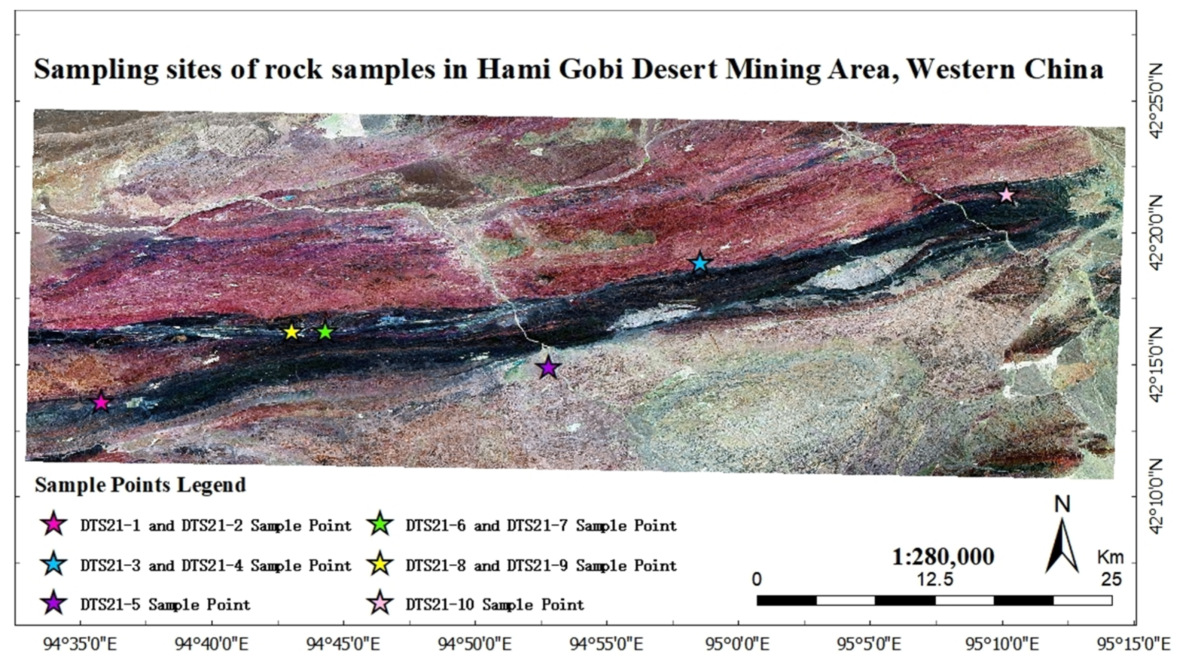
Figure 1. Actual picture of the components and structure of MHSRS2F.
Remotesensing 15 05332 g001
Figure 2. The 10 rock samples were collected from 6 sampling sites in the Gobi Desert Mining Area in the west of Hami City, Xinjiang Uygur Autonomous Region, China. The 6 sampling sites are represented by colored five-pointed stars.
Remotesensing 15 05332 g002
Figure 3. The 10 original-state rock samples used in this experiment.
Remotesensing 15 05332 g003
Figure 4. Adjustment trajectories of different I&VG parameters in the MHSRS2F.
Remotesensing 15 05332 g004
Figure 5. The observation range for heterogeneity evaluation of the sample is shown in the red box (20 cm × 12 cm). The red dots indicate the 45 observation positions at intervals of 2 cm.
Remotesensing 15 05332 g005
Figure 6. Scatter charts with different colors and shapes indicate the uncertainty of the reference panel at different wavelengths with different I&VG parameters. Solid lines of different colors represent the average uncertainty of different wavelengths.
Remotesensing 15 05332 g006
Figure 7. The box-plot shows the uncertainty distribution of the reference panel within the 400–900 nm range, and the red cross represents the average value.
Remotesensing 15 05332 g007
Figure 8. The dumbbell plot shows the uncertainty range of 10 rock samples at different single I&VG parameters and coupling of multiple parameters.
Remotesensing 15 05332 g008
Figure 9. Comparison of the uncertainty caused by five I&VG parameters for the reference panel and two rock samples (k = 2). “Rock_low_heterogeneity” and “Rock_high_heterogeneity” represent the two rock samples DTS21-6 and DTS21-1 with the lowest and highest heterogeneity, respectively.
Remotesensing 15 05332 g009
Figure 10. Comparison of the number of bands with the highest first-order sensitivity coefficient to five I&VG parameters for each band of the reference panel and two rock samples. “Rock_low_heterogeneity” and “Rock_high_heterogeneity” represent the two rock samples DTS21-6 and DTS21-1 with the lowest and highest heterogeneity, respectively.
Remotesensing 15 05332 g010
Figure 11. Comparison of the number of bands with the highest total sensitivity coefficient to five I&VGs for each band of the reference panel and two rock samples. “Rock_low_heterogeneity” and “Rock_high_heterogeneity” represent the two rock samples DTS21-6 and DTS21-1 with the lowest and highest heterogeneity, respectively.
Remotesensing 15 05332 g011
Figure 12. Comparison of sequential changes in the first-order and total sensitivity coefficients of the reference panel for the five I&VG parameters. The sequence from 1 to 5 ranges from the most sensitive to the least sensitive.
Remotesensing 15 05332 g012
Figure 13. Comparison between first-order sensitivity coefficients and uncertainties caused by a single I&VG parameter for reference panel and rock samples. (a) Reference panel, (b) rock sample (DTS21-6) with lowest heterogeneity, (c) rock sample (DTS21-1) with highest heterogeneity. The sequence from 1 to 5 ranges from the most sensitive to the least sensitive.
Remotesensing 15 05332 g013
Figure 14. Correction results of spectral reflectance from view zenith angles of 40° to 20°. (a) Rock sample DTS21-1, (b) rock sample DTS21-6, (c) soil sample. These spectra are consistent in other I&VG conditions except for the view zenith angle.
Remotesensing 15 05332 g014
Figure 15. Reflected radiance of reference panel at different wavelengths as a function of view zenith angle with other I&VG conditions unchanged. The blue dot represents the observation result, the red line represents a fit to the observed results.
Remotesensing 15 05332 g015
Figure 16. Reflected radiance of reference panel at different wavelengths as a function of different I&VG parameters: (a) view azimuth angle, (b) solar azimuth angle, (c) solar zenith solar, (d) observation height. Other I&VG parameter conditions remain unchanged. The blue dot represents the observation result, the red line represents a fit to the observed results.
Remotesensing 15 05332 g016
Table 1. Date, time, location, and environmental conditions for in situ measurements.
Sample No.DateTimeLatitude (°N)Longitude (°E)Solar
Zenith Angle
View
Zenith Angle
Relative
Azimuth Angle
Observation Height
DTS-127 July 202115:1242.225794.598448.5°180°100 cm
DTS-227 July 202114:3542.225794.598442.0°180°100 cm
DTS-312 August 202113:1642.314594.976033.5°180°100 cm
DTS-412 August 202113:1842.314594.976033.5°180°100 cm
DTS-512 August 202114:5442.249094.880148.7°180°100 cm
DTS-614 August 202111:0142.271394.738429.5°180°100 cm
DTS-714 August 202110:5342.271394.738430.0°180°100 cm
DTS-814 August 202116:0042.271294.716861.0°180°100 cm
DTS-914 August 202116:0042.271194.717161.0°180°100 cm
DTS-1014 August 202118:0542.358195.169584.0°180°100 cm
Table 2. Setting of each parameter of I&VG in the simulation experiment of field environmental factors.
Experimental Factors Solar ZenithSolar AzimuthView ZenithView AzimuthObservation HeightAdjust Interval
Solar zenith angle20–60°180°100 cm
Solar azimuth angle20°0–360°180°100 cm10°
View zenith angle20°0–60°180°100 cm
View azimuth angle20°0–360°100 cm10°
Observation height20°180°10 cm–100 cm5 cm
Table 3. Summary of uncertainty results for reference panel, which are caused by five I&VG parameters and the coupling of five parameters (k = 2). The uncertainty caused by a single I&VG parameter is calculated using Equation (4). The combined standard uncertainty refers to the calculations given in Equation (6).
Source of UncertaintyUncertainty (%)
Observation Height0.4009
View Zenith Angle0.3404
View Azimuth Angle0.3604
Solar Zenith Angle0.3813
Solar Azimuth Angle0.2309
Combined Standard Uncertainty0.8579
Table 4. Summary of uncertainty results of the spectral reflectance for rock sample, which are caused by five I&VG parameters and the coupling of five parameters (k = 2). The uncertainty range refers to the calculations given in Equations (5) and (6).
Source of UncertaintyUncertainty Range (%)
Observation Height4.1621–6.7562
View Zenith Angle2.6365–5.2290
View Azimuth Angle3.3548–7.1961
Solar Zenith Angle1.3406–2.9549
Solar Azimuth Angle1.5585–6.3026
Combined Standard Uncertainty12.9801–27.6886
Disclaimer/Publisher’s Note: The statements, opinions and data contained in all publications are solely those of the individual author(s) and contributor(s) and not of MDPI and/or the editor(s). MDPI and/or the editor(s) disclaim responsibility for any injury to people or property resulting from any ideas, methods, instructions or products referred to in the content.

