A Bi-Radial Model for Lens Distortion Correction of Low-Cost UAV Cameras

Abstract

Recently developed cameras in the low-cost sector exhibit lens distortion patterns that cannot be handled well with established models of radial lens distortion. This study presents an approach that divides the image sensor and distortion modeling into two concentric zones for the application of an extended radial lens distortion model. The mathematical model is explained in detail and it was validated on image data from a DJI Mavic Pro UAV camera. First, the special distortion pattern of the camera was examined by decomposing and analyzing the residuals. Then, a novel bi-radial model was introduced to describe the pattern. Eventually, the new model was integrated in a bundle adjustment software package. Practical tests revealed that the residuals of the bundle adjustment could be reduced by 63% with respect to the standard Brown model. On the basis of external reference measurements, an overall reduction in the residual errors of 40% was shown.

1. Introduction

1.1. Pinhole Model

In photogrammetry and computer vision, the pinhole camera model is frequently used to describe the mapping of an object point with world coordinates onto the camera sensor, i.e., the image plane. Figure 1 shows the pinhole model with an image, a camera and the world coordinate system.

Model A describes the corresponding transformation of the object point vector from the world coordinate system into the camera coordinate system (step 1). This is followed by the projection into the image (perspective division, step 2), resulting in the image point given in the camera coordinate system. Afterwards, the image point is shifted into the image coordinate system defined by the image center (step 3).

Model A: Pinhole model

Step 1: ${\overrightarrow{X}}_c={\left(\begin{array}{ccc}{X}_c& Y_c& Z_c\end{array}\right)}^T={\mathbf{R}}^T·({\overrightarrow{X}}_w-{\overrightarrow{X}}_{projC})$ Step 2: $\left(\begin{array}{c}{x}_c\\ y_c\end{array}\right)=-\frac{c}{Z_c}·\left(\begin{array}{c}{X}_c\\ Y_c\end{array}\right)$ Step 3: $\left(\begin{array}{c}{x}_i\\ y_i\end{array}\right)=\left(\begin{array}{c}{x}_p\\ y_p\end{array}\right)+\left(\begin{array}{c}{x}_c\\ y_c\end{array}\right)$

where   ${\overrightarrow{X}}_{\mathit{projC}}$ = center of projection coordinates in world coordinate system

R = rotation matrix of the camera coordinate system

${\overrightarrow{X}}_w$ = (Xw, Yw, Zw)T = object point in world coordinate system

c = principal distance

${\overrightarrow{X}}_c$ = (Xc, Yc, Zc)T = object point in camera coordinate system

${\overrightarrow{x}}_c$ = (xc, yc, −c)T = image point in camera coordinate system

xi, yi = image point in image coordinate system

xp, yp = principal point in image coordinate system

These steps are often summarized in the collinearity equations [1], see Equation (1).

$$\begin{array}{c}{x}_i=x_p-c·\frac{r_{11}·(X_w-X_{projC})+r_{21}·(Y_w-Y_{projC})+r_{31}·(Z_w-Z_{projC})}{r_{13}·(X_w-X_{projC})+r_{23}·(Y_w-Y_{projC})+r_{33}·(Z_w-Z_{projC})}\\ y_i=y_p-c·\frac{r_{12}·(X_w-X_{projC})+r_{22}·(Y_w-Y_{projC})+r_{32}·(Z_w-Z_{projC})}{r_{13}·(X_w-X_{projC})+r_{23}·(Y_w-Y_{projC})+r_{33}·(Z_w-Z_{projC})}\end{array}$$

(1)

where r_kl = elements of the rotation matrix R.

1.2. Lens Distortion

There are several influences that lead to a deviation of the pure pin hole model due to different lens distortions, which are depicted in detail in the following.

1.2.1. Symmetric Radial Lens Distortion

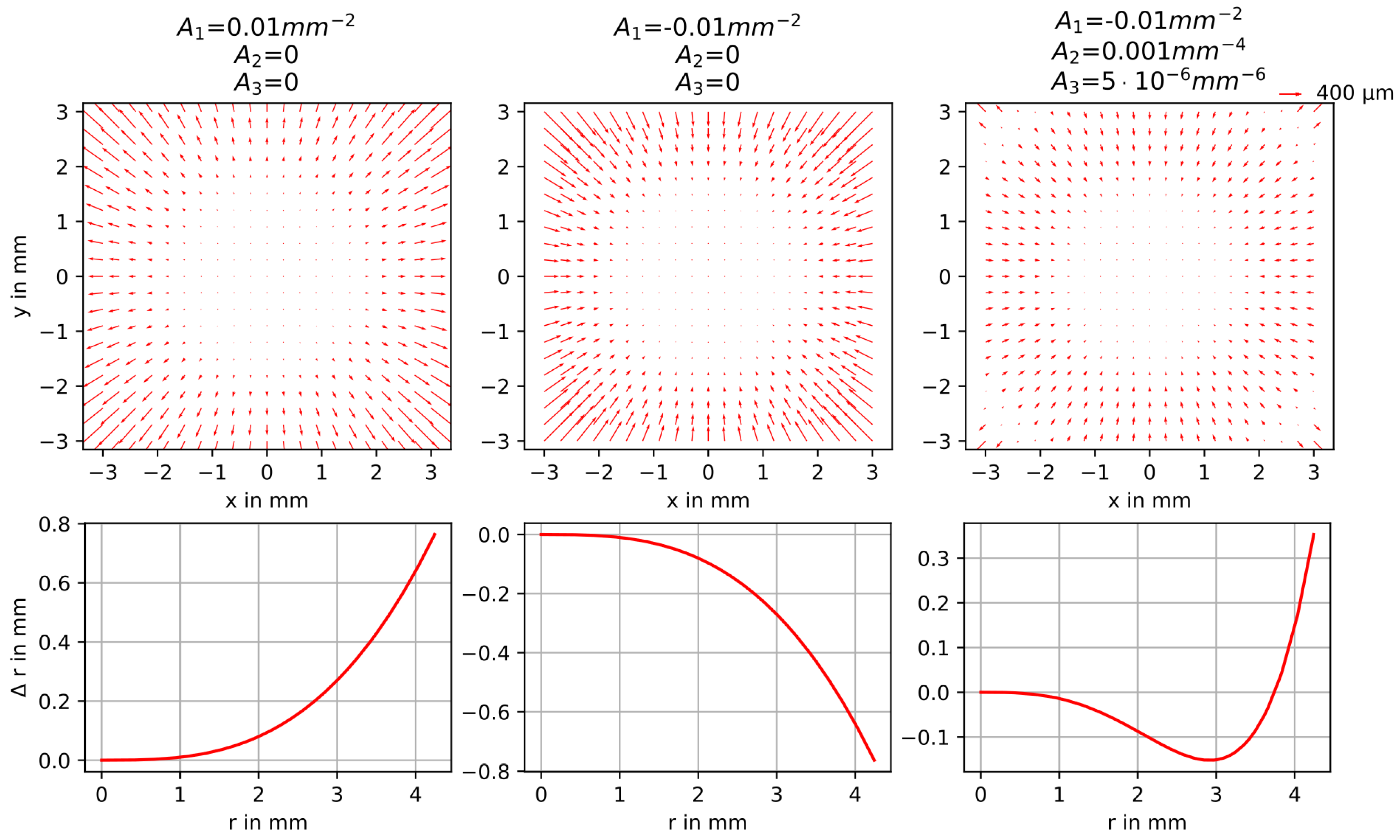
Seidel aberrations [2] of spherical lenses cause symmetric radial image distortions centered around the principal point. This effect leads to different image scales that depend on the distance to the optical axis due to the changing refractive power of the lens. There are two main types of radial distortions that are observable in practice: barrel and pincushion distortion. Brown [3] introduced a correction term, which is a power series applied to the radial distance from the principal point r:

$$\Delta r=A_1·r^3+A_2·r^5+A_3·r^7$$

(2)

where      $r=\sqrt{x_c^2+y_c^2}$ = distance from the principal point;

    Δr = correction term at the distance from the principal point;

    A₁, A₂, A₃ = parameters of radial distortion.

The corrections applied to the coordinates are:

$$\begin{array}{cc}\Delta x_{radial}=& \frac{\Delta r}{r}·x_c\\ \Delta y_{radial}=& \frac{\Delta r}{r}·y_c\end{array}$$

(3)

Figure 2 shows exemplary correction vectors for symmetric radial distortion applying Equation (2).

1.2.2. Decentering Lens Distortion

The decentering of the lens, i.e., due to the misalignment of individual elements of the lens system, also leads to distortions in the image. Conrady [4] analyzed this effect mathematically and could thereby show that there is a tangential as well as an asymmetric radial component, where the latter is three times larger than the former. Therefore, Brown [5] proposed the well-known parameterization that considers four parameters:

$$\begin{array}{c}\Delta x_{decentering}=(B_1·(r^2+2·x_c^2)+2·B_2·x_c·y_c)·(1+B_3·r^2+B_4·r^4)\\ \Delta y_{decentering}=(B_2·(r^2+2·y_c^2)+2·B_1·x_c·y_c)·(1+B_3·r^2+B_4·r^4)\end{array}$$

(4)

where      x_c, y_c = camera coordinates centered at the principal point;

   B₁, B₂, B₃, B₄ = parameters of decentering distortion.

Corrections are often not required in case of high-quality camera systems, and often the model is reduced to two parameters [6] (Equation (5)). Luhmann et al. [6] recommend the decentering distortion model mainly for low-cost or mobile phone cameras.

$$\begin{array}{cc}\Delta x_{decentering}=& B_1·(r^2+2·x_c^2)+2·B_2·x_c·y_c\\ \Delta y_{decentering}=& B_2·(r^2+2·y_c^2)+2·B_1·x_c·y_c\end{array}$$

(5)

Figure 3 shows exemplary correction vectors for decentering distortion applying Equation (5).

1.2.3. Affinity and Non-Orthogonality

In addition to the radial and decentering lens distortions, affine parameters for non-orthogonality and shear are often integrated in standard camera models to overcome effects from camera electronics [7].

Equation (6) shows the correction terms with the two parameters $C_1$ and $C_2$:

$$\begin{array}{cc}\Delta x_{affinity}=& C_1·x_c+C_2·y_c\\ \Delta y_{affinity}=& \hfill 0\hfill \end{array}$$

(6)

1.2.4. Pinhole Model Including Distortion

Eventually, all the previously explained corrections for distortion and affinity can be summarized:

$$\begin{array}{c}\Delta x=\Delta x_{radial}+\Delta x_{decentering}+\Delta x_{affinity}\\ \Delta y=\Delta y_{radial}+\Delta y_{decentering}+\Delta y_{affinity}\end{array}$$

(7)

Consideration of these corrections leads to an extension of the pure pinhole model (model A). The extended model (here called model B) is a widely used model [8].

Model B: Pinhole model including distortion

Step 1: ${\overrightarrow{X}}_c={\left(\begin{array}{ccc}{X}_c& Y_c& Z_c\end{array}\right)}^T={\mathbf{R}}^T·({\overrightarrow{X}}_w-{\overrightarrow{X}}_{projC})$

Step 2: $\left(\begin{array}{c}{x}_c\\ y_c\end{array}\right)=-\frac{c}{Z_c}·\left(\begin{array}{c}{X}_c\\ Y_c\end{array}\right)$

Step 3: $\left(\begin{array}{c}\Delta x\\ \Delta y\end{array}\right)=\frac{\Delta r}{r}·\left(\begin{array}{c}{x}_c\\ y_c\end{array}\right)+\left(\begin{array}{c}{B}_1·(r^2+2·x_c^2)+2·B_2·x_c·y_c+C_1·x_c+C_2·y_c\\ B_2·(r^2+2·y_c^2)+2·B_1·x_c·y_c\end{array}\right)$

with $r=\sqrt{x_c^2+y_c^2}$ and $\Delta r=A_1·r^3+A_2·r^5+A_3·r^7$

Step 4: $\left(\begin{array}{c}{x}_i\\ y_i\end{array}\right)=\left(\begin{array}{c}{x}_p\\ y_p\end{array}\right)+\left(\begin{array}{c}{x}_c\\ y_c\end{array}\right)+\left(\begin{array}{c}\Delta x\\ \Delta y\end{array}\right)$

The corrections can also be integrated into the collinearity equations:

$$\begin{array}{c}{x}_i=x_p-c·\frac{r_{11}·(X_w-X_{projC})+r_{21}·(Y_w-Y_{projC})+r_{31}·(Z_w-Z_{projC})}{r_{13}·(X_w-X_{projC})+r_{23}·(Y_w-Y_{projC})+r_{33}·(Z_w-Z_{projC})}+\Delta x\\ y_i=y_p-c·\frac{r_{12}·(X_w-X_{projC})+r_{22}·(Y_w-Y_{projC})+r_{32}·(Z_w-Z_{projC})}{r_{13}·(X_w-X_{projC})+r_{23}·(Y_w-Y_{projC})+r_{33}·(Z_w-Z_{projC})}+\Delta y\end{array}$$

(8)

1.3. Non-Physical Models for Distortion Corrections

There are distortions that may not be described fully by physically motivated parameters. For this purpose, correction approaches based on mathematical functions only can be used. Thereby, distortion can be, for instance, approximated by polynomials up to a certain order. Mathematical correction approaches with orthogonal, bivariate polynomials of second and fourth order were first presented by Ebner [9] and Grün [10], respectively. These models were mainly intended for application in aerial photogrammetry. More recent approaches are based on polynomial series such as Chebychev polynomials [11], Legendre polynomials [12], or considering Fourier series [13]. A combination of physical and mathematical models is possible as well [14,15]. Some of these approaches consist of a large number of polynomials or parameters and not all of them might be significant. Furthermore, correlations among them may appear, which can lead to a poor convergence behavior of the bundle adjustment.

Physical and mathematical approaches are usually well suited to correcting global distortion patterns. However, local effects may also occur, which can be corrected using the finite element method [14,16] or considering a local distortion model [17]. Luhmann et al. [8] give an overview of the mathematical models and calibration techniques for a wide range of cameras.

1.4. Motivation of This Work

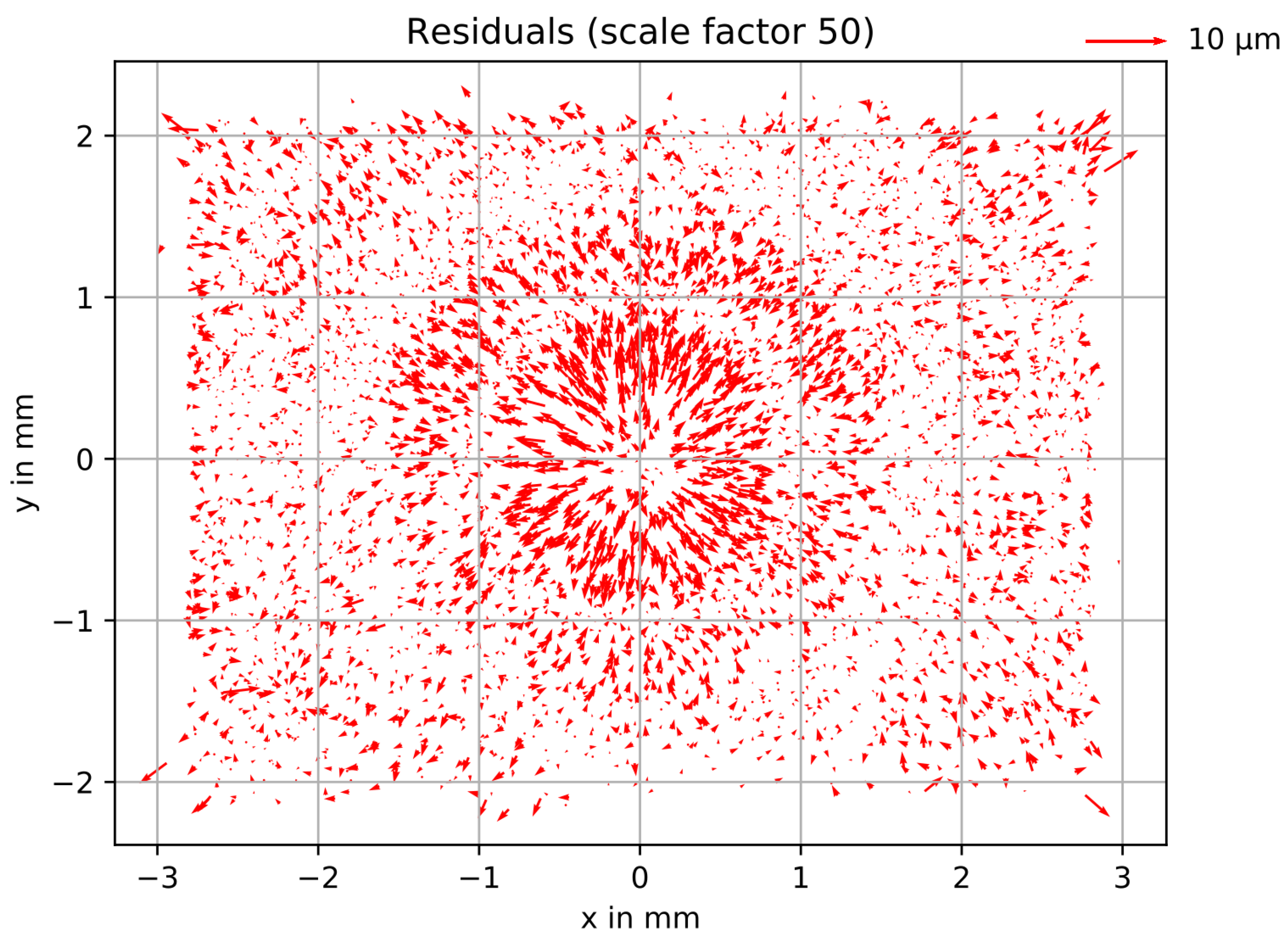
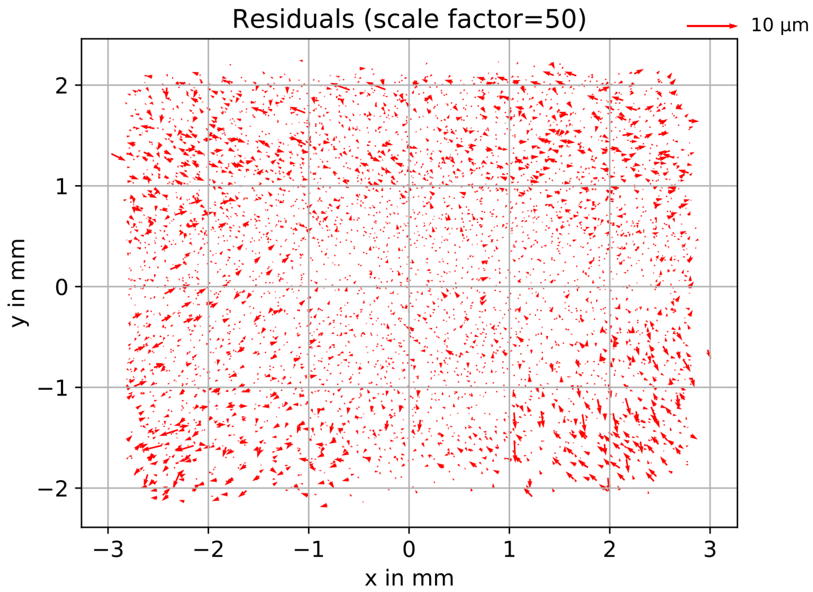
UAV photogrammetry with low-cost cameras is used in a wide range of applications such as archaeology, building modeling, ecology, forestry, hydrology or geomorphology [18]. Some of these low-cost cameras revealed to be challenging to model with the standard distortion models. For instance, Eltner et al. [19] applied the 10-parameter model (model B, based on [3,7]) to a DJI Mavic Pro camera and showed that large errors remained after bundle adjustment, which was indicated by large residuals. Figure 4 visualizes the corresponding residual plot for the residual vectors of all image points that were included in the self-calibration during bundle adjustment. There were unusually large radial deviations around the image center and a clear systematic pattern remained.

Hastedt et al. [15] also studied this type of camera. They suspected that some UAV camera lenses constructed from aspheric lenses may not be made of glass and that there is some internal black box image pre-processing, such as filtering and other corrections, that could lead to this behavior. In addition, ref. [20] highlighted that image pre-processing by the UAV camera manufacturer can result in physically based lens distortion models no longer being valid for actual bundle adjustment because only residual distortion is modeled. Hastedt et al. [15] proposed an extended Brown polynomial to overcome the effects shown in Figure 4.

The article at hand presents an alternative parametrization for radial distortion that is called the bi-radial model. In contrast to existing correction models, the bi-radial approach divides the sensor into two concentric zones in which independent Brown polynomials are applied. Our approach is compared with the method of [15].

The article is structured as follows: First, we analyze the special residual patterns. Thus, the radial components of the residuals are computed and appropriate models are proposed. The results of this analysis are then integrated into a bundle adjustment. Afterwards, the new models are validated. Finally, the results are discussed and concluded.

2. Methods and Results

In this section, we first analyze the results of a bundle adjustment with fixed object coordinates and without considering the distortions of the tested DJI Mavic Pro camera, i.e., by using model A. Then, we introduce a new distortion model (bi-radial distortion correction, Section 2.3), which we integrated in an extended bundle block adjustment to calibrate the DJI Mavic Pro camera (Section 2.4). The results reveal an improved removal of systematic residuals (Section 2.5). To further enhance the bi-radial correction, we also present an automated segmentation of the distortion zones (Section 2.6) and eventually validate the bi-radial distortion correction approach (Section 2.7).

2.1. Analysis of the Residual Patterns

We used a reference target field (Figure 5) to analyze the DJI Mavic Pro camera (see

Table 1. Sensor specifications for the DJI Mavic Pro camera.

Model	DJI Mavic Pro FC220
Sensor size in px	4000 × 3000 px
Sensor size in mm	6.2 mm × 4.65 mm 1
Company	DJI

¹ We assumed a pixel size of 1.55 µm.

). The target field has a size of approximately 7 m × 3 m × 1 m. The reference coordinates of the target field were determined photogrammetrically using an image block captured by a high-quality camera (Panasonic Lumix DMC-GX80 camera (from company Panasonic) with a lens with a focal length of 20 mm) and performing a free bundle adjustment with model B (standard model).

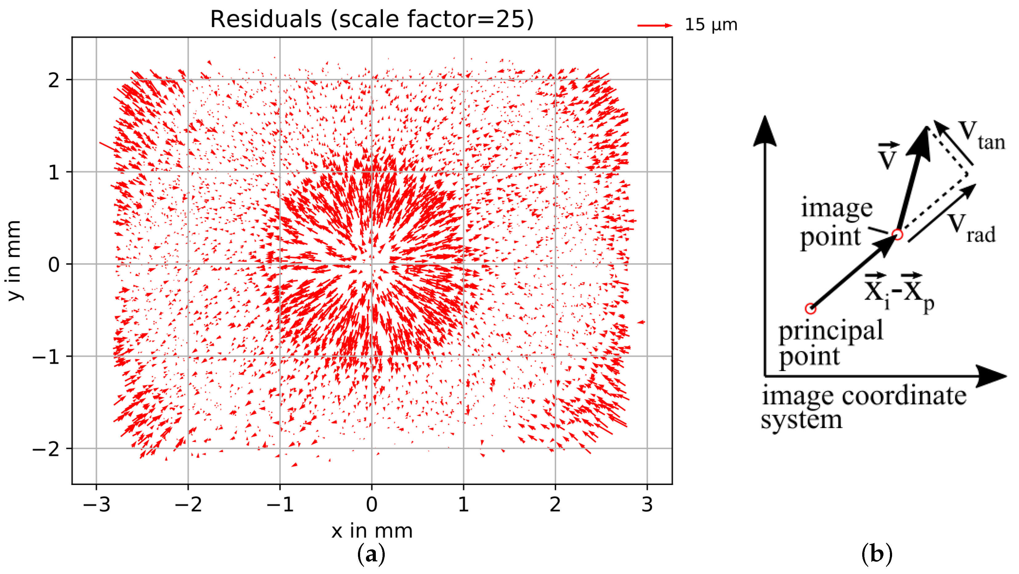
The coordinates, obtained photogrammetically by the data from the Panasonic Lumix DMC-GX80 camera, were used as control points, i.e., they were kept fixed for a second bundle adjustment using an image data set of the reference target field acquired with the DJI Mavic Pro camera (from company DJI). Model A (pinhole model without distortion correction) was applied in the bundle adjustment with the DJI data. This approach was chosen to retrieve the full distortion pattern to identify systematics. The residuals of the image points after the bundle adjustment are depicted as a vector field in Figure 6a, revealing a similar behavior as already shown in Figure 4.

The residual vectors were decomposed into a radial and tangential part (Figure 6b). The radial component was computed by projecting the residual vector onto the difference vector between the principal point and the image point:

$$v_{rad}=\left\{\begin{array}{cc}{\overrightarrow{v}}^T·\frac{{\overrightarrow{x}}_i-{\overrightarrow{x}}_p}{|{\overrightarrow{x}}_i-{\overrightarrow{x}}_p|}\hfill & \mathrm{for}|{\overrightarrow{x}}_i-{\overrightarrow{x}}_p|\ne 0\hfill \\ 0\hfill & \mathrm{otherwise}\hfill \end{array}\right.$$

(9)

where    $\overrightarrow{v}$ = residual vector of the image point;

     ${\overrightarrow{x}}_i$ = image coordinate vector;

     ${\overrightarrow{x}}_p$ = principal point coordinate vector

The tangential component was calculated by the projection of the residual’s normal onto the difference vector:

$$v_{tan}=\left\{\begin{array}{cc}{\left(\begin{array}{c}{v}_y\\ -v_x\end{array}\right)}^T·\frac{{\overrightarrow{x}}_i-{\overrightarrow{x}}_p}{|{\overrightarrow{x}}_i-{\overrightarrow{x}}_p|}\hfill & \mathrm{for}|{\overrightarrow{x}}_i-{\overrightarrow{x}}_p|\ne 0\hfill \\ 0\hfill & \mathrm{otherwise}\hfill \end{array}\right.$$

(10)

where      v_x = x component of the residual vector;

    v_y = y component of the residual vector.

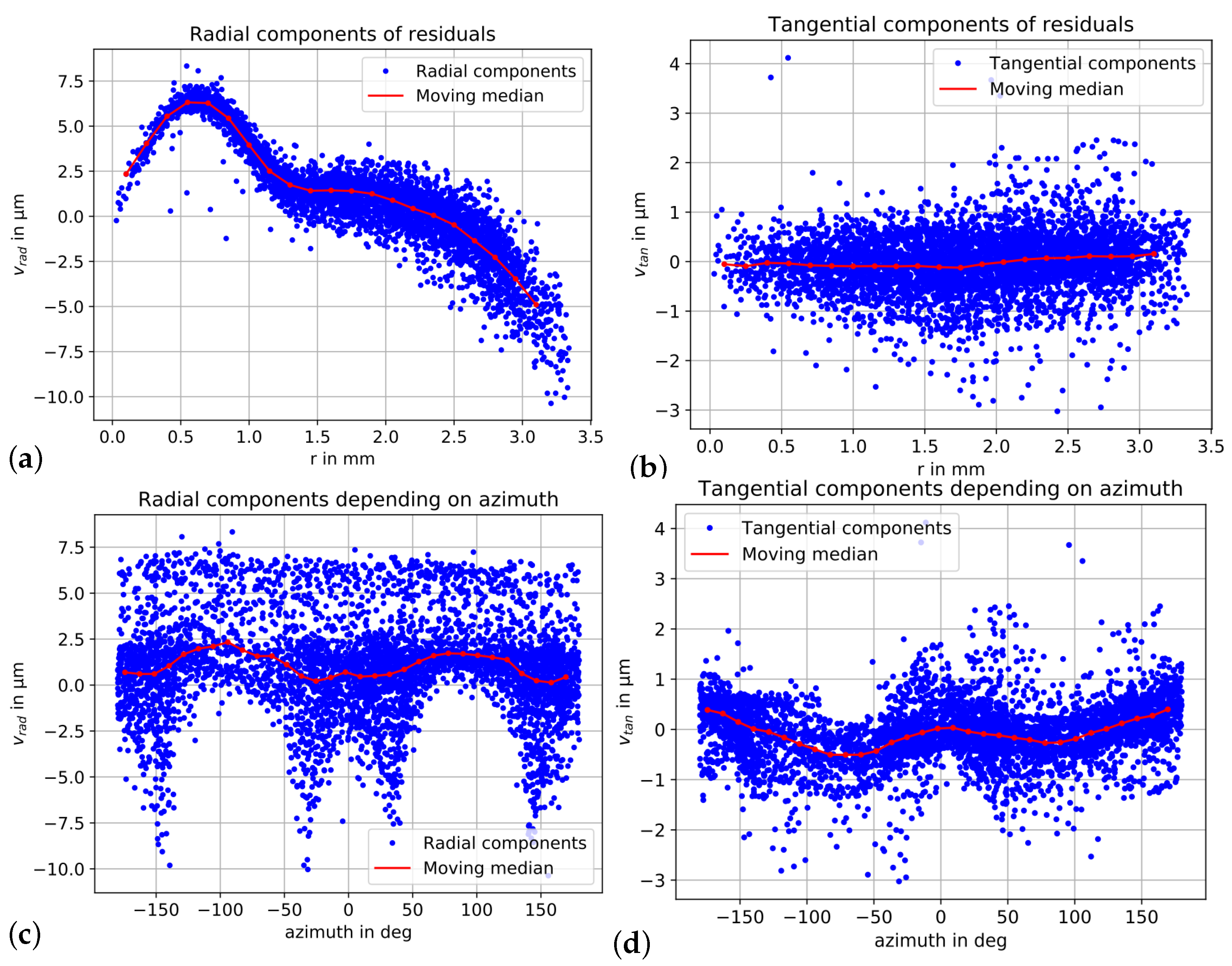
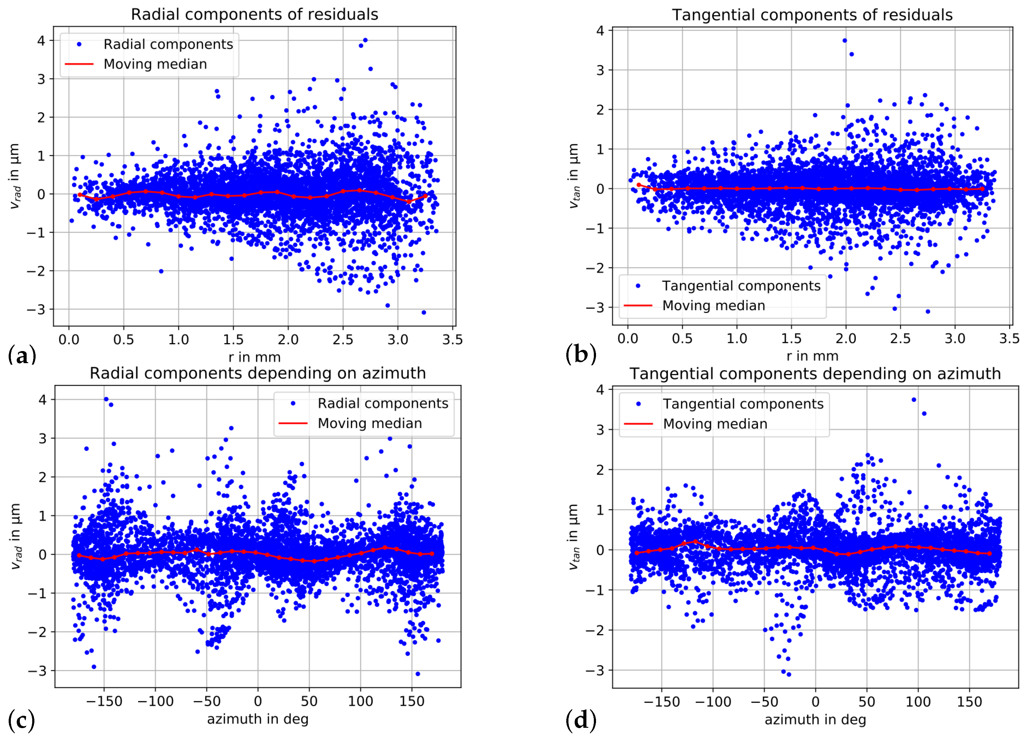
Both components are visualized as a function of the image radius r and as a function of the azimuth of the image point in Figure 7. In addition, the moving median is depicted in red, which was computed using the neighbors around the measurement point in a distance of 0.1 mm. The radial component (over r) shows a strong systematic behavior (Figure 7a), whereas the tangential component appears to be randomly distributed (Figure 7b). Figure 7c,d further reveal a systematic effect for both components regarding the azimuth that may show radial asymmetric effects. However, the radial component also shows a high scattering when considering the azimuth (Figure 7c). Figure 7c also show four vertical tails with larger radial components around the azimuth abscissae of about ±45° and ±135°. These values are caused by the residuals of the image corner points as visible in Figure 6a. In the following, we concentrate on the radial component versus the image radius.

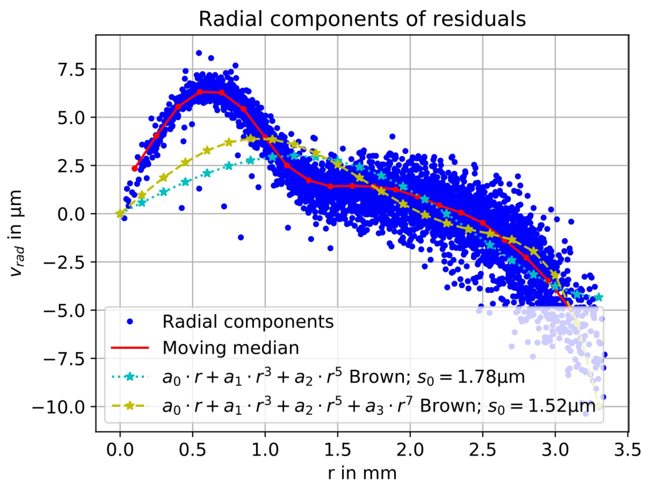
Polynomial fits for the radial components versus image radius shown in Figure 7a were computed using the radial Brown polynomials $\Delta r\left(r\right)=a_0·r+a_1·r^3+a_2·r^5$ and $\Delta r\left(r\right)=a_0·r+a_1·r^3+a_2·r^5+a_3·r^7$. In contrast to the bundle adjustment, the $A_0$ term was included in the polynomial fit to take the influence of the principal distance into account. However, the linear $A_0$ term had to be omitted in the bundle adjustment because it cannot be separated from the principal distance [6]. To evaluate the quality of the polynomial fit, the standard deviation of the unit weight $s_0$ was computed as $s_0=\sqrt{\frac{{\sum }_{i=1}^n{(v_{rad,i}-\Delta r\left(r_i\right))}^2}{n-u}}$ (where n = number of points and u = number of unknowns).

Figure 8 displays the fitted Brown polynomials. Significant deviations of the polynomial to the points in the left part of the curve (corresponding to the central part of the image format) become obvious, explaining the behavior noticed in [19], which is also visible in Figure 6a. The Brown polynomials do not model the behavior of this lens well. The standard deviations of the unit weights $s_0$ of the polynomial fits considering three and four parameters are 1.78 µm (1.15 px) and 1.52 µm (0.98 px), respectively.

2.2. Extended Brown Polynomial Model

The extension of the radial function with even coefficients corresponds to the extended radial polynomial of [15]. We fitted this extended model (Equations (11) and (12)) to our data:

$$\Delta r\left(r\right)=\sum _{i=1}^5{a}_i·r^i$$

(11)

and

$$\Delta r\left(r\right)=\sum _{i=1}^7{a}_i·r^i$$

(12)

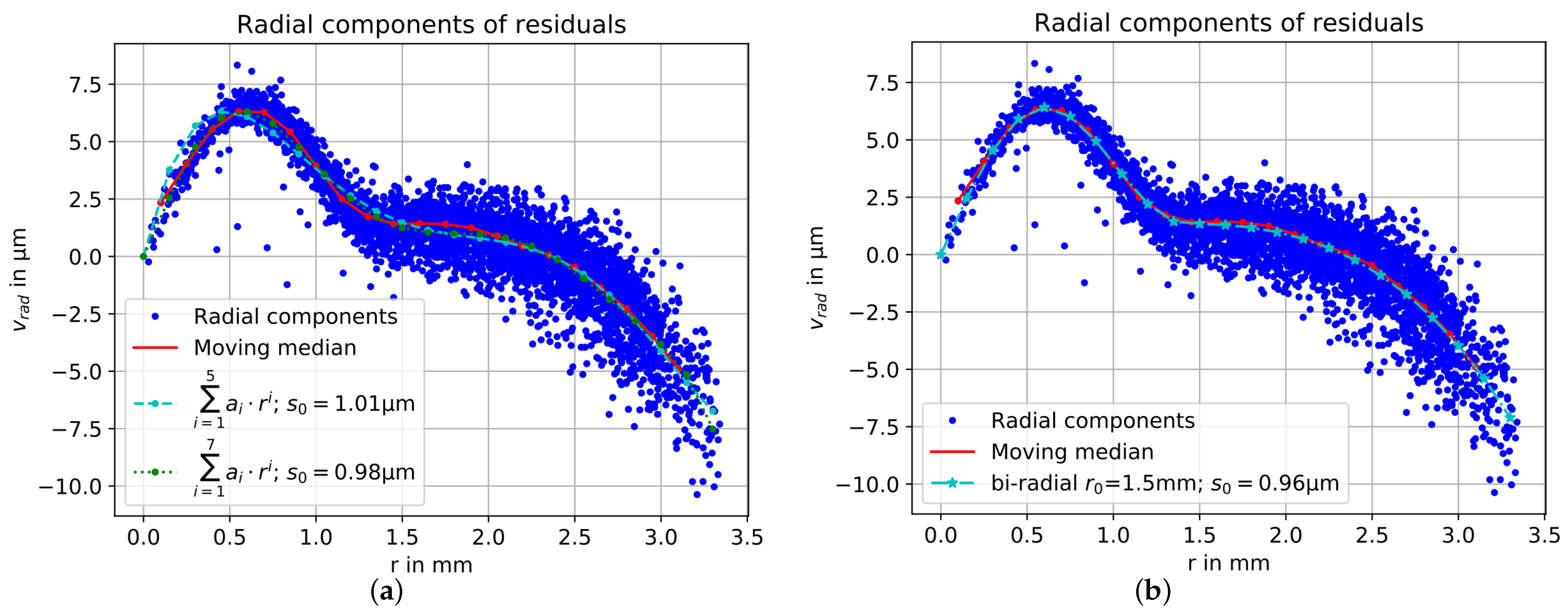
The extended polynomials are displayed in Figure 9a. With the adapted Brown model, the standard deviation of the unit weight $s_0$ (polynomial fit) can be decreased to 1.01 µm (0.65 px) and 0.98 µm (0.63 px) when using five or seven parameters, respectively.

2.3. Bi-Radial Polynomial Model

In our new approach, we combine two Brown polynomials. This approach was inspired by the residual plots shown in Figure 4 and Figure 6a. The image space is divided into two concentric radial zones with a separate set of radial distortion parameters defined and determined for each zone, i.e., a bi-radial approach. The polynomials are then applied as follows:

$$\Delta r=\left\{\begin{array}{cc}{a}_{1,0}·r+a_{1,1}·r^3+a_{1,2}·r^5+a_{1,3}·r^7\hfill & \mathrm{for}r<r_0\hfill \\ a_{2,0}·r+a_{2,1}·r^3+a_{2,2}·r^5+a_{2,3}·r^7\hfill & \mathrm{for}r>=r_0\hfill \end{array}\right.$$

(13)

Initially, the value $r_0$ was manually set to 1.5 mm. The standard deviation of the unit weight after the polynomial fit was $s_0$ = 0.96 µm (0.62 px). Figure 9b shows the fitted bi-radial function as well as the radial components as a function of r.

Both extended polynomials fit much better to the radial components than the standard Brown polynomial. This holds especially for the center region of the image, which is most relevant for tasks such as orthophoto mosaic generation. Note that the bi-radial model performs slightly better, which can also be seen in the graphs in Figure 9.

2.4. Bundle Adjustment with the Extended Radial Correction Functions

Both extended functions of Section 2.2 and Section 2.3 for the radial distortion correction were implemented in bundle adjustments. The model in [15], with addition of additional even coefficients ($O_1,O_2,O_3$) to the Brown model and hence in total using six parameters for the radial distortion description, is included in model C. Thus, the corresponding radial correction function was used:

$${\Delta r}_{extensionC}=O_1·r^2+A_1·r^3+O_2·r^4+A_2·r^5+O_3·r^6+A_3·r^7$$

(14)

Model C: Full polynomial radial distortion model

Step 1: ${\overrightarrow{X}}_c={\left(\begin{array}{ccc}{X}_c& Y_c& Z_c\end{array}\right)}^T={\mathbf{R}}^T·({\overrightarrow{X}}_w-{\overrightarrow{X}}_{projC})$

Step 2: $\left(\begin{array}{c}{x}_c\\ y_c\end{array}\right)=-\frac{c}{Z_c}·\left(\begin{array}{c}{X}_c\\ Y_c\end{array}\right)$

Step 3: $\left(\begin{array}{c}\Delta x\\ \Delta y\end{array}\right)=\frac{{\Delta r}_{extensionC}}{r}·\left(\begin{array}{c}{x}_c\\ y_c\end{array}\right)+\left(\begin{array}{c}{B}_1·(r^2+2·x_c^2)+2·B_2·x_c·y_c+C_1·x_c+C_2·y_c\\ B_2·(r^2+2·y_c^2)+2·B_1·x_c·y_c\end{array}\right)$

with $r=\sqrt{x_c^2+y_c^2}$ and $\Delta r$${}_{extensionC}$$=O_1·r^2+A_1·r^3+O_2·r^4+A_2·r^5+O_3·r^6+A_3·r^7$

Step 4: $\left(\begin{array}{c}{x}_i\\ y_i\end{array}\right)=\left(\begin{array}{c}{x}_p\\ y_p\end{array}\right)+\left(\begin{array}{c}{x}_c\\ y_c\end{array}\right)+\left(\begin{array}{c}\Delta x\\ \Delta y\end{array}\right)$

Model C was applied to the image data of the DJI Mavic Pro camera. Again, the object coordinates of the reference target field (obtained photogrammetically using the Panasonic Lumix DMC-GX80 camera) were kept fixed during the bundle adjustment. The computed parameters $p_i$ with their standard deviations $s_{p,i}$ and significance values are summarized in

Table 2. Interior orientation parameters of Model C, their standard deviation and significance.

Parameter	Estimated Value	Standard Deviation	Significance $|\frac{{\mathit{p}}_{\mathit{i}}}{{\mathit{s}}_{\mathit{p},\mathit{i}}}|$
c	4.6894 mm	0.0031 mm	1500
$x_p$	−0.03608 mm	0.00029 mm	120
$y_p$	0.00121 mm	0.00021 mm	5.8
$O_1$	−0.0278 mm${}^{-1}$	0.0028 mm${}^{-1}$	9.9
$A_1$	0.1061 mm${}^{-2}$	0.0045 mm${}^{-2}$	24
$O_2$	−0.1074 mm${}^{-3}$	0.0036 mm${}^{-3}$	30
$A_2$	0.0499 mm${}^{-4}$	0.0015 mm${}^{-4}$	33
$O_3$	−0.01110 mm${}^{-5}$	0.00033 mm${}^{-5}$	34
$A_3$	0.000960 mm${}^{-6}$	0.000029 mm${}^{-6}$	34
$B_1$	0.0000739 mm${}^{{-}^1}$	0.0000049 mm${}^{-1}$	15
$B_2$	−0.0000457 mm${}^{-1}$	0.0000035 mm${}^{-1}$	13
$C_1$	0.000054	0.000011	5.1
$C_2$	−0.0003508	0.0000099	36

.

Table 3. Correlations between the parameters of model C.

	c	$x_p$	$y_p$	$O_1$	$A_1$	$O_2$	$A_2$	$O_3$	$A_3$	$B_1$	$B_2$	$C_1$	$C_2$
c	1
$x_p$	0.003	1
$y_p$	−0.02	0.042	1
$O_1$	−0.971	0.011	−0.002	1
$A_1$	0.93	−0.014	0.006	−0.988	1
$O_2$	−0.88	0.016	−0.009	0.959	−0.991	1
$A_2$	0.828	−0.018	0.012	−0.923	0.97	−0.994	1
$O_3$	−0.778	0.018	−0.014	0.883	−0.943	0.978	−0.995	1
$A_3$	0.73	−0.019	0.016	−0.843	0.912	−0.957	0.983	−0.996	1
$B_1$	−0.025	0.888	0.048	0.024	−0.026	0.026	−0.025	0.024	−0.023	1
$B_2$	0.009	0.053	0.722	−0.008	0.008	−0.007	0.006	−0.004	0.003	0.045	1
$C_1$	0.019	0.029	0.076	0.008	−0.012	0.016	−0.019	0.022	−0.024	0.02	0.084	1
$C_2$	0.027	−0.052	−0.056	−0.026	0.025	−0.024	0.023	−0.021	0.02	−0.017	0	0.008	1

shows the correlations between the parameters of model C. The radial distortion parameters ($A_1$, $A_2$, $A_3$, $O_1$, $O_2$, $O_3$) reveal high correlation values between each other, partly almost 100%. High correlations between radial distortion parameters are a typical phenomenon, even for model B.

In model D, the second extension option, i.e., the bi-radial radial distortion correction, was integrated (see Equation (15)).

$${\Delta r}_{extensionD}=\left\{\begin{array}{cc}{A}_{1,0}·r+A_{1,1}·r^3+A_{1,2}·r^5+A_{1,3}·r^7\hfill & \mathrm{for}r<r_0\hfill \\ A_{2,1}·r^3+A_{2,2}·r^5+A_{2,3}·r^7\hfill & \mathrm{otherwise}\hfill \end{array}\right.$$

(15)

Model D: Bi-radial distortion model

Step 1: ${\overrightarrow{X}}_c={\left(\begin{array}{ccc}{X}_c& Y_c& Z_c\end{array}\right)}^T={\mathbf{R}}^T·({\overrightarrow{X}}_w-{\overrightarrow{X}}_{projC})$

Step 2: $\left(\begin{array}{c}{x}_c\\ y_c\end{array}\right)=-\frac{c}{Z_c}·\left(\begin{array}{c}{X}_c\\ Y_c\end{array}\right)$

Step 3: $\left(\begin{array}{c}\Delta x\\ \Delta y\end{array}\right)=\frac{{\Delta r}_{extensionD}}{r}·\left(\begin{array}{c}{x}_c\\ y_c\end{array}\right)+\left(\begin{array}{c}{B}_1·(r^2+2·x_c^2)+2·B_2·x_c·y_c+C_1·x_c+C_2·y_c\\ B_2·(r^2+2·y_c^2)+2·B_1·x_c·y_c\end{array}\right)$

with $r=\sqrt{x_c^2+y_c^2}$ and $\Delta r$${}_{extensionD}$$=\left\{\begin{array}{cc}{A}_{1,0}·r+A_{1,1}·r^3+A_{1,2}·r^5+A_{1,3}·r^7\hfill & \mathrm{for}r<r_0\hfill \\ A_{2,1}·r^3+A_{2,2}·r^5+A_{2,3}·r^7\hfill & \mathrm{otherwise}\hfill \end{array}\right.$

Step 4: $\left(\begin{array}{c}{x}_i\\ y_i\end{array}\right)=\left(\begin{array}{c}{x}_p\\ y_p\end{array}\right)+\left(\begin{array}{c}{x}_c\\ y_c\end{array}\right)+\left(\begin{array}{c}\Delta x\\ \Delta y\end{array}\right)$

The estimated parameters of the interior orientation with their standard deviations and significance values are summarized in

Table 4. Interior orientation parameters of Model D, their standard deviation and significance.

Parameter	Estimated Value	Standard Deviation	Significance $|\frac{\mathit{p}}{{\mathit{s}}_{\mathit{p}}}|$
c	4.75027 mm	0.00055 mm	8600
$x_p$	−0.03619 mm	0.00028 mm	130
$y_p$	0.00125 mm	0.00020 mm	6.2
$A_{1,0}$	−0.01530 mm${}^{-1}$	0.00015 mm${}^{-1}$	99
$A_{1,1}$	0.01959 mm${}^{-2}$	0.00037 mm${}^{-2}$	53
$A_{1,2}$	−0.00776 mm${}^{-3}$	0.00031 mm${}^{-3}$	25
$A_{1,3}$	0.000978 mm${}^{-4}$	0.000079 mm${}^{-4}$	12
$A_{2,1}$	0.000344 mm${}^{-5}$	0.000045 mm${}^{-5}$	7.7
$A_{2,2}$	−0.0000056 mm${}^{-6}$	0.0000074 mm${}^{-6}$	0.76
$A_{2,3}$	0.00000101 mm${}^{-6}$	0.00000038 mm${}^{-6}$	2.6
$B_1$	0.0000702 mm${}^{-1}$	0.0000046 mm${}^{-1}$	15
$B_2$	−0.0000441 mm${}^{-1}$	0.0000032 mm${}^{-1}$	14
$C_1$	0.000049	0.000010	4.9
$C_2$	−0.0003453	0.0000094	37
$r_0$	1.5 mm

. Note that the standard deviation of the camera constant is ca. five times smaller in model D due to a more relaxed correlation situation.

Table 5. Correlations between the parameters of model D.

	c	$x_p$	$y_p$	$A_{1,0}$	$A_{1,1}$	$A_{1,2}$	$A_{1,3}$	$A_{2,1}$	$A_{2,2}$	$A_{2,3}$	$B_1$	$B_2$	$C_1$	$C_2$
c	1
$x_p$	0.062	1
$y_p$	−0.102	0.041	1
$A_{1,0}$	−0.368	0.005	−0.005	1
$A_{1,1}$	−0.013	−0.006	0.011	−0.795	1
$A_{1,2}$	0.008	0.002	−0.008	0.732	−0.98	1
$A_{1,3}$	−0.004	−0.001	0.006	−0.679	0.944	−0.99	1
$A_{2,1}$	−0.692	−0.008	0.013	0.523	0.011	−0.008	0.005	1
$A_{2,2}$	0.667	0.007	−0.019	−0.508	−0.011	0.008	−0.005	−0.991	1
$A_{2,3}$	−0.638	−0.006	0.022	0.489	0.01	−0.007	0.004	0.969	−0.993	1
$B_1$	−0.02	0.888	0.047	0.014	−0.009	0.005	−0.002	0.003	−0.003	0.003	1
$B_2$	0.012	0.052	0.718	−0.008	−0.001	0.002	−0.003	−0.022	0.018	−0.016	0.044	1
$C_1$	0.148	0.028	0.076	−0.011	−0.001	−0.001	0.001	−0.02	−0.004	0.019	0.019	0.084	1
$C_2$	0.008	−0.054	−0.058	−0.001	−0.004	0.005	−0.007	−0.006	0.005	−0.004	−0.019	−0.002	0.008	1

shows the correlations between the parameters of model D. The parameter groups for the radial distortion correction (group 1: $A_{1,0}$, $A_{1,1}$, $A_{1,2}$, $A_{1,3}$ and group 2: $A_{2,1}$, $A_{2,2}$, $A_{2,3}$) reveal high correlation values between each other within the groups, sometimes almost 100%. However, the correlations between groups are close to zero.

Table 6. Standard deviation of the unit weight after the bundle adjustment with fixed object coordinates and considering different models describing lens distortions.

Model	${\mathit{s}}_0$ after Bundle Adjustment
Model A (pure pinhole model)	0.00211 mm $\widehat{=}$ 1.37 px
Model B (standard distortion model—Brown)	0.00098 mm $\widehat{=}$ 0.64 px
Model C according to [15]	0.00057 mm $\widehat{=}$ 0.37 px
Model D (bi-radial $r_0=1.5$ mm—our method)	0.00054 mm $\widehat{=}$ 0.35 px

depicts the standard deviations of the unit weights $s_0$ of the bundle adjustments of the different models applied to the data of the DJI Mavic Pro camera to enable a first assessment of differences between different approaches. It already becomes obvious that models C and D reveal a similar performance and that they seem to be significantly better than Model B. A further accuracy analysis is shown in Section 2.7.

2.5. Systematic Effects in the Residual Errors of the Extended Distortion Models

Residual plots were computed to give a visual impression of potential remaining systematic residual errors (Figure 10 for model C and Figure 11 for model D, i.e., bi-radial). Both plots show randomly distributed residuals that have much smaller magnitudes compared to those in model B (see Figure 4).

Again, the residuals were decomposed into a radial and tangential part. Figure 12 shows the result for model C, whereas Figure 13 depicts the components for the bi-radial model (D). For model C, an oscillation in the radial components becomes obvious (Figure 12a). This effect could be caused by the high correlations between the radial distortion parameters of model C. The correlations between the parameter groups for radial distortion of model D are close to zero. However, this effect does not influence the standard deviation of the unit weight significantly. The components reveal the aspired non-systematic behavior for the bi-radial model D (Figure 13a).

2.6. Strategy for Automatic Zone Segmentation of the Bi-Radial Model

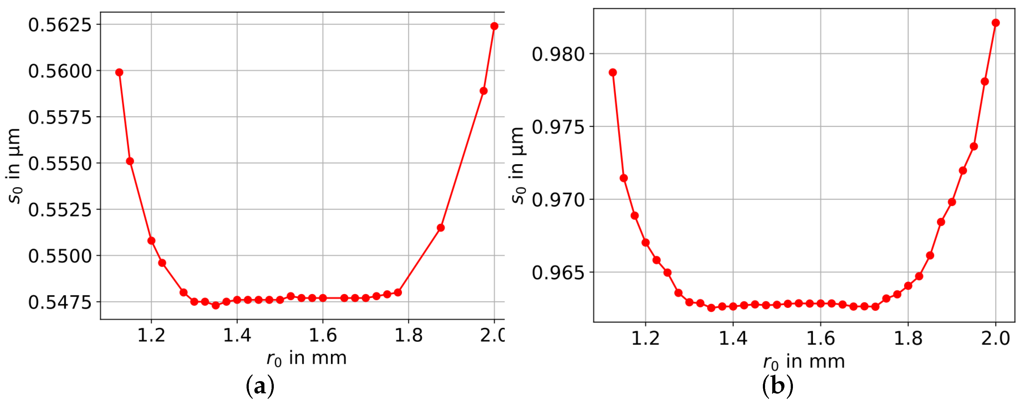
To date, the radial zone segmentation radius $r_0$ of the bi-radial model had been manually set to 1.5 mm. In general, the optimal value should be determined automatically. However, $r_0$ cannot be estimated in bundle adjustment due to its discrete nature. An obvious first approach is an iterative (brute force) computation of the bundle adjustment with different values of $r_0$, where the best $r_0$ corresponds to the lowest standard deviation of the unit weight. Accordingly, Figure 14a shows the standard deviation of the unit weight as a function of the limit value $r_0$. In the range of 1.3 mm $<r_0<$ 1.8 mm, $s_0$ does not change significantly, indicating that the selection of the segmentation value for the concentric zones is rather uncritical.

A much less computationally intensive approach is the brute force computation of the polynomial fit introduced in Section 2.1. Only one bundle adjustment using model A is performed for the polynomial analysis. Then, the radial components of the residuals are calculated (Equation (9)). Afterwards, a polynomial fit in the residual data is performed by a step-wise increase in the values of $r_0$. The standard deviation of the unit weight of the polynomial fit as a function of $r_0$ is displayed in Figure 14b. The behavior coincides with the former approach (shown in Figure 14a), and therefore the polynomial analysis is recommended.

2.7. Validation

The aim of this subsection is to evaluate the accuracy of the proposed extended models C and D. Their validation was performed by comparing the object coordinates, which were calculated in a free net adjustment (self-calibration) using images captured with the UAV camera, to the reference coordinates, which were independently obtained by a second camera with a significantly higher accuracy potential (Nikon D300 camera (from company Nikon) with a Nikkor lens with a focal length of 20 mm). The same target field as in Section 2.1 was used (Figure 5; 7 m × 3 m × 1 m), this time with four additional scale bars of superior precision included. Figure 15 shows the object points and the position of the scale bars as well as the image network geometry used for both cameras.

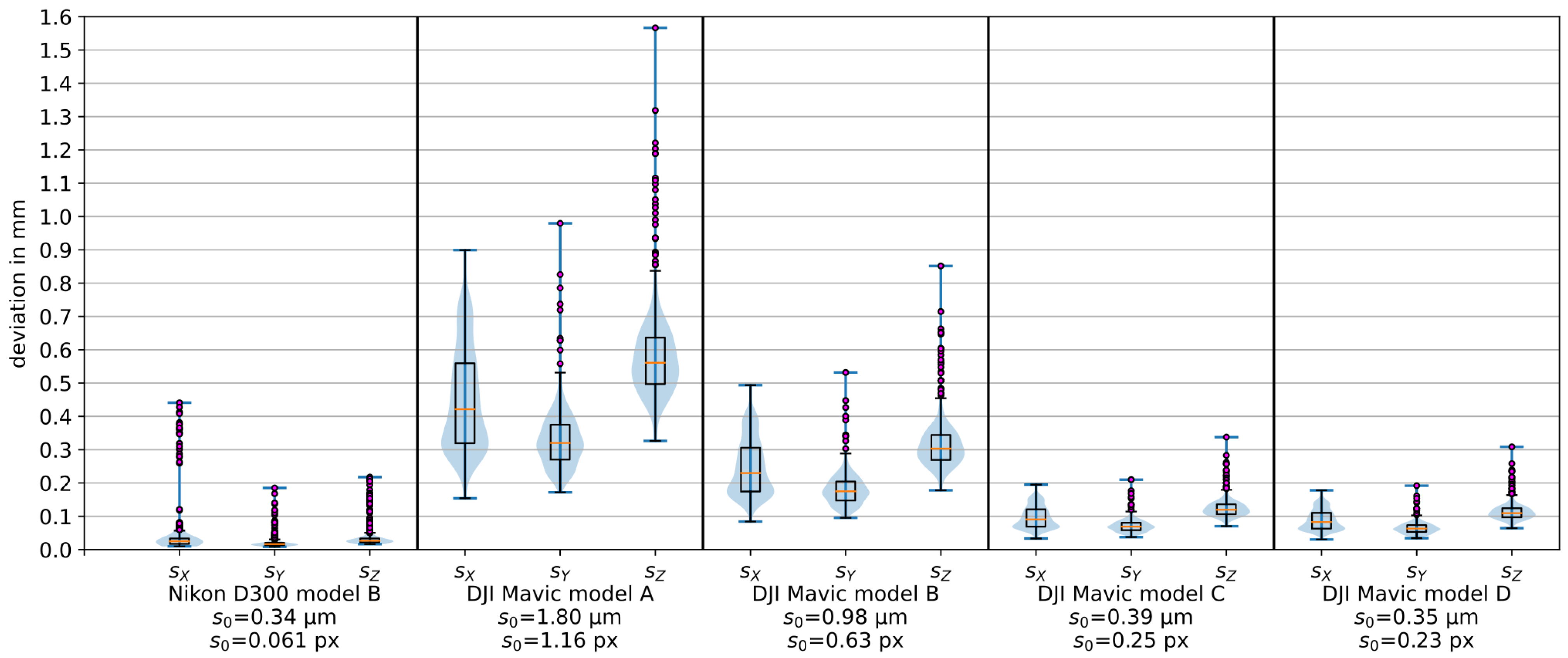
Figure 16 shows the combined violin plots (including extreme values, blue) and box plots (including outliers in magenta) of the standard deviations ($s_X$, $s_Y$, $s_Z$) of the object point coordinates from the bundle adjustment. The standard deviations of the unit weights are also listed below the plots. The Nikon D300 camera revealed the smallest values for the standard deviations (left side of Figure 16). The standard deviations of the DJI Mavic Pro camera—computed with the different models B, C and D - highlight that the errors could be reduced using models C and D. The median of $s_Z$ was reduced by two thirds in the case of model D when compared to model B. Models C and D (bi-radial) showed a similar behavior, with model D indicating slightly better values. However, both models still exhibited higher standard deviations compared to the values obtained with the Nikon camera data (using model B).

In order to evaluate the accuracy of the different models, the object coordinate sets obtained from the image bundles of both cameras (DJI Mavic Pro and Nikon D300) were compared, with the latter camera providing the reference coordinates. Therefore, the parameters of a least-squares rigid transformation were computed to align the coordinates to the reference. The rigid body transform was chosen because the bundle adjustment was performed with scale bars so that the scale is comparable between the coordinate sets. The distribution of the residual vectors is visualized on the left side of Figure 17. The estimation of the parameters was performed between the data sets of the Nikon D300 using model B and the DJI Mavic Pro using different models (i.e., model B in Figure 17a, model C in Figure 17b, model D in Figure 17c). Model C and model D show significantly smaller residual vectors than model B. Differences between model C and D are hardly noticeable. The standard deviations of the unit weights of the parameter determination of the rigid body transformation were 0.39 mm for the first case (DJI model B), 0.23 mm for the second (DJI model C), and 0.24 mm the third case (DJI model D).

Residual systematics are still visible in Figure 17 and deviations, especially of the points in the foreground, are noticeable. Due to their smaller number, these foreground points have a smaller effect on the transformation parameter computation than the many more points on the wall in the background. This circumstance may lead to higher residuals.

Figure 17 also shows the combined violin and box plots for the residual vector lengths of the rigid body transform using the different models for the DJI Mavic Pro camera. The median residual vector length is 0.62 mm for the first case (standard Brown model B) and the maximum amounts to 2.1 mm. For models C and D, the median residual vector length is 0.35 mm and the maximum deviations are 1.1 mm. These (standard) deviations are considered as accuracy values.

3. Discussion

Based on the results presented, the following conclusions were drawn:

• In this study, we could demonstrate that the estimation of a bi-radial distortion model can decrease the errors during bundle adjustment when using low-cost UAV cameras that might be difficult to model with standard, physics-based models such as the Brown model. The unusual systematic errors of the DJI Mavic Pro camera could be reduced using the proposed bi-radial model (model D) as well as model C (extended polynomial of radial distortion). The standard deviations of the unit weights of the bundle adjustment could be significantly reduced (60% for model C and 64% for model D). The improvement was also recognizable visually in the residual vector plots. The improvement was most evident in the center of the images.
• In model C, some residual systematics still remained (Figure 12a), which were no more visible in our proposed model D (Figure 13a).
• In contrast to model C, a segmentation zone radius $r_0$ has to be determined for our proposed model D. Our experiments revealed that there was a range, between 1.3 mm and 1.8 mm, in which the results did not change significantly. Furthermore, an automatic determination method is possible (as shown in Section 2.6). The additional step of the determination of $r_0$ requires a higher computing effort compared to model C.
• For the accuracy evaluation, the object coordinates computed via free bundle adjustment of the DJI Mavic Pro camera with the different models were compared to the reference coordinates obtained by a well-known camera. The residuals of a rigid body transformation were analyzed, where the standard deviation of the unit weight of the transformation was reduced by 40% using models C and D compared to the standard Brown model (model B). Model C and model D showed similar residuals and the differences were hardly noticeable.
• Future work could concentrate on a constraint in which the polynomials of the bi-radial model fit together at the transition point between both zones concerning function value and the derivative similar to spline constraints.

4. Conclusions

Popular low-cost UAV-based cameras such as the very widespread DJI Mavic Pro camera often show unusual lens distortion patterns, which cannot be handled well by standard camera modeling and calibration approaches. We introduce a novel bi-radial lens distortion model consisting of separate polynomials for two concentric image zones. While standard models show clear systematic effects in residual plots after bundle adjustment, the new model provides significantly better precision values and leaves no systematic effects in the residual plot, with the most evident improvement at the image center. The segmentation of the image space into the two zones can be performed automatically and this turned out to be rather uncritical. The model may also be useful for modeling mobile phone imaging devices and other similar low-cost cameras. It may also be easily extended to a segmentation of the image into more than two concentric zones.

References

1. Schmid, H.H. Eine allgemeine analytische Lösung für die Aufgabe der Photogrammetrie. Bildmess. Luftbildwes. 1958, 4/58, 103–113. [Google Scholar]
2. von Seidel, P.L. Ueber die Theorie der Fehler, mit welchen die durch optische Instrumente gesehenen Bilder, behaftet sind, und über die mathematischen Bedingungen ihrer Aufhebung. In Abhandlungen der Naturwissenschaftlich-Technischen Commission bei der Königl; Bayerischen Akademie der Wissenschaften in München: Munich, Germany, 1857; Volume 1, Chapter 10; pp. 227–267. [Google Scholar]
3. Brown, D.C. Close-Range Camera Calibration. Photogramm. Eng. 1971, 37, 855–866. [Google Scholar]
4. Conrady, A.E. Decentred Lens-Systems. Mon. Not. R. Astron. Soc. 1919, 79, 384–390. [Google Scholar] [CrossRef]
5. Brown, D.C. Decentering distortion of lenses. Photogramm. Eng. 1966, 32, 444–462. [Google Scholar]
6. Luhmann, T.; Robson, S.; Kyle, S.; Boehm, J. Close-Range Photogrammetry and 3D Imaging; De Gruyter: Berlin, Germany; Boston, MA, USA, 2020. [Google Scholar] [CrossRef]
7. El-Hakim, S.F. Real-Time Image Metrology with CCD Cameras. Photogramm. Eng. Remote Sens. 1986, 52, 1757–1766. [Google Scholar]
8. Luhmann, T.; Fraser, C.; Maas, H.G. Sensor modelling and camera calibration for close-range photogrammetry. Isprs J. Photogramm. Remote Sens. 2016, 115, 37–46. [Google Scholar] [CrossRef]
9. Ebner, H. Self calibrating block adjustment. In Proceedings of the XIII ISP Congress, Helsinki, Finland, 11–23 July 1976; pp. 540–558. [Google Scholar]
10. Grün, A. Experiences with the self-calibrating bundle adjustment. In Proceedings of the ACSM-ASP Convention, Washington, DC, USA, 3 March 1978. [Google Scholar]
11. Abraham, S.; Förstner, W. Zur automatischen Modellwahl bei der Kalibrierung von CCD-Kameras. In Mustererkennung 1997; Paulus, E., Wahl, F.M., Eds.; Springer: Berlin/Heidelberg, Germany, 1997; pp. 147–155. [Google Scholar] [CrossRef]
12. Tang, R. New mathematical self-calibration models in aerial photogrammetry. In Proceedings of the DGPF-Tagungsband, Potsdam, Germany, 14–17 March 2012; Volume 21, pp. 457–469. [Google Scholar]
13. Tang, R. A rigorous and flexible calibration method for digital airborne camera systems. Int. Arch. Photogramm. Remote Sens. Spatial Inf. Sci. 2012, 39, 153–158. [Google Scholar] [CrossRef]
14. Richter, K.; Mader, D.; Seidl, K.; Maas, H.G. Development of a geometric model for an all-reflective camera system. ISPRS J. Photogramm. Remote Sens. 2013, 86, 41–51. [Google Scholar] [CrossRef]
15. Hastedt, H.; Luhmann, T.; Przybilla, H.J.; Rofallski, R. Evaluation of interior orientation modelling for cameras with aspheric lenses and image pre-processing with special emphasis to SFM reconstruction. Int. Arch. Photogramm. Remote Sens. Spat. 2021, 43, 17–24. [Google Scholar] [CrossRef]
16. Reznicek, J.; Luhmann, T. Finite-Element Approach to Camera Modelling and Calibration. PFG J. Photogramm. Remote Sens. Geoinf. Sci. 2019, 87, 1–17. [Google Scholar] [CrossRef]
17. Detchev, I.; Lichti, D. Calibrating a lens with a local distortion model. Int. Arch. Photogramm. Remote Sens. Spat. 2020, 43, 765–769. [Google Scholar] [CrossRef]
18. Eltner, A.; Karrasch, P.; Stoecker, C.; Klingbeil, L.; Hoffmeister, D.; Kaiser, A.; Rovere, A. UAVs in Environmental Sciences—Methods and Applications; WBG Academic: Darmstadt, Germany, 2022. [Google Scholar] [CrossRef]
19. Eltner, A.; Bertalan, L.; Grundmann, J.; Perks, M.T.; Lotsari, E. Hydro-morphological mapping of river reaches using videos captured with UAS. Earth Surf. Process. Landf. 2021, 46, 2773–2787. [Google Scholar] [CrossRef]
20. James, M.R.; Antoniazza, G.; Robson, S.; Lane, S.N. Mitigating systematic error in topographic models for geomorphic change detection: Accuracy, precision and considerations beyond off-nadir imagery. Earth Surf. Process. Landf. 2020, 45, 2251–2271. [Google Scholar] [CrossRef]
Figure 1. Pinhole model. The corresponding X axis is colored red, Y in green and Z in blue. The ray from the object point into the image is depicted in magenta. The principal point is the perpendicular foot of the projection center onto the image.
Remotesensing 15 05283 g001
Figure 2. Upper part: Correction vectors for symmetric radial lens distortion for different parameter examples of a virtual camera. Lower part: Corresponding radial corrections as a function of the image radius.
Remotesensing 15 05283 g002
Figure 3. Correction vectors for decentering lens distortion of a virtual camera for different parameter examples.
Remotesensing 15 05283 g003
Figure 4. Residual plot after free net bundle adjustment using model B.
Remotesensing 15 05283 g004
Figure 5. (a) Reference target field used for bundle adjustments. (b) Orientation of the images of the Panasonic Lumix DMC-GX80 camera and locations of the object points. The schematic illustration was created with the software package AICON 3D Studio (version 12.50.03).
Remotesensing 15 05283 g005
Figure 6. (a) Residual plot after bundle adjustment using model A (i.e., pure pinhole model) with fixed object coordinates. (b) Decomposition of the residual vector into radial and tangential components.
Remotesensing 15 05283 g006
Figure 7. (a) Radial components of the residuals plotted against the image radius. (b) Tangential components of the residuals plotted against the image radius. (c) Radial components plotted against the azimuth of the image point. (d) Tangential components plotted against the azimuth of the image point. For all subplots, the moving median is shown in red.
Remotesensing 15 05283 g007
Figure 8. Radial components and fitted Brown polynomials with standard deviations of the unit weight of the polynomial fit.
Remotesensing 15 05283 g008
Figure 9. (a) Radial components and fitted polynomials with Equations (11) and (12). (b) Radial components and fitted bi-radial polynomials of Equation (13). Both with standard deviations of the unit weight of the polynomial fit.
Remotesensing 15 05283 g009
Figure 10. Residual plot after bundle adjustment with fixed object coordinates using model C.
Remotesensing 15 05283 g010
Figure 11. Residual plot after bundle adjustment with fixed object coordinates using model D.
Remotesensing 15 05283 g011
Figure 12. Residuals after bundle adjustment using model C. (a) Radial components versus image radius. (b) Tangential components versus image radius. (c) Radial components versus the azimuth of the image point. (d) Tangential components versus the azimuth of the image point. For all subplots, the moving median is shown in red.
Remotesensing 15 05283 g012
Figure 13. Residuals after bundle adjustment using model D: (a) Radial components versus image radius. (b) Tangential components versus image radius. (c) Radial components versus the azimuth of the image point. (d) Tangential components versus the azimuth of the image point. For all subplots, the moving median is shown in red.
Remotesensing 15 05283 g013
Figure 14. (a) Standard deviation of the unit weight s 0 of the bundle adjustment as a function of r 0 . (b) Standard deviation of the unit weight s 0 of the polynomial fit as a function of r 0 .
Remotesensing 15 05283 g014
Figure 15. Object points and scale bars as well as the image orientations (illustration created with AICON 3D Studio (version 12.50.03)).
Remotesensing 15 05283 g015
Figure 16. Combined violin and box plots of the object coordinates’ standard deviations computed in the bundle adjustment and corresponding standard deviation of the unit weight ( s 0 ) in mm and in px.
Remotesensing 15 05283 g016
Figure 17. Residuals (left side, scale factor 300) and combined violin and box plots (right side) for the residuals’ lengths of the rigid body transformation between: (a) DJI Mavic Pro camera (model B) and Nikon D300 camera (model B), (b) DJI Mavic Pro camera (model C) and Nikon D300 camera (model B), (c) DJI Mavic Pro camera (model D) and Nikon D300 camera (model B).
Remotesensing 15 05283 g017