Abstract
The interferometric imaging radar altimeter (InIRA), mounted on the Tiangong-2 space laboratory, utilizes a small incidence and a short interferometric baseline to achieve altimetry for wide swathes of ocean surface topography and inland water surface elevation. To obtain a high-precision digital elevation model (DEM), calibration of the interferometric system parameters is necessary. Because InIRA utilizes the small-incidence interference system design, serious coupling occurs between the interferometric parameters. Commonly used interferometric calibration methods tend to fall into the local optimal solution for InIRA. Because evolutionary algorithms have a stronger robustness and global search ability, they are better suited to handling the solution space structure under the coupling of complex interferometric parameters. This article establishes an interferometric calibration optimization model for InIRA by utilizing the relative flatness of the lake surface as an inequality constraint. Furthermore, an adaptive penalty coefficient constraint evolutionary algorithm is designed to solve the model. The proposed method was tested on actual InIRA data, and the results indicate that it efficiently adjusts interferometric parameters, enhancing the precision of measurements for Qinghai Lake elevation.
1. Introduction
A radar altimeter is an active remote sensing system that measures the distance between a platform and the Earth’s surface by transmitting electromagnetic pulses to the ground, receiving reflected echoes, and calculating the time delay between the transmitted and received signals [1]. Spaceborne radar altimeters are primarily used for ocean observation. They obtain the sea surface echo waveform and precisely track the half-power point of the echo waveform to determine the accurate distance from the satellite platform to the mean sea level. The height of the mean sea level can then be determined using precise orbit determination data from the satellite. Over the past thirty years, numerous altimeter satellites have been launched globally, with the accuracy of data observation increasing from meter to centimeter levels [1]. Satellites such as Seasat [2], Geosat [3], Jason-3 [4], and Sentinel-3 [5] have been launched in the past five decades for oceanography purposes.
Although traditional ocean altimeters have reached centimeter-level measurement accuracy, they are limited by narrow swath and low spatial resolution. Altimeters that use interferometry technology can achieve high spatial resolution and wide swath when measuring the sea level, which is crucial for observing mesoscale and submesoscale ocean phenomena. The Surface Water and Ocean Topography (SWOT) mission [6,7], launched in December 2022, will provide important observational data for precise measurements of global surface water and ocean surfaces. The KaRIN interferometric altimeter is an important payload on the SWOT satellite. It is a Ka-band radar interferometer, including two 5 m-long radar antennas on the left and right. The observation width of SWOT can reach 120 km, and it can obtain two-dimensional height information at the same time, which is beyond the reach of traditional altimeters.
Calibrating the interferometric system parameters with external calibration methods is necessary to enhance the accuracy of the elevation data. Several research efforts have focused on InSAR calibration [8]. The primary aim of these studies is to analyze different error parameters and develop an error model that impacts elevation data accuracy. This error model is subsequently applied to correct the digital elevation model (DEM) product and enhance DEM data accuracy. The baseline is a crucial interferometric calibration parameter among other interferometric system parameters. It affects not only the removal of the earth’s flat phase but also the conversion between terrain phase and elevation, as well as the precision of surface deformation measurements. Various methods have been developed to enhance the accuracy of the baseline and DEM products. These methods include the traditional orbit estimation method [9,10], high-precision ground control point (GCP) method [11,12,13,14], and the fringe change rate estimation method [15]. Selecting an appropriate method to estimate or correct the baseline is essential to guarantee precise elevation data.
The GCP method is the most accurate method for estimating baselines, albeit it is also the most complicated in terms of calculation and implementation. This method necessitates precise ground elevation data and the resolution of equations that combine the baseline and control points. In contrast to other baseline estimation algorithms, the GCP method offers superior baseline estimation accuracy and can fulfill the demands of high-precision terrain mapping. Nevertheless, deploying ground control points in the survey area must satisfy specific prerequisites, and there is no assurance that appropriate control points fulfilling the requirements exist globally. Therefore, investigating interferometric parameter calibration in regions without ground control points is essential. Some researchers have examined natural landscapes as a means of calibrating InSAR system parameters without ground control points [16], while others have used flat inland regions to calibrate airborne InSAR interferometric parameters [17]. However, this method must be implemented when the parameter error range is small; otherwise, it results in a consistent elevation error.
The primary method of calibrating interferometric parameters using ground control points involves solving the interferometric parameters through a sensitivity matrix [8] and optimization equation [18]. The sensitivity matrix method separates the influence of interferometric parameters on the elevation error, expressing the error caused by each interferometric parameter error source linearly. The interferometric parameter sensitivity matrix is then established, and the interferometric parameter error is solved using linear least squares. However, the approximating linearization errors between the interferometric parameters and the elevation error can result in certain errors in the results. Additionally, the sensitivity matrix’s condition number can be too large, making the inversion of the matrix unstable. Another commonly used optimization method minimizes the objective equation using traditional optimization algorithms, reducing the elevation difference between the generated elevation and the ground control point, ensuring the interferometric parameters meet the required equation’s requirements. And traditional optimization algorithms often struggle with multidimensional searches due to the strong coupling between interferometric parameters during the solution, resulting in local optimal solution.
In order to obtain interferometric parameters with a high accuracy and improve the optimization capability of the interferometric calibration algorithm, this paper proposes a novel interferometric calibration method without ground control points. This method first establishes optimization equations based on the relative flatness of the terrain and solves them using the intelligent evolutionary algorithm. Then, an adaptive penalty coefficient is introduced to dynamically adjust the optimization range of the algorithm, which adapts its size during the search process. In experiments, the proposed algorithm is validated using InIRA data. Compared with several commonly used algorithms, it demonstrates advantages in terms of accuracy.
2. InIRA Three-Dimensional Reconstruction and Elevation Error Analysis
2.1. InIRA Three-Dimensional Reconstruction Model
The InIRA, developed by the National Space Science Center, Chinese Academy of Sciences, is a wide swath near-nadir incidence cross-orbit InSAR borne on the Tiangong-2 space laboratory. The baseline length between its two Ku-band antennas is 2.3 m. To improve surveying accuracy and increase the surveying width, the InIRA incidence is designed to obtain a swath with a width of over 40 km [6]. Compared with an altimeter, InIRA can obtain a larger swath width, and compared with synthetic aperture radar (SAR) and interferometric SAR, InIRA has higher resolution. At the near-nadir incidence of InIRA, the water surface echo is dominated by specular reflection energy, making the data acquired by InIRA remarkable due to the near-nadir incidence and large incidence variation range. Traditional synthetic aperture radars with large incidences usually show low echo and signal-to-noise ratio (SNR) in water areas, appearing as dark areas in radar images. However, InIRA data present a higher SNR and coherence in the water area due to the small incidence, allowing the radar to receive reflected water surface echoes. And dual antennas are used to obtain highly coherent sea surface echoes for surveying and mapping.
The basic principle of the three-dimensional reconstruction model of InIRA is to obtain the three-dimensional coordinates of the ground target point by combining the distance equation, Doppler equation and interferometric phase equation. Figure 1 shows the geometric relationship of InIRA measurement in the geocentric coordinate system [19], where , is the position vector of the master and slave antenna phase center, , represents the position vector of the main and auxiliary antenna phase center to the ground point, is the ground target point position vector and is the baseline vector. In the triangle composed of the target point , the origin of the geocentric space coordinate system and the phase center of the main antenna, the vector expression of the target point in the geocentric space rectangular coordinate system can be obtained. The three-dimensional reconstruction model is composed of the distance Equation (1), radar Doppler Equation (2) and interferometric phase Equation (3):
where is the distance from the target point to the phase center of the main antenna; is the distance from the auxiliary antenna to the target point; is the satellite velocity vector; is the Doppler center frequency; is the radar wavelength; is the absolute interferometric phase; is the wrapped phase; k is the integer cycle number of the interferometric phase; Q is the antenna mode and 2 and 1, respectively, represent the repeated orbit interferometric mode and the double antenna interferometric mode.
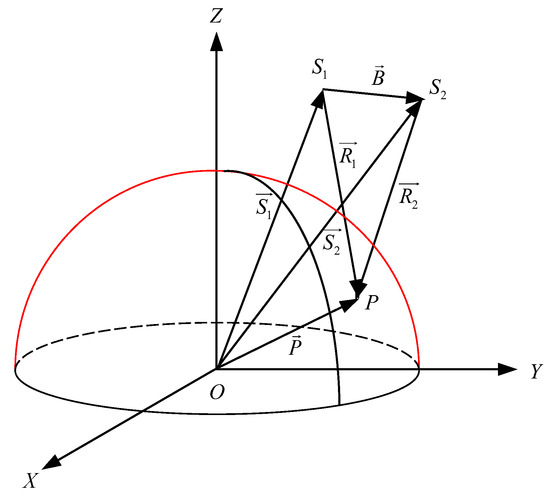
Figure 1.
InIRA topographic mapping geometric relationship.
To obtain an analytical solution to the above equation and analyze the interferometric sensitivity of elevation to various parameters while minimizing the approximation error, the paper introduces a moving coordinate system with the phase center of the main antenna serving as the origin. The unit view vector is then orthogonally projected onto this coordinate system. Subsequently, the paper achieves the transformation of the unit view vector from the moving coordinate system to the imaging coordinate system through coordinate transformation, facilitating terrain reconstruction. Based on the InIRA geometric relationship, the target point’s coordinates are expressed as follows:
where represents the unit vector of the view vector in the direction of v axis, p axis and q axis; is the conversion matrix from the view vector in the VPQ coordinate system to the Cartesian coordinate system in the geocentric space. The VPQ coordinate system takes the phase center of the main antenna as the origin of the coordinates, the direction of the velocity vector is the v axis, the cross product direction of the velocity and the baseline is the q axis and the v axis, p axis and q axis satisfy the right-handed coordinate system relationship. The visual vector decomposition method converts the visual vector from the moving coordinate system to the geocentric space rectangular coordinate system, so as to obtain the three-dimensional position information of the target point:
where is the component of the baseline in the direction of velocity; is the component of the baseline perpendicular to the direction of velocity. In InIRA, the baseline is perpendicular to the velocity direction; that is, , and the squint angle is 0; that is, , at this angle, Equation (5) degenerates into a common radar side-looking equation.
2.2. InIRA Elevation Error Analysis
The baseline is an important parameter in the InIRA system. The length and direction of the baseline vector directly affect many factors such as image coherence, altimetry sensitivity, and altimetry error transfer coefficient. The baseline vector error is also one of the most important error sources affecting the measurement accuracy. Refer to the elevation error analysis method of TanDEM-X [20]; the baseline is decomposed into a vertical baseline perpendicular to the line of sight and a parallel baseline along the line of sight. The effects of , and on InIRA elevation error are analyzed below.
InIRA is a spaceborne dual-antenna interferometric system. The main antenna transmits, and the two antennas receive simultaneously. The relationship between the elevation of the ground point and the phase after removing the ground effect is:
where is the absolute interferometric phase after phase unwrapping, and is the interferometric system ambiguity height, defined as:
where is the incidence, if there is a baseline error in the system, then the introduced altimetry error is:
Assuming that the terrain height is 3000 m, when , , the vertical baseline error mm will cause an elevation error of 1.3 m, and the error changes slowly with the increase in incidence in the range direction.
is the main error source of the interferometric system. The baseline error along the line of sight directly affects the interferometric slant range difference. Therefore, and are coupled with each other during the calibration process. The elevation error caused by the combination can be expressed as:
Because the ambiguity height changes with the range direction, and will cause the ground elevation to change along the range direction, which will cause the distance slope. If the distance length is s, the slope is:
From the above analysis, it can be concluded that the conventional space-borne InSAR elevation error is manifested as a tilt error in the range direction, which is caused by the parallel baseline error and the interferometric phase error, and the relationship between the two is coupled. Since InIRA is different from traditional long-baseline and large-incidence spaceborne interferometric systems, the error of InIRA’s vertical baseline will also have a greater impact on the elevation.
In order to analyze and determine the actual influence of baseline vector and interferometric phase on elevation error, we use the system parameters of a scene InIRA image to analyze the sensitivity of interferometric parameters to elevation based on the elevation reconstruction model. Specifically, we introduce linear errors to the baseline length, baseline inclination, and interferometric phase at the image’s center point while keeping other interferometric parameters constant. The resulting elevation error is displayed in Figure 2.
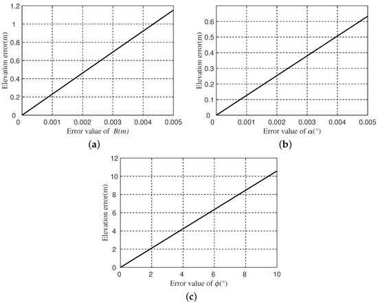
Figure 2.
The sensitivity of interferometric parameters errors to elevation. The influence of the interferometric parameter errors on the elevation at the center of the image shown as an approximately linear trend. Such a linear relationship exists in the entire range direction. (a) The influence of baseline length error on elevation; (b) the influence of baseline inclination error on elevation; (c) the influence of interferometric phase error on elevation.
Figure 2 reveals that the influence of baseline length B, baseline inclination and absolute interferometric phase on elevation is roughly linear. This is due to InIRA’s smaller incidence, which leads to a linearly coupled error contribution to the elevation, making it challenging to achieve parameter correction by separating the impact of each parameter on elevation. When conventional optimization methods are used to search for a multi-dimensional solution space, coupled interferometric parameters increase the risk of local optimal solution convergence [21,22,23]. Non-convex functions often feature multiple local optimal solutions, which impede algorithms from determining the optimal solution. Moreover, these algorithms heavily rely on gradient information or higher-order derivatives that may limit their ability to escape local optimal solutions. Hence, this paper proposes the use of a constrained optimization evolutionary algorithm in the following section to overcome this issue.
3. Optimization Calibration Method Based on Inland Water Body
3.1. InIRA Optimization Calibration Model
According to the elevation error analysis of interferometric parameters in the previous section, we take the baseline length B, baseline inclination and absolute interferometric phase as the parameters to be calibrated, which cause slope errors in the InIRA elevation, and the interferometric system quantities that do not participate in the calibration are regarded as constants; the elevation of the surface object is a nonlinear function of the system parameter variable ; and the estimation accuracy of the target point is related to the system parameter X; that is, the elevation h can be expressed as a nonlinear function of each system parameter.
The parameter error of the actual InSAR system is , and each error has a certain error range. Let , , ; that is, the solution space domain R of the system parameter error is . Assuming that the initial value of the obtained interferometric system parameter vector is and the real value is X, for the calibration based on control points, the elevation at the control points is set to , and the single point objective optimization objective function can be expressed as [18]:
where is the elevation reconstruction formula at the n th calibration point; that is, the calibration problem of the InSAR system is transformed into the problem of adjusting the error parameters to minimize the objective function, so that the elevation value after adjusting the system parameter error is the minimum distance from the elevation value at the control point. According to the interferometric coherence, different control points are weighted. Combined with the least square method to solve the model parameters, we can obtain the optimal objective function under different weights :
Different from the traditional InSAR, the near-nadir interference makes InIRA have high SNR and high correlation on the water surface. Water surfaces exhibit the characteristic of height consistency, which is an inherent property of the data. Therefore, lake elevation information can be used for interferometric calibration, utilizing the discreteness of lake elevation as a constraint term in the calibration equation, as follows:
where N is the number of calibration points on the land elevation and M is the number of calibration points on the lake elevation. In fact, due to the influence of coherence difference and random noise, the lake elevations are not completely equal, so we use the statistical information of the lake elevation to assist with calibration, and describe the constraint as the discreteness of the lake elevation, with a penalty coefficient added to the Equation (19), the value of represents the constraint ability of the constraint term on the objective function:
where is the fitness function after adding a penalty term and is a constraint term that converts equality constraints into inequality constraints, designed as:
3.2. Whale Optimization Algorithm (WOA)
Under the system design of InIRA with small incidence angles, the coupling between the interferometric parameters and the characteristics of the non-convex function makes it challenging for traditional optimization algorithms to find the global optimal solution [24,25]. Genetic algorithm [26] demonstrates its advantages in solving InSAR calibration problems with large incidence angles. However, when facing highly coupled optimization problems, it may encounter difficulties solving these problems due to limited search capability and challenges in parameter settings. However, insufficient search diversity in genetic algorithm can lead to the issue of premature convergence. Therefore, we use the WOA intelligent evolutionary algorithm [27] to calibrate the InIRA system parameters. WOA [28,29] is a meta-heuristic optimization algorithm that simulates the hunting behavior of humpback whales. It uses random or optimal search agents to simulate the hunting behavior and uses spirals to simulate the bubble-net predation mechanism of humpback whales, which can effectively solve complex optimization problems. WOA can perform parallel processing on multi-dimensional interferometric parameters. By searching multiple interferometric parameters at the same time, the entire search space can be better explored, thereby increasing the probability of searching for the global optimal solution. Secondly, the WOA algorithm has adaptability based on the search history. It overcomes the local optimal solution in the search space by adaptively adjusting the search step size and search direction. In the search process, the search direction is adjusted according to the position of the historical optimal solution, increasing the likelihood of finding the global optimal solution. The WOA algorithm uses a spiral search strategy to develop unexplored areas. In the search process, the whale will search near the known optimal solution, but it will also randomly explore other regions, thereby increasing the diversity of the search and helping to avoid falling into the local optimal solution.
In the WOA algorithm [28], each whale represents a potential optimal solution to the extreme value optimization problem. The whales continue to explore and hunt prey in the iterative process of the algorithm, and continue to try to improve. The WOA algorithm first initializes the search range of the interferometric calibration parameters in the feasible solution space as the position of the whale individual, and uses the interferometric optimization calibration model as the fitness function. Each time the whale population updates its position, the fitness is calculated once, and the current optimal fitness value is updated by comparison. By continuously updating the position of the whale in the solution space, the global optimal solution is finally obtained. In the process of optimization, WOA algorithm has three kinds of behavior, which are surround search, random search and spiral search.
3.2.1. Encirclement Search Mode
The population sets the optimal position according to the value of the fitness function, and the optimal solution in D dimensions is expressed as , the solutions at other positions move to the vicinity of the currently known optimal position to achieve the approach to the current optimal solution. At this stage, the update formula of the interferometric parameters position is shown in Equations (16) and (17):
where represents the position of the i th interferometric parameter in the d-dimensional space, k represents the current iteration number, and A and C are the distance adjustment parameters [28].
3.2.2. Random Search Mode
In the process of searching the solution space, the optimal solution is randomly searched according to the position of other interferometric parameters. The mathematical model of parameter random search is shown in Equations (18) and (19):
where is the position vector of random interferometric parameters in the sample. At this stage, .
3.2.3. Spiral Search Mode
In addition to the above two search methods, there is a spiral search method whose probability is P, and the probability of choosing the encircling or random method is . Equations (20) and (21) are search models in spiral mode:
where l is a random number in [0, 1], and b is a constant parameter.
The WOA algorithm first randomly initializes a set of interferometric parameters according to the range of interferometric parameters. In each iteration, according to the values of A and p, WOA can switch between three different search methods, search and update the current optimal solution, and end the WOA algorithm by satisfying the termination criterion condition.
3.3. WOA Interferometric Calibration Algorithm Based on Adaptive Penalty Function
To adaptively adjust the random search capability of the WOA algorithm, we designed an adaptive penalty coefficient based on the constraint of lake surface elevation. The information obtained from the evolutionary process of the population is utilized as feedback to dynamically adjust the penalty coefficient. In the early stages of the search, the search range is expanded, and in the later stages, the search is focused within the feasible domain. This approach enhances the robustness of the algorithm by avoiding convergence difficulties caused by large initial errors in interferometric parameters. The penalty fitness function is constructed as follows:
is updated in each generation as follows:
where , case 1 indicates that the optimal parameters found in the past n (defined parameter) generations are within the feasible region, indicating that the previous penalty coefficient is large enough, and can be appropriately reduced to reduce the penalty pressure on the infeasible solution, which is conducive to enhancing the global search ability of the algorithm around the feasible region. And case 2 indicates that the best individuals found in the past n generations are outside the feasible region, indicating that the previous penalty coefficient is too small, and it is necessary to appropriately increase the penalty for infeasible solutions to avoid excessive search outside the feasible region.
In summary, the main steps of the InIRA calibration method based on the WOA algorithm are as follows:
Step 1: Set the number of searched populations N and the maximum number of iterations of the algorithm, and initialize the location information. The settings of N and depend on the number of interferometric calibration parameters and the complexity of the optimization model. A larger population size can increase the algorithm’s search range and diversity, but it also increases computational complexity and memory consumption. Similarly, the maximum number of iterations should be sufficiently large to ensure the algorithm has enough time to conduct a global search and find optimal solutions. However, setting a very large number of iterations may lead to longer execution times. Figure 3 shows the iteration results with population sizes set to 10, 40, and 80. It can be observed that with a smaller population size, the fitness function value is higher compared to the results obtained with larger population sizes, indicating that a smaller population size limits the search capability and leads to us getting trapped in local optima. On the other hand, increasing the population size does not yield significantly better results. Therefore, we choose an appropriate population size and number of iterations. Specifically, in our experiments, we set the population number to 40 and the number of iterations to 200.
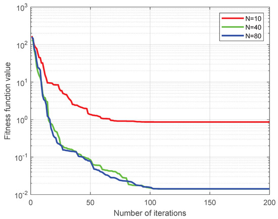
Figure 3.
Comparison of convergence performance of optimization functions with different population number N. The population number N is set to 10, 40, and 80, respectively.
Step 2: Calculate the fitness of each search point through the interferometric calibration model, find the position of the current optimal search solution and save it.
Step 3: Calculate parameters a, p and coefficient vectors A, C. Judge whether the probability p is less than 0.5. If it is, go directly to step 4. Otherwise, use Equation (20) to update the position.
Step 4: Determine whether the absolute value of the coefficient vector A is less than 1. If so, update the optimal solution position according to Equation (16); otherwise, search for the optimal solution globally at random, and update the position according to Equation (18).
Step 5: At the end of the position update, the fitness of each interferometric parameter solution is calculated and compared with the previously retained optimal interferometric parameters. If it is better than the previous optimal solution, the new optimal solution is used for replacement. Determine whether the current optimal solution is within the feasible region and use Equation (23) to dynamically update .
Step 6: Determine whether the current search number reaches the maximum number of iterations. If it reaches the optimal solution, the calculation is completed. Otherwise, enter the next iteration, and return to step 3.
Figure 4 is the flowchart of the InIRA interferometric calibration algorithm. The orange section represents the improvements we made to the original WOA evolutionary algorithm:
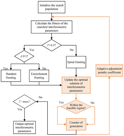
Figure 4.
The flowchart of the InIRA interferometric calibration algorithm. The orange part is our improvement of the original WOA evolutionary algorithm.
4. Experiments and Analysis
4.1. Interferometric Data Processing in the Experimental Area
The experiment uses the InIRA data borne on the Tiangong-2 space laboratory. As a near-nadir interferometric SAR, the Ku-band dual-antenna radar is used. The main system design parameters are shown in the following Table 1, where is the nearest slant distance, which is the shortest distance from the InIRA antenna to the imaging area. The data were acquired from the northern region of Qinghai Lake in Qinghai Province, China, in October 2017, and the specific geographical location is shown in the following Figure 5. We first perform basic interferometric processing on the two-channel SAR complex image [30,31]. Figure 6a is a single-channel SAR imaging amplitude image, in which the horizontal axis is the azimuth direction and the vertical axis is the range direction. It can be observed that the near-range direction is the inland area, and the far-range direction is the water body, which is the Qinghai Lake; Figure 6b is the interferometric phase image obtained after the interferometric processing of the registered SAR image, in which the interferometric phase is wrapped between 0 and . It can be observed that the interferometric fringes of the InIRA data on the water surface are similar to the interferometric fringes of the traditional InSAR on the flat ground, showing periodic characteristics. After interferometric phase filtering, Figure 6b is unwrapped by the minimum cost flow to obtain Figure 6c. Due to the short baseline design of InIRA, the interferometric phase winding is not particularly serious, and it can be unwrapped directly without removing the flat-earth phase. Figure 6d is the coherence image of the master and slave SAR images. According to the coherence, the quality of the interference in the imaging area can be judged, and the coherence is used to weight the control points in the interferometric calibration.

Table 1.
InIRA system parameters, including wavelength, baseline length, baseline inclination, nearest slant range, and incidence angle range.
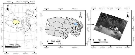
Figure 5.
The study area considered in this paper.
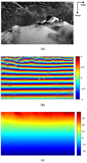
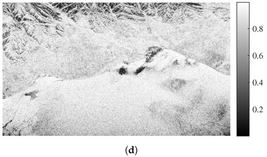
Figure 6.
Interference processing processes of the InIRA data. (a) Amplitude image; (b) interferogram image; (c) phase diagram image obtained based on the minimum cost flow unwrapping; (d) coherence image of the master and slave SAR images.
4.2. Experimental Design and Procedures
The initial physical baseline length of the InIRA is 2.3 m, and the baseline inclination is 5. This will be used as the initial parameter of the calibration, and the initial elevation is obtained based on the unwrapped interferometric phase and the phase-elevation conversion relationship. In the absence of ground control points, the reference DEM is used to assist the calibration [32,33]. The reference DEM we use is the shuttle radar topography mission (SRTM) DEM with a resolution of 30 m. In our InIRA data, the near-range direction is the land part, which can be calibrated via SRTM DEM, and the far-range direction is the water part without elevation information. Using the high coherence and high SNR characteristics of the InIRA water part, this information is used to compensate for the missing elevation information, thereby realizing the calibration of the interferometric parameters. As shown in Figure 7, in the imaging area, we select multiple SRTM elevation points along the track in the inland part as the external control points. And we select uniformly distributed elevation points on the lake as constraints. After establishing the optimization calibration model of inland water body proposed in this paper, the improved WOA algorithm is used to solve the model.
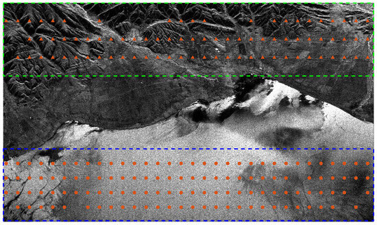
Figure 7.
The distribution of external control points on land (orange points in the green dashed box) and elevation constraint points on the lake (orange points in the blue dashed box).
At the same time, in order to increase the comparability of the experiment, we compare our proposed method with three calibration methods without ground control points: the reference DEM calibration method [18,32], the flat ground calibration method [17] and the flat-earth phase method [8]. Figure 8 shows the differences between our proposed method and the three calibration methods. The green flowchart represents the reference DEM method, which incorporates external reference DEM information to obtain corresponding external control point elevation data. It then utilizes Equation (12) for optimization to obtain the interferometric parameters. The blue flowchart represents the key steps of the flat ground calibration method, which does not involve external information but relies on the elevation characteristics of its own data. Typically, it utilizes the flatness of the terrain to construct the optimization equation and solve for the interferometric parameters. The yellow flowchart represents the flat earth phase method; it utilizes a precise correspondence between the flat earth phase and the interferometric baseline to refine the baseline accurately. Additionally, it employs polynomial fitting to mitigate errors in interferometric measurements caused by terrain deformation.
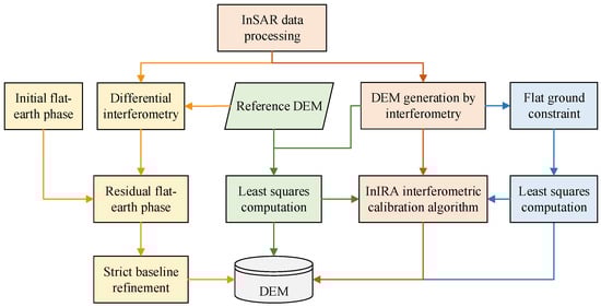
Figure 8.
Comparison flowchart of interferometric calibration methods. The green flowchart represents the reference DEM method, the blue flowchart represents the flat ground method, the yellow flowchart represents the flat earth phase method, and the pink flowchart represents the method we proposed.
To verify the proposed method, the high-precision Sentinel-3 data [34,35] in this region is used to evaluate the generated elevation. The Sentinel-3 data are independent of the external control point information we used. They have not been used in our proposed method or in the two additional methods used for comparison. Figure 9 shows the location of the elevation checkpoints on the SAR image. The Sentinel-3 data were acquired on 5 October and 1 November 2017, which closely aligns with the InIRA data acquisition time on 6 October 2017. We sampled and screened 48 elevation points as checkpoints to quantitatively analyze the generated lake elevation and land elevation. The spatial resolution of the sentinel-3 used is 300 m, and the spatial resolution of the InIRA data at the checkpoints at the far-range is about 30 m [6]. The InIRA data were spatially averaged over a window to a comparable spatial resolution to that of Sentinel-3 data.
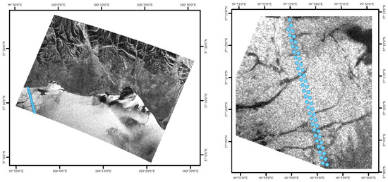
Figure 9.
The study area and the selected Sentinel-3 data for evaluation, acquired on 5 October and 1 November 2017. The image on the (right) is an enlarged view of the verification points in the (left) image.
4.3. Results and Analysis
Figure 10 depicts the distribution of generated elevation and elevation error, while Table 2 presents the quantitative comparison results between the proposed method and the other three methods. The elevation error observed when using different methods is evaluated based on three criteria: variance (VAR), average error, and root mean square error (RMSE) [36]. The reference DEM method uses inland external control points for calibration. The calibration points cannot cover the entire range direction. Therefore, it can be observed that the elevation error exhibits a slope effect, the elevation errors near the land are smaller, and the elevation error on the lake surface is particularly serious. This is because the elevation error in the area with control points is small, while the elevation error in the lake area without control points is large. The flat ground method can eliminate the range slope to some degree, but the generated elevation will have a fixed constant deviation from the actual elevation. It can be seen from the average value that the fixed elevation error is about 18.31 m, and the error variance is small. In the flat-earth phase method, the average error is −0.97 m, and there are some points with larger errors. The flat-earth phase residual is obtained by using global polynomial fitting for the interferogram, so that the flat-earth phase may absorb some other signals, which is the cause of the error. In our proposed method, the computed baseline length is 2.3359 m, the baseline inclination is 5.0382 and the absolute interferometric phase is precomputed by external DEM, and the calibration value is 0.041 rad. The range slope caused by interferometric parameter errors has been effectively eliminated, and the constant elevation error has returned to near zero value. The average elevation error is 0.31 m, with an RMSE of 1.01 m and a VAR of 0.95 m. According to these three evaluation indicators, our proposed method outperforms the other three methods, demonstrating the effectiveness of our calibration method.
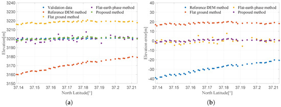
Figure 10.
Distribution of elevation values and the elevation errors at the validation points. (a) Elevation values generated by the four methods and the validation elevation values; (b) elevation errors of the four methods at the validation points.
Table 2.
Quantitative evaluation of the calibration methods.
5. Discussion
Unlike traditional InSAR measurements that focus on land surfaces with large incidence angles, InIRA can be used for both land and water body measurements. Our research area comprises both land regions and lake regions. The interferometric calibration calculation based on the adaptive constrained evolutionary algorithm we proposed is suitable for inland areas containing lakes such as InIRA images. In this case, the relative elevation flatness of the lake is used as a constraint and an adaptive penalty coefficient is used. The method we proposed is also applicable to traditional InSAR land mapping areas. At this time, when flat terrain such as plains exists, it can be used as a constraint. If it does not exist, there will be no constraint terms and the evolutionary algorithm will be used to solve it.
From Figure 6, it can be observed that we arranged calibration points on both land and the lake according to Equation (13). The number of calibration points on land is denoted as M, while the number of calibration points on the lake is denoted as N. Following the calibration point arrangement principles in interferometric calibration, calibration points on land are placed to cover the entire range direction as much as possible. If feasible, they are distributed across multiple azimuth directions to enhance stability. In our experiments, the arrangement of M calibration points on land follows the aforementioned principles.
Inspired by the calibration point layout on land, we divided the distribution of N calibration points on the lake into four categories: near-range single-range direction, far-range single-range direction, near-range multi-range direction, and far-range multi-range direction. The specific placement locations are illustrated in Figure 11. Employing these four distinct placement configurations, the proposed method in this paper is applied for processing, and the corresponding results are depicted in Figure 12. Quantitative analyses are also presented in Table 3.
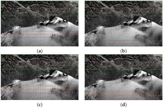
Figure 11.
Four different calibration point placement on the lake. The color of the calibration points is orange, and the calibration points on the land and the calibration points on the lake are located in the green and blue dashed boxes, respectively. (a) Near-range single-range direction placement; (b) far-range single-range direction placement; (c) near-range multi-range direction placement; (d) far-range multi-range direction placement.
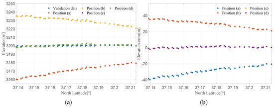
Figure 12.
Elevation values generated by the four different placement and the elevation errors at the validation points. (a) Elevation values generated by the four different placements and the validation elevation values; (b) Elevation errors of the four different placements at the validation points.
Table 3.
Quantitative evaluation of the four different calibration point placements.
We devised these four distinct calibration point placements, encompassing a comparison between near-range and far-range placement, as well as the influence of the number of control points—comparing multi-range placement to single-range placement. From Figure 12, it can be observed that placing calibration points along a single slant range on the lake still leads to the presence of the slope effect in elevation errors, with a significant variance. Placing calibration points at different slant ranges on the lake noticeably resolves the slope effect, leading to a reduction in variance and the mean value becoming very close to the validation elevation values. Across the same 48 validation points, the average error drops to 0.31 m, and the RMSE reduces to 1.01 m. These results align with the previous findings from the uniform distribution of points on the lake surface. Conclusions drawn from the results in Figure 12 and Table 3 reveal that single-range calibration points on the lake surface do not positively impact outcomes, regardless of whether they are placed near the near-range or far-range end. Multi-range placement, whether near-range or far-range, proves beneficial and exhibits similar effectiveness to placing control points across the entire lake. For stability, it is advisable to cover the entire lake with as many calibration points as possible.
6. Conclusions
This study addresses the calibration problem of short-baseline interferometric SAR with near-nadir interference. Firstly, we analyze the impact of interferometric parameters on elevation errors and find through system simulation that these parameters have a linear impact on elevation within the error range, and that there is severe coupling among them. Next, we propose a calibration model based on inland water bodies without ground control points due to the high coherence of backscattering signals on water surfaces in InIRA data. The relative flatness of the lake surface is used as an inequality constraint to compensate for the missing information of the lake part without ground control points. To solve this calibration model, we introduce an intelligent evolutionary algorithm. The model’s constraint ability is adaptively adjusted during the iteration process, and the WOA algorithm’s global search ability and wide search range are utilized to avoid local optimal points, thus determining optimal interferometric parameters and achieving high-precision inland water level generation. Through comparisons with several other calibration methods, the effectiveness and advantages of our proposed approach have been demonstrated.
Our study does not consider changes in baseline with azimuth time. Therefore, the next step is to investigate the characteristics of InIRA baseline with azimuth time and develop an accurate model to enable more precise generation of inland and lake elevations.
Author Contributions
Conceptualization, B.W., H.T., M.X. and L.L.; methodology, B.W. and L.L.; software, L.L., K.W. and Y.W.; writing—original draft preparation, L.L.; writing—review and editing, L.L., B.W., Y.W., K.W. and H.T. All authors have read and agreed to the published version of the manuscript.
Funding
This work was supported by the National Natural Science Foundation of China under Grant 41971329.
Data Availability Statement
The data presented in this study are available on request from the corresponding author. The data are not publicly available due to confidentiality of the data.
Acknowledgments
Thanks to China Manned Space Engineering for providing space science and application data products from Tiangong-2.
Conflicts of Interest
The authors declare no conflict of interest.
References
- Fu, L.L.; Cazenave, A. Satellite Altimetry and Earth Sciences: A Handbook of Techniques and Applications; Elsevier: Amsterdam, The Netherlands, 2000. [Google Scholar]
- Tapley, B.D.; Born, G.H.; Parke, M.E. The Seasat altimeter data and its accuracy assessment. J. Geophys. Res. Ocean. 1982, 87, 3179–3188. [Google Scholar] [CrossRef]
- Cheney, R.E.; Douglas, B.C.; Miller, L. Evaluation of Geosat altimeter data with application to tropical Pacific sea level variability. J. Geophys. Res. Ocean. 1989, 94, 4737–4747. [Google Scholar] [CrossRef]
- Biancamaria, S.; Schaedele, T.; Blumstein, D.; Frappart, F.; Boy, F.; Desjonquères, J.D.; Pottier, C.; Blarel, F.; Niño, F. Validation of Jason-3 tracking modes over French rivers. Remote Sens. Environ. 2018, 209, 77–89. [Google Scholar] [CrossRef]
- Bonnefond, P.; Laurain, O.; Exertier, P.; Boy, F.; Guinle, T.; Picot, N.; Labroue, S.; Raynal, M.; Donlon, C.; Féménias, P.; et al. Calibrating the SAR SSH of Sentinel-3A and CryoSat-2 over the Corsica Facilities. Remote Sens. 2018, 10, 92. [Google Scholar] [CrossRef]
- Kong, W.; Chong, J.; Tan, H. Performance analysis of ocean surface topography altimetry by Ku-band near-nadir interferometric SAR. Remote Sens. 2017, 9, 933. [Google Scholar] [CrossRef]
- Chaudhary, A.; Agarwal, N.; Sharma, R.; Ojha, S.P.; Kumar, R. Nadir altimetry Vis-à-Vis swath altimetry: A study in the context of SWOT mission for the Bay of Bengal. Remote Sens. Environ. 2021, 252, 112120. [Google Scholar] [CrossRef]
- Xu, B.; Li, Z.; Zhu, Y.; Shi, J.; Feng, G. SAR interferometric baseline refinement based on flat-earth phase without a ground control point. Remote Sens. 2020, 12, 233. [Google Scholar] [CrossRef]
- Otten, M.; Dow, J. Envisat Precise Orbit Determination. In Proceedings of the Envisat & ERS Symposium, Salzburg, Austria, 6–10 September 2005; Volume 572. [Google Scholar]
- Scharroo, R.; Visser, P. Precise orbit determination and gravity field improvement for the ERS satellites. J. Geophys. Res. Ocean. 1998, 103, 8113–8127. [Google Scholar] [CrossRef]
- Small, D.; Werner, C.; Nuesch, D. Baseline modelling for ERS-1 SAR interferometry. In Proceedings of the IGARSS’93-IEEE International Geoscience and Remote Sensing Symposium, Tokyo, Japan, 18–21 August 1993; pp. 1204–1206. [Google Scholar]
- Joughin, I.; Winebrenner, D.; Fahnestock, M.; Kwok, R.; Krabill, W. Measurement of ice-sheet topography using satellite-radar interferometry. J. Glaciol. 1996, 42, 10–22. [Google Scholar] [CrossRef]
- Kimura, H.; Todo, M. Baseline estimation using ground points for interferometric SAR. In Proceedings of the IGARSS’97. 1997 IEEE International Geoscience and Remote Sensing Symposium Proceedings. Remote Sensing-A Scientific Vision for Sustainable Development, Singapore, 3–8 August 1997; Volume 1, pp. 442–444. [Google Scholar]
- Liu, G. Monitoring of Ground Deformations with Radar Interferometry; Surveying and Mapping Press: Austin, TX, USA, 2006. [Google Scholar]
- Li, X.; Guo, H.; Liao, J.; Wang, C.; Fan, D. Baseline estimation of interferometric SAR based on fast fourier transform. Acta Geod. Cartogr. Sin. 2003, 32, 70–72. [Google Scholar]
- Dall, J.; Christensen, E.L. Interferometric calibration with natural distributed targets. In Proceedings of the IEEE International Geoscience and Remote Sensing Symposium, Toronto, ON, Canada, 24–28 June 2002; Volume 1, pp. 170–172. [Google Scholar]
- Zhang, W.; Xiang, M.; Wu, Y. Interferometric SAR calibration with area calibration site of same height. In Proceedings of the 2009 IEEE International Geoscience and Remote Sensing Symposium, Cape Town, South Africa, 12–17 July 2009; Volume 4, pp. IV-554–IV-557. [Google Scholar]
- Mao, Y.; Xiang, M.; Han, Y.; Gao, W. Weighted joint calibration for interferometric SAR. J. Syst. Eng. Electron. 2013, 24, 761–771. [Google Scholar] [CrossRef]
- Jun, F.; Tao, L.; Xiaoqing, Z.; Qianfu, C.; Xiang, Z.; Jing, L. Interferometric calibration method for spaceborne SAR based on independent parameter decomposition. Acta Geod. Cartogr. Sin. 2019, 48, 737. [Google Scholar]
- González, J.H.; Bachmann, M.; Krieger, G.; Fiedler, H. Development of the TanDEM-X calibration concept: Analysis of systematic errors. IEEE Trans. Geosci. Remote Sens. 2009, 48, 716–726. [Google Scholar] [CrossRef]
- Adeli, H.; Cheng, N.T. Integrated genetic algorithm for optimization of space structures. J. Aerosp. Eng. 1993, 6, 315–328. [Google Scholar] [CrossRef]
- Guo, P.; Wang, X.; Han, Y. The enhanced genetic algorithms for the optimization design. In Proceedings of the 2010 3rd International Conference on Biomedical Engineering and Informatics, Yantai, China, 16–18 October 2010; Volume 7, pp. 2990–2994. [Google Scholar]
- Wang, Q. Using genetic algorithms to optimise model parameters. Environ. Model. Softw. 1997, 12, 27–34. [Google Scholar] [CrossRef]
- Beck, A.; Ben-Tal, A.; Teboulle, M. Finding a global optimal solution for a quadratically constrained fractional quadratic problem with applications to the regularized total least squares. SIAM J. Matrix Anal. Appl. 2006, 28, 425–445. [Google Scholar] [CrossRef]
- Gravelle, H.; Rees, R. Microeconomics; Pearson Education: London, UK, 2004. [Google Scholar]
- Tang, W.; Huang, L.; Liu, A. An Optimized Design of the Interferometric Calibration Method Based on Genetic Algorithm. In Proceedings of the 2019 6th Asia-Pacific Conference on Synthetic Aperture Radar (APSAR), Xiamen, China, 26–29 November 2019; pp. 1–5. [Google Scholar] [CrossRef]
- Vikhar, P.A. Evolutionary algorithms: A critical review and its future prospects. In Proceedings of the 2016 International Conference on Global Trends in Signal Processing, Information Computing and Communication (ICGTSPICC), Jalgaon, India, 22–24 December 2016; pp. 261–265. [Google Scholar]
- Mirjalili, S.; Lewis, A. The whale optimization algorithm. Adv. Eng. Softw. 2016, 95, 51–67. [Google Scholar] [CrossRef]
- Gharehchopogh, F.S.; Gholizadeh, H. A comprehensive survey: Whale Optimization Algorithm and its applications. Swarm Evol. Comput. 2019, 48, 1–24. [Google Scholar] [CrossRef]
- Chen, Y.; Zhang, G.; Ding, X.; Li, Z. Monitoring earth surface deformations with InSAR technology: Principles and some critical issues. J. Geospat. Eng. 2000, 2, 3–22. [Google Scholar]
- Ma, F.; Sun, X.; Zhang, F.; Zhou, Y.; Li, H.C. What Catch Your Attention in SAR Images: Saliency Detection Based on Soft-Superpixel Lacunarity Cue. IEEE Trans. Geosci. Remote Sens. 2023, 61, 1–17. [Google Scholar] [CrossRef]
- Yun, Y.; Zeng, Q.; Jiao, J.; Liang, C.; Wang, Q.; Zhou, X.; Yan, D. Calibration of airborne interferometric SAR data by external dem without artificial calibrators. In Proceedings of the 2012 IEEE International Geoscience and Remote Sensing Symposium, Munich, Germany, 22–27 July 2012; pp. 4501–4504. [Google Scholar]
- Yu, Y.; Jin, G.; Xiong, X.; Tong, C.; Zhang, G. SAR elevation control point extraction combining multistrategy ATLAS data preference and image matching. J. Radars 2023, 12, 64. [Google Scholar]
- Zhang, X.; Jiang, L.; Kittel, C.M.; Yao, Z.; Nielsen, K.; Liu, Z.; Wang, R.; Liu, J.; Andersen, O.B.; Bauer-Gottwein, P. On the performance of Sentinel-3 altimetry over new reservoirs: Approaches to determine onboard a priori elevation. Geophys. Res. Lett. 2020, 47, e2020GL088770. [Google Scholar] [CrossRef]
- Jiang, L.; Nielsen, K.; Dinardo, S.; Andersen, O.B.; Bauer-Gottwein, P. Evaluation of Sentinel-3 SRAL SAR altimetry over Chinese rivers. Remote Sens. Environ. 2020, 237, 111546. [Google Scholar] [CrossRef]
- Aguilar, F.J.; Agüera, F.; Aguilar, M.A.; Carvajal, F. Effects of terrain morphology, sampling density, and interpolation methods on grid DEM accuracy. Photogramm. Eng. Remote Sens. 2005, 71, 805–816. [Google Scholar] [CrossRef]
Disclaimer/Publisher’s Note: The statements, opinions and data contained in all publications are solely those of the individual author(s) and contributor(s) and not of MDPI and/or the editor(s). MDPI and/or the editor(s) disclaim responsibility for any injury to people or property resulting from any ideas, methods, instructions or products referred to in the content. |
© 2023 by the authors. Licensee MDPI, Basel, Switzerland. This article is an open access article distributed under the terms and conditions of the Creative Commons Attribution (CC BY) license (https://creativecommons.org/licenses/by/4.0/).