Article

Multi-Stage Semantic Segmentation Quantifies Fragmentation of Small Habitats at a Landscape Scale

by
Thijs L. van der Plas
1,2,
Simon T. Geikie
2,
David G. Alexander
2,† and
Daniel M. Simms
3,*,†
1
Doctoral Training Centre, University of Oxford, Oxford OX1 3NP, UK
2
Peak District National Park Authority, Bakewell DE45 1AE, UK
3
Applied Remote Sensing Group, Cranfield University, Cranfield MK43 0AL, UK
*
Author to whom correspondence should be addressed.
Co-senior author.
Remote Sens. 2023, 15(22), 5277; https://doi.org/10.3390/rs15225277
Submission received: 9 October 2023 / Revised: 3 November 2023 / Accepted: 4 November 2023 / Published: 7 November 2023

Abstract

:
Land cover (LC) maps are used extensively for nature conservation and landscape planning, but low spatial resolution and coarse LC schemas typically limit their applicability to large, broadly defined habitats. In order to target smaller and more-specific habitats, LC maps must be developed at high resolution and fine class detail using automated methods that can efficiently scale to large areas of interest. In this work, we present a Machine Learning approach that addresses this challenge. First, we developed a multi-stage semantic segmentation approach that uses Convolutional Neural Networks (CNNs) to classify LC across the Peak District National Park (PDNP, 1439 km2) in the UK using a detailed, hierarchical LC schema. High-level classes were predicted with 95% accuracy and were subsequently used as masks to predict low-level classes with 72% to 92% accuracy. Next, we used these predictions to analyse the degree and distribution of fragmentation of one specific habitat—wet grassland and rush pasture—at the landscape scale in the PDNP. We found that fragmentation varied across areas designated as primary habitat, highlighting the importance of high-resolution LC maps provided by CNN-powered analysis for nature conservation.

1. Introduction

Land cover (LC) maps are essential tools for measuring and monitoring the state of natural landscapes [1]. Their applicability to landscape ecology [2,3], climate change vulnerability [4,5], natural capital and ecosystem service assessments [6,7] or conservation work [8] is largely determined by their resolution and accuracy.
High-resolution LC maps were historically produced by detailed ground surveys or drawn by hand from photo-interpretation of aerial imagery [9,10]. Machine Learning (ML) image classification methods, such as Random Forests and Support Vector Machines, have since been used for automating these labour-intensive manual approaches at a range of scales and across different habitats [11,12,13]. These relatively simple ML approaches typically require extensive image pre-processing and feature engineering to create input data with sufficiently low intra-class variability, incorporating spatial features through texture analysis or grouping pixels into objects using image segmentation. To overcome these limitations, deep learning models using Convolutional Neural Networks (CNNs) learn spatial patterns directly from raw imagery, which enables models to be applied efficiently at scale [14].
The spatial resolution of LC maps is determined by the ground resolution of the image data, which is typically upward of 10 m for public satellite data [15]. Although sufficient for some purposes, commonly available coarse-resolution LC maps preclude the accurate surveying and monitoring of small-scale, patchily distributed habitats and of fragmented or mosaic habitats at a landscape scale [16]. To address this, unmanned aerial vehicles (UAVs) are increasingly used to collect very-high-resolution images for mapping LC at a high level of detail [17]. Whilst advances in deep learning show great promise for combining UAVs and Machine Learning analysis [18,19], issues with weather conditions, operational factors and consumer-grade sensors or cameras remain, which makes operating UAVs at a landscape scale impractical [20].
Alternatively, aerial surveys from piloted aircraft provide a compromise between high-resolution imagery and large spatial coverage, resulting in greater consistency of imagery at a landscape scale [20]. In addition to spatial resolution, another key feature of LC maps is their LC class resolution—i.e., the specificity of the LC class schema. For example, European LC maps categorise habitats into relatively broad classes (forest, water, fields, etc.), which are useful for generalised LC monitoring [21], but this reduced thematic detail results in landscape characteristics being defined less precisely [22]. Within the United Kingdom (UK), current nationally available LC data sets such as the Centre of Ecology and Hydrology [23] or the Living England [24] LC maps provide context for LC classes and spatial resolution needed at a national level but do not provide regional information tailored to a specific area of interest [25].
In this study, we consider the Peak District National Park (PDNP) in the UK, where the need for a high spatial and class resolution LC map is particularly relevant. The PDNP is an International Union for Conservation of Nature (IUCN) Category V Protected Area, characterised by the interaction of people (such as farming, housing, tourism and industry) and nature over time [26]. As such, this has created a mixed landscape of farmland and other developed land along with sites designated primarily for nature conservation and other land uses [27]. Landscape management planning therefore operates over large spatial scales, addressing a range of ecosystem processes, conservation objectives and land uses [28]. Nevertheless, in the UK, there remains limited coverage of high-resolution LC data sets to support the delivery of landscape-scale conservation objectives, evidenced by the fact that the last time LC was extensively surveyed and classified in National Parks (NPs) was in 1991 by visual interpretation of aerial photography [9].
Here, we have adapted (and slightly updated) the 1991 schema to create a new LC map of the PDNP using CNN-based semantic segmentation. However, two challenges must be overcome in order to use CNNs to predict the small-scale variations in LC typically found in UK NPs. Firstly, both raw and annotated data must be available at very high resolution. Second, CNNs must be able to handle the strongly non-uniform distribution of LC classes as well as the inherent variability of large-scale aerial photography related to image capture, such as the time of day and seasonality [11].
We have addressed these two challenges by (1) creating a very-high-resolution data set and (2) developing a multi-stage CNN semantic segmentation approach. To overcome the first challenge, we have created an extensive data set of over 1000 image patches of 64 m × 64 m at 12.5 cm ground resolution and manually annotated using an updated version of the LC schema from [9,29]. LC classes range from woodland subclasses to moorland mosaics, and patches are distributed across the entire PDNP (spanning 1439 km2). We have made this data set publicly available, including the raw RGB data [30], which we envision could become a new standard data set for benchmarking UK LC prediction models. Secondly, we developed a multi-stage approach to overcome the challenge of non-uniform LC classes. We trained CNNs to classify RGB aerial photography obtained at 12.5 cm ground resolution [30], and leveraging the multi-level structure of the hierarchical LC schema, we first predicted high-level classes, which we then used as a mask to predict their low-level subclasses. We then overlaid model predictions with a topography layer of urban classes [31] to generate highly detailed LC maps. Further, secondary data were used to aid classification between some subclasses (using soil data).
Finally, we demonstrate the applicability of this model by quantifying metrics of habitat fragmentation of wet grassland and rush pasture across designated primary habitat areas. In summary, by developing a multi-stage approach to train CNNs and creating a detailed LC data set, we were able to detect small-scale LC features across landscapes at scales that are fine enough to inform local management decisions.

2. Methods

2.1. Study Area

This study concerns the Peak District National Park (PDNP), England, United Kingdom, which totals 1439 km2 (see Figure 1). The PDNP is an upland area at the southern end of the Pennines, most of which is above 300 m in altitude and with the highest point at 636 m. The PDNP contains a variety of landscapes that range from largely uninhabited broad, open moorlands in the Dark Peak [32] to more-enclosed farmlands and wooded valleys in the White Peak and South West Peak [32]. The landscapes have been shaped by variations in geology and landform and the long settlement and use of these landscapes by people.

2.2. Image Data

Orthorectified aerial digital photography of the entire PDNP (1439 km 2 ) was obtained at 12.5 cm ground resolution through the Aerial Photography Great Britain (APGB) agreement for UK public sector bodies [30]. Standard aerial photography images were used, containing red, green, and blue (RGB) wide spectral channels and collected at seven different dates between April 2019 to June 2022 (Figure 1b).

2.3. Convolutional Neural Network

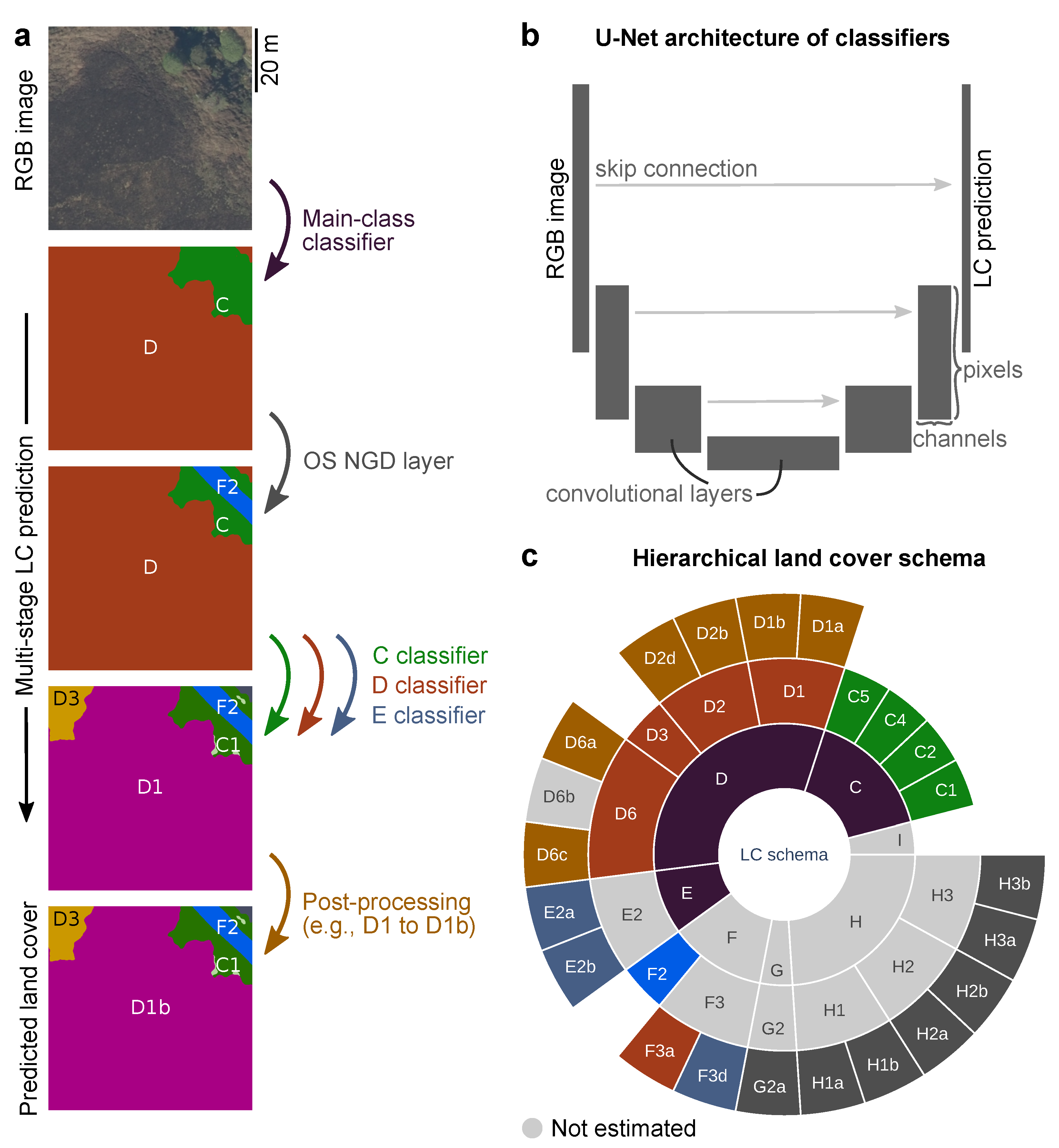
Convolutional Neural Networks (CNNs) are deep neural networks that use convolutional layers that can efficiently process image data; they have a strong track record in remote sensing and ecology applications [14,33]. In this study, we consider the task of performing semantic segmentation, i.e., predicting the (LC) class for each pixel of the input RGB image. To this end, we used a CNN model specialised for this task: the U-Net [14,34,35,36]. U-Nets are characterised by their (U-shaped) layout of hidden layers (Figure 2b). First, a stack of encoding convolutional layers abstracts task-relevant information from the input image, which is then used by decoding layers to predict the LC class of each pixel. We used U-Nets adapted from Iakubovskii [37], which were pretrained on Imagenet prior to optimisation on this task to reduce training time and the required number of data points. All classifiers used the same model architecture and training parameters (see Section 2.7).

2.4. Land Cover Schema

The landscape classification system used to classify the area features originated from the Monitoring Landscape Change in England and Wales survey undertaken by Hunting Technical Services Ltd. (1986) [29]. This was a national classification suitable for mapping UK habitats from a combination of ground surveys and aerial photographs. Modifications were made to the classification categories by Taylor et al. [9,29] to take into account more-specialised LC classes found in UK national parks and that those features were solely mapped from aerial photography. This schema is representative of the landscape within the UK and is well-suited for monitoring LC classes in the PDNP and other UK national parks and surveying in detail single species, mixed species classes or intensively managed areas [38].
We further adapted the land cover schema from Taylor et al. [9,29], with the addition of a new wetland vegetation class (F3d, wet grassland and rush pasture) and an extra subclass of upland heath (D1b, peaty soil upland heath): see Table 1. Wet grassland and rush pasture (F3d) occurs on poorly drained, usually acidic soils and contributes to the richness of invertebrate fauna supporting key species. The habitat consists of various species-rich types of fen meadow and rush pasture such as purple moor grass (Molinia caerulea) and rushes, especially sharp-flowered rush (Juncus acutiflorus). In the landscape, it can often be found fragmented as part of the mosaic of farmland habitats and also moorland areas. Because of this, the habitat does not represent a fixed phytosociological community [39], but as a land cover class, it is of interest as it is a cosmopolitan, patchily distributed habitat across the whole study area that occurs both within areas of moorland (D) and grassland (E). Therefore, it was decided to include it in both the D and E classifiers (see Section 2.8).
Table 1. Land cover schema adapted from [9,10,29]. LC80 is the original schema; LC20 is the updated schema that we have created. LC80-main denotes the main class. Only classes that are present in PDNP are included.
LC80-MainLC80LC20NameNew?
C (Wood and forest land)C1C1Broadleaved high forest-
CC2C2Coniferous high forest-
CC4C4Scrub-
CC5C5Clear felled/newly planted trees-
D (Moor and heath land)D1D1aUpland heath-
DD1D1bUpland heath, peaty soilYes
DD2bD2bUpland grass moor-
DD2dD2dBlanket peat grass moor-
DD3D3Bracken..
DD6aD6aUpland heath/grass mosaic-
DD6cD6cUpland heath/blanket peat mosaic-
E (Agro-pastoral land)E2aE2aImproved pasture-
EE2bE2bRough pasture-
F (Water and wetland)F2F2Open water, inland-
FF3aF3aPeat bog-
FD2/E2F3dWet grassland and rush pastureYes
G (Rock and coastal land)G2G2Inland bare rock-
H (Developed land)H1aH1aUrban area-
HH1bH1bMajor transport route-
HH2aH2aQuarries and mineral working-
HH2bH2bDerelict land-
HH3aH3aIsolated farmsteads-
HH3bH3bOther developed land-
I (Unclassified land)IIUnclassified land-
Some LC classes from the schema by [9,29] were excluded in this study; the reasons for the exclusions are as follows:
  • C3 (mixed high forest)—the aim of the new modelling was to resolve C1 (broadleaved) and C2 (coniferous) at the resolution of single trees, so it was decided to exclude C3 (which would normally consider large parcels of woodlands to be a mix of broadleaved and coniferous trees).
  • D4 (unenclosed lowland areas)—the distinction between D4 and E classes is based on whether the land is “enclosed for stock control purposes” [29]. This cannot be done based on 64 m × 64 m image patches as used for input data by the CNNs. D4 was therefore excluded.
  • D6b (upland mosaic heath/bracken)—although we have labelled these areas in the train/test data sets, we decided to merge these areas after classification into D3 (bracken). This was done because both D3 and D6b were relatively rare and therefore difficult to learn, while together they provided more data points (though combined, this was still one of the rarest classes).
  • D7 (eroded areas)—the large areas of eroded peat (D7a) that were present in the Peak District in the 1991 census [9] have now been revegetated by the establishment of grasses and moorland plants in the past decades [20,40]. The few remaining patches of eroded peat are typically small patches or narrow strips in the bases of gullies.
  • D8 (coastal heath)—not present in the Peak District.
  • E1 (cultivated land)—this is barely present in the Peak District and was therefore excluded. (And where still present, it is relabelled to E2a).
  • F1 (coastal open water), F3b (freshwater marsh), F3c (saltmarsh), G2b (coastal rock) and G3 (other coastal features)—all not present in the Peak District.
The final schema is illustrated in Figure 2b and detailed in Table 1. To facilitate further use of these data and this schema, we have created an interpretation key with example images of each class, available at https://reports.peakdistrict.gov.uk/interpretation-key/docs/introduction.html (accessed on 27 September 2023) [38].

2.5. Selecting Image Patches for Training and Testing

The image data were available as 1 km × 1 km tiles, which were split into 64 m × 64 m (i.e., 512 pixels × 512 pixels) patches for input to the CNN models. Our goal was to create a data set that sufficiently covered the spatial extent of the PDNP, the variety in LC classes, the variability within LC classes and the variability in image acquisition across different regions (caused by different flight dates). We therefore selected image patches across the PDNP with the following procedure:
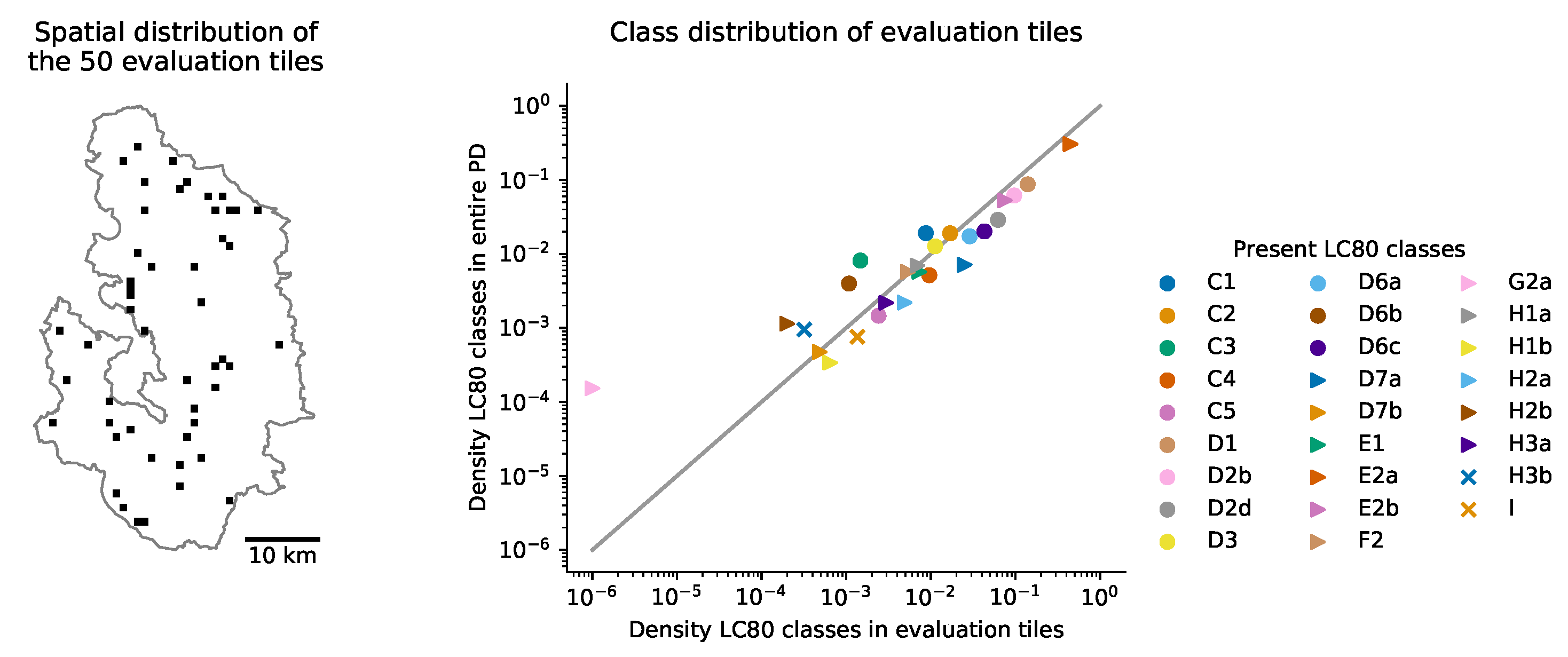
First, we used the 1991 census data [9] to select 50 tiles (of 1 km2 each) that were representative of the overall LC distribution (of 1991). To do so, we generated 50,000 random samples of 50 tiles, computed the L1 loss of the LC area distribution of the sample compared to the LC area distribution of the entire PDNP, and selected the sample with the lowest L1 loss. This resulted in a sample of 50 tiles that was spatially distributed across the PDNP, illustrated in Figure 3. From each of these tiles, we randomly selected nine image patches (of 64 m × 64 m)—one from each block of a 3 × 3 grid across the tile—resulting in 450 image patches. This approach was used to prevent bias in sample selection and to ensure the accuracy metrics used for validation were representative of the final mapped outputs [41]. However, some classes are much more prevalent than others (Figure 3). This meant that rare classes were very unlikely to be sampled sufficiently for model training. Therefore, an additional 577 patches were selected manually across the same 50 tiles, plus 30 extra tiles were selected to boost rare classes (Figure 1c).
For the purpose of training a model that predicts land cover, we distinguish the following three types of data:
  • Training: (geospatial) data that are used to train the CNN classification models. These consist of both input data (aerial imagery) and land cover annotations.
  • Testing: data that are used to evaluate the performance of trained CNNs. Importantly, these data are not used to further improve CNN performance nor to assess convergence but only to quantify its final performance. These consist of both input imagery and land cover annotations.
  • Prediction: this is the entire area that is classified with the converged model (for further analysis). Only input imagery data are available a priori, from which the model predicts the land cover annotations.

2.6. Land Cover Annotation

The 1027 patches (64 m × 64 m) selected for training and testing the models were annotated manually by image-interpretation according to the LC schema of Table 1. We labelled land cover using visual interpretation of aerial images because this allowed us to draw accurate LC class boundaries consistently at scale. Annotations were first done by one human expert interpreter, and afterwards, they were checked (and corrected where necessary) by a second expert interpreter. Uncertain annotations were verified in the field, leading to a highly detailed and accurate data set representative of upland UK landscapes. This data set was split randomly into 70% for training and 30% for testing the CNN models. The same split was used for all models and is maintained in the public data set [42].
We used publicly available woodlands data to aid and speed up the manual annotation of large woodlands in image patches [43]. Further, OS NGD data were used for mapping the F2, G2a and H classes (Figure 2, [31]). Lastly, primary habitat data for wet grassland and rush pasture were used for the habitat fragmentation analysis [44]. These are all summarised in Table 2.

2.7. Model Training

We explored two popular CNN backbones [14], Resnet50 and Efficientnet-b1 [37], and observed after visual inspection of large areas of predictions (continuous areas larger than single 64 m × 64 m patches) that Efficientnet had the tendency to classify patches as a whole, despite adding overlap (padding) between image patches, leading to block-like predictions at a large scale (see Figure 4 for an example). It was therefore decided to use Resnet50 networks going forward. All CNNs were trained for 60 epochs using a batch size of 10, after which, the best-performing iteration based on the training loss was selected. Next, we considered two loss functions (cross entropy and focal loss with γ = 0.75 ), and optimised five CNNs for each loss function using an Adam optimizer for all four classifiers (main, C, D and E). Table 3 reports the mean, standard deviation and maximum of the accuracy across the five runs for each setting. The best (i.e., maximum accuracy) model was then selected for the final predictions.
CNNs received RGB image patches of 512 × 512 pixels as input. To avoid edge effects, we used a padding of 22 pixels (meaning neighbouring image patches slightly overlapped). Image patches were grouped per tile of 1000 m × 1000 m, so the edges of these tiles were predicted without overlap. Input images were z-scored, and during training, data were augmented by random horizontal and/or vertical flipping. For training the main classifiers, LC annotations were relabelled to their corresponding main class (e.g., C1 was relabelled to C). For training the detailed classifiers, LC annotations that were not relevant to the classifier (e.g., C1 is not relevant to the D classifier) were blanked out and did not contribute to the loss during training.

2.8. Multi-Stage Semantic Segmentation

We developed a multi-stage approach because of the hierarchical LC schema, the high number of classes (23), the strong non-uniformity of the class distribution (Figure 3) and the intra-class variance caused by the large area of interest (PDNP, 1439 km2). The classification process was split into four stages (Figure 2a). First, one CNN model was used to predict the main classes directly from the RGB data (Figure 2a, first step). Second, OS NGD data were used to overwrite these predictions with any F2 (open water), G (rock) or H (developed land) LC class (Figure 2a, second step). Third, three separate CNN classifiers were used for the prediction of the detailed sub-classes (Figure 2a, third step). These detailed predictions were then masked using the combined classes from the previous step. For example, the output of the C-classifier would predict, directly from the RGB data, detailed C1, C2, C4 and C5 classes (see Table 1) at locations classified as C by the main classifier. Fourth, soil data [45] were used to disambiguate between subclasses of D (moorlands) with or without peaty soil: e.g., D1a or D1b (Figure 2a, fourth step).
The new LC class wet grassland and rush pasture (F3d) posed a challenge for the classifiers, as it typically occurs in small patches both within moorlands (D) and grasslands (E). As CNNs rely on the context of the RGB image for classification, these different types of habitat surroundings were initially found to confuse the CNN models. Therefore, we decided to: (1) include F3d as a category in both the detailed D classifier and the detailed E classifier and (2) for the purpose of training the main classifier only, remap any F3d polygons to D class. In other words, to the CNN classifiers, F3d was presented as a subclass of D (moorlands) while allowing the possibility to classify E (grasslands) into F3d given its presence in grasslands too.

2.9. Single-Stage Semantic Segmentation

For comparison with the multi-stage models, detailed LC classes were also predicted directly using conventional single-stage semantic segmentation. U-Nets were trained using exactly the same protocols and parameters as previously described. Again, five networks were trained, and the best-performing network was selected for further analysis (Table 3). Networks were trained to predict the detailed LC classes directly.

2.10. Merger with OS Layer for Developed Land

Ordnance Survey (OS) data were used to map the water (F2), rock (G2) and developed land (H) classes, as these had already been accurately and recently mapped by Ordnance Survey [31]. After the main classifier predicted the main class of the land cover, these predictions were overwritten by the OS layer (i.e., areas that contained OS polygons replaced the model-predicted polygons, Figure 2a). To do so, OS polygon classes were relabelled to our LC schema (the relabelling key is available online: https://github.com/pdnpa/cnn-land-cover/blob/main/content/os_to_lc_mapping.json, accessed on 5 November 2023). Quarry (H2a) OS annotations were found to be inaccurate, and therefore, they were all manually verified and deleted if necessary.

2.11. Post-Processing of Model Predictions

Some detailed classes were distinguished based on secondary soil data (Figure 2a). Specifically, some D classes had peat-soil and non-peat-soil variants (D1a and D1b, D2b and D2d, and D6a and D6c). To identify these, the model predicted D1, D2 and D6 generally, and predictions were subsequently labelled as peat/non-peat based on the `Peaty Soils Location’ data set from Natural England [45]. For each predicted D1, D2 and D6 polygon, the intersection with the peaty soils layer polygons was computed, and it was then assigned the peat label if the intersection was greater than 50% of the area of the predicted polygon.
However, model predictions in the paper are shown without this post-processing step, as it is a deterministic separation of some classes that does not change the performance or accuracy of any class (but does create extra classes).

2.12. Statistics

All CNN models were evaluated on withheld test data only (30% of the 1027 image patches in our data set—the same train/test split was used for all models and analyses throughout this study). Predictions were evaluated by pixel-wise comparison between the human-annotated LC labels and the model-predicted LC labels. The following evaluation metrics were used, where TP = true positive, FP = false positive and FN = false negative predicted pixels, and c indexes the LC class (e.g., C1, C2, …):
sensitivity c = T P c T P c + F N c , precision c = T P c T P c + F P c
Further, the overall accuracy of a CNN classifier was computed as:
accuracy = c T P c T P c + F N c = c T P c T P c + F P c

2.13. Habitat Fragmentation Indices

Wet grassland and rush pasture provides a relevant case study for the application of our model because, whilst fragmented and patchily distributed across the broader landscape, in total it covers a large area within the PDNP. Understanding the patch density, distribution and other structural properties of such fragmented habitats at fine scales could help to inform future management objectives and form the basis of monitoring projects. The most obvious components of this class are the rushes (Juncus spp.)—all plant names follow [46]—purple moor grass (Molinea caerulea) and sedges (Carex spp.), which are clearly visible in aerial imagery at the scale used here [47].
To quantify the habitat fragmentation of wet grassland and rush pasture habitat (F3d), we focused on the cluster of F3d habitats in the South West Peak [32]. We used the GIS layer of Habitat Networks by Natural England [44] and selected the “Purple Moor Grass & Rush Pasture” habitats that occurred within the PDNP. We then evaluated our model predictions within these `Primary Habitat’ (PH) polygons from Natural England [44] and, in particular, the model-predicted F3d polygons. (Model-predicted F3d polygons that extended across the boundary of PH polygons were cut off at the boundary except for the analysis of the buffer zone (see below)).
The following metrics were used for the analysis of habitat fragmentation:
  • Area of F3d in habitat polygon (fraction): total area of model-predicted F3d polygons inside one PH polygon.
  • Total F3d edge length normalised by habitat area (1/km): sum of edge lengths of model-predicted F3d polygons inside one PH polygon divided by the area of that one PH polygon.
  • Average nearest neighbour distance (km): average nearest-neighbour distance between model-predicted F3d polygons inside one PH polygon. PH polygons with fewer than two model-predicted F3d polygons were ignored.
  • Number of predicted F3d polygons: number of model-predicted F3d polygons inside one PH polygon.
  • Area of habitat polygon (km2): total area of one PH polygon.
  • Average global isolation (km): average of global distance of all model-predicted F3d polygons inside one PH polygon, where global distance is the mean distance of the focal model-predicted F3d polygon to all other model-predicted F3d polygons (inside that PH polygon).
  • Habitat polygon edge length (km): total edge length of one PH polygon.
  • Total area F3d in 50 m buffer (km2): total area of model-predicted F3d within the 50 m buffer zone around one PH polygon.

2.14. Data and Software Availability

The Convolutional Neural Networks (CNNs) were trained in Python 3.7 using Pytorch as the automatic differentiation package [48]. All code is available at https://github.com/pdnpa/cnn-land-cover, accessed on 5 November 2023.
QGIS 3.26 and ArcGIS 3.1.2 were used as the GIS software and for map compositions. Other figures were made using matplotlib [49], plotly and Inkscape 0.92.
We have made the train and test data sets of RGB images and land cover annotations publicly available [42]. We have also written an interpretation key with example images and descriptions of each habitat [38]. The model-predicted land cover of the entire PDNP is available upon request.

3. Results

3.1. Multi-Stage Semantic Segmentation

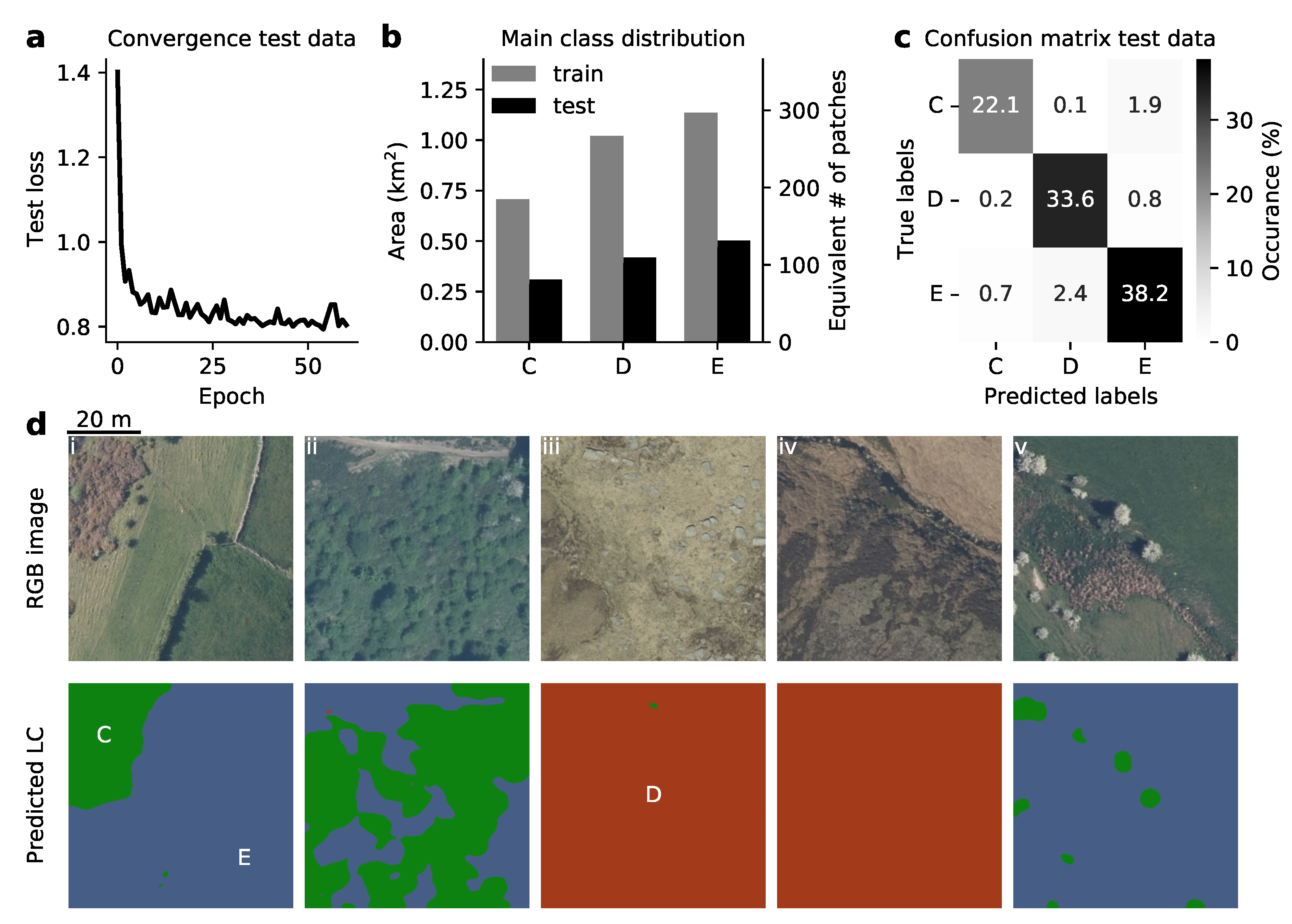
We created a new data set of LC annotated RGB images at 12.5 cm resolution, which we have made publicly available [42]. We first trained CNNs to classify the RGB images into the three main (natural) classes of our LC scheme: woodlands (C), moorlands (D) and grasslands (E), which successfully converged (Figure 5a, Table 3). CNN performance was very accurate for all classes, reaching 95% accuracy overall (Figure 5b,c and Table 4).
Example image patches demonstrate the segmentation precision of these CNN predictions (Figure 5d). Class boundaries are drawn accurately, and very small features such as single trees (Figure 5d–v) are detected well. These visual assessments are corroborated by quantifying the performance on the entire test set: sensitivity and precision are above 0.9 for all classes (Table 4). This high level of accuracy for all classes is crucial for the dual-classification approach that we use: segmentation of subclasses is only valid once a very high level of accuracy on the main classes is achieved. These predictions were then merged with the OS NGD layer (Figure 2a) to create high-accuracy masks of the main classes.

3.2. Semantic Segmentation of Detailed Classes

For the second stage of CNN LC classification, we developed CNN models for each of the three main classes that were considered in the first stage: C (woodlands), D (moorlands) and E (grasslands). The main class predictions were used to mask the areas that were C, D and E, and the subclass classifiers were then applied to those areas only—together creating a prediction of the full LC scheme (also see Figure 2). For training, these classifiers were trained on the same train/test data sets as before, but they ignored all areas that belonged to a different main class (Figure 6a). Different than for the main classes, the detailed classes were distributed very non-uniformly but were nonetheless learned with high accuracy (Figure 6b,c and Table 5).
The C, D and E classifiers achieved 92%, 72% and 87% accuracy, respectively (Table 3), with precision and sensitivity values ranging from 0.7 to 1 for most predicted classes (Table 5). Figure 6d illustrates these high levels of accuracy, showing one example image per classifier. These examples demonstrate how the classifiers were able to distinguish between different gradations of vegetation, such scrub and high forest (Figure 6d-i), heather and heather/grass mosaic (Figure 6d-ii) and improved and rough pasture (Figure 6d-iii).
Finally, Figure 6e demonstrates the combined application of main class and subclass classifiers. These are the same example images as in Figure 5d, but here, the main class mask was used to apply each subclass classifier in its relevant area only. The result is accurate and detailed prediction of LC at 12.5 cm resolution. The classifiers were able to disentangle improved pasture, rough pasture, wet grassland and rush pasture, scrub and broadleaved trees (Figure 6e-i, ii, v) as well as heather, bracken, grass moor, peat bog and mosaics (Figure 6e-iii, iv). LC classes are distinguished at very high spatial resolution, leading to the classification of small features such as single trees (Figure 6e-ii, v) and precise habitat boundaries (Figure 6e-iii, iv).
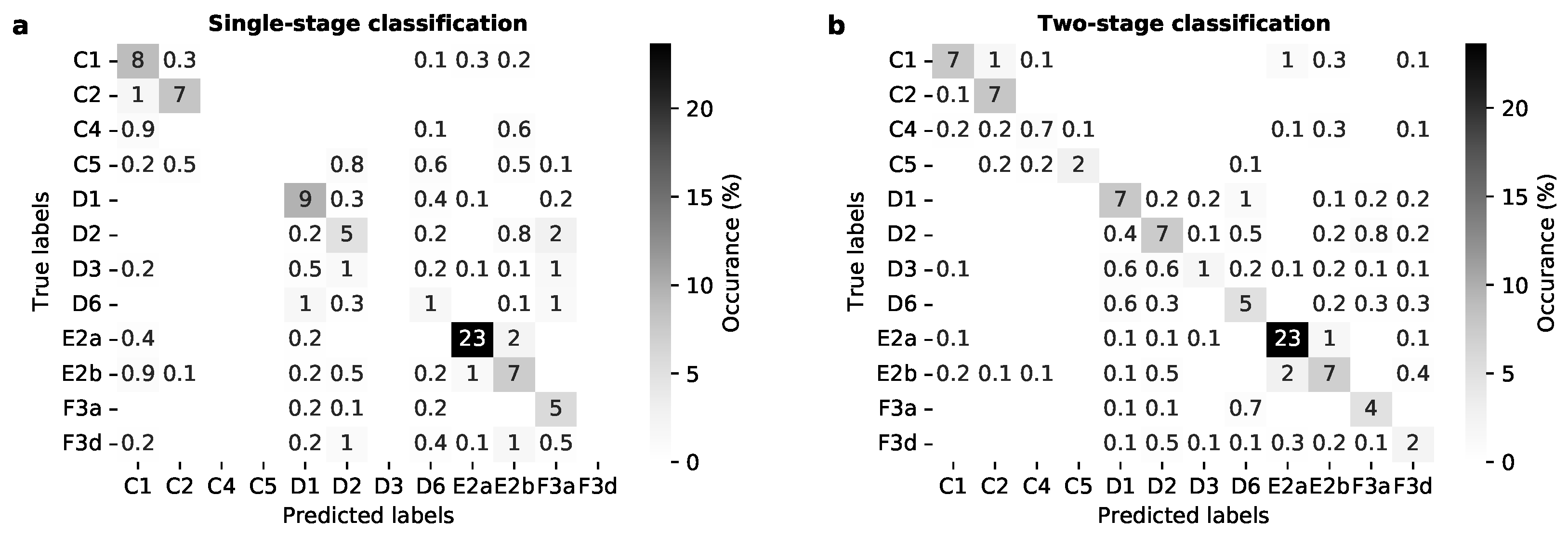
After evaluating the detailed classifiers individually, we then computed the effective accuracy of our multi-stage segmentation method (Table 6 and Figure 7). This takes into account instances for which the main classifier is incorrect, which subsequently leads to predictions from the wrong detailed classifier. As expected, precision and sensitivity are generally slightly lower for the effective accuracy (Table 6 vs. Table 5), but importantly, no single LC class dramatically decreased in performance. We then compared this performance to a naive, `single-stage’ classifier that was trained to predict the detailed classes directly from the aerial photography. Notably, this classifier was not able to learn the rare data classes (C4 scrub, C5 newly planted/felled trees, D3 bracken and F3d wet grassland and rush pasture) even though performance was similar for the more prevalent LC classes (Table 6 and Figure 7).

3.3. Land Cover Classification of PDNP

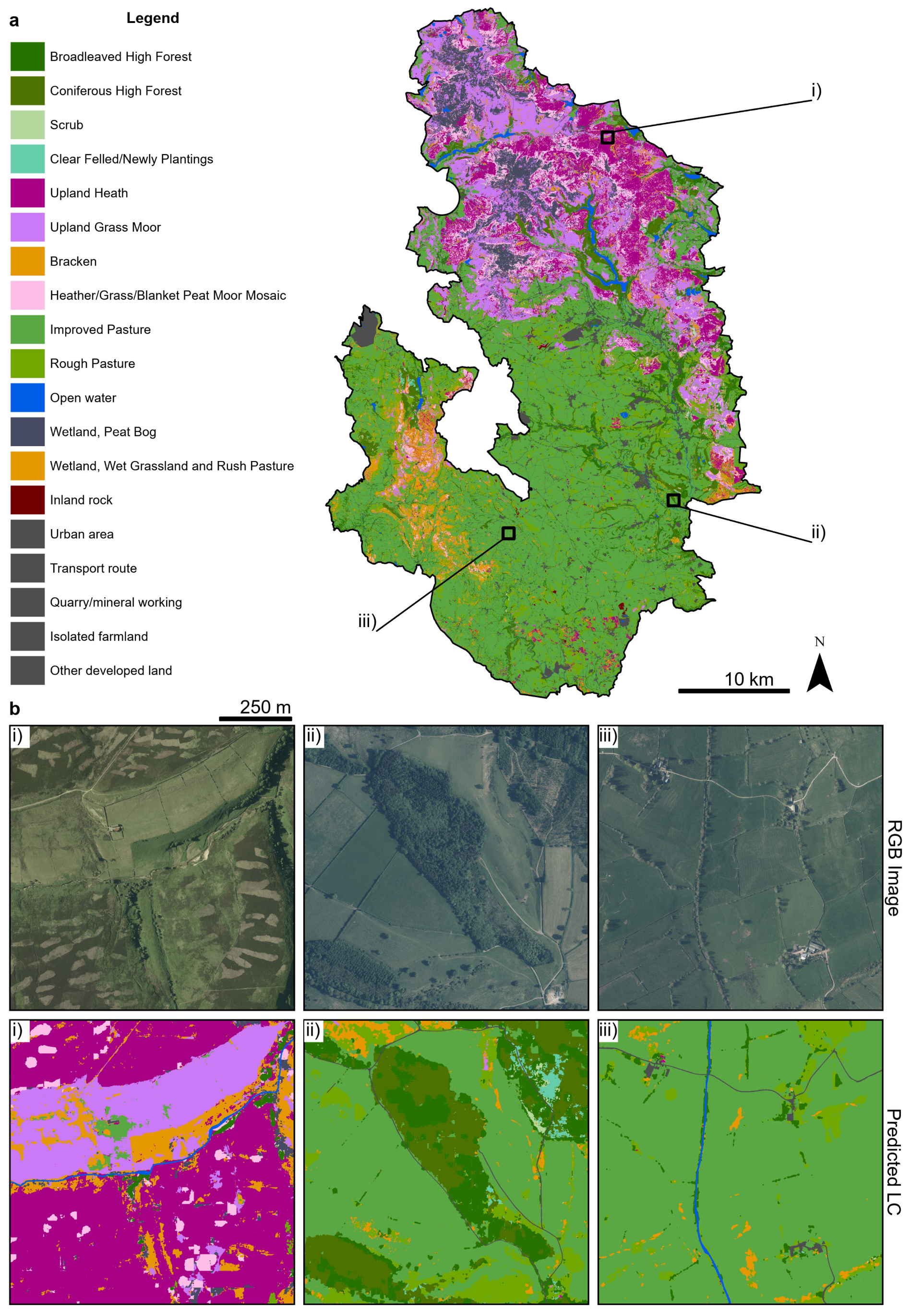
We next used our multi-stage approach to predict the land cover of the whole PDNP (Figure 8a). This LC map provides, to the best of our knowledge, the first very-high-(spatial)-resolution land cover map using the LC scheme designed for UK National Parks since 1991 [9,29]. Further, Figure 8 demonstrates the high resolution of predicted LC for three 1-km2 RGB image tiles.

3.4. Wet Grassland and Rush Pasture Habitat Fragmentation at a Landscape Scale

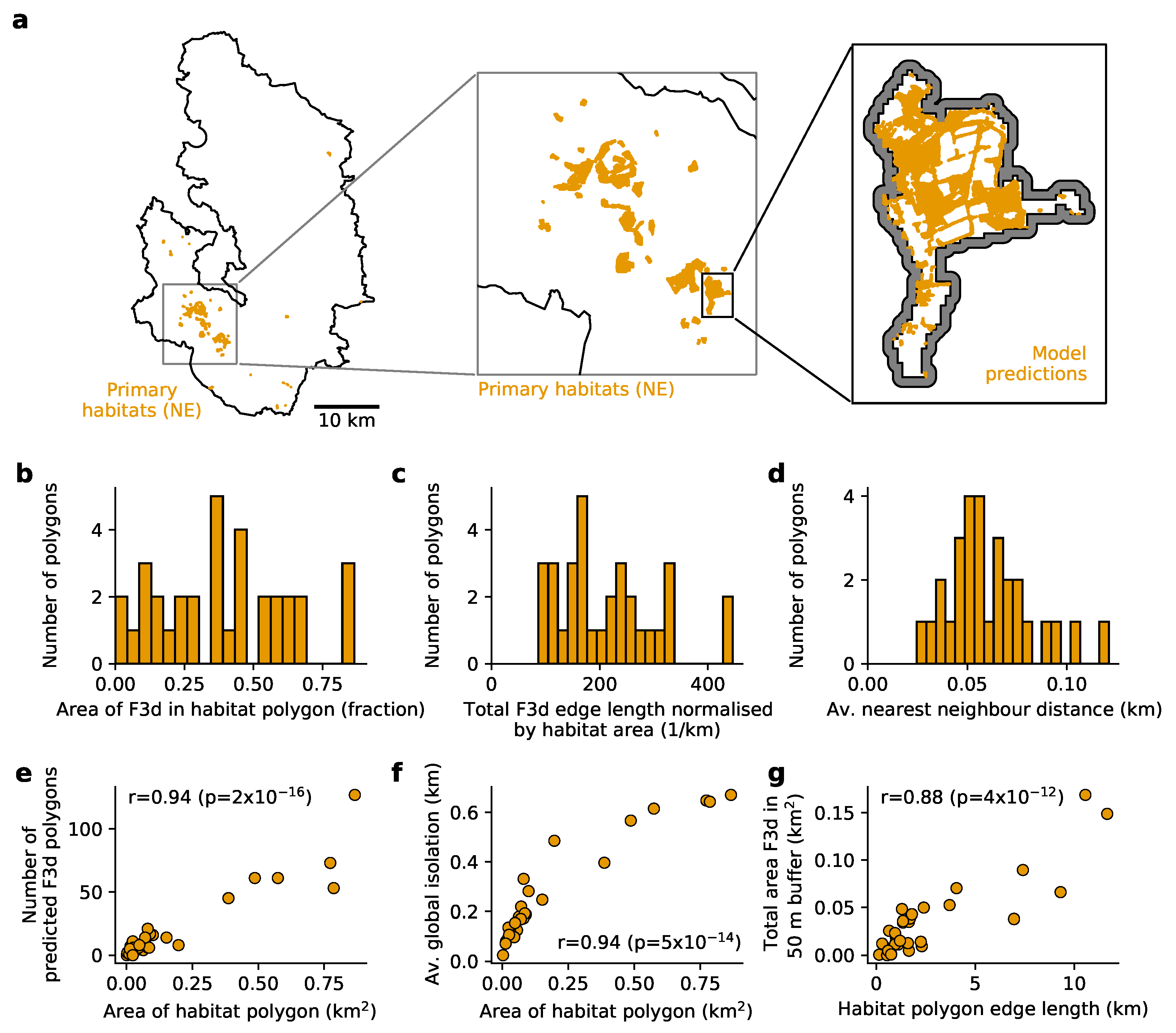
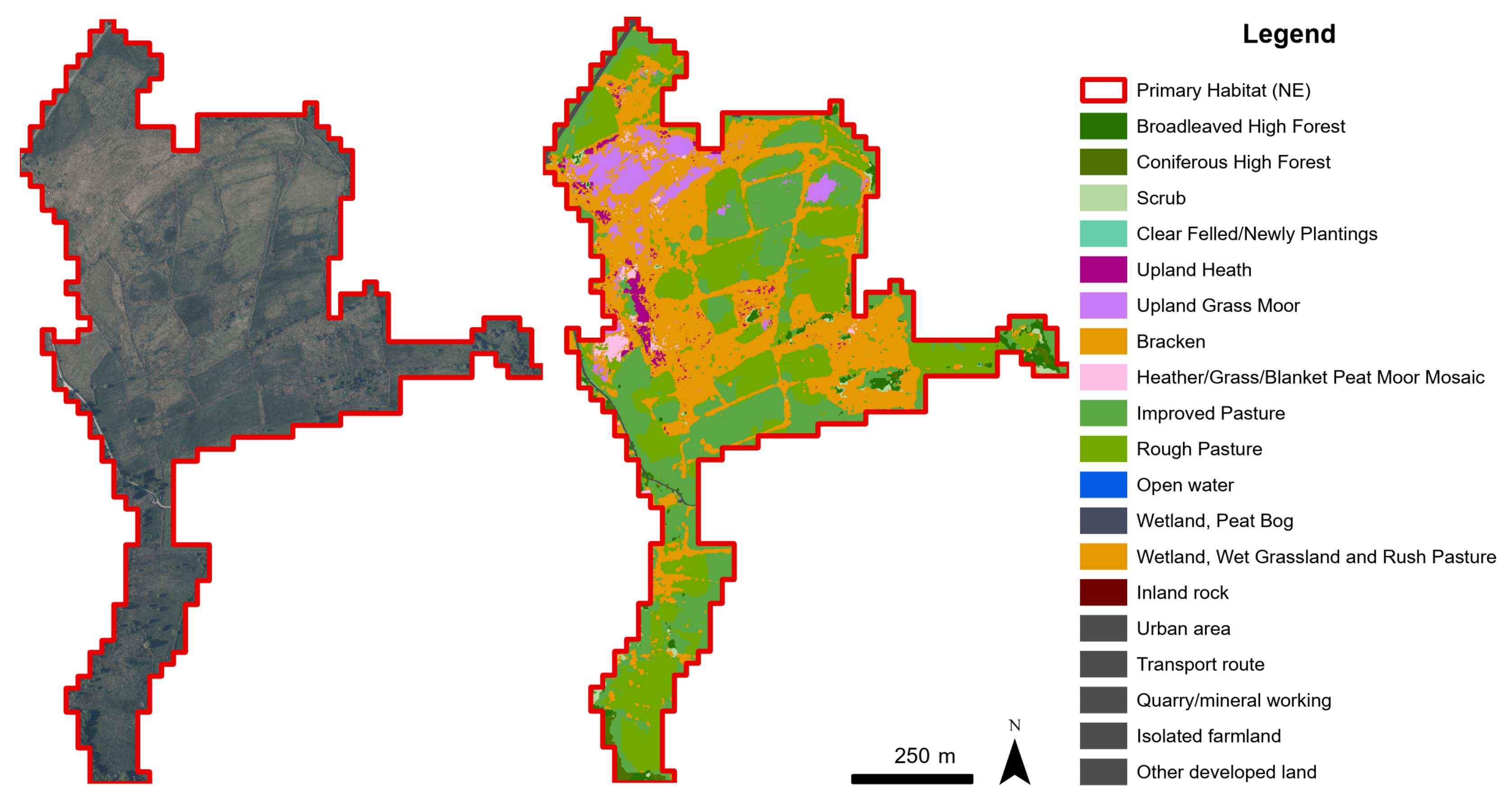
To demonstrate the added level of detail that our CNN predictions can provide, we analysed the extent of wet grassland and rush pasture (F3d) inside areas designated as `primary habitat’ (PH) of `purple moor grass & rush pasture’ by Natural England [44]. F3d PHs in the PDNP are concentrated at the South West Peak [32] (outlined in Figure 9a, middle panel), and therefore, we focused our analysis on that cluster of F3d habitats (Figure 9a and Figure 10). We predicted F3d using our developed CNN model in these places and analysed the spatial structure of F3d inside PH areas. We found that PHs varied in the number of F3d patches, F3d normalised edge length and F3d average nearest-neighbour distance (Figure 9b–d)—three metrics of habitat fragmentation [50,51]. We also identified spatial relationships that were consistent across PHs: larger PHs generally contained more F3d patches, with higher average global isolation among F3d patches (Figure 9e,f). Finally, PHs with longer edge lengths generally neighboured a higher area of F3d in their 50 m vicinity (Figure 9g).

4. Discussion

4.1. Multi-Stage Segmentation Approach

We developed a multi-stage approach for classifying hierarchical LC schemas with large variations in the density of each class. By deconstructing the classification process into multiple steps, we were able to achieve high accuracy on a large number of LC classes (95% accuracy on main classes, 92% on C, 72% on D and 87% on E; Table 3, Table 4 and Table 5).
A major advantage of the CNN is the minimal requirement for pre-processing of image data, as spatial patterns are more important than absolute spectral information for accurate prediction [18]. Still, differences in image timing can effect both training and inference because the appearance of LC classes can vary across seasons. We have not attempted to radiometrically balance images but have instead taken training samples from across the range of image dates (Figure 1) such that the model learns to recognise the LC classes despite variability in representations across imaging dates. We expect that further supervised training (fine-tuning) of the model will be necessary to predict LC from new aerial images where the date varies significantly from that of the training data.
The combination of very-high-resolution aerial photography, multi-stage training and a hierarchical LC schema led to predictions at a resolution of 12.5 cm, which marks a significant improvement over mapping products derived from satellite data [21]. This enables the identification of small habitat patches such as individual trees, wet grassland and rush pasture, heather patches and scrub (Figure 6 and Figure 8). This increase in resolution of habitat mapping can improve monitoring of fine-scale landscape features and enable classification schemas that contain more-detailed habitat types.
Our multi-stage approach to CNN training enabled the model to learn to recognise and predict minority LC classes that were not learned otherwise (Table 6). This is an important finding, as LC class density was highly variable at the landscape scale, leading to biased sample selection for CNN training and evaluation. The CNN training strategy developed here has the ability to detect specific habitat types or mixed ecotones within broad classes and homogeneous areas, which is important for biodiversity monitoring [52].

4.2. The Creation of a New LC Benchmark Data Set

We have created a data set of LC-annotated patches of RGB images that we have made publicly available online [42]. This also includes an interpretation key with image examples and written descriptions of all classes [38]. We have annotated over 1000 patches of size 64 m × 64 m at the level of the detailed LC schema, spanning over 20 LC classes (Table 1). Patches were sampled across the PDNP (Figure 1), which consequently led to variation in the flight dates (and associated variations in light conditions, seasonality effects on vegetation, time of day, etc.). This presented an additional challenge to the model and led to some misclassification because of spectral differences between some training and test data. This is an inherent challenge of large-scale applications of LC prediction, and we hope that by making our train and test data sets publicly available, this can further be addressed by the broader research community. Given the large number of classes, the focus on natural LC instead of urban LC, the spatial distribution and the variety both within and between classes, we believe that this data set is a valuable resource to the community and is representative of much of the upland landscape found in the UK.
The last complete census of LC in UK NPs was performed in the 1980s by manual interpretation of aerial photography [9]. Although human interpretation is generally considered to be the `gold standard’, annotating very large areas such as entire NPs (at 1:20,000 scale [9]) was found to be very resource-intensive and difficult [10]. Comparing aerial photography to ground observations, this census achieved 98% overall accuracy on main classes and 87% overall accuracy on subclasses using the same LC schema [10], which is only slightly better than our model predictions (95% accuracy on main classes and 72% to 92% accuracy on detailed classes).
In our study, given the much smaller quantity of manually annotated data compared to Taylor et al. [9], we were able to verify all manually annotated patches (used to train and evaluate the model) by a second, independent interpreter instead of quantifying the error based on a subsample of patches. We therefore did not quantify an annotation error, but instead, the second interpreter corrected the few instances where necessary. We were able to review all image patches (1027 patches of 64 m × 64 m) in detail, and field visits were conducted to resolve any remaining ambiguities.
Human annotation is, however, not the definite and only ground-truth. Boundaries between LC classes, when using one-hot encoding, are often ambiguous and can be drawn in various ways, which could all be considered correct by human interpreters. Therefore, when comparing model performance to human annotations, part of the error is caused by the one-sided evaluation that always favours human annotations over model predictions. To overcome this, a different evaluation strategy could be adopted whereby human interpreters are presented with model predictions and evaluate these without independent reference data. The main issues with this approach are, however, the obvious lack of reproducibility (by other researchers) and scalability, which together prevent efficient model optimisation and verification.

4.3. Land Cover Prediction of a UK National Park

In this study, we have demonstrated that Machine Learning LC annotation was able to efficiently scale to large areas; after training and testing on just over four square kilometres of LC image patches, we could predict the LC of 1439 km2 of land within days on a desktop computer (Figure 8). Compared to the visual interpretation approach [9,10] or low-resolution automated LC maps [21], our method facilitates a range of new applications that require detailed knowledge of the landscape’s land cover [53]. For example, these include fire risk modelling [8], climate change vulnerability assessments [4], tree planting planning [54], biodiversity monitoring [55,56] and habitat mapping [57,58,59].
Of particular interest are mosaics (of two classes) and other spatially heterogeneous habitats such as ecotones and ecolines. These habitats mark transitions between biological communities and are often seen as key to the biodiversity supported by an area [52]. However, collecting detailed information on habitat transitions to create spatially and temporally continuous data sets has historically been challenging [60]. Our methodology was able to identify landscape-scale persistent ecotones or ecolines (such as scrub or heather/grass mosaics), along with smaller-scale patch mosaic habitats, through the detection of the underlying ecotopes. This increased level of detail, combined with further geospatial analysis, could further drive new applications for LC maps.
Lastly, this technique could be used to update the high-resolution land cover census of all UK National Parks, as we have done for the PDNP, and researchers could begin to explore long-term LC changes alongside contemporary spatial data [61] that have occurred since Taylor et al. [9]. Scaling our approach across all UK landscapes (and, in particular, Protected Areas [27]) would improve the spatial resolution and detail of existing habitat monitoring. This could have wide implications, including accurate modelling of species distributions and movement and better-informed land management decisions for nature recovery and conservation.

4.4. Quantifying Fragmentation of Patch Habitats at a Landscape Scale

Recent studies have evidenced the importance of quantifying habitat fragmentation at the landscape scale [62,63,64]. Although low-resolution LC maps are sufficient for global habitat fragmentation analyses [51], local management and decision making require high-resolution maps of specific habitats. Our model was able to predict and quantify the fragmentation of patches of wet grassland and rush pasture (F3d) habitat within areas designated as primary habitat at 12.5 cm resolution (Figure 8).
Wet grassland and rush pasture is an important habitat, even in small patches, for a range of species including wetland birds, invertebrates, herpetofauna and small mammals if managed sympathetically [65,66]. Furthermore, this habitat has become increasingly present in marginal farmland as a result of the change of focus of farm subsidies and farming practices in the uplands over the last few decades [47]. Our objective was to leverage multi-stage semantic segmentation to accurately measure the extent of this habitat, not only as large vegetation stands but also as isolated patches within other primary vegetation classes and as common components of complex semi-natural vegetation mosaics [65]. We found that the spatial structure of wet grassland and rush pasture within these primary habitat areas showed substantial variation at fine scale (Figure 9b–d) using multiple habitat fragmentation indices [50,51]. At the same time, the CNN predictions revealed consistent spatial relationships that emerged across primary habitat areas (Figure 9e–g).
Major long-term environmental policies have set ambitious targets for conserving and restoring biodiversity [67,68,69]. There is growing evidence that small-scale (fragmented) habitats have the potential to support biodiversity when aggregated at a landscape scale [62,64]. However, coarse-scale LC maps limit the analysis and monitoring of these effects to the large-scale and, therefore, to high-level LC classes representing habitats [51]. We have demonstrated how CNNs can be used to quantify biodiversity by measuring habitats that occur at much smaller scales, such as wet grassland and rush pasture growing in gullies, scrub, heather/grass mosaics, rough pasture patches and bracken—all common vegetation types in the UK NPs [9]. Our method can be further applied to other regions using our publicly available code.
Finally, as the interest and demand for habitat corridors grows in the UK [67,70], detailed LC maps will be crucial to comprehend the extent and role of these mosaics and collections of fragmented habitat patches. In particular, a more-nuanced understanding of habitat mosaics and semi-natural fragments within highly managed areas may provide crucial opportunities for restoration connectivity and can facilitated by high-resolution LC maps.

5. Conclusions

We developed a multi-stage approach for classifying hierarchical LC schemes with large variations in the density of each class. Deconstructing the classification process into multiple steps achieved high accuracy on a large number of LC classes (95% accuracy on main classes, 92% on C, 72% on D and 87% on E), outperforming single-stage semantic segmentation for uneven class distributions. LC was predicted at high resolution (12.5 cm), enabling the identification of small habitat patches such as individual trees, heather patches and scrub. The multi-stage approach was also able to handle complex cosmopolitan habitats such as wet grassland and rush pasture, which occurs both within moorlands and grasslands, by including it in more than one detailed classifier.
Our approach can be used to detect a wide range of habitats from the same aerial image data: from those with a broad species mix and mosaics to single species. This has wide-ranging applications in landscape ecology and biodiversity monitoring, especially in regions where important habitats are small and mixed. This work helps to overcome the current limitations in spatial resolution and habitat detail for understanding species movement and distributions and measuring progress against nature recovery targets, such as those set out in the UK’s “25 Year Environment Plan” and the UN’s “Sustainability Goals”.

Author Contributions

T.L.v.d.P. performed the data analysis and wrote the first manuscript draft. T.L.v.d.P. and D.G.A. performed the data visualisation. S.T.G. and D.G.A. created the annotated LC data set. D.M.S. and D.G.A. conceived and supervised the project. All authors contributed to writing and editing of the manuscript. All authors have read and agreed to the published version of the manuscript.

Funding

T.L.v.d.P. was supported by funding from the Biotechnology and Biological Sciences Research Council (BBSRC), grant number BB/M011224/1. This research was supported by funding from The Alan Turing Institute via the internship scheme Turing Internship Network, and by the Peak District National Park Authority.

Data Availability Statement

Data supporting this study (train and test data set of RGB images and land cover annotations) are openly available from the Cranfield Online Research Data (CORD) repository at https://doi.org/10.17862/cranfield.rd.24221314.

Conflicts of Interest

The authors declare no competing interests. The views expressed in this study are those of the authors and are not necessarily those of the Peak District National Park Authority.

References

  1. Szantoi, Z.; Geller, G.N.; Tsendbazar, N.E.; See, L.; Griffiths, P.; Fritz, S.; Gong, P.; Herold, M.; Mora, B.; Obregón, A. Addressing the need for improved land cover map products for policy support. Environ. Sci. Policy 2020, 112, 28–35. [Google Scholar] [CrossRef] [PubMed]
  2. Crowley, M.A.; Cardille, J.A. Remote sensing’s recent and future contributions to landscape ecology. Curr. Landsc. Ecol. Rep. 2020, 5, 45–57. [Google Scholar] [CrossRef]
  3. Halim, M.; Ahmad, A.; Rahman, M.; Amin, Z.; Khanan, M.; Musliman, I.; Kadir, W.; Jamal, M.; Maimunah, D.; Wahab, A.; et al. Land use/land cover mapping for conservation of UNESCO Global Geopark using object and pixel-based approaches. In The IOP Conference Series: Earth and Environmental Science; IOP Publishing: Bristol, UK, 2018; Volume 169, p. 012075. [Google Scholar]
  4. Santos, M.J.; Smith, A.B.; Dekker, S.C.; Eppinga, M.B.; Leitão, P.J.; Moreno-Mateos, D.; Morueta-Holme, N.; Ruggeri, M. The role of land use and land cover change in climate change vulnerability assessments of biodiversity: A systematic review. Landsc. Ecol. 2021, 36, 3367–3382. [Google Scholar] [CrossRef]
  5. Roy, P.S.; Ramachandran, R.M.; Paul, O.; Thakur, P.K.; Ravan, S.; Behera, M.D.; Sarangi, C.; Kanawade, V.P. Anthropogenic land use and land cover changes—A review on its environmental consequences and climate change. J. Indian Soc. Remote Sens. 2022, 50, 1615–1640. [Google Scholar] [CrossRef]
  6. Rayner, M.; Balzter, H.; Jones, L.; Whelan, M.; Stoate, C. Effects of improved land-cover mapping on predicted ecosystem service outcomes in a lowland river catchment. Ecol. Indic. 2021, 133, 108463. [Google Scholar] [CrossRef]
  7. Burke, T.; Whyatt, J.D.; Rowland, C.; Blackburn, G.A.; Abbatt, J. The influence of land cover data on farm-scale valuations of natural capital. Ecosyst. Serv. 2020, 42, 101065. [Google Scholar] [CrossRef]
  8. Millin-Chalabi, G.; Labenski, P.; Pascagaza, A.M.P.; Clay, G.; Fassnacht, F.E. Dynamic fuel mapping in the South Pennines using a multitemporal intensity and coherence approach. In Proceedings of the European Space Agency-Fringe 2023, Leeds, UK, 11–15 September 2023. [Google Scholar]
  9. Taylor, J.; Bird, A.C.; Keech, M.; Stuttard, M. Landscape Change in the National Parks of England and Wales: Final Report, Volume I Main Report; Silsoe College: Bedford, UK, 1991; Available online: https://publications.naturalengland.org.uk/publication/5216333889273856 (accessed on 5 November 2023.).
  10. Taylor, J.C.; Brewer, T.R.; Bird, A.C. Monitoring landscape change in the National Parks of England and Wales using aerial photo interpretation and GIS. Int. J. Remote Sens. 2000, 21, 2737–2752. [Google Scholar] [CrossRef]
  11. Maxwell, A.E.; Strager, M.P.; Warner, T.A.; Ramezan, C.A.; Morgan, A.N.; Pauley, C.E. Large-area, high spatial resolution land cover mapping using random forests, GEOBIA, and NAIP orthophotography: Findings and recommendations. Remote Sens. 2019, 11, 1409. [Google Scholar] [CrossRef]
  12. Witjes, M.; Parente, L.; van Diemen, C.J.; Hengl, T.; Landa, M.; Brodský, L.; Halounova, L.; Križan, J.; Antonić, L.; Ilie, C.M.; et al. A spatiotemporal ensemble machine learning framework for generating land use/land cover time-series maps for Europe (2000–2019) based on LUCAS, CORINE and GLAD Landsat. PeerJ 2022, 10, e13573. [Google Scholar] [CrossRef]
  13. Bradter, U.; Thom, T.J.; Altringham, J.D.; Kunin, W.E.; Benton, T.G. Prediction of National Vegetation Classification communities in the British uplands using environmental data at multiple spatial scales, aerial images and the classifier random forest. J. Appl. Ecol. 2011, 48, 1057–1065. [Google Scholar] [CrossRef]
  14. Kattenborn, T.; Leitloff, J.; Schiefer, F.; Hinz, S. Review on Convolutional Neural Networks (CNN) in vegetation remote sensing. ISPRS J. Photogramm. Remote Sens. 2021, 173, 24–49. [Google Scholar] [CrossRef]
  15. García-Álvarez, D.; Nanu, S.F. Land Use Cover Datasets: A Review. In Land Use Cover Datasets and Validation Tools; Springer Nature: Cham, Switzerland, 2022; p. 47. [Google Scholar]
  16. Faccioli, M.; Zonneveld, S.; Tyler, C.R.; Day, B. Does local Natural Capital Accounting deliver useful policy and management information? A case study of Dartmoor and Exmoor National Parks. J. Environ. Manag. 2023, 327, 116272. [Google Scholar] [CrossRef] [PubMed]
  17. Horning, N. Land cover mapping with ultra-high-resolution aerial imagery. Remote Sens. Ecol. Conserv. 2020, 6, 429–430. [Google Scholar] [CrossRef]
  18. Kattenborn, T.; Eichel, J.; Wiser, S.; Burrows, L.; Fassnacht, F.E.; Schmidtlein, S. Convolutional Neural Networks accurately predict cover fractions of plant species and communities in Unmanned Aerial Vehicle imagery. Remote Sens. Ecol. Conserv. 2020, 6, 472–486. [Google Scholar] [CrossRef]
  19. Horning, N.; Fleishman, E.; Ersts, P.J.; Fogarty, F.A.; Wohlfeil Zillig, M. Mapping of land cover with open-source software and ultra-high-resolution imagery acquired with unmanned aerial vehicles. Remote Sens. Ecol. Conserv. 2020, 6, 487–497. [Google Scholar] [CrossRef]
  20. Clutterbuck, B.; Yallop, A.; Thacker, J. Monitoring the Impact of Blanket Bog Conservation in the South Pennine Moors Special Area of Conservation Using an Unmanned Aerial Vehicle; Nottingham Trent University & CS Conservation Survey: Notthingham, UK, 2021. [Google Scholar]
  21. García-Álvarez, D.; Lara Hinojosa, J.; Jurado Pérez, F.J.; Quintero Villaraso, J. General Land Use Cover Datasets for Europe. In Land Use Cover Datasets and Validation Tools: Validation Practices with QGIS; Springer International Publishing: Cham, Switzerland, 2022; pp. 313–345. [Google Scholar]
  22. Sertel, E.; Topaloğlu, R.H.; Şallı, B.; Yay Algan, I.; Aksu, G.A. Comparison of landscape metrics for three different level land cover/land use maps. ISPRS Int. J. Geo-Inf. 2018, 7, 408. [Google Scholar] [CrossRef]
  23. Marston, C.; Rowland, C.; O’Neil, A.; Morton, R. Land Cover Map 2021 (10 m classified pixels, GB). NERC EDS Environmental Information Data Centre. 2022. Available online: https://catalogue.ceh.ac.uk/documents/a22baa7c-5809-4a02-87e0-3cf87d4e223a (accessed on 6 November 2023).
  24. Kilcoyne, A.; Clement, M.; Moore, C.; Picton Phillipps, G.; Keane, R.; Woodget, A.; Potter, S.; Stefaniak, A.; Trippier, B. Living England: Satellite-Based Habitat Classification. Technical User Guide. 2022. Available online: http://nepubprod.appspot.com/publication/4918342350798848 (accessed on 11 November 2022).
  25. Tulbure, M.G.; Hostert, P.; Kuemmerle, T.; Broich, M. Regional matters: On the usefulness of regional land-cover datasets in times of global change. Remote Sens. Ecol. Conserv. 2022, 8, 272–283. [Google Scholar] [CrossRef]
  26. Dudley, N. Guidelines for Applying Protected Area Management Categories; IUCN: Gland, Switzerland, 2008. [Google Scholar]
  27. Starnes, T.; Beresford, A.E.; Buchanan, G.M.; Lewis, M.; Hughes, A.; Gregory, R.D. The extent and effectiveness of protected areas in the UK. Glob. Ecol. Conserv. 2021, 30, e01745. [Google Scholar] [CrossRef]
  28. Ahern, K.; Cole, L. Landscape scale–towards an integrated approach. Ecos 2012, 33, 6–12. [Google Scholar]
  29. Taylor, J.; Bird, A.C.; Brewer, T.; Keech, M.; Stuttard, M. Landscape Change in the National Parks of England and Wales: Final Report, Volume II Methodology; Silsoe College: Bedford, UK, 1991. [Google Scholar]
  30. Bluesky. Aerial Photography for Great Britain ©; Bluesky International Limited and Getmapping Plc.: Ashby-De-La-Zouch, UK, 2022; Available online: https://apgb.blueskymapshop.com/ (accessed on 6 November 2023).
  31. Ordnance Survey. OS National Geographic Database ©; Ordnance Survey: Southampton, UK, 2023; Available online: https://beta.ordnancesurvey.co.uk/products/os-ngd-api-features (accessed on 6 November 2023).
  32. Natural England. National Character Area Profiles. 2014. Available online: https://www.gov.uk/government/publications/national-character-area-profiles-data-for-local-decision-making/national-character-area-profiles (accessed on 27 September 2023).
  33. Brodrick, P.G.; Davies, A.B.; Asner, G.P. Uncovering ecological patterns with convolutional neural networks. Trends Ecol. Evol. 2019, 34, 734–745. [Google Scholar] [CrossRef]
  34. Ronneberger, O.; Fischer, P.; Brox, T. U-net: Convolutional networks for biomedical image segmentation. In Proceedings of the Medical Image Computing and Computer-Assisted Intervention–MICCAI 2015: 18th International Conference, Munich, Germany, 5–9 October 2015; Proceedings, Part III 18. Springer: New York, NY, USA, 2015; pp. 234–241. [Google Scholar]
  35. Simms, D.M. Fully convolutional neural nets in-the-wild. Remote Sens. Lett. 2020, 11, 1080–1089. [Google Scholar] [CrossRef]
  36. Lobo Torres, D.; Queiroz Feitosa, R.; Nigri Happ, P.; Elena Cué La Rosa, L.; Marcato Junior, J.; Martins, J.; Olã Bressan, P.; Gonçalves, W.N.; Liesenberg, V. Applying fully convolutional architectures for semantic segmentation of a single tree species in urban environment on high resolution UAV optical imagery. Sensors 2020, 20, 563. [Google Scholar] [CrossRef]
  37. Iakubovskii, P. Segmentation Models Pytorch. 2019. Available online: https://github.com/qubvel/segmentation_models.pytorch (accessed on 6 November 2023).
  38. Alexander, D.G.; Van der Plas, T.L.; Geikie, S.T. Interpretation Key of Peak District Land Cover Classes. 2023. Available online: https://reports.peakdistrict.gov.uk/interpretation-key/docs/introduction.html (accessed on 27 September 2023).
  39. Rodwell, J.S. British Plant Communities; Cambridge University Press: Cambridge, UK, 1998; Volume 2. [Google Scholar]
  40. Alderson, D.M.; Evans, M.G.; Shuttleworth, E.L.; Pilkington, M.; Spencer, T.; Walker, J.; Allott, T.E. Trajectories of ecosystem change in restored blanket peatlands. Sci. Total Environ. 2019, 665, 785–796. [Google Scholar] [CrossRef] [PubMed]
  41. Maxwell, A.E.; Warner, T.A.; Guillén, L.A. Accuracy assessment in convolutional neural network-based deep learning remote sensing studies—Part 2: Recommendations and best practices. Remote Sens. 2021, 13, 2591. [Google Scholar] [CrossRef]
  42. Van der Plas, T.L.; Geikie, S.T.; Alexander, D.G.; Simms, D.M. Very High Resolution Aerial Photography and Annotated Land Cover Data of the Peak District [Dataset]. 2023. Available online: https://cord.cranfield.ac.uk/articles/dataset/Very_high_resolution_aerial_photography_and_annotated_land_cover_data_of_the_Peak_District_National_Park/24221314 (accessed on 9 October 2023).
  43. Forestry Commission. National Forest Inventory Woodland GB 2020; Forestry Commission Open Data Publication, Last Updated 30 June 2022; Forestry Commission: Bristol, UK, 2022. Available online: https://data-forestry.opendata.arcgis.com/datasets/eb05bd0be3b449459b9ad0692a8fc203_0/about (accessed on 6 November 2023).
  44. Natural England. Habitat Networks (England)—Purple Moor Grass & Rush Pasture; Natural England Open Data Publication, Last Updated 5 April 2022; Natural England: UK, 2022; Available online: https://naturalengland-defra.opendata.arcgis.com/datasets/Defra::habitat-networks-england-purple-moor-grass-rush-pasture (accessed on 6 November 2023).
  45. Natural England. Peaty Soils Location (England). 2022. Available online: https://naturalengland-defra.opendata.arcgis.com/datasets/1e5a1cdb2ab64b1a94852fb982c42b52_0/about (accessed on 27 September 2023).
  46. Stace, C. New Flora of the British Isles; Cambridge University Press: Cambridge, UK, 2010. [Google Scholar]
  47. Ashby, M.A.; Whyatt, J.D.; Rogers, K.; Marrs, R.H.; Stevens, C.J. Quantifying the recent expansion of native invasive rush species in a UK upland environment. Ann. Appl. Biol. 2020, 177, 243–255. [Google Scholar] [CrossRef]
  48. Paszke, A.; Gross, S.; Massa, F.; Lerer, A.; Bradbury, J.; Chanan, G.; Killeen, T.; Lin, Z.; Gimelshein, N.; Antiga, L.; et al. Pytorch: An imperative style, high-performance deep learning library. In Advances in Neural Information Processing Systems; NeurIPS: Vancouver, BC, Canada, 2019; Volume 32. [Google Scholar]
  49. Hunter, J.D. Matplotlib: A 2D graphics environment. Comput. Sci. Eng. 2007, 9, 90–95. [Google Scholar] [CrossRef]
  50. Wang, X.; Blanchet, F.G.; Koper, N. Measuring habitat fragmentation: An evaluation of landscape pattern metrics. Methods Ecol. Evol. 2014, 5, 634–646. [Google Scholar] [CrossRef]
  51. Watling, J.I.; Arroyo-Rodríguez, V.; Pfeifer, M.; Baeten, L.; Banks-Leite, C.; Cisneros, L.M.; Fang, R.; Hamel-Leigue, A.C.; Lachat, T.; Leal, I.R.; et al. Support for the habitat amount hypothesis from a global synthesis of species density studies. Ecol. Lett. 2020, 23, 674–681. [Google Scholar] [CrossRef]
  52. Loke, L.H.; Chisholm, R.A. Measuring habitat complexity and spatial heterogeneity in ecology. Ecol. Lett. 2022, 25, 2269–2288. [Google Scholar] [CrossRef]
  53. Gatis, N.; Carless, D.; Luscombe, D.J.; Brazier, R.E.; Anderson, K. An operational land cover and land cover change toolbox: Processing open-source data with open-source software. Ecol. Solut. Evid. 2022, 3, e12162. [Google Scholar] [CrossRef]
  54. Peak District National Park Authority. The Wooded Landscapes Plan: Increasing Tree and Scrub Cover in the Peak District National Park Landscapes (2022–2032). 2022. Available online: https://www.peakdistrict.gov.uk/__data/assets/pdf_file/0027/447255/Wooded-Landscapes-Plan-Final-Draft-July-22.pdf (accessed on 27 September 2023).
  55. Tuia, D.; Kellenberger, B.; Beery, S.; Costelloe, B.R.; Zuffi, S.; Risse, B.; Mathis, A.; Mathis, M.W.; van Langevelde, F.; Burghardt, T.; et al. Perspectives in machine learning for wildlife conservation. Nat. Commun. 2022, 13, 792. [Google Scholar] [CrossRef] [PubMed]
  56. Rolnick, D.; Donti, P.L.; Kaack, L.H.; Kochanski, K.; Lacoste, A.; Sankaran, K.; Ross, A.S.; Milojevic-Dupont, N.; Jaques, N.; Waldman-Brown, A.; et al. Tackling climate change with machine learning. ACM Comput. Surv. (CSUR) 2022, 55, 1–96. [Google Scholar] [CrossRef]
  57. O’Connell, J.; Bradter, U.; Benton, T.G. Wide-area mapping of small-scale features in agricultural landscapes using airborne remote sensing. ISPRS J. Photogramm. Remote Sens. 2015, 109, 165–177. [Google Scholar] [CrossRef] [PubMed]
  58. Bhatt, P.; Maclean, A.; Dickinson, Y.; Kumar, C. Fine-Scale Mapping of Natural Ecological Communities Using Machine Learning Approaches. Remote Sens. 2022, 14, 563. [Google Scholar] [CrossRef]
  59. Kubacka, M.; Żywica, P.; Subirós, J.V.; Bródka, S.; Macias, A. How do the surrounding areas of national parks work in the context of landscape fragmentation? A case study of 159 protected areas selected in 11 EU countries. Land Use Policy 2022, 113, 105910. [Google Scholar] [CrossRef]
  60. D’Urban Jackson, T.; Williams, G.J.; Walker-Springett, G.; Davies, A.J. Three-dimensional digital mapping of ecosystems: A new era in spatial ecology. Proc. R. Soc. B 2020, 287, 20192383. [Google Scholar] [CrossRef]
  61. Ridding, L.E.; Watson, S.C.; Newton, A.C.; Rowland, C.S.; Bullock, J.M. Ongoing, but slowing, habitat loss in a rural landscape over 85 years. Landsc. Ecol. 2020, 35, 257–273. [Google Scholar] [CrossRef]
  62. Fahrig, L. Ecological responses to habitat fragmentation per se. Annu. Rev. Ecol. Evol. Syst. 2017, 48, 1–23. [Google Scholar] [CrossRef]
  63. Chase, J.M.; Blowes, S.A.; Knight, T.M.; Gerstner, K.; May, F. Ecosystem decay exacerbates biodiversity loss with habitat loss. Nature 2020, 584, 238–243. [Google Scholar] [CrossRef]
  64. Riva, F.; Fahrig, L. Landscape-scale habitat fragmentation is positively related to biodiversity, despite patch-scale ecosystem decay. Ecol. Lett. 2023, 26, 268–277. [Google Scholar] [CrossRef]
  65. Natural England; RSPB. Climate Change Adaptation Manual—Evidence to Support Nature Conservation in a Changing Climate, 2nd ed.; Natural England: York, UK, 2019. [Google Scholar]
  66. Kelly, L.; Douglas, D.; Shurmer, M.; Evans, K. Upland rush management advocated by agri-environment schemes increases predation of artificial wader nests. Anim. Conserv. 2021, 24, 646–658. [Google Scholar] [CrossRef]
  67. UK Department for Environment, Food & Rural Affairs. A Green Future: Our 25 Year Plan to Improve the Environment. 2018. Available online: https://www.gov.uk/government/publications/25-year-environment-plan (accessed on 27 September 2023).
  68. United Nations Environment Programme. UN Biodiversity Conference (COP 15). 2022. Available online: https://www.unep.org/un-biodiversity-conference-cop-15 (accessed on 27 September 2023).
  69. Department for Environment, Food and Rural Affairs. Environmental Land Management Update: How Government Will Pay for Land-Based Environment and Climate Goods and Services. 2023. Available online: https://www.gov.uk/government/publications/environmental-land-management-update-how-government-will-pay-for-land-based-environment-and-climate-goods-and-services (accessed on 27 September 2023).
  70. Bailey, J.J.; Cunningham, C.A.; Griffin, D.C.; Hoppit, G.; Metcalfe, C.A.; Schéré, C.M.; Travers, T.J.P.; Turner, R.K.; Hill, J.K.; Sinnadurai, P.; et al. Protected Areas and Nature Recovery. Achieving the Goal to Protect 30% of UK Land and Seas for Nature by 2030; British Ecological Society: London, UK, 2022. [Google Scholar]
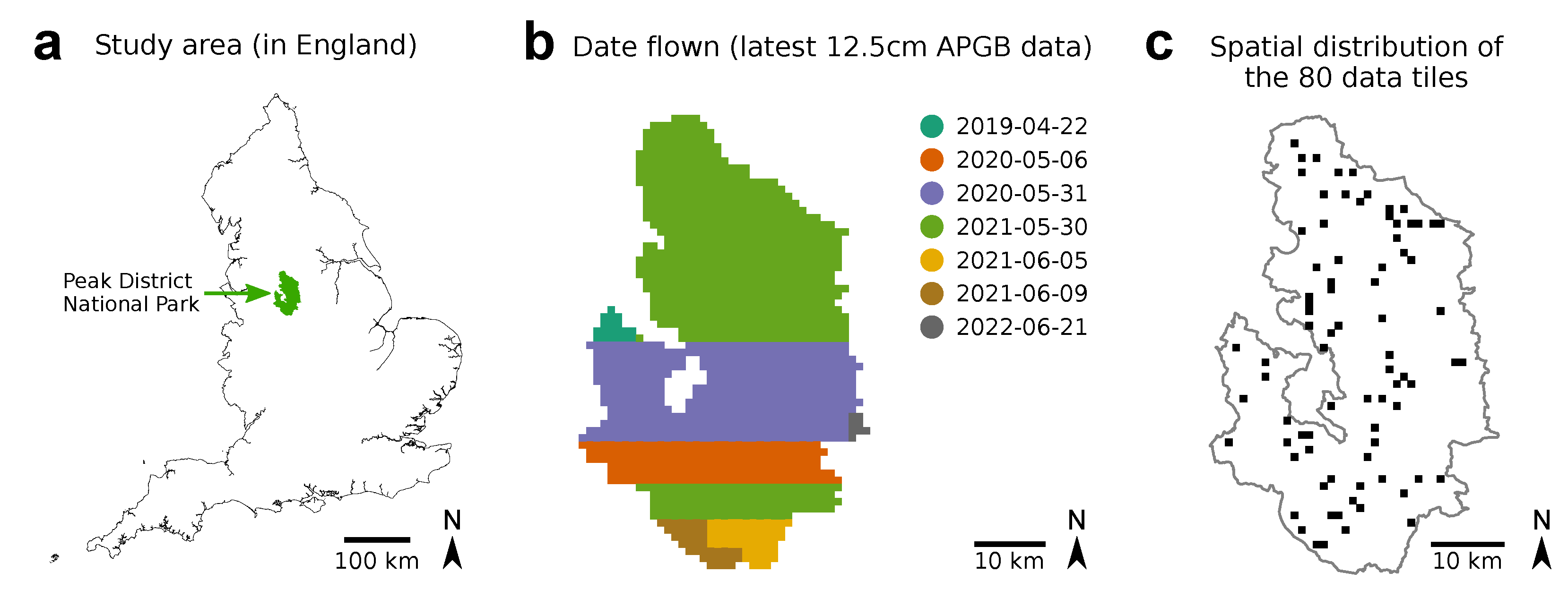
Figure 1. Study area details. (a) Our area of study is the Peak District National Park, outlined in green (within England). (b) RGB image capture date per square kilometre tile, determined from APGB metadata (of latest 12.5 cm RGB data) [30]. (c) Distribution of 80 tiles used to create image patch data set. Each square tile is of size 1 km2.
Remotesensing 15 05277 g001
Figure 2. Multi-stage semantic segmentation approach, where (a) land cover (LC) is predicted from RGB images in multiple stages: classification of the main class, overlaying the OS NGD layer, classification of the detailed subclasses, and post-processing to further split up subclasses (based on soil data). (b) The classifiers are Convolutional Neural Networks that use the U-Net architecture, consisting of convolutional layers as well as skip connections [14,34] to map RGB images to LC predictions. (c) The LC schema is hierarchical, and multiple classifiers and post-processing layers are used to predict all subclasses. Colours correspond to the steps in panel (a). LC codes are explained in Table 1.
Remotesensing 15 05277 g002
Figure 3. Distribution of evaluation tiles. Left: the PDNP outline and the first set of fifty 1-km 2 square tiles for evaluation. Right: The density of each LC class, calculated using the LC80 data, for the set of 50 evaluation tiles (x-axis) and the entire PDNP (y-axis). The LC codes are described in Table 1.
Remotesensing 15 05277 g003
Figure 4. Efficientnet predictions strongly followed the image patch grid structure. RGB image overlayed with E2b (rough pasture) predictions in blue. The best E-classifier Resnet was compared to the best E-classifier Efficientnet (in terms of minimising the test loss).
Remotesensing 15 05277 g004
Figure 5. Semantic segmentation of main classes. (a) Main class classifiers converged, as demonstrated by the test data loss (while convergence was determined based on training loss). (b) Distribution of data per main class, where the train and test data consisted of 70% and 30% of the data, respectively. The right y-axis indicates the equivalent number of full 64 m × 64 m patches (i.e., the total area per class divided by the area per patch). (c) Confusion matrix of the model’s predictions on the test data. This is further quantified in Table 4. (d) Five example images (top) and their predicted land cover (bottom) are shown; the size is that which was presented to the CNN model (64 m × 64 m, North-oriented). C—woodlands, D—moorlands and E—grasslands.
Remotesensing 15 05277 g005
Figure 6. Semantic segmentation of detailed classes. (a) Detailed class classifiers converged, as demonstrated by their test data loss (normalised by loss at first epoch). (b) Distribution of data per detailed class, where the train and test data consisted of 70% and 30% of the data, respectively. (c) Confusion matrix of the model’s predictions on the test data. This is further quantified in Table 5. The x-axis and y-axis are coloured according to the classifier that was trained to predict the classes (also see Figure 2c). (d) Three example images (left) and their predicted land cover (right) are shown, one for each of the three subclass classifiers. (e) A further five example images are shown, demonstrating the final predictions by using the main class predictions as a mask for applying the combination of detailed class classifiers (also see Figure 2a). LC codes are explained in Table 1.
Remotesensing 15 05277 g006
Figure 7. Confusion matrices for single-stage and multi-stage classifiers (evaluated on the test data): (a) The single-stage classifier predicted all detailed classes directly from the RGB data. Five CNNs were trained, and the best-performing model was chosen. The single-stage model was not able to learn to classify C4, C5, D3 and F3d—four relatively rare classes. (b) Results for the multi-stage classifier. Results are shown before post-processing and without the OS layer (i.e., just the detailed class CNN predictions). The effective fractions are shown, i.e., after both the main and detailed classifiers have been applied. See also Table 6.
Remotesensing 15 05277 g007
Figure 8. (a) Detailed land cover predictions for entire Peak District National Park (1439 km2). (b) Close-ups of the three insets shown in panel (a). The RGB images (top) and model predictions (bottom) of three 1 km × 1 km example tiles are shown.
Remotesensing 15 05277 g008
Figure 9. Analysis of wet grassland and rush pasture extent in the South West Peak. (a) Left and middle panels: PDNP outline (black) and F3d primary habitat (PH) polygons from Natural England [44] (orange). Right: close-up of one PH polygon (black) with a 50 m buffer zone (grey) overlaid with CNN predictions of F3d (orange). Only PHs inside the square box of the left and middle panel were analysed. Also see Figure 10. (b) Fraction of F3d-predicted area per PH polygon. (c) Total edge length of all F3d-predicted areas within PH polygons, normalised by PH polygon area. (d) Average nearest-neighbour distance between F3d-predicted areas within each PH polygon (with at least 2 F3d-predicted areas). (e) PH area vs. number of F3d-predicted polygons. Pearson correlation r and p value p are stated in the panel. (f) PH area vs. average global isolation (i.e., mean distance from focal F3d-polygon to all other F3d-polygons) across F3d-predicted polygons inside PH. (g) PH edge length vs. total F3d area inside PH buffer zone (i.e., excluding PH itself).
Remotesensing 15 05277 g009
Figure 10. RGB image (left) and LC predictions (right) for the example area of Primary Habitat designated by the Habitat Networks (England)—Purple Moor Grass & Rush Pasture Natural England (also see Figure 9a).
Remotesensing 15 05277 g010
Table 2. Overview of external GIS data sets used. “Used for”: refers to to either Training, Testing, Prediction or Analysis. NFI data contain Forestry Commission information licensed under the Open Government License v3.0. © Crown copyright and database right 2020 Ordnance Survey [100021242].
NameDescriptionSourceUsed forTotal Area Used
National Forest Inventory (NFI) woodland mapWoodlands with an area over 0.5 ha with a minimum of 20% canopy cover and a minimum width of 20 m. Woodlands are classified similarly to C1–C5 in our LC schema.Forestry Commission [43]Training, testing4.2 km2
OS NGD dataTopographical layer of developed land and waterways. Classes were aggregated to connect to our LC schema (F2, G2a and H classes).Ordnance Survey © [31]Testing, prediction1439 km2
Habitat Networks (England)—Purple Moor Grass & Rush PastureMap of UK habitatsNatural England Open Data Publication [44]Analysis1439 km2
Peaty Soils Location (England)Soil contentNatural England Open Data Publication, BGS, Cranfield University (NSRI) and OS [45]Prediction1439 km2
Table 3. Average CNN performance. The loss function was varied for each of the four classifiers (main, C, D and E). Five runs were performed for each model for 60 epochs; the model with the best results (in terms of training loss) was saved. Afterwards, the mean, standard deviation (std) and maximum (max) accuracy on test data were computed for each classifier. Focal loss was used with γ = 0.75 . The `Selected?’ column indicates whether the maximum-performing model of that classifier type was used in further analyses. Additionally, five runs were performed for the single-stage model, which learns to classify the detailed classes directly using the cross entropy loss function.
ClassifierLoss FunctionMeanStdMaxSelected?
CCross entropy0.900.010.92Yes
CFocal loss0.870.100.93-
DCross entropy0.670.030.72Yes
DFocal loss0.700.020.72-
ECross entropy0.850.020.87Yes
EFocal loss0.830.020.84-
MainCross entropy0.930.020.95Yes
MainFocal loss0.920.010.94-
Single-stageCross entropy0.670.040.71N/A
Table 4. Results of the main classifier on the test set.
Class NameCodeSensitivityPrecisionDensity Test SetClassifier
Wood and Forest LandC0.910.9624.2%Main
Moor and Heath LandD0.970.9334.6%Main
Agro-Pastoral LandE0.930.9341.3%Main
Table 5. Results of detailed classifiers.
Class NameCodeSensitivityPrecisionDensityClassifier
Broadleaved High ForestC10.730.929.9%C
Coniferous High ForestC20.990.789.9%C
ScrubC40.460.771.7%C
Clear Felled/New Plantings in Forest AreasC50.960.922.7%C
Upland HeathD10.840.8010.8%D
Upland Grass MoorD20.700.828.8%D
BrackenD30.520.833.6%D
Heather/Grass/Blanket Peat MosaicD60.640.484.6%D
Improved PastureE2a0.920.8826.8%E
Rough PastureE2b0.670.7610.6%E
Wetland, Peat BogF3a0.770.726.3%D
Wetland, Wet Grassland and Rush PastureF3d0.850.864.1%E
Table 6. Effective sensitivity and precision values for single- and multi-stage classifiers. Values were computed from the confusion matrices of Figure 7. Not pred.—not predicted.
Class NameCodeSens. SSPrec. SSSens. MSPrec. MS
Broadleaved High ForestC10.900.650.710.92
Coniferous High ForestC20.810.890.980.80
ScrubC4Not pred.Not pred.0.420.63
Clear Felled/New Plantings in Forest AreasC5Not pred.Not pred.0.840.92
Upland HeathD10.910.750.810.80
Blanket Peat Grass MoorD20.550.550.770.76
BrackenD3Not pred.Not pred.0.480.81
Upland Heath/Blanket Peat MosaicD60.330.380.750.66
Improved PastureE2a0.890.930.920.85
Rough PastureE2b0.700.530.620.70
Wetland, Peat BogF3a0.920.480.840.76
Wetland, Wet Grassland and Rush PastureF3dNot pred.Not pred.0.650.60
Disclaimer/Publisher’s Note: The statements, opinions and data contained in all publications are solely those of the individual author(s) and contributor(s) and not of MDPI and/or the editor(s). MDPI and/or the editor(s) disclaim responsibility for any injury to people or property resulting from any ideas, methods, instructions or products referred to in the content.