An Improved Carrier-Smoothing Code Algorithm for BDS Satellites with SICB

Abstract

Carrier Smoothing Code (CSC), as a low-pass filter, has been widely used in GNSS positioning processing to reduce pseudorange noise via carrier phases. However, current CSC methods do not consider the systematic bias between the code and carrier phase observation, also known as Satellite-induced Code Bias (SICB). SICB has been identified in the BDS-2 and the bias will reduce the accuracy or reliability of the CSC. To confront bias, an improved CSC algorithm is proposed by considering SICB for GEO, IGSO, and MEO satellites in BDS constellations. The correction model of SICB for IGSO/MEO satellites is established by using a 0.1-degree interval piecewise weighted least squares Third-order Curve Fitting Method (TOCFM). The Variational Mode Decomposition combined with Wavelet Transform (VMD-WT) is proposed to establish the correction model of SICB for the GEO satellite. To verify the proposed method, the SICB model was established by collecting 30 Multi-GNSS Experiment (MGEX) BDS stations in different seasons of a year, in which the BDS data of ALIC, KRGG, KOUR, GCGO, GAMG, and SGOC stations were selected for 11 consecutive days to verify the effectiveness of the algorithm. The results show that there is obvious SICB in the BDS-2 Multipath (MP) combination, but the SICB in the BDS-3 MP is smaller and can be ignored. Compared with the modeling in the references, TOCFM is more suitable for IGSO/MEO SICB modeling, especially for the SICB correction at low elevation angles. After the VMD-WT correction, the Root Mean Square Error (RMSE) of SICB of B1I, B2I, and B3I in GEO satellites is reduced by 53.35%, 63.50%, and 64.71% respectively. Moreover, we carried out ionosphere-free Single Point Positioning (IF SPP), Ionosphere-free CSC SPP (IF CSC SPP), CSC single point positioning with the IGSO/MEO SICB Correction based on the TOCFA Method (IGSO/MEO SICB CSC), and CSC single point positioning with the IGSO/MEO/GEO SICB correction based on VMD-WT and TOCFA (IGSO/MEO/GEO SICB CSC), respectively. Compared to IF SPP, the average improvement of the IGSO/MEO/GEO SICB CSC algorithm in the north, east, and up directions was 24.42%, 27.94%, and 24.98%, respectively, and the average reduction in 3D RMSE is 24.54%. Compared with IF CSC SPP, the average improvement of IGSO/MEO/GEO SICB CSC is 7.03%, 6.50%, and 10.48% in the north, east, and up directions, respectively, while the average reduction in 3D RMSE was 9.86%. IGSO/MEO SICB mainly improves the U direction positioning accuracy, and GEO SICB mainly improves the E and U direction positioning accuracy. After the IGSO/MEO/GEO SICB correction, the overall improvement was about 10% and positioning improved to a certain extent.

1. Introduction

The development of China’s BeiDou Navigation Satellite System (BDS) is divided into three stages: verification system (BDS-1), regional service system (BDS-2), and global coverage service system (BDS-3) [1]. By 2020, BDS-3 had 30 satellites (three in Geostationary Orbit (GEO), three in Inclined Geosynchronous Orbit (IGSO), and 24 in Medium Earth Orbit (MEO)) to expand the coverage of the BDS from regional to global [2]. According to the development plan, BDS-2 and BDS-3 will continue to provide services in the coming years. Therefore, joint processing of BDS-2/BDS-3 data is crucial.

Currently, Single Point Positioning (SPP) and Differential Global Navigation Satellite Systems (DGNSS) are widely employed in navigation and positioning applications, providing accuracy at the meter and sub-meter levels [3]. Compared to carrier phase observation, the integer ambiguity is not solved in pseudorange observation; however, the noise of pseudorange observation and cycle slips limit the positioning accuracy and reliability. Carrier Smoothing Code (CSC) combines the advantages of pseudorange and carrier phase observations to improve the positioning accuracy.

CSC, also known as Hatch filtering, reduces the noise in the pseudorange without resolving the ambiguities [4]. In fact, it uses the delta range to obtain a predicted pseudorange value, which is then weighted by the average of the predicted value and the original pseudorange observation [5,6,7]. The delta range is derived from the carrier observations of consecutive epochs. However, Hatch filtering has problems such as ionospheric delay accumulation. For this reason, many scholars have proposed improved Hatch algorithms. Overall, these improvement strategies can broadly be categorized into two types: optimal smoothing windows and ionospheric delay compensation. To solve the problem that the ionospheric delay cannot be obtained via a single frequency receiver, Park [8,9] calculates the optimal smoothing window by introducing the Klobuchar model or the external ionospheric delay information combined with the noise model based on the elevation angle. Zhang et al. [10] used a Satellite-based Augmentation System (SBAS) technique with an ionospheric grid model combined with satellite elevation angle adaptation to determine the optimal smoothing window. Based on the theory of optimal parameter estimation, Guo et al. [11] proposed an optimal dual-frequency carrier smoothing algorithm. The results indicate that the optimal CSC algorithm outperforms traditional algorithms. Doppler observations can be computed in the delta range and are not affected by cycle slips. Liu et al. [12] proposed an optimal CSC algorithm that considers both satellite signal strength and ionospheric delay with the assistance of Doppler. Zhou and Li [13] designed pure and continuous Doppler smoothing based on the principle of minimum variance. Through experimental verification, they demonstrated their effectiveness and efficiency. Another strategy involved compensating for ionospheric delay. Zhang et al. [14] proposed an ionospheric delay self-modeling compensation single-frequency CSC algorithm specifically for single-frequency users. The effectiveness of the algorithm was validated via ship model experiments and trolley experiments. Mcgraw [5] summarized mainstream non-divergent CSC algorithms, among which dual-frequency users can compensate for ionospheric delay using dual-frequency data. In essence, the pseudorange in the CSC algorithm has correlation to solve this problem. Chen et al. [15] proposed a real-time dynamic ionospheric delay model for CSC considering colored noise based on the Kalman filter and least squares theory. This algorithm can adapt to various situations including different sampling intervals and ionospheric anomalies. Tang et al. [16] proposed a dual-frequency non-divergent BDS CSC differential positioning method. The results showed that as the baseline length increased, the positioning accuracy of B3I decreased at a higher rate than B1I. And, the Hatch algorithm was optimized for challenging environments [17,18]. Most of the research above is based on the establishment of CSC algorithms using GNSS data. Due to the unique constellation and development strategy of BDS, there has been relatively less research on CSC specifically focused on BDS.

CSC can mitigate multipath and noise, but is subject to systematic bias in pseudo-range and carrier phase observations, which means that systematic errors need to be eliminated in advance. This systematic bias has been found in BDS-2, known as Satellite-Induced Code Bias (SICB). The SICB of BDS can be divided into two categories: the first category is SICB, which varies with elevation angles for IGSO/MEO satellites, and the other category is SICB for GEO satellites. These biases have significant impacts on single point positioning and wide/narrow-lane ambiguity resolution [19]. Hauschild et al. [20] pointed out that BDS-2 IGSO/MEO satellites have SICB that result in code phase divergence exceeding 1.0 m. This error is referred to as SCIB. Based on two years of data, Gou et al. [21] developed a model for SCIB and provided correction values and accuracy indicators. This model helps refine the random model of observation. The experiments indicate that the correction model is more suitable for BDS-2. For accurate modeling of SICB, Pan et al. [22] modeled each satellite individually, while also considering the impact of inconsistent single-difference ambiguity parameters and hardware delay for Multipath (MP) mitigation. Additionally, a one-degree elevation node was used to accurately describe SICB. Their experiments demonstrated centimeter-level variations in SCIB for BDS-3 satellites. For the SICB model of the GEO satellite, Wu et al. [23] proposed the code noise and multipath correction algorithm and the results showed a 42% reduction in the standard deviation of the MP time series for GEO satellites. Ning et al. [24] analyzed GEO satellites using correlation analysis, Fourier transformation, and wavelet decomposition. The results showed that the error characteristics of C01, C02, and C04 differed from those of C03 and C05. The error sequences of C01, C02, and C04 exhibited high-frequency variations. Hu [25] et al. used the characteristic of BDS-3 frequency homogeneity to realize a one-step modeling of SICB considering the correlation. Chen [26] used EMD-WT to model GEO satellites. B1/B2 IF-PPP verified the effectiveness of the algorithm. The aforementioned model can improve the SPP accuracy. However, challenges such as insufficient data volume and the unique nature of GEO satellite orbits make it difficult to obtain high-precision models.

In the above literature, the CSC algorithm does not consider the SICB correction of BeiDou IGSO/MEO/GEO, where the SICB modeling data is less and there is less research on the characteristics of GEO SICB. In this contribution, we briefly review the basic model and error analysis of CSC. To address the ionosphere delay, we employ the ionosphere-free combination. Furthermore, we conducted extensive analysis and modeling of the SICB of the IGSO/MEO/GEO satellite based on data from 30 global Multi-GNSS Experiment (MGEX). This modeling is accomplished using the piecewise weighted least squares Third-order Curve Fitting Method (TOCFM), yielding accurate correction models. To effectively model GEO SICB, we introduce the Variational Mode Decomposition-Wavelet Transform (VMD-WT) model. This method considers the accurate characterization and correction of GEO SICB. Finally, the experimental results are analyzed and a meaningful conclusion is drawn.

2. Methods

2.1. Mathematical Model of Carrier-Smoothed Code

CSC can improve pseudorange accuracy, also known as Hatch filtering. The Hatch filter is a recursive filter that uses the current measurement and previous estimates without requiring any dynamic models or additional information and can be implemented for real-time operation in low-cost single-frequency GNSS receivers. The equation for the Hatch filter is as follows:

$$\left\{\begin{array}{c}{\overline{P}}_{CSC }(k)=\alpha P(k)+\left(1-\alpha \right)\left({\overline{P}}_{CSC }(k-1)+\lambda (\varphi (k)-\varphi (k-1))\right)\\ {\overline{P}}_{CSC }(1)=P(1)\end{array}\right.$$

(1)

where $P\left(k\right)$ represents the raw pseudorange of epoch k. ${\overline{P}}_{CSC }(k)$ and ${\overline{P}}_{CSC }(k-1)$ represent the smoothed pseudorange of epoch $k$, $k-1$, where the unit is a meter. $\varphi (k)$ and $\varphi (k-1)$ represent carrier phase observations of epoch $k$, $k-1$, where the unit is a cycle; $\alpha$ represents the smoothing factor; and $\lambda$ is the wavelength. It can be clearly seen that the essence of Hatch filtering is a weighted averaging method. The precision of smoothing pseudorange is improved continuously with the epoch iteration, and the filter must be reset when cycle slips occur.

The effect of ionospheric delay on the pseudorange and carrier phase is equal and opposite. The Hatch filter is divergent due to the influence of the ionosphere. Assuming carrier compensation for ionospheric delay, we can obtain a non-divergent Hatch filter.

$$\Phi (k)=\phi (k)+2I(k)$$

(2)

$$\begin{array}{l}{P}_{CSC}(k)=\alpha \overline{P}(k)+\left(1-\alpha \right)\left({\overline{P}}_{CSC }(k-1)+\lambda (\Phi (k)-\Phi (k-1)\right)\\ =\alpha \overline{P}(k)+\left(1-\alpha \right)\left({\overline{P}}_{CSC }(k-1)+\lambda (\phi (k)-\phi (k-1)+2\Delta I(k)\right)\end{array}$$

(3)

where $I(k)$ represents the variation in ionospheric delay of epoch $k$, and $\Delta I(k)=I(k)-I(k-1)$ represents the ionospheric delay variation from epoch $k-1$ to epoch $k$. In this paper, ionospheric delay is eliminated by using ionosphere-free combinations:

$$\left\{\begin{array}{l}{P}_{IF}=\frac{P_i{f}_i^2}{f_i^2-f_j^2}-\frac{P_j{f}_j^2}{f_i^2-f_j^2}\\ {\phi }_{IF}=\frac{{\phi }_i{f}_i^2}{f_i^2-f_j^2}-\frac{{\phi }_j{f}_j^2}{f_i^2-f_j^2}\end{array}\right.$$

(4)

Replace the $\overline{P},\Phi$ in Equation (4) with the ionosphere-free combination:

$${\overline{P}}_{IF,CSC}(k)=\alpha {\overline{P}}_{IF}(k)+\left(1-\alpha \right)\left({\overline{P}}_{IF,CSC}(k-1)+\lambda ({\varphi }_{IF}(k)-{\varphi }_{IF}(k-1)\right)$$

(5)

where ${(\cdot )}_{IF}$ represents the ionosphere-free combination; $f$ are the frequencies; and the subscripts $i$, $j$ are used to denote different frequencies.

The ionosphere-free combination requires Timing Group Delay (TGD) correction [27],

$$\left\{\begin{array}{l}{P}_{12}=\rho -\frac{\alpha }{\alpha -1}TG{D}_1+\frac{1}{\alpha -1}TG{D}_2+T+{\epsilon }_{12}\\ P_{13}=\rho -\frac{\beta }{\beta -1}TG{D}_1+T+{\epsilon }_{13}\\ P_{23}=\rho -\frac{k}{k-1}TG{D}_2+T+{\epsilon }_{23}\end{array}\right.$$

(6)

where $P_{ij}(i,j=1,2,3)$ is the ionosphere-free pseudorange observable in meters; $\rho$ is the true geometric distance between the satellite and receiver; $T$ is the slant troposphere delay; $\alpha$, $\beta$, and $k$ are constant frequency-dependent multiplier factors ($\alpha =f_1^2/f_2^2$, $\beta =f_1^2/f_3^2$, $k=f_2^2/f_3^2$); and ${\epsilon }_{ij}(i,j=1,2,3)$ are the ionosphere-free noise. Note that the TGD parameter is provided in the broadcast ephemeris.

2.2. Error Analysis

We assume that the observation variances in the ionosphere-free combination carrier phase and the pseudorange are $Q_P$ and $Q_{\varphi }$. The observed values are mutually uncorrelated. Continuous epoch data can be obtained according to Equation (5),

$$\left(\begin{array}{c}{\overline{P}}_{IF,CSC}(1)\\ {\overline{P}}_{IF,CSC}(2)\\ ⋮\\ {\overline{P}}_{IF,CSC}(k-1)\\ {\overline{P}}_{IF,CSC}(k-1)\end{array}\right)=\left(\begin{array}{cccccccc}1& 0& 0& 0& \cdots & \cdots & 0& 0\\ \frac{1}{2}& -\frac{\lambda }{2}& \frac{1}{2}& \frac{\lambda }{2}& 0& \cdots & 0& 0\\ ⋮& ⋮& ⋮& ⋮& \ddots & \cdots & ⋮& ⋮\\ \frac{1}{k-1}& -\frac{\lambda }{k-1}& \cdots & \cdots & \frac{1}{k-1}& -\frac{(k-2)\lambda }{k-1}& 0& 0\\ \frac{1}{k}& -\frac{\lambda }{k}& \cdots & \cdots & \frac{1}{k}& -\frac{\lambda }{k}& \frac{1}{k}& \frac{(k-1)\lambda }{k}\end{array}\right)\left(\begin{array}{c}{P}_{IF}(1)\\ {\varphi }_{IF}(1)\\ P_{IF}(2)\\ {\varphi }_{IF}(2)\\ ⋮\\ P_{IF}(k-1)\\ {\varphi }_{IF}(k-1)\\ P_{IF}(k)\\ {\varphi }_{IF}(k)\end{array}\right)$$

(7)

According to the error covariance propagation law, we can derive the variance matrix of the smoothed pseudorange.

$$Q_{IF,CSC}=\left(\begin{array}{ccccc}{Q}_P& \frac{Q_P}{2}& \cdots & \frac{Q_P}{k-1}& \frac{Q_P}{k}\\ \frac{Q_P}{2}& \frac{Q_P}{2}& & ⋮& ⋮\\ ⋮& ⋮& \ddots & ⋮& ⋮\\ \frac{Q_P}{k-1}& \frac{Q_P}{k-1}& \cdots & \frac{Q_P}{k-1}& \frac{Q_P}{k}\\ \frac{Q_P}{k}& \frac{Q_P}{k}& \cdots & \frac{Q_P}{k}& \frac{Q_P}{k}\end{array}\right)+\left(\begin{array}{ccccc}0& & & & 0\\ & \frac{{\lambda }^2{Q}_{\varphi }}{2}& & & \\ & & & & \\ & & & \frac{{\lambda }^2(k-2)Q_{\varphi }}{k-1}& \\ 0& & & & \frac{{\lambda }^2(k-1)Q_{\varphi }}{k}\end{array}\right)$$

(8)

From the above equation, it is apparent that there is a correlation between the epochs of the smoothed pseudorange. As the epochs increase, the variance in the smoothed pseudorange approaches $\frac{Q_P}{k}$, signifying a continuous enhancement in accuracy.

2.3. Analysis of the SICB of the Satellite

The multipath combination is a special linear combination of single-frequency code and dual-frequency phase measurements which has been widely used to analyze the SICB [22,26,27]. The following formula shows the MP combination observation value at the frequency i. It should be noted that in practical applications, the carrier phase observation value usually adopts the same frequency as the pseudorange observation; that is, $i=j$ or $i=q$:

$$\begin{array}{c}M{P}_i=P_i-(m_{ijq}-1)\cdot {\phi }_j-m_{ijq}\cdot {\phi }_q\\ =N_{e,ijq}+B_i\end{array}$$

(9)

with

$$\left\{\begin{array}{c}{m}_{ijq}=({\lambda }_i^2+{\lambda }_j^2)/({\lambda }_i^2-{\lambda }_q^2)\\ N_{e,ijq}=(m_{ijq}-1)N_j-m_{ijq}\ast N_q\\ B_i=M_I+{\epsilon }_I+(m_{ijq}-1)(m_j+{\delta }_j)-m_{ijq}(m_j+{\delta }_j)\end{array}\right.$$

(10)

where $i$, $j$, $q$ denotes the carrier frequencies, $m_{ijq}$ denotes the linear factor, $MP$ is the MP combination, $N_{e,ijq}$ refers to carrier phase ambiguity involving constant satellite and receiver-dependent hardware delays, and $B$ is in respect to the sum of the multipath and measurement noise.

The above model eliminates first-order ionospheric delay and geometric distance. In addition, the carrier phase multipath can be ignored because it is smaller than the pseudorange. Therefore, Equation (10) is suitable for establishing SICB characteristics. Since the carrier ambiguity and hardware delay remain relatively constant in the absence of cycle slips, the ambiguity and hardware delay in the multipath can be weakened by subtracting the average value of a time series.

$$M{P}_i=M{P}_i-\frac{{\displaystyle \sum _n^{i}M{P}_i}}{n}$$

(11)

where $i$ represents the epoch count, and $n$ represents the length of the time series without cycle slips.

Figure 1 shows the MP time series of BDS2/3 for 7 June 2023 from Figure 1a–f.

Figure 1 shows the MP time series of BDS-3 is more dispersed due to the large observation noise when the elevation angle is small. In the MP time series of IGSO and MEO satellites, the systematic bias of BDS-2 satellite is actually SICB, which increases with the increase in elevation angle, especially at B1I and B2I frequencies.

3. Results and Discussion

3.1. Data Analysis and Model Establishment

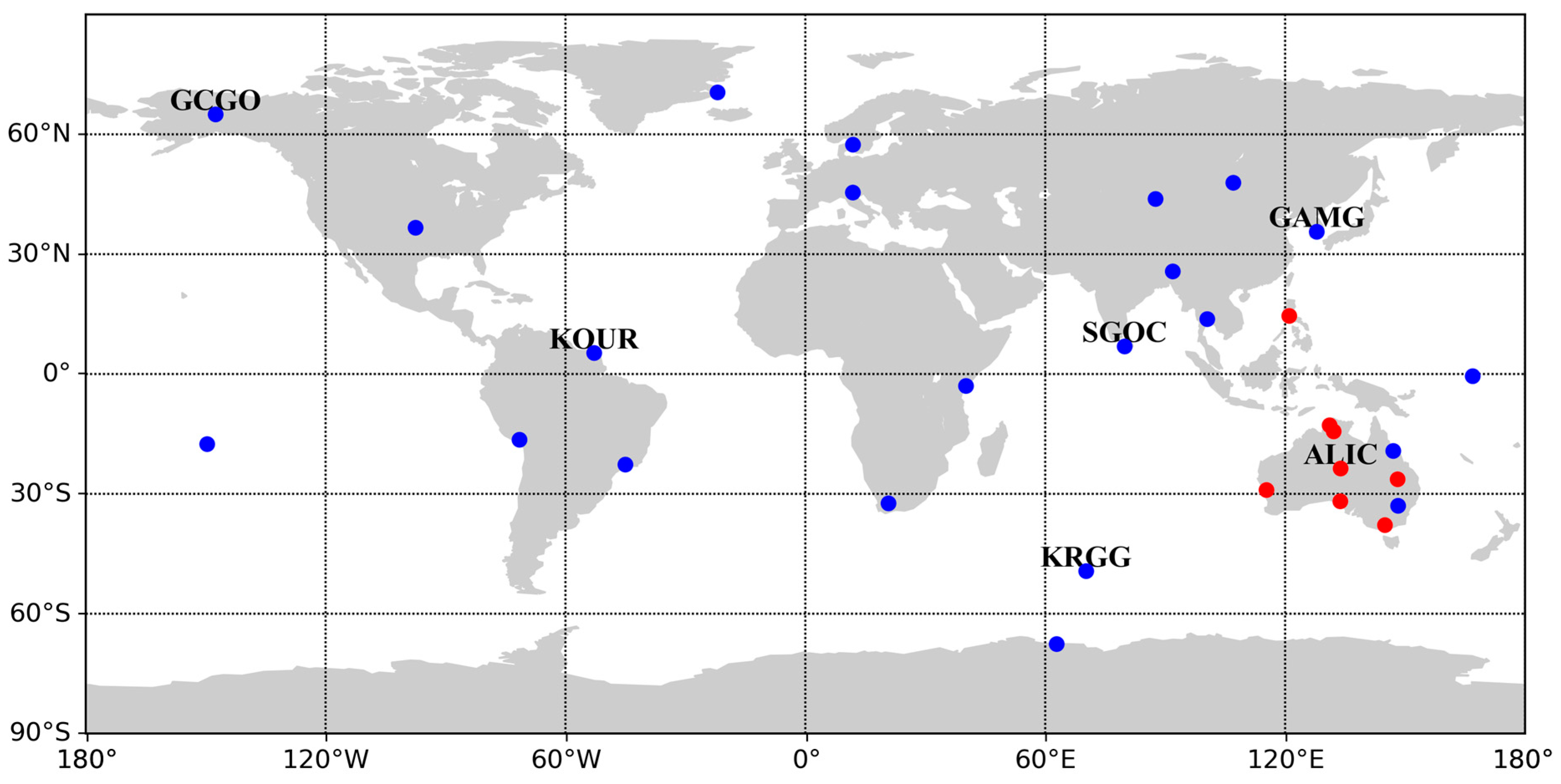
In order to analyze the characteristics of BDS SICB, the BDS observation data of more than 30 Multi-GNSS Experiment (MGEX) stations from the International GNSS Service (IGS) in different seasons were selected uniformly, as shown in

Table 1. Observation data period.

SICB	Data Period
Modeling Datasets	2022: Day of Year (DOY) 251–257, DOY 315–312, 2023: DOY 001–007, DOY 158–164,
Validation Dataset	2023: DOY 200–210

. The stations’ observation environment is ideal with minimal multipath effects. Only the stations located in East Asia and Australia can obtain complete and high quality IGSO satellite observation data. Therefore, when analyzing IGSO satellites, only the stations in East Asia and Australia are used. The distribution of the stations is shown in Figure 2. The red dots represent IGSO modeling stations, where all stations are used for MEO satellite modeling, and the outbound stations are labeled as subsequent algorithm verification stations.

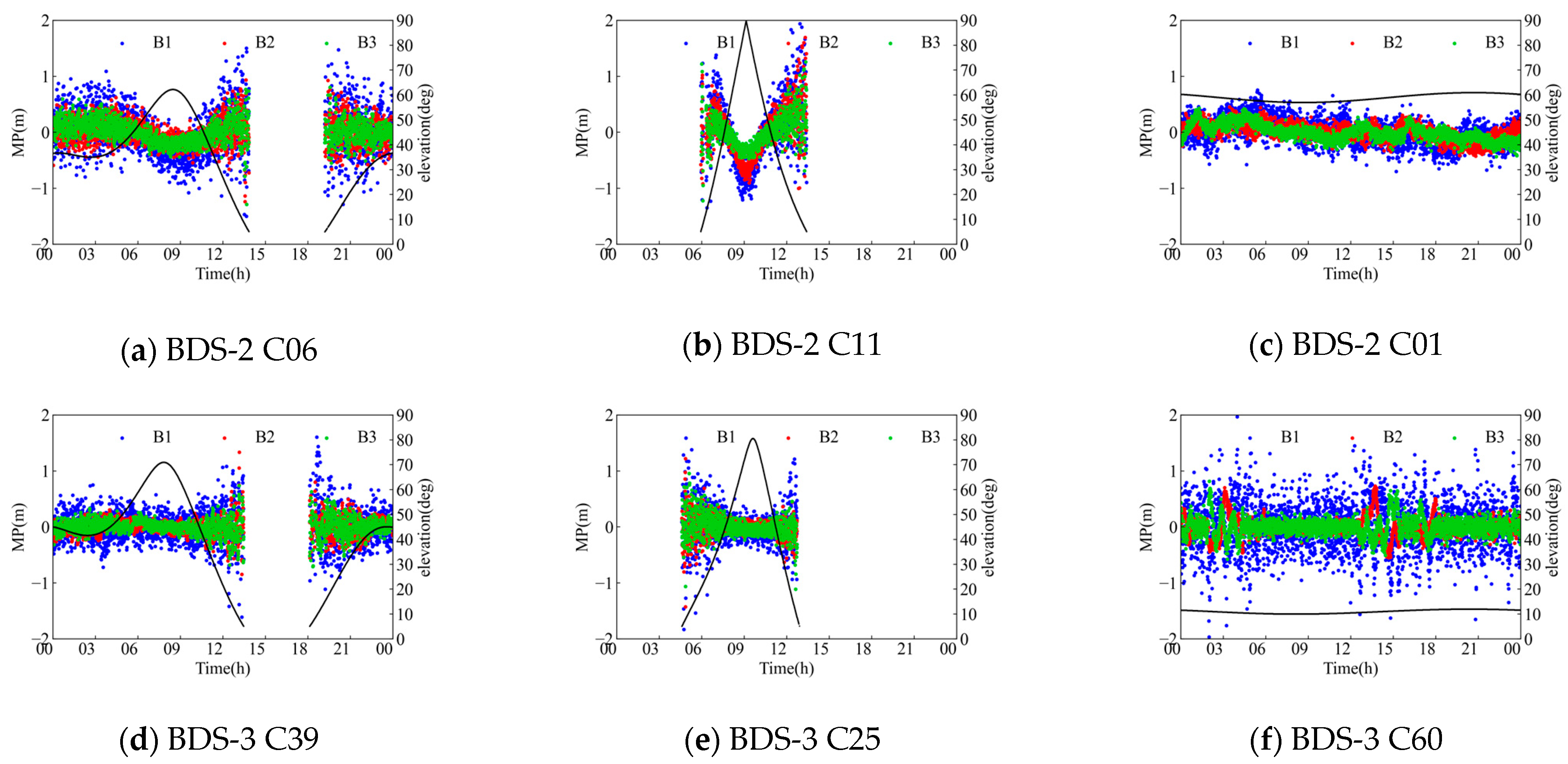
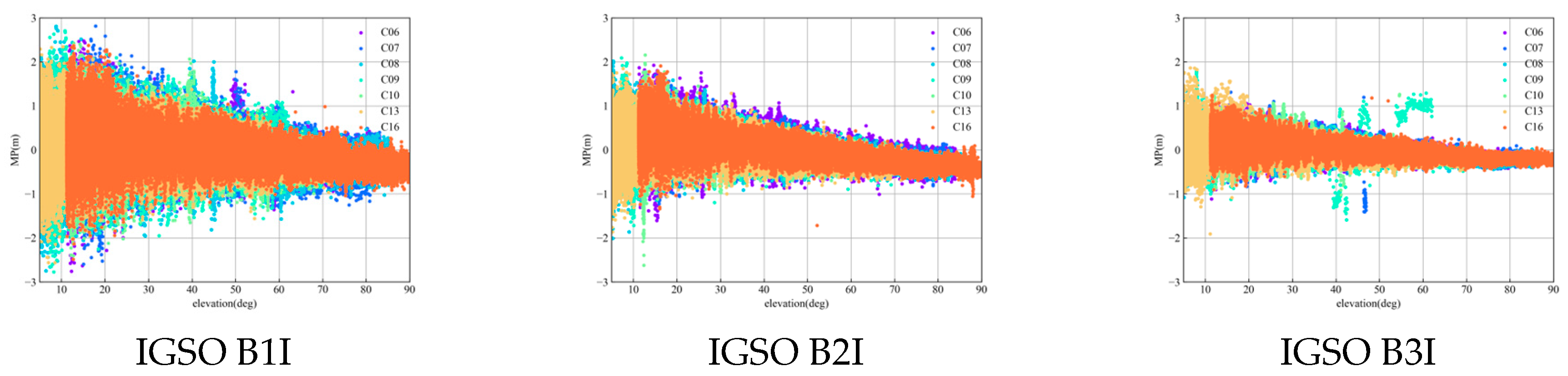
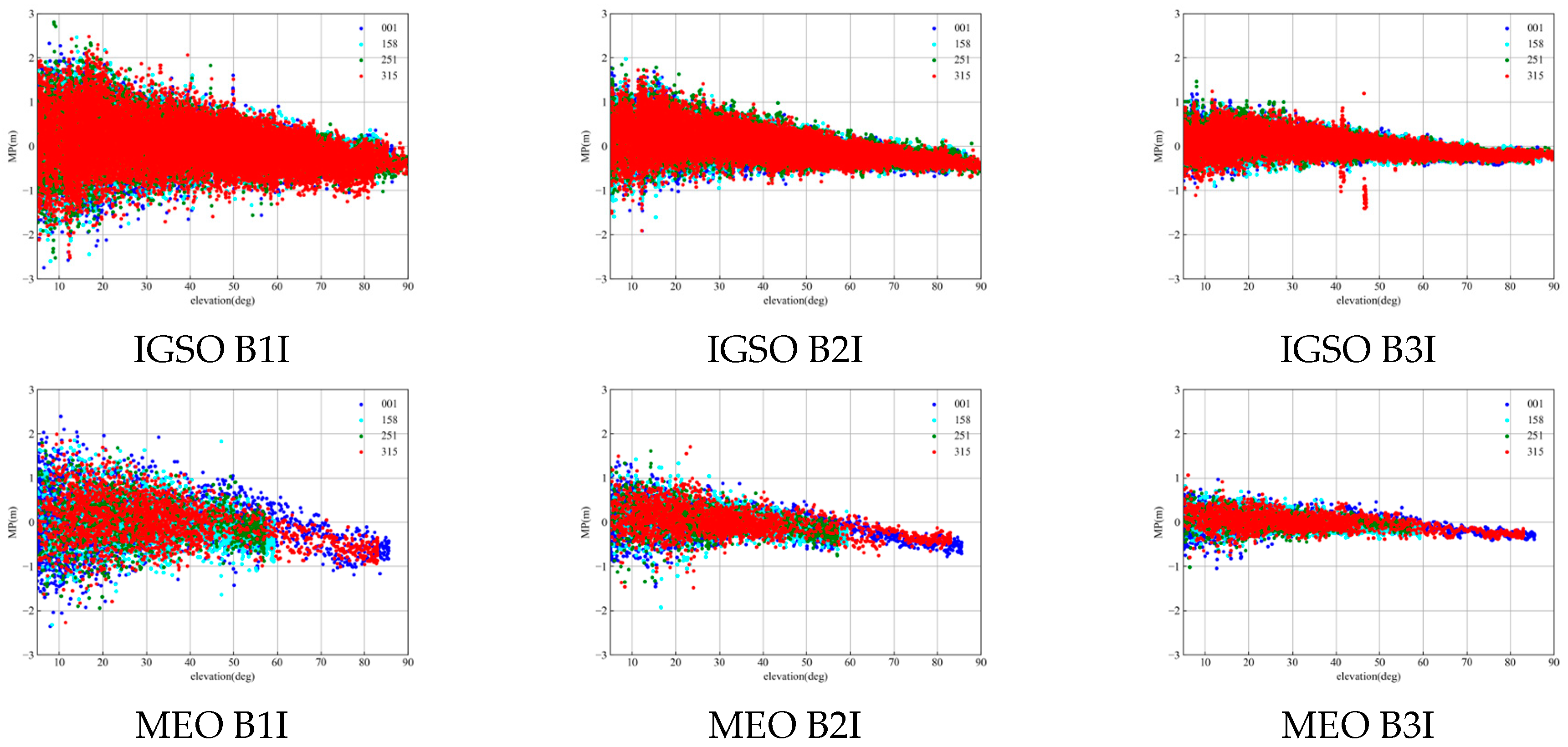
In order to explore the relationship between SICB and stations, seasons and satellites, we compare the MP and elevation angle of different satellites of same station, the MP and elevation angle of different stations, and the satellite elevation angle and MP of same station in different periods. Figure 3 shows the relationship between MP and the elevation of different satellites from the PPTG station. 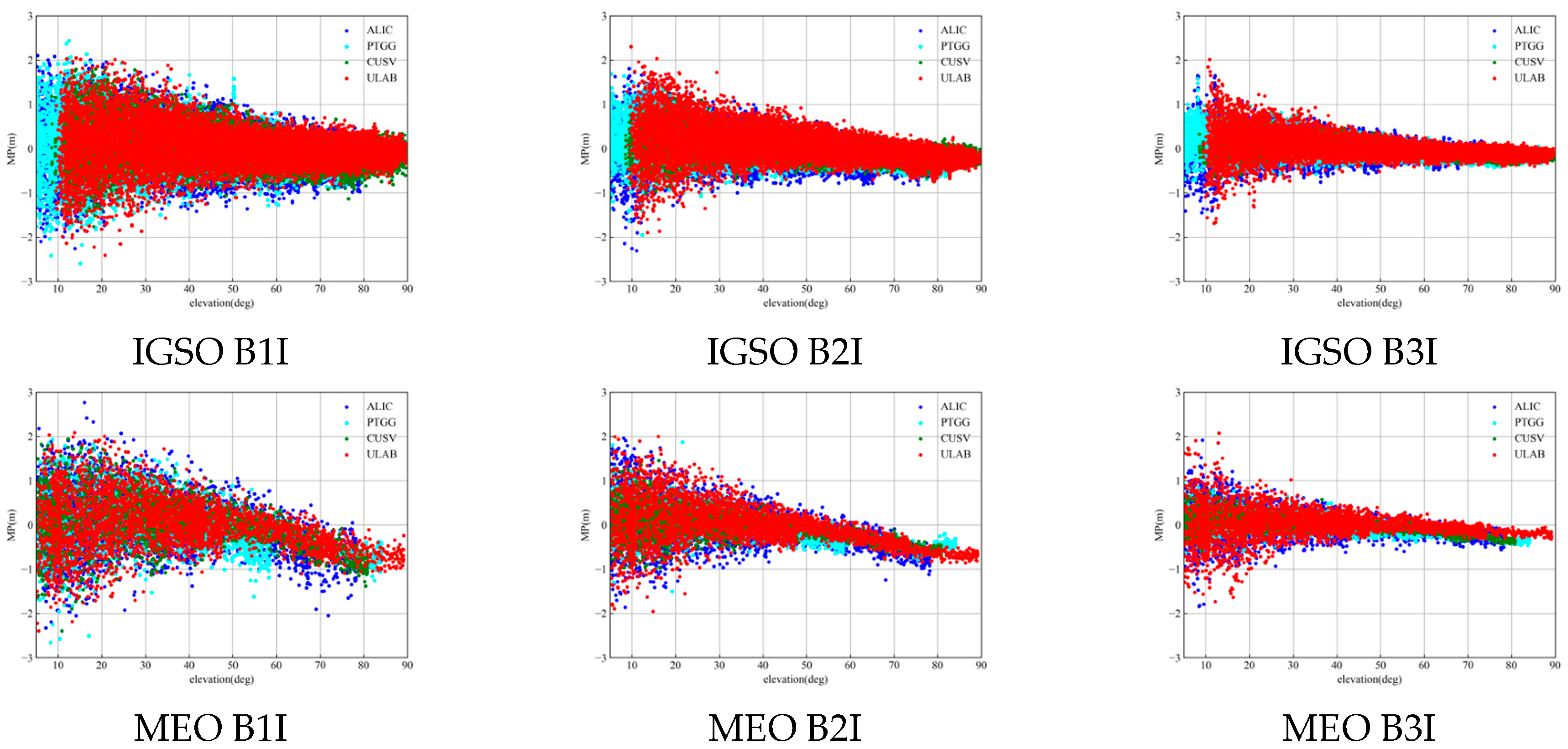Figure 4 shows the relationship between MP and the elevation angle of the ALIC, PTGG, CUSV, and ULAB stations at the same time. Figure 5 shows the relationship between MP and the elevation angle of PTGG stations at different dates (DOY001, 158, 251, and 315). SICB shows the same trend at different stations, with different satellites and times; however, it clearly differs at different frequencies. It is concluded that SICB is not related to the seasons, stations, and satellites, but is related to frequency.

To further investigate the correlation between the SICB and elevation angle, the Pearson correlation coefficient is calculated for all selected IGSO/MEO satellites at the chosen stations. The formula for the calculation is as follows:

$$Person=\frac{{\displaystyle \sum MP\cdot El-\frac{{\displaystyle \sum MP{\displaystyle \sum El}}}{N}}}{\sqrt{({\displaystyle \sum M{P}^2-\frac{{({\displaystyle \sum MP})}^2}{N}({\displaystyle \sum E{l}^2-\frac{{({\displaystyle \sum El})}^2}{N}})}}}$$

(12)

where $El$ and $N$ represent the elevation angle and the length of data, and $Person$ represents the correlation coefficient, with a range from −1 to 1. The larger the absolute value, the stronger the correlation. Coefficients between 0.2 and 0.4 indicate weak correlation, 0.4–0.6 indicate moderate correlation, 0.6–0.8 indicate strong correlation, and values greater than 0.8 indicate extremely strong correlation. The correlation coefficients are shown in

Table 2. Statistical table of elevation angle and MP correlation coefficient.

System	IGSO			MEO
	B1I	B2I/B2a	B3I	B1I	B2I/B2a	B3I
BDS-2	−0.2312	−0.3518	−0.2998	−0.3428	−0.3932	−0.2733
BDS-3	−0.0240	0.0143	0.0512	−0.0103	0.0422	−0.0181

.

The MP of BDS-2 IGSO/MEO is weakly negatively correlated with the elevation angle of the satellite. The MP of B2I is slightly higher than that of B1I and B3I. The MP between B1I, B2a, and B3I in BDS-3 is not correlated, indicating that the SICB of BDS-3 can be ignored. Therefore, this paper models and corrects the observation quantity of the BDS-2 satellite according to the IGSO/MEO satellite type.

This paper classifies satellite data based on IGSO/MEO, using an interval of 0.1 degrees, and takes the average value of MP that does not exceed 0.1 degrees. The Piecewise Third-Order Curve Fitting Method (TOCFM) with 30-degree nodes is used to fit the MP sequence, while also ensuring the global continuity of the nodes.

$$y=a_0+a_1\cdot El+a_2\cdot E{l}^2$$

(13)

where $y$ is the MP, El is the elevation angle, and $a_0$, $a_1$, $a_2$ are the three fitting coefficients. When the n epochs are observed, the MP value and elevation angle corresponding to each epoch can be obtained. The parameters ($a_0,a_1,a_2$) can be solved by using the least square method. The global fitting needs to satisfy the continuity of the boundary point. The minimum variance and the formula is as follows:

$$\left\{\begin{array}{l}{\displaystyle \sum _k^{m-1}{\displaystyle \sum _l^{n_k}{W}_{k,l}\cdot {(y_{k,l}-M{P}_{k,l})}^2}}=\min \\ y_k(E{l}_k)-y_{k+1}(E{l}_k)=0\end{array}\right.$$

(14)

where $k$ represents the segment point, $l$ represents the data epoch of the segment, and m and n represent the number of segments and the length of each segment, respectively.

The BDS MP time series shows significant noise at a low elevation. Considering the different accuracy of MP under different elevation angles, different weights are set for MP observations corresponding to different elevation angles in the fitting process. The weight design scheme is as follows:

$$W_{k,l}=a^2+\frac{a^2}{{\sin }^2(E{l}_{k,l})}$$

(15)

where a is usually 0.3, which is the pseudorange variance of the BDS observation, and $E{l}_{k,l}$ represents the elevation angle corresponding to point l in piecewise k.

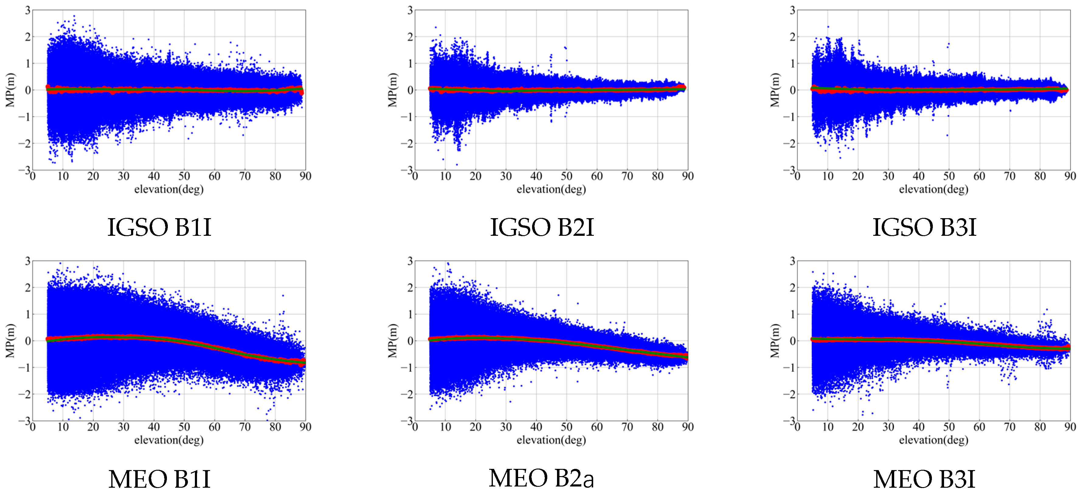
Figure 6 and

Table 3. Correction coefficients for SICB related to elevation angle.

Segmentation ($°$)	Parameter	IGSO			MEO
		B1I	B2I	B3I	B1I	B2I	B3I
5–30	$a_0$	0.0510	0.0883	0.0705	0.0434	0.0673	−0.0036
	$a_1$	0.0050	0.0074	0.0044	0.0024	0.0086	0.0137
	$a_2$	−6.14 × 10−5	−1.94 × 10−4	−1.54 × 10−4	−8.21 × 10−5	−2.69 × 10−4	−2.89 × 10−4
30–60	$a_0$	0.5297	0.5374	0.1706	−0.0233	0.0273	0.1153
	$a_1$	−0.0148	−0.0157	−0.0031	0.0059	0.0082	0.0201
	$a_2$	6.60 × 10−5	7.71 × 10−5	−1.79 × 10−5	−1.23 × 10−4	−2.10 × 10−4	−3.80 × 10−4
60–90	$a_0$	1.7007	0.7604	0.6366	0.9484	1.6042	2.7324
	$a_1$	−0.0513	−0.0219	−0.0188	−0.0252	−0.0423	−0.0702
	$a_2$	3.50 × 10−4	1.19 × 10−4	1.15 × 10−4	1.25 × 10−4	1.93 × 10−4	3.34 × 10−4

show that the fitting curve of BDS-3 is obviously close to 0, indicating that the BDS-3 SICB is small and negligible. The fitting curve of BDS-2 has different trends. Piecewise fitting can refine the SICB modeling at low elevation angles.

Figure 7 shows the comparison between the modeling results of a single station and multiple stations. The modeling trend of the single station and multi-station is the same, but there is a certain deviation in the value. The MP of B1I, B2I, and B3I have the same code bias trend and the value is slightly different.

Table 3 shows correction coefficients related to the MP time series and the elevation angle calculated by Equation (13) based on all observation data of the 30 stations around the world.

3.2. Analysis of the IGSO/MEO SICB Model Results

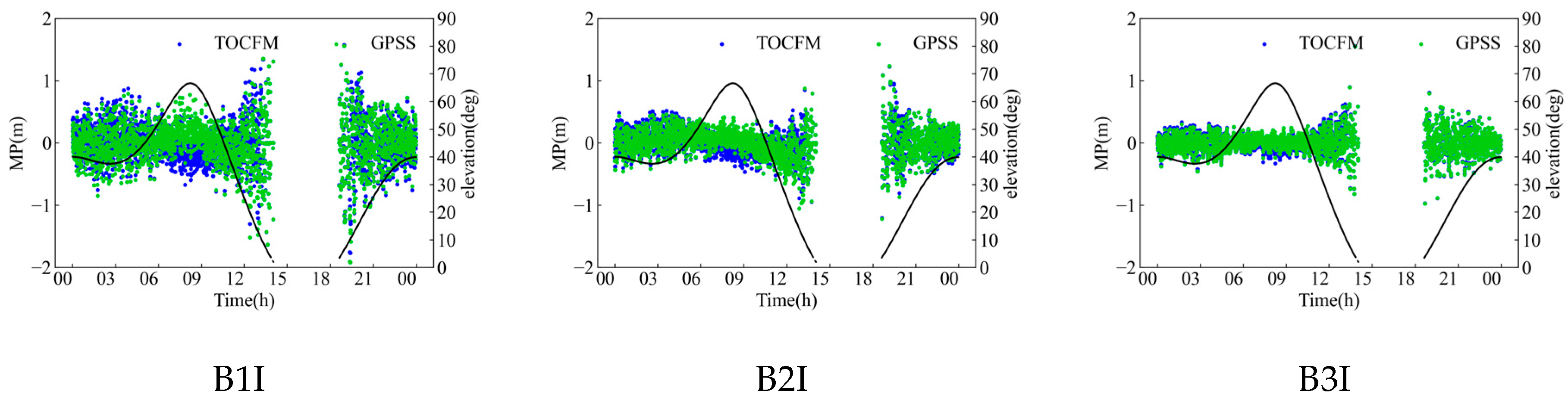
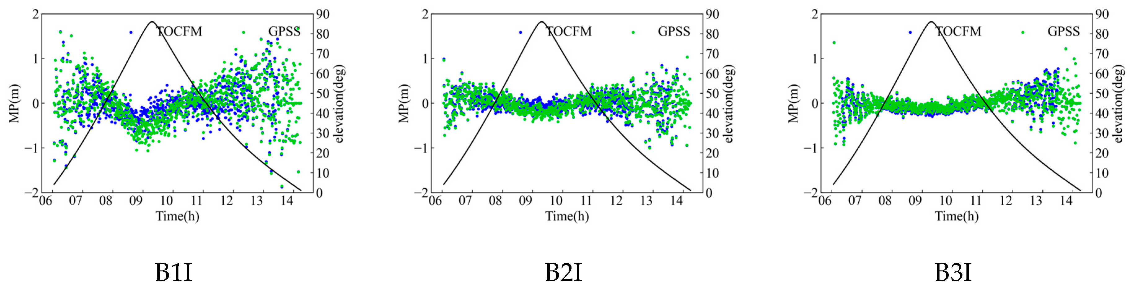
MP was corrected according to the correction coefficients of SICB calculated in Table 3. In order to verify the validity of the model, the correction coefficient of the reference [28] was compared (the model in the reference was named GPSS). Figure 8 and Figure 9 show the comparison of the correction effect between TOCFM and GPSS. The correction effect of TOCFM was better than that of GPSS at different elevation angles due to TOCFM adopting 0.1-degree interval piecewise fitting. Different correction effects indicate that different modeling data will produce different modeling coefficients.

In Figure 3, Figure 4, Figure 5, Figure 6, Figure 7, Figure 8 and Figure 9, it is evident that the MP of B1I exhibits the largest bias. B2I follows and B3I shows the smallest bias. After the correction, the SICB of IGSO/MEO satellites was effectively improved. Additionally, it can be observed that under the piecewise fitting method, the SICB at low elevation angles is mitigated to some extent.

3.3. SICB Correction Model of GEO Satellites

SICB modeling methods for GEO satellites, such as wavelet transform, regularization and machine learning methods. Variational Mode Decomposition (VMD) is a signal decomposition method that decomposes nonlinear non-stationary signals into a discrete number of modes. Compared to the widely used Empirical Mode Decomposition (EMD) method, it has the following advantages:

(1)

Through rigorous mathematical derivation, the theory is rigorous.

(2)

It overcomes the problem of modal aliasing in EMD.

(3)

It overcomes the breakpoint effect in EMD.

(4)

It has good noise and sampling robustness.

For detailed theory, please refer to [29].

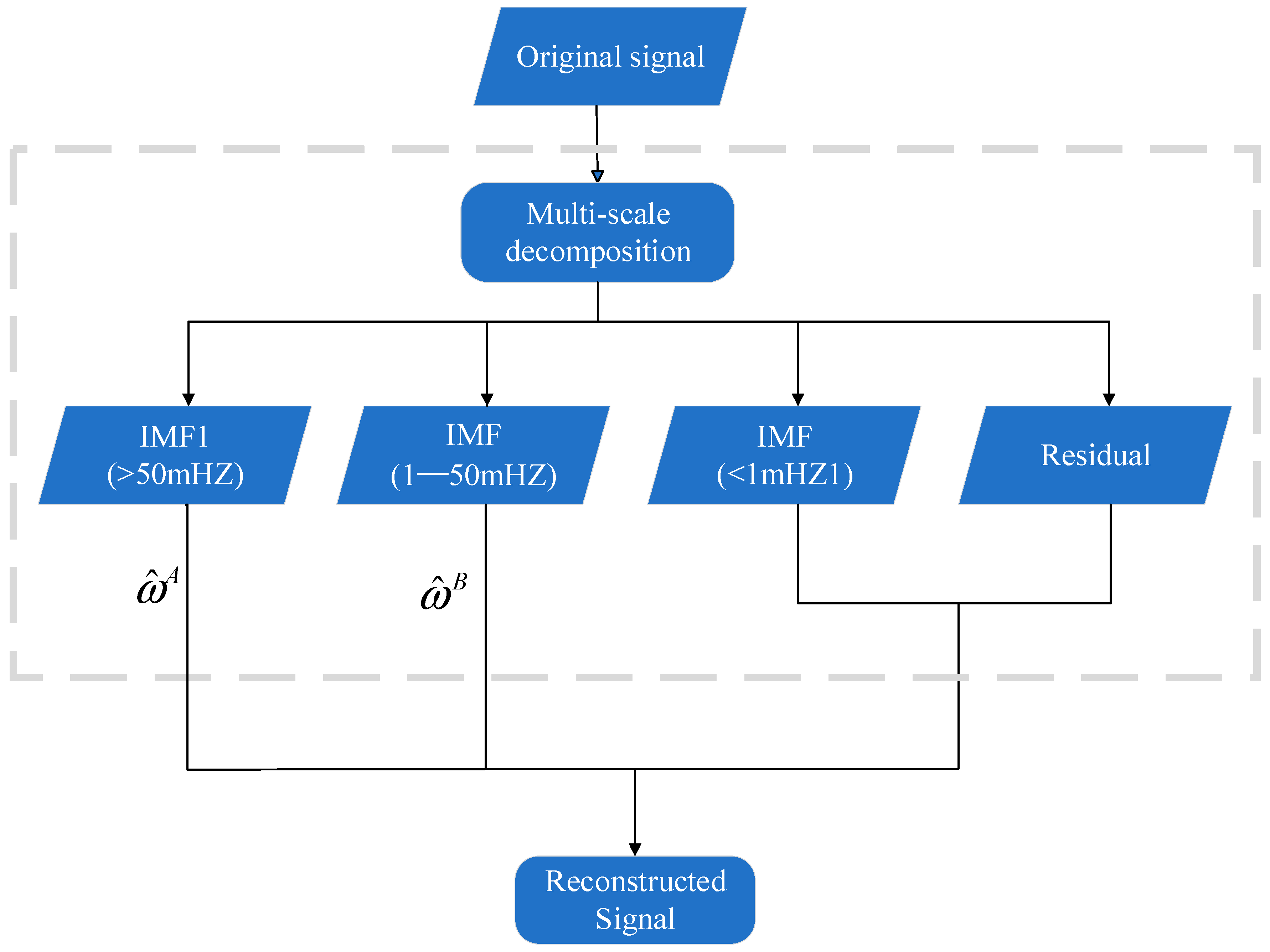
In this paper, we used the VMD-WT model to analyze and correct GEO SICB. It decomposes the original signal using VMD. Since each Intrinsic Mode Function (IMF) component has a different center frequency, different wavelet threshold functions are needed to improve the denoising effect. Therefore, different wavelet threshold functions are used for different IMF components.

The wavelet coefficients of the soft threshold function and adaptive threshold function are expressed as:

$${\widehat{\omega }}_{j,k}^A=\left\{\begin{array}{cc}\mathrm{sgn}({\omega }_{j,k}^A)(\left|{\omega }_{j,k}^A\right|-{\mu }_j^A),& \left|{\omega }_{j,k}^A\right|\ge {\mu }_j^A\\ 0,& \left|{\omega }_{j,k}^A\right|<{\mu }_j^A\end{array}\right.$$

(16)

$${\widehat{\omega }}_{j,k}^B=\left\{\begin{array}{cc}\mathrm{sgn}({\omega }_{j,k}^B)(\left|{\omega }_{j,k}^B\right|-\frac{{\mu }_j^B}{{({\left|{\omega }_{j,k}^B\right|}^2-{\left|{\mu }_j^B\right|}^2)}^J+1}),& \left|{\omega }_{j,k}^B\right|\ge {\mu }_j^B\\ 0,& \left|{\omega }_{j,k}^B\right|<{\mu }_j^B\end{array}\right.$$

(17)

where $\mathrm{sgn}(\cdot )$ is the sign function, ${\widehat{\omega }}_{j,k}^A$, ${\widehat{\omega }}_{j,k}^B$ are the k-th wavelet coefficients of the j-th layer after the DWT, and $J$ is the total number of wavelet reconstruction layers. In addition, the threshold ${\mu }_j^A$ and threshold ${\mu }_j^B$ are calculated from:

$$\left\{\begin{array}{l}{\mu }_j^A={\sigma }_j\sqrt{2\ln (N_j)}\\ {\mu }_j^B={\sigma }_j\sqrt{2\ln (N_j)}/\ln (j+1)\end{array}\right.$$

(18)

where the current number of reconstruction layers is j, the noise standard deviation is ${\sigma }_j=median(\left|{\omega }_{j,k}\right|)/0.6745$, and $N_j$ is expressed as the length of the current reconstruction layer.

The principle of VMD-WT is to maximize the noise reduction performance while maintaining the local characteristics of the original signal. Soft thresholding can reduce signal loss in high-frequency signals. The adaptive threshold function is used to remove noise components in the MP time series. It can also avoid the constant bias of soft thresholding and the discontinuity of hard thresholding. The recommended frequency is 50 mHZ under good observation conditions. This particular setup is the best choice for obtaining precise results in this situation. The data processing flow is shown in Figure 10.

3.4. Analysis of the GEO Correction Results

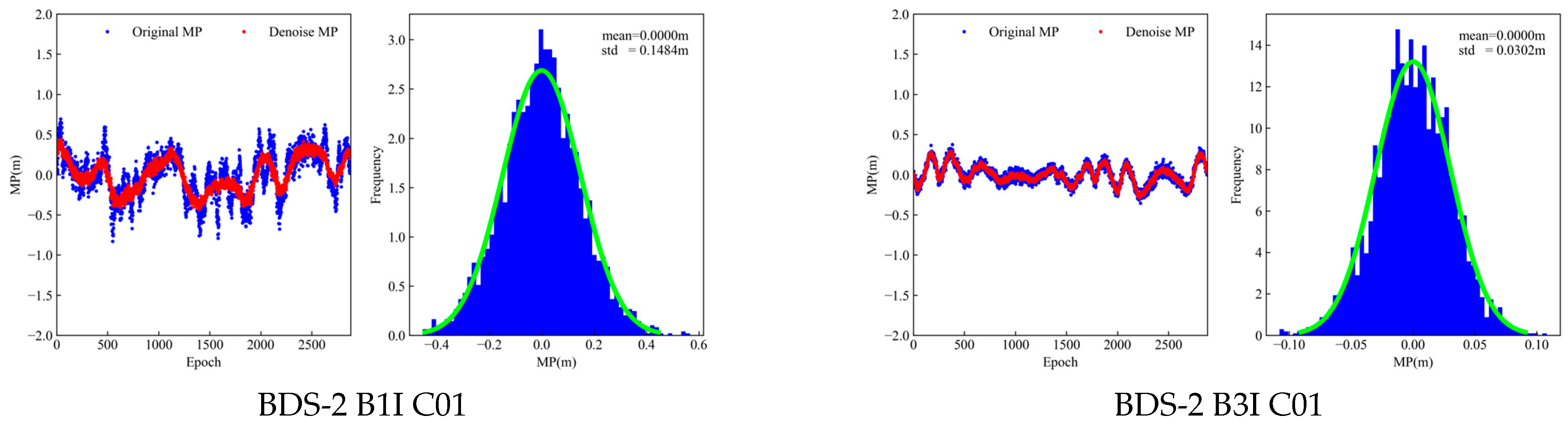
Figure 11 shows the MP result of C01, C04, C59, and C60 processed by VMD-WT with ALIC at DOY 200. The left side shows the original MP and the denoised MP. The right side shows the residual histogram of MP. The corrected residuals approximate normal distribution and are very close to white noise.

Table 4. Reduction percentage of the MP (%).

Frequency	C01	C02	C03	C04	C05	C59	C60	C61	Average
B1I	60.6	50.6	28.9	65.9	47.9	66.0	50.7	56.2	53.35
B2I	69.0	57.8	51.8	71.9	67.0				63.50
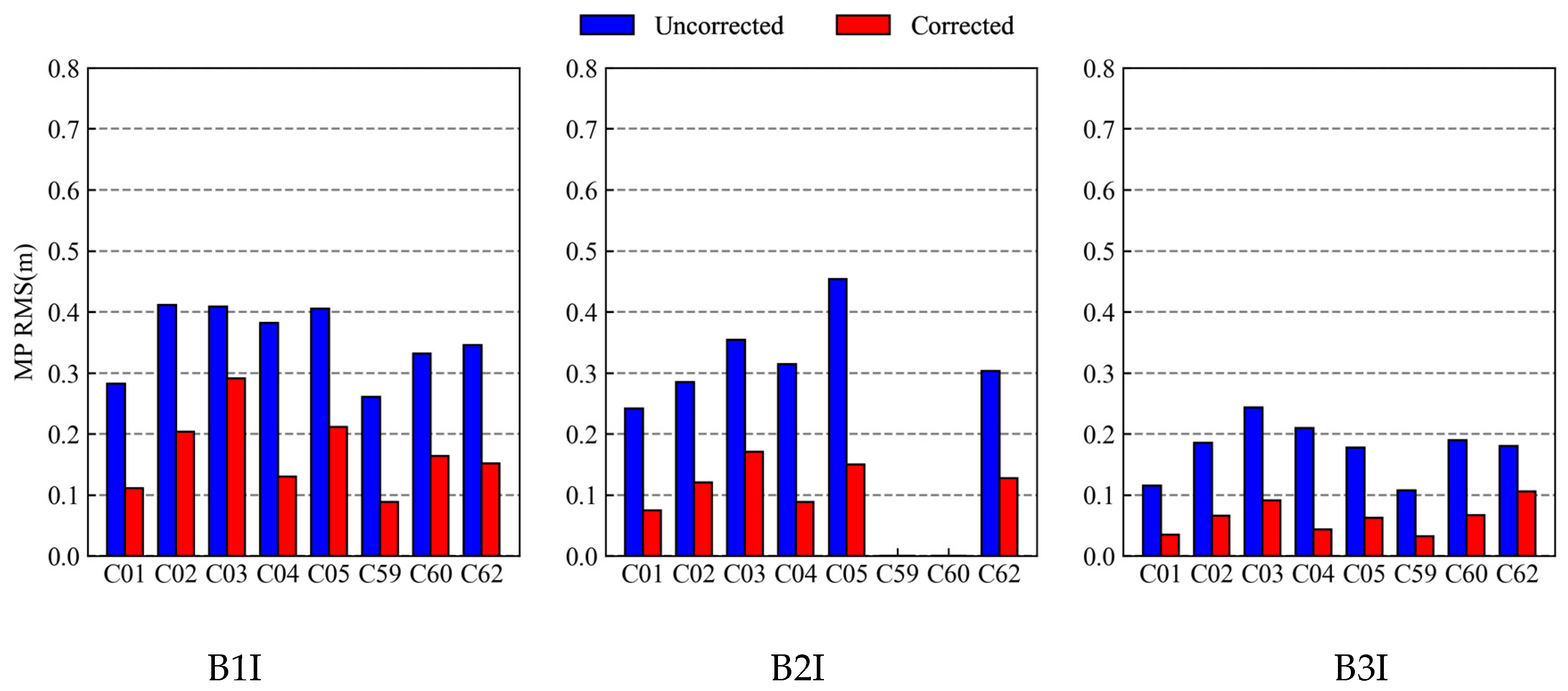
B3I	69.9	64.5	62.5	79.5	65.0	70.5	64.7	41.1	64.71

provides the detailed improvement ratio before and after the correction. The Root Mean Square Error (RMSE) of the modified MP time series decreased significantly and the RMSE of B1I, B2I, and B3I decreased by 53.35%, 63.50%, and 64.71%, respectively. Figure 12 shows the uncorrected and corrected MP RMSE of six GEO satellites at all stations (C05 was not corrected due to missing data at some stations).

Figure 11 and Figure 12 show that VMD-WT can perform better noise reduction on GEO satellites and the residual error after the correction is basically in a normal distribution, with an average increase of about 60%. At the same time, it was found that the multipath of the BDS-3 satellite was different from that of the BDS-2 satellite.

3.5. Correction of the SICB to Improve the CSC of the BDS

To verify the effectiveness of the algorithm, different time periods from the SICB modeling data were selected. The experiment was conducted based on the experimental data from 6 stations, ALIC, KRGG, KOUR, GCGO, GAMG, and SGOC, from 19 July 2023 to 29 July 2023. Four strategies were used for BDS SPP: Scheme 1: Ionosphere-free single point positioning (IF SPP), Scheme 2: ionosphere-free CSC single point positioning (IF CSC SPP), Scheme 3: CSC single point positioning with the IGSO/MEO SICB Correction based on the TOCFA Method (IGSO/MEO SICB CSC), and Scheme 4: CSC single point positioning with the IGSO/MEO/GEO SICB correction based on VMD-WT and TOCFA (IGSO/MEO/GEO SICB CSC). The processing strategy is shown in

Table 5. Processing strategies of the SPP for the BDS.

Parameters	Models
Observations	Raw observations
Signal	BDS B1I/B3I
Sampling rate	30 s
Cycle slip detection	GF and MW
Smooth window	20 (min)
Smoothing factor	20
Elevation cutoff	${10}^{°}$
Relativistic effect	Corrected
Ionospheric delay	Ionosphere-free combination
Tropospheric delay	Saastamoinen
Estimator	Weighted least squares

.

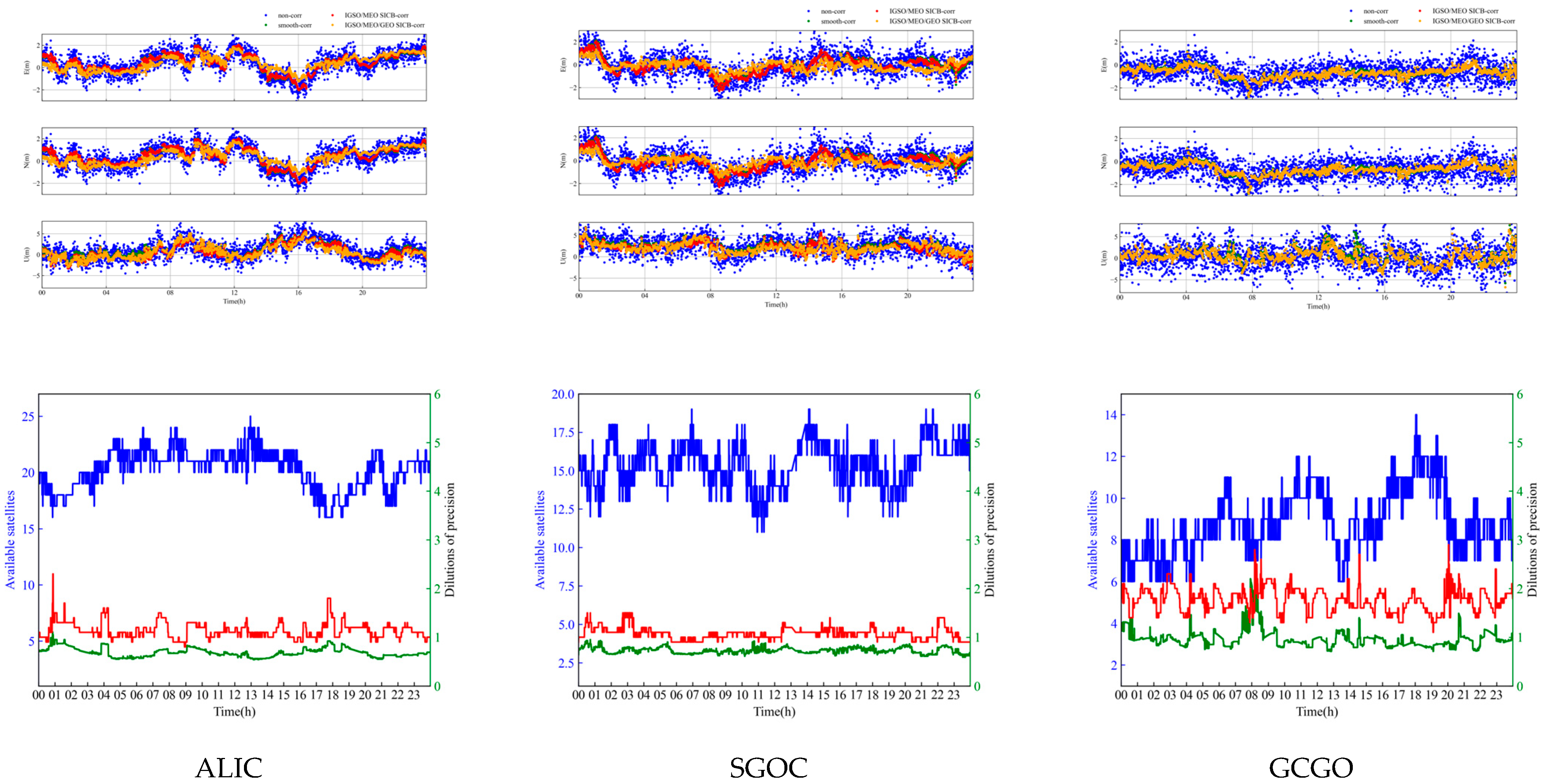
The E, N, and U direction residuals, the number of available satellites, Horizontal Dilution of Precision (HDOP), and Vertical Dilution of Precision (VDOP) of the three stations are shown in Figure 13. The weekly solution document coordinates were used as reference values. The satellite elevation angle and pseudorange residuals are shown in Figure 14.

Table 6. Positioning errors for the BDS SPP with four different strategies.

Station		RMSE				Improvement Rate#-Previous (%)
		E	N	U	3D	E	N	U	3D
ALIC	Scheme 1	0.939	0.770	2.210	2.521
	Scheme 2	0.784	0.579	1.751	2.004	16.414	24.774	20.749	20.498
	Scheme 3	0.807	0.570	1.569	1.854	−2.893	1.623	10.406	7.496
	Scheme 4	0.688	0.531	1.461	1.700	14.762	6.765	6.880	8.310
KRGG	Scheme 1	0.579	0.877	1.508	1.838
	Scheme 2	0.502	0.786	1.346	1.637	13.381	10.333	10.776	10.930
	Scheme 3	0.491	0.772	1.207	1.515	2.228	1.812	10.264	7.478
	Scheme 4	0.486	0.791	1.199	1.507	0.866	−2.511	0.681	0.522
KOUR	Scheme 1	1.210	0.896	2.871	3.242
	Scheme 2	1.043	0.733	2.547	2.849	13.741	18.239	11.275	12.129
	Scheme 3	1.032	0.723	2.501	2.800	1.132	1.330	1.836	1.707
	Scheme 4	1.032	0.723	2.501	2.800	0.000	0.000	0.000	0.000
GCGO	Scheme 1	1.019	1.312	3.083	3.502
	Scheme 2	0.764	0.714	2.133	2.375	25.041	45.591	30.826	32.179
	Scheme 3	0.777	0.691	1.927	2.189	−1.721	3.235	9.657	7.824
	Scheme 4	0.777	0.691	1.927	2.189	0.000	0.000	0.000	0.000
GAMG	Scheme 1	0.735	0.706	2.324	2.538
	Scheme 2	0.609	0.558	2.087	2.245	17.044	20.992	10.189	11.538
	Scheme 3	0.635	0.563	1.870	2.054	−4.207	−1.010	10.411	8.516
	Scheme 4	0.593	0.500	1.820	1.978	6.579	11.186	2.682	3.664
SGOC	Scheme 1	0.964	0.789	3.242	3.473
	Scheme 2	0.714	0.495	2.819	2.949	25.980	37.247	13.064	15.084
	Scheme 3	0.679	0.468	2.515	2.647	4.857	5.553	10.762	10.255
	Scheme 4	0.620	0.459	2.468	2.585	8.731	1.983	1.885	2.324

shows the RMSE in the E, N, and U directions of four different schemes for 11 consecutive days and the improvement ratio of the current scheme compared to the previous scheme.

Figure 13 and Figure 14 and Table 6 show that the positioning accuracy gradually improves with the addition of the IGSO/MEO/GEO SICB correction. The improvement effect was evident in the U direction. At the same time, SICB negatively impacts the accuracy of the E direction because SICB greatly impacts on the U direction more than the E direction, which is consistent with the characteristics of SICB in previous studies.

In the case of only adding the IGSO/MEO SICB correction, the positioning accuracy of the ALIC and SGOC stations has the best improvement. Figure 14 shows that the elevation angles of the satellites of the two stations are generally higher, so the pseudorange was greatly affected by SICB. The effect of the SICB correction is remarkable. Due to the difference in elevation of IGSO/MEO satellites at the KOUR and GCGO stations, the improvement effect was also different. The 3D RMSE of the two stations was reduced to 7.824% and 8.516%, respectively.

After adding the GEO SICB correction, the positioning accuracy of the E and U directions was improved. The highest improvement was the ALIC station and the E, N, and U directions were improved by 14.762%, 6.765%, and 6.880%, respectively, due to the fact that the ALIC station observes more GEO satellites. The improvement effect of the KRGG station was the worst, with an increase of 14.762%, 6.765%, and 6.880% in the E, N, and U directions, respectively. This is due to the lack of available GEO satellites at the KRGG station. Since KOUR and GCGO stations are not located in Asia or Australia, GEO satellites cannot be observed or are below the cut-off satellite elevation angle, so Scheme 4 has no change compared with Scheme 3. The SICB correction of GEO satellites was significant when multiple GEO satellites are observed.

In the case of the IGSO/MEO/GEO satellite SICB correction, the average improvement rate between Scheme 4 and Scheme 2 in the E, N, and U directions was 7.03%, 6.49%, and 10.48%, respectively. The IGSO/MEO/GEO CSC algorithm can improve the positioning accuracy by 9%~10% compared to the traditional IF SPP CSC algorithm.

In summary, the improvement effect of SICB is related to the elevation angle of the satellite and indirectly to the station’s position. Under normal circumstances, the accuracy after the IGSO/MEO SICB correction can be increased by 7% to 10% and the accuracy after the GEO SICB correction can be increased by 2% to 8%.

In particular, we also analyze the effect of SICB on the BDS B1/B3 ionosphere-free combination PPP model and find that the impact was not significant. Therefore, the calculation process and results are not given in this paper.

4. Conclusions

This paper reviews the basic principles of CSC and performs error analysis. Through the correlation analysis between MP and elevation angle, the MP of BDS-2 IGSO/MEO has a weak negative correlation with the elevation angle of the satellite, which indirectly indicates that there was a systematic bias between the pseudorange observation and the carrier observation of the BDS 2 IGSO/MEO satellite; that is, SICB. The proposed TOCFM is slightly better than the methods in reference [28]. The IGSO/MEO piecewise weighted least squares TOCFM SICB correction model was established by acquiring the MP time series from 30 stations worldwide. For GEO satellite SICB, a variational mode decomposition combined with the wavelet transform (VMD-WT) method is proposed. The MP time series RMSE of GEO B1I, B2I, and B3I are reduced by 53.35%, 63.50%, and 64.71%, respectively. Based on the above, we propose the CSC algorithm, considering that IGSO/MEO/GEO SICB is proposed in this paper.

In order to verify the effectiveness of the SICB correction, the effects on IF SPP CSC before and after the SICB correction were analyzed and compared. The results show that the SICB correction model effectively weakens the SICB and improves the positioning accuracy of CSC SPP. The accuracy after the IGSO/MEO SICB correction can be increased by 7%~10%, and the accuracy after the GEO SICB correction can be increased by 2%~8%. Therefore, The SICB plays an important role in improving the positioning accuracy. The SICB correction algorithm applies to all smooth pseudorange algorithms and only the dual-frequency IF-CSC algorithm is computed in this paper.

However, there are some shortcomings. It should be noted that the accuracy improvement may be limited in challenging environments due to the influence of cycle slips. Additionally, the model of IGSO/MEO SICB has yet to be modeled for each satellite, leaving room for further improvement in the positioning accuracy. Based on previous research, the characteristics of the different GEO satellite SICB is different and the effect of the different denoising strategy is not the same. Therefore, the Doppler smoothing pseudorange and IGSO/MEO SICB accurate modeling will be the focus of further research. Also, since CCL/CSC is widely used in GNSS ionospheric modeling, we will focus on evaluating the application performance of these two methods in the future.