Abstract
Ecosystem water use efficiency (WUE) and ecosystem photosynthetic efficiency (EPE) are key indicators in studies of the carbon–water cycle in terrestrial ecosystems. Analyses of WUE and EPE can enhance our understanding of the relationship between ecosystem light use efficiency and WUE. Although several studies of individual indexes (i.e., either WUE or EPE) have been conducted, analyses of variation in both WUE and EPE, as well as their relationships, have rarely been conducted. Here, we analyzed spatial and temporal variation in WUE and EPE in Central Asia. Specifically, time trend analysis was conducted to characterize temporal and spatial changes in WUE and EPE in Central Asia from 2001 to 2020 at different altitudes and latitudes. Pearson correlation analysis was used to characterize the effects of precipitation and temperature on WUE and EPE. WUE decreased and EPE increased in Central Asia over the 20-year study period; this might have been due to interannual variations in precipitation and temperature. WUE was highest in August, and EPE was highest in June and July. Substantial spatial heterogeneity in WUE and EPE was observed; WUE was highly variable in Central Asia as well as in western and southern Central Asia. Major changes in EPE were observed in northern, eastern, and southern Central Asia. We also found that both WUE and EPE decreased with the increase in altitude. WUE was positively correlated with temperature and negatively correlated with precipitation, whereas EPE was positively correlated with both temperature and precipitation. The increase in photosynthetic efficiency might be one of the main factors contributing to increases in ecosystem productivity in arid environments. The temporal and spatial variation in WUE and EPE observed in our study will aid ecosystem research, providing a reliable theoretical basis for ecosystem research in areas with scarce large-scale data, integrated water resources management, and ecosystem restoration efforts. Our findings also enhance our understanding of the terrestrial carbon–water cycle and have implications for predicting ecosystem responses to climate change. The results of this study provide insights that will aid studies of the terrestrial carbon–water cycle under the background of climate change. It is of great significance to further study the carbon water cycle in the future.
1. Introduction
Vegetation is a major component of terrestrial ecosystems that links the soil, hydrosphere, and atmosphere; it plays a key role in modulating the carbon and water balance of terrestrial ecosystems [1]. Environmental factors such as light, temperature, and water have major effects on the growth and spatial distribution of vegetation. Increases in atmospheric carbon dioxide (CO2) concentrations, the intensity and frequency of droughts, and the occurrence of extreme climatic events have resulted in changes in the structure and function of ecosystems, such as the death of vegetation, reductions in forest area, desertification, and even the irreversible degradation of ecosystems [2,3,4,5]. Water and light are important raw materials for the photosynthesis of plant leaves; they also have major effects on the stability of ecosystems as well as ecosystem changes.
The definitions of WUE are manifold. At the ecosystem level, WUE is defined as the ratio of the gross primary product of vegetation (GPP) to evapotranspiration (ET) [6,7,8,9]. WUE is an important measure of ecosystem function; it is also an important indicator of the degree of coupling between the carbon–water cycle and ecosystem water use strategies. It can thus be used to evaluate the responses of ecosystems to environmental change. Spatial and temporal changes in ecosystem WUE are mainly affected by topographic features, climate, plant functional types, and the physiological regulation of the stomata [10,11,12]. Previous studies have indicated that the main factors driving variation in WUE include latitude, altitude, temperature, precipitation, leaf area index (LAI), vapor pressure deficit (VPD), soil moisture, enhanced vegetation index, CO2 concentration, and other factors [4,13,14,15,16]. Therefore, in this study, we analyzed the influence of the relationship between precipitation and temperature on WUE and EPE and analyzed the effects of altitude and latitude under different gradients on the WUE and EPE of different vegetation types. Li et al. obtained solar-induced chlorophyll fluorescence (SIF) data with a spatial resolution of 0.05° using a data-driven approach [17]. SIF is generated via the photosynthesis of terrestrial vegetation [18]; research on SIF could provide insights into the function of vegetation and the terrestrial carbon cycle [19]. Previous studies have revealed a linear relationship between SIF and GPP at the ecosystem scale [20,21]. Many studies have examined the global carbon cycle using estimates of SIF [22]. Wei et al. proposed the metric ecosystem photosynthetic efficiency (EPE) to characterize the relationship between the carbon sequestration rate and the greening of the earth; it is calculated using SIF and LAI [23]. Most previous studies on WUE and EPE have focused on analyzing changes in individual indices and the factors driving these changes. However, few studies have examined changes in both of these indicators and the factors driving these changes. The analysis of temporal and spatial changes in WUE and EPE and the factors driving these changes could enhance our understanding of the responses of ecosystems to climate change and offer insights into the relationship between water and carbon.
Arid ecosystems are sensitive to climate change, and the biological diversity of arid ecosystems is unique [24]. Changes in arid ecosystems can be mediated by both natural and anthropogenic factors. There is still much to learn regarding the spatial and temporal relationships between WUE and EPE, as well as the factors driving variation in the relationship between WUE and EPE, in arid areas. Papanatsiou et al. showed that stomatal conductance might enhance WUE [25]. Jasechko et al. made water resource predictions indicating that improvements in the simulation of biological flux should be prioritized in the development of climate models [26]. Li et al. showed that LAI was the major factor driving changes in WUE [17]; other important factors affecting changes in WUE included the atmospheric CO2 concentration and VPD [27]. Wei et al. found that soil moisture was a key factor affecting changes in EPE [23]. Poulter et al. showed that the growth in semi-arid vegetation in the Southern Hemisphere is the cause of global carbon sink anomalies [28].
Remote-sensing technology has been used to characterize changes in the ecosystem carbon–water cycle, as well as the factors driving these changes, at global and regional scales, and several valuable insights have been provided by the corresponding studies [6,29]. Central Asia is one of the world’s largest arid regions at the mid-latitudes [30]. The ecosystem of Central Asia is fragile, and this region currently faces several major ecological problems [31,32,33]. The carbon cycle and energy in the relationship between the atmosphere and land in this region are affected by changes in the natural environment, so these cycles exhibit unique spatial and temporal characteristics [34]. Research shows that a decrease in precipitation and a rise in temperature can lead to severe droughts in Central Asia, and these changes may affect vegetation growth and the ecosystem in Central Asia [35]. In this study, using MODIS satellite data and the GOSIF dataset developed and processed by Li et al. [17], the values of WUE and EPE in Central Asia during 2001–2020 were calculated, and the spatial and temporal variation characteristics were analyzed. We also analyzed correlations of climate factors with WUE and EPE in this region over the study period. The main aims of our study were to (1) clarify spatial and temporal patterns in WUE and EPE and the relationship between changes in WUE and EPE; (2) characterize changes in the WUE and EPE of different vegetation types with respect to altitude and latitude; and (3) determine the effects of precipitation and temperature on WUE and EPE. Analyses of changes in WUE and EPE at different spatial and temporal scales in arid ecosystems could provide insights that would aid the monitoring of the carbon–water cycle and vegetation in terrestrial ecosystems. Such studies also provide important information for carbon and water balance predictions that could aid in the sustainable management of water resources in areas with fragile ecosystems. Lastly, such studies can enhance the ac-curacy of predictions of the direction of future climate change, and this affordance has key implications for the sustainable development of human society.
2. Study Area
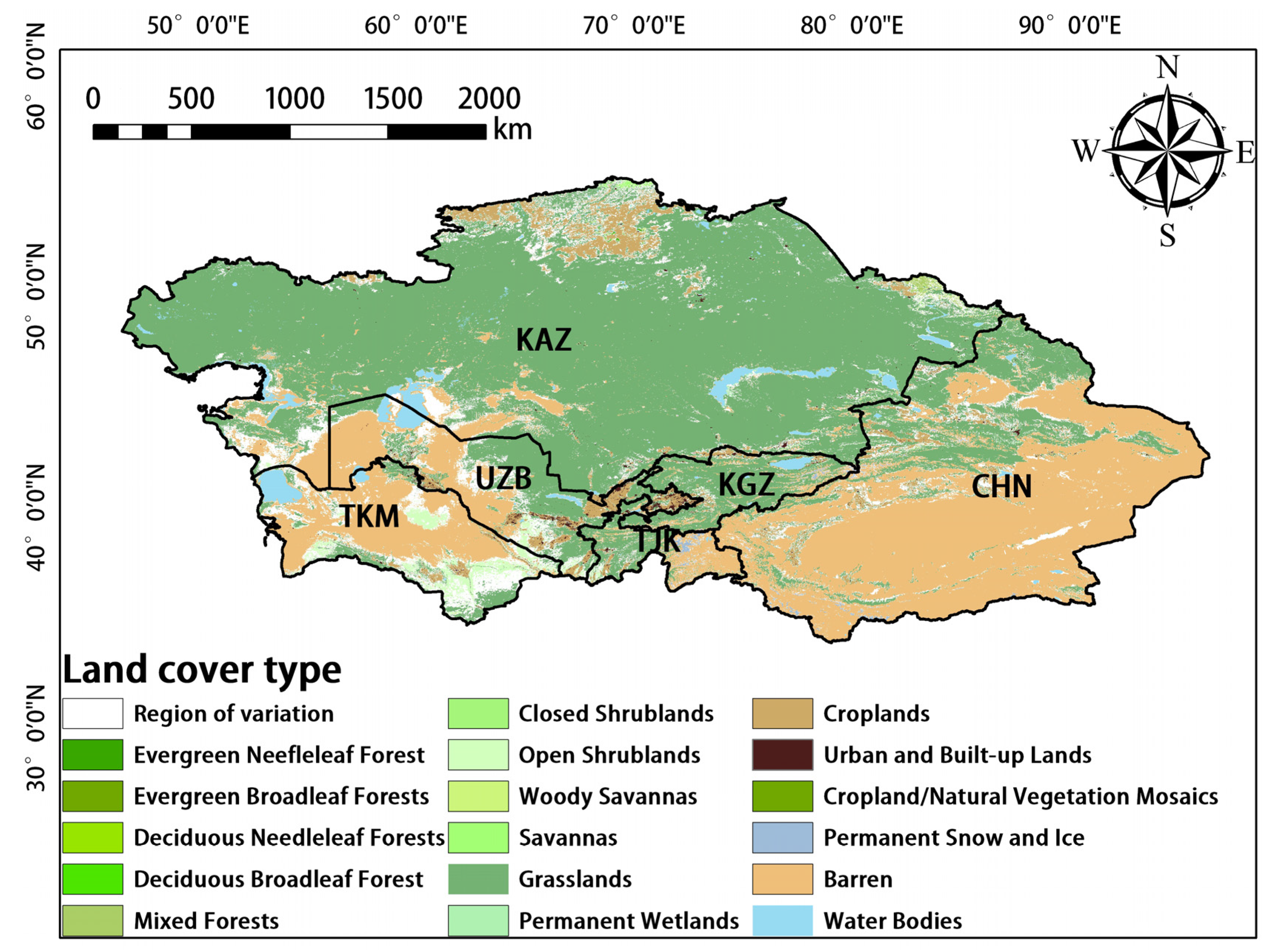
Central Asia denotes the central region of Asia; however, there is no consensus on the geographical units that comprise this region [36]. In our study, we follow the definition of Central Asia given in a study conducted by Deng et al. [37], in which it was proposed that Central Asia comprises Kazakhstan, Turkmenistan, Uzbekistan, Kyrgyzstan, Tajikistan, and China’s Xinjiang Uygur Autonomous Region (Figure 1) [38]. Central Asia has a temperate continental climate. The altitude of this region is higher in the east and lower in the west, and the decrease in altitude from east to west is gradual. The climate changes from semi-arid to arid from north to south. Evapotranspiration is strong, and temperatures are low in the winter and high in the summer; there is a large temperature difference between day and night, and sunshine is abundant [38]. These conditions are suitable for the growth of crops. The northern portion of Central Asia mainly comprises rain-fed agricultural land, and irrigated areas are abundant in southern Central Asia [39]. Because the altitude in this region is high in the southeast and low in the northwest, the rivers flow from southeast to northwest. The growing period spans from April to October and can be divided into three seasons: spring (April and May), summer (June and August), and autumn (September and October) [40].
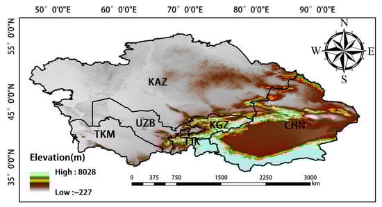
Figure 1.
Map of the study area.
3. Methods
3.1. Data Sources
3.1.1. Moderate-Resolution Imaging Spectroradiometer (MODIS) Data
MODIS data [41] were downloaded from the National Aeronautics and Space Administration (NASA) website (https://modis.gsfc.nasa.gov/ (accessed on 22 August 2022)). The MODIS sensors deployed on the NASA Terra and Aqua satellites cross the equator at 10:30 and 13:30, respectively; these satellites were launched as a part of NASA’s Earth Observation System (EOS) mission [42]. The MODIS sensors receive electromagnetic radiation in 36 narrow bands across a wide range of the electromagnetic spectrum, and these data are updated frequently. GPP (MOD17A2H), ET (MOD16A2), LAI (MOD15A2H), and land-cover-type (MCD12Q1) data acquired via MODIS were used in our study. The temporal resolution of MCD12Q1 was one year, whereas that of the other data was 8 d; the spatial resolution of the data was 500 m. Several studies have shown that these data are reliable and accurate [43,44,45]. To minimize large errors in the classification process and the effects of changes in land cover, only stable pixels from 2001 to 2020 were used (i.e., areas in which there was no change in the dominant land-cover-type from 2001 to 2020) [46]. The Global Vegetation Classification scheme of the International Geosphere–Biosphere Project, which is a landcover dataset containing 17 land cover classes, including eleven natural vegetation classes, three developed and inland land classes, and three non-vegetation classes, was used in our study [47]. The main land cover types in Central Asia are grassland, desert, scrub, farmland, and woodland (Figure 2). Because ET data were lacking for bare land, no analyses were conducted on the image metadata from bare land, water bodies, and areas with unstable pixels. The above image metadata were removed using Arcgis10.8 software.

Figure 2.
Land cover types in Central Asia.
3.1.2. SIF Data
Li et al. used enhanced Vegetation index (EVI), photosynthetically active radiation (PAR), VPD, and air temperature data to calculate and forecast SIF data using a stereo regression tree model [17]. The ability to acquire remote-sensing observations of SIF has revolutionized measurements of terrestrial photosynthesis. We used the GOSIF dataset for the 2001–2020 period, which has globally continuous coverage and high spatial resolution. The model for predicting SIF was based on OCO-2 data, MODIS data, and reanalyzed meteorological data. These data were highly correlated with GPP data collected from 91 FLUXNET sites (R2 = 0.73, p < 0.001). The temporal and spatial resolution values of the SIF data were 8 d and 0.05°, respectively [17]. SIF data were obtained from the following website: http://globalecology.unh.edu/data/GOSIF.html (accessed on 22 August 2022).
3.1.3. Climatic Research Unit (CRU) Data
Sun et al. showed that precipitation and temperature have major effects on climate using one of the largest climate datasets available, CRU TS V4.05 (Climatic Research Unit Grid Time Series) [16]. This is a high-quality dataset that can be widely applied [48,49,50,51]. This dataset was generated by the UK Centre for Atmospheric Science and covers all land areas, with the exception of Antarctica, at a spatial resolution of 0.5° latitude × 0.5° longitude [52]. This dataset includes data from 1901 to 2021 and is updated annually. These data were downloaded from the following website: https://crudata.uea.ac.uk/cru/data/hrg/cru_ts_4.05/cruts.2103051243.v4.05/ (accessed on 22 August 2022).
3.1.4. Digital Elevation Model (DEM) Data
DEM data used in this study were derived from the Space Shuttle Radar terrain mission (SRTM), which was initiated in February 2000 as a collaborative project between NASA and the National Imaging and Mapping Agency [53]. Elevation data for over 80% of the Earth’s surface were collected during the SRTM [54,55]. The spatial resolution of the SRTM DEM data is 90 m. The penetration ability of the STRM satellites permits all-weather and all-day surface images to be obtained. These data were downloaded from the geographical spatial data cloud website (http://www.gscloud.cn/search (accessed on 22 August 2022)).
3.2. Calculation Formulas
WUE estimated using MODIS data was verified using flux tower data, and the correlation coefficient between the two ranges from 0.74 to 0.96 [38]. WUE governs the carbon–water cycle of an ecosystem, and its value can reflect the stability of an ecosystem in stressful environments [30]. The formula used for calculating ecological WUE (g·kg−1) in our study is shown below
where GPP is the primary productivity of the ecosystem (g C·m−2), and ET is evapotranspiration (kg H2O·m−2).
WUE = GPP/ET
Wei et al. [23] proposed a new index of EPE (W·m−2·sr−1·μm−1); in their study, the photosynthetic capacity per unit leaf area was quantified, and it was calculated using the following formula:
EPE = SIF/LAI
Here, SIF is sun-induced chlorophyll fluorescence (W·m−2·μm−1·sr−1), which was developed by Li et al. through reanalysis of data, and LAI is the leaf area index.
Slope trend analysis method was used to calculate the inter-annual variation trends of WUE and EPE. In trend analysis, a linear regression analysis of changes in variables over time was performed, and the pixel-by-pixel least-squares fitting method was used [56,57]. The following formulas were used to conduct these analyses:
Above, slope is the slope of the pixel regression equation; i is year, which assumes a value from 1 to 20; and WUEi and EPEi are water use efficiency and ecosystem-scale photosynthetic efficiency in year i, respectively. For example, a slope greater than 0 indicates that the WUE and EPE of the pixel have increased over the past 20 years. A slope of 0 indicates that the WUE and EPE of the pixel have remained unchanged over the past 20 years. A slope less than 0 indicates that the WUE and EPE of this pixel have decreased over the past 20 years.
The aim of Pearson correlation analysis is to characterize the relationships between geographical elements; correlation coefficients indicate the magnitude of the correlation between two elements. The formula for calculating Pearson’s correlation coefficient (r) is shown below
where r is the correlation coefficient; EPEi and WUEi are the photosynthetic efficiency and water use efficiency at the ecosystem scale in year i; and and are the average photosynthetic efficiency and water use efficiency at the ecosystem scale over 20 years, respectively. Values of r greater than 0 indicate positive correlations, whereas values of r less than 0 indicate negative correlations.
3.3. Data Processing
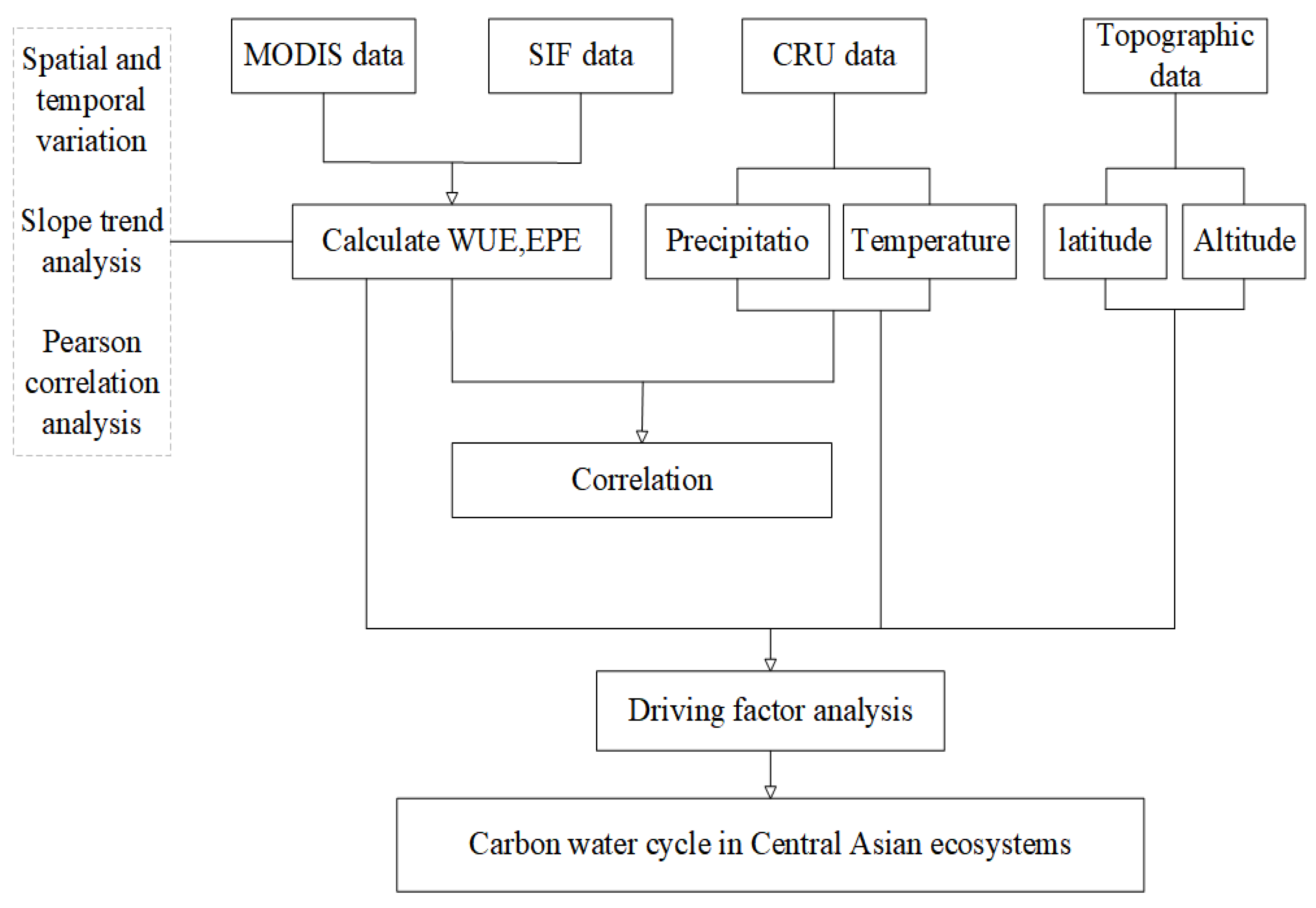
Our analysis was conducted from 2001 to 2020 during the growing season (i.e., from mid-April to early October) because vegetation would be covered with snow in the non-growing season, so satellite sensors would not be able receive vegetation signals, thus affecting the reliability of the data acquired. The MODIS data were preprocessed using the MODIS reprojection tool; this process mainly involved mosaicking images, reprojecting images, and converting the formats of images. From 2001 to 2020, the monthly mean WUE and annual mean WUE were calculated using the average GPP and ET of the 8-day interval in each month; the monthly mean EPE and annual mean EPE were calculated using the average SIF and LAI of the 8 d interval in each month. Variations in the monthly and annual means of WUE and EPE and the spatial distribution of WUE and EPE were analyzed; changes in the slope of the annual mean were also analyzed. The WUE data calculated were resampled by a margin of 0.05° so that they were consistent with the EPE data, and Pearson correlation analysis was conducted to clarify the relationship between WUE and EPE. Data for land cover types that remained stable (i.e., did not change) over the 20-year study period were reclassified, and the WUE and EPE data of the different land cover types were extracted to characterize changes in the WUE and EPE of different vegetation types at different latitudes and altitudes. Finally, the relationships of WUE and EPE with climatic factors were analyzed. Figure 3 presents a flow chart of this study.
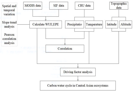
Figure 3.
Research flow chart.
4. Results and Analysis
4.1. Temporal Variation in WUE and EPE
4.1.1. Temporal Variation in WUE
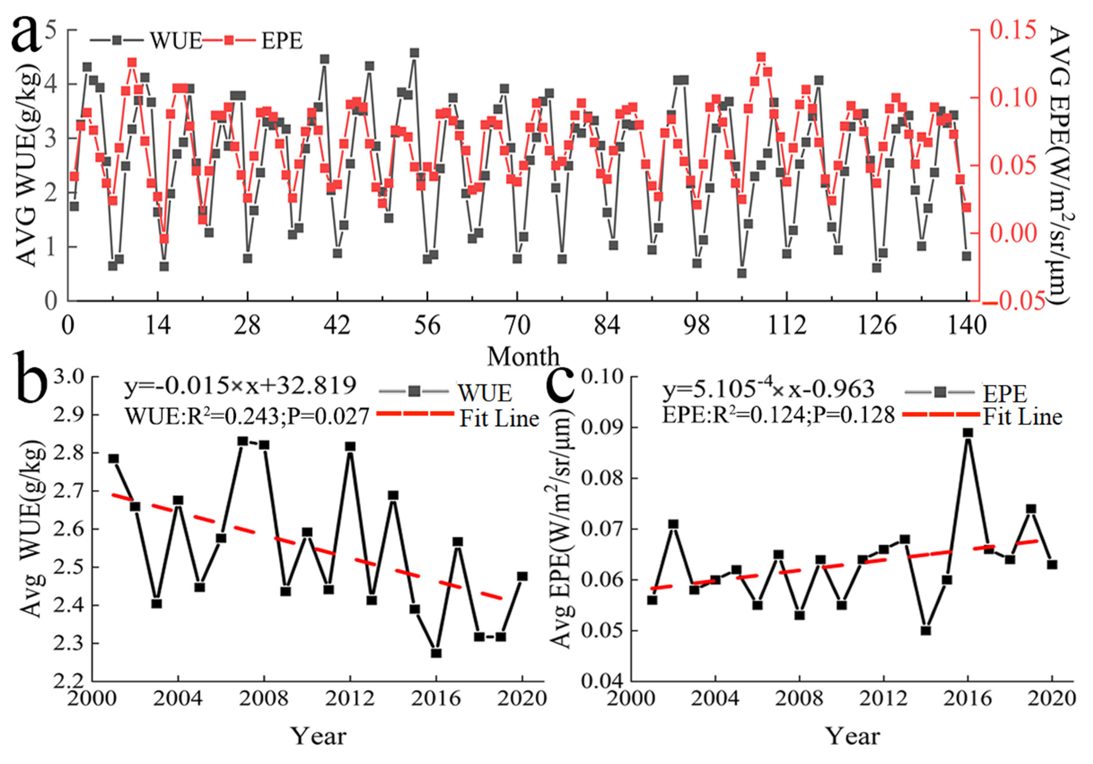
A unimodal pattern was observed in the monthly mean value of WUE in Central Asia (Figure 4a). WUE first increased and then decreased in April, and WUE was highest in August. Vegetation began to decrease in the autumn, and ET will increase in the autumn, so the WUE began to rapidly decrease during this period. Large fluctuations were observed in the annual mean WUE from 2001 to 2020 (Figure 4b). The highest value of WUE was recorded in 2007, and the lowest value was recorded in 2016; there was an overall decrease in WUE over the study period.
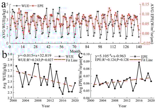
Figure 4.
Temporal variation in WUE and EPE. (a) Monthly mean variation in WUE and EPE (b) and (c) annual mean variation in WUE and EPE.
4.1.2. Temporal Variation in EPE
The pattern in monthly mean EPE in Central Asia was similar to that of WUE. A single peak was observed, and EPE was generally highest in June and July, with this period being followed by a gradual decrease (Figure 4a). The changes in annual mean EPE from 2001 to 2020 were similar to the changes in annual mean WUE (Figure 4c). Large fluctuations in EPE were observed. EPE was lowest in 2014 and highest in 2016; there was an overall increase in EPE over the study period.
4.2. Spatial Variation in WUE and EPE
4.2.1. Spatial Variation in WUE
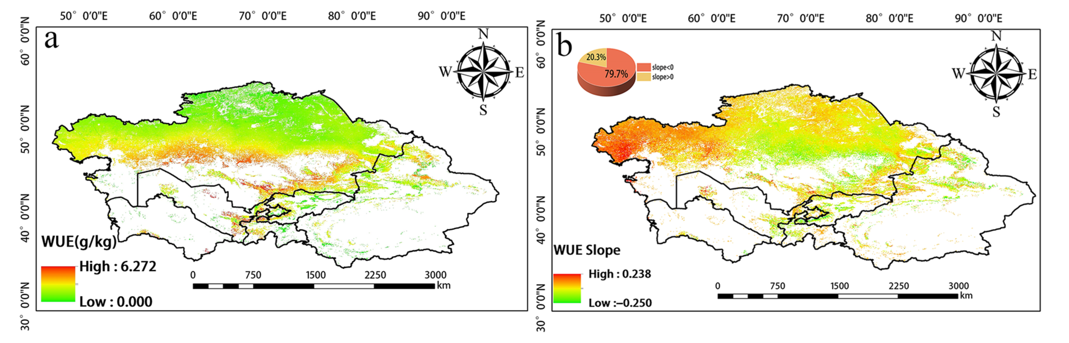
The greatest changes in inter-annual WUE in Central Asia from 2001 to 2020 were observed in the central, western, and southern regions. WUE increased in the western and southern portions of Southern Kazakhstan as well as in the vicinity of Balkhash Lake; WUE slightly decreased around the Taklimakan Desert in the southern part of Xinjiang, China (Figure 5). High WUE was mainly observed in western Tajikistan, eastern Kyrgyzstan, and Southern Kazakhstan, as well as in the Yili, Tacheng, Bortala, and Changji regions of Xinjiang, China. WUE was low in northern Kazakhstan, northern Xinjiang, and Kyrgyzstan (Figure 6a). Changes in WUE over the past 20 years were determined by calculating the slope (Figure 6b). Pixels with a slope less than 0 accounted for 79.7% of the total number of pixels. Pixels with a slope greater than 0 accounted for 20.3% of the total number of pixels. Thus, there was an overall decrease in WUE over this 20-year period.
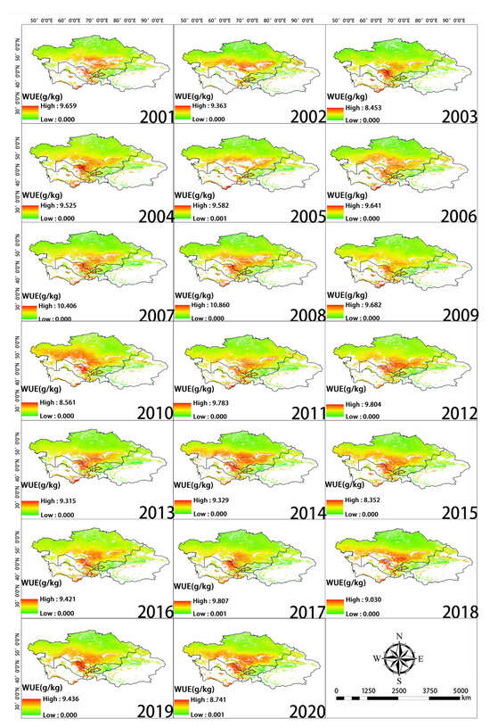
Figure 5.
Spatial distribution of WUE during each year of the study period.
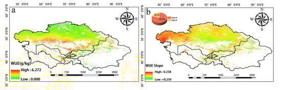
Figure 6.
(a) Spatial distribution of annual mean WUE from 2001 to 2020. (b) Slope of WUE.
4.2.2. Spatial Variation in EPE
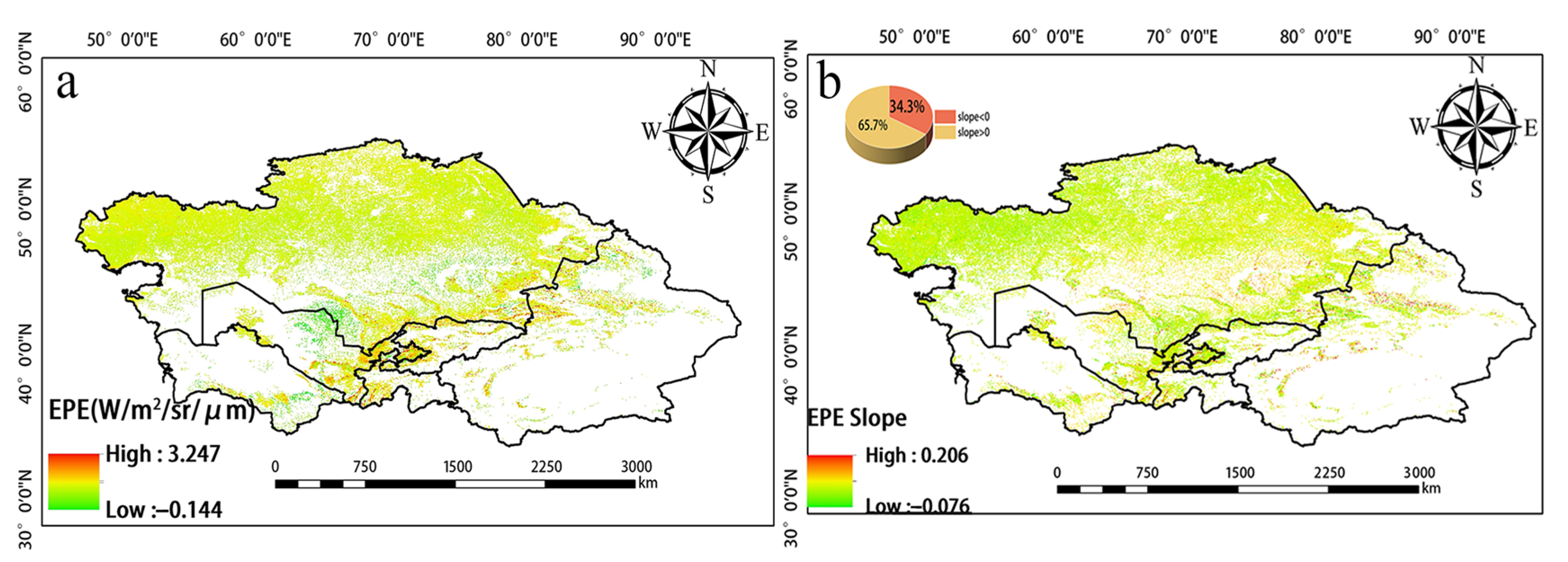
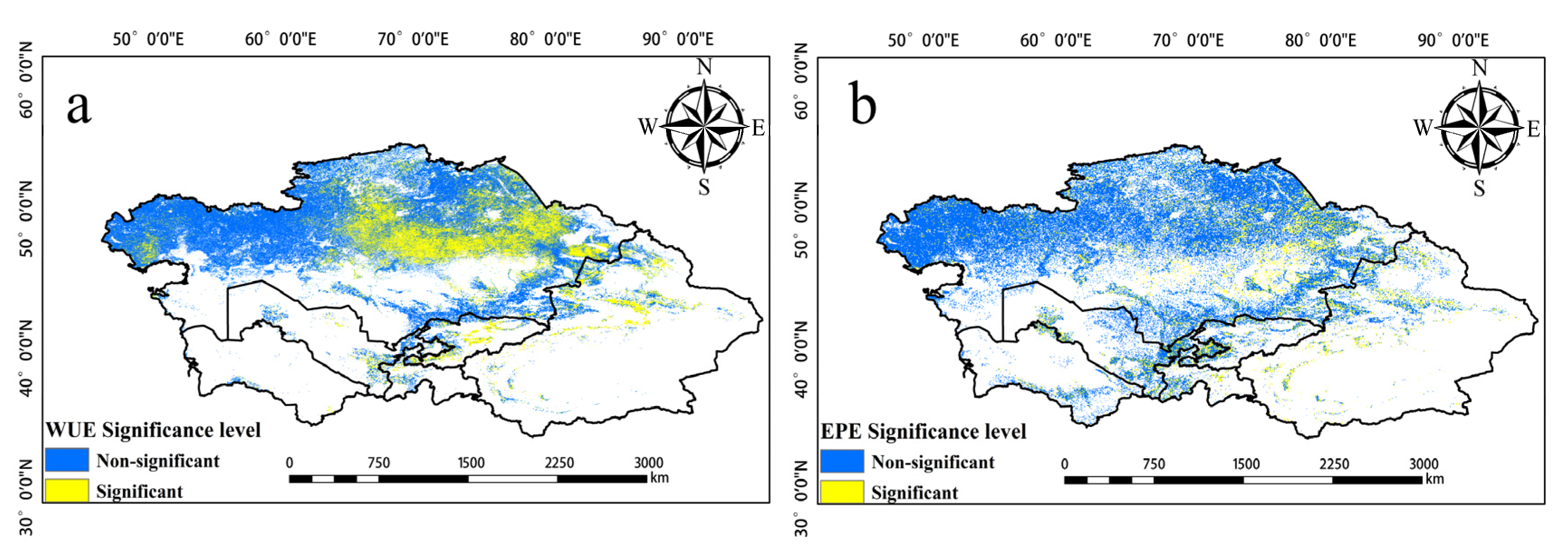
Significant changes in EPE from 2001 to 2020 were observed in the northern, eastern, and southern regions of Central Asia (Figure 7). Over the study period, the EPE in Tajikistan and Uzbekistan increased, and the EPE in Southern Kazakhstan and around Balkhash Lake decreased. High EPE was mainly observed in eastern Uzbekistan, western Tajikistan, Southern Kazakhstan, northern Kyrgyzstan, and the Ili region of Xinjiang, China (Figure 8a). EPE was high in Kyrgyzstan and northern Xinjiang, China, and this was not consistent with the WUE values in these same areas. Changes in EPE over the past 20 years were determined by calculating the slope (Figure 8b). The number of pixels with a slope less than 0 accounted for 34.3% of the total number of pixels. The number of pixels with a slope greater than 0 was 65.7%. Thus, there was an overall increase in EPE over the 20-year period analyzed. Figure 9 provides the level of significance of WUE and EPE.
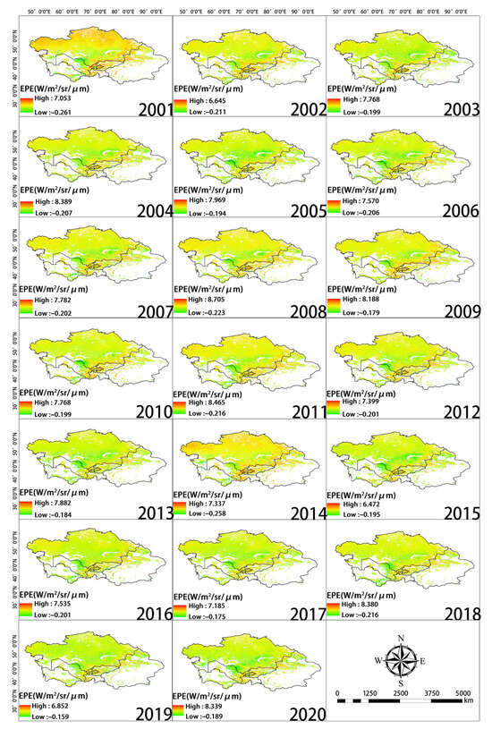
Figure 7.
Spatial distribution of EPE during each year of the study period.

Figure 8.
(a) Spatial distribution of annual mean EPE from 2001 to 2020. (b) Slope of EPE.

Figure 9.
(a) is the significance level of WUE. (b) is the significance level of EPE (α = 0.05).
We used Pearson correlation analysis to analyze correlations between WUE and EPE over the 20-year study period. Negative and positive correlations between WUE and EPE were observed in 73% and 27% of the study area, respectively (Figure 10). Therefore, WUE and EPE were generally negatively correlated.
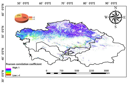
Figure 10.
Correlation between WUE and EPE.
4.3. Variation in WUE and EPE with Altitude and Latitude
4.3.1. Variation in the WUE of Different Types of Vegetation with Altitude and Latitude
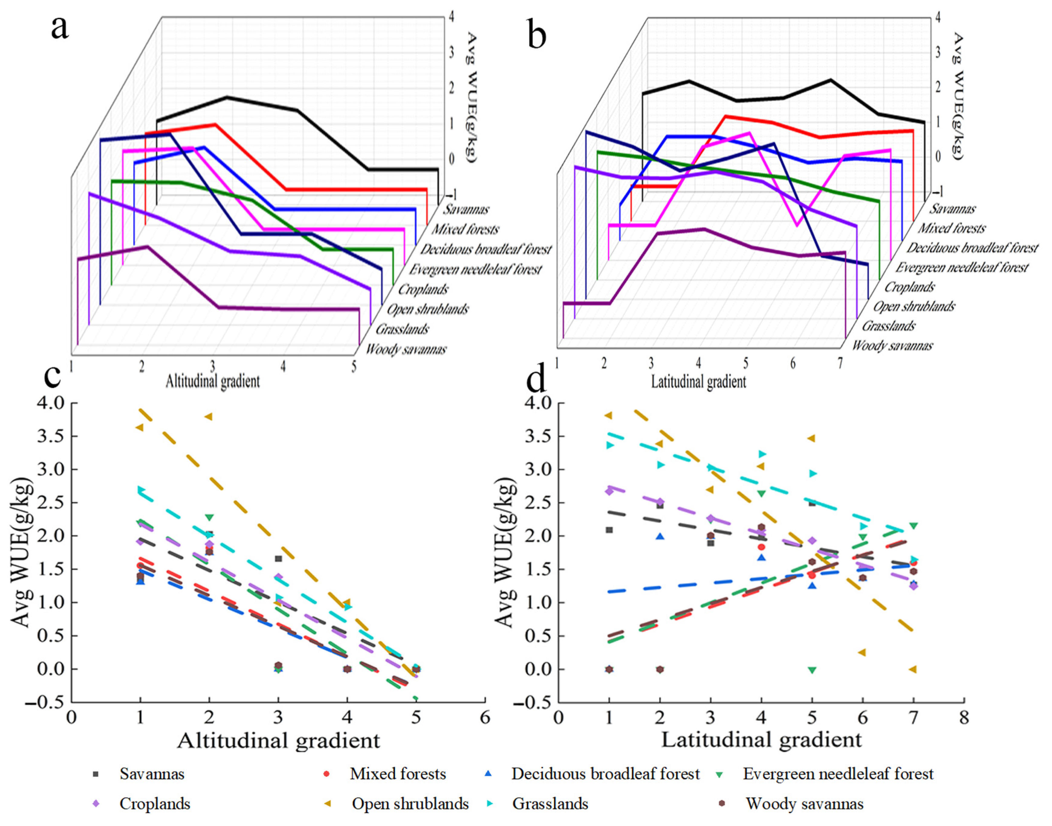
The WUE of savanna increased over altitude bins 1 to 2, decreased over altitude bins 2 to 4, and did not change after altitude bin 4 (Figure 11a). The WUE of mixed forest, deciduous broad-leaved forest, evergreen coniferous forest, and steppes increased over altitude bins 1 to 2, decreased over altitude bins 2 to 3, and did not change after altitude bin 3. The WUE of farmland decreased with altitude and did not change after altitude bin 4. The WUE of open shrubland increased over altitude bins 1 and 2, decreased over altitude bins 2 to 3, and did not change after altitude bin 5. The WUE of grassland also decreased with altitude, and the WUE of grassland did not change after altitude bin 5. Overall, the WUE of all vegetation types decreased with altitude. The WUE of most types of vegetation did not change after altitude bin 3 (Figure 11c).
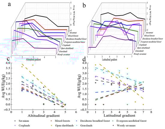
Figure 11.
Variation in the WUE of different vegetation types with altitude and latitude. (a) Relationship between WUE and altitude. (b) Relationship between WUE and latitude. (c) Linear relationship between WUE and altitude. x axis 1: −227–1424; 2: 1424–3075; 3: 3075–4726; 4: 4756–6377; 5: 6377–8028 (m). (d) Linear relationship between WUE and latitude. x axis 1: 30.0–35.6; 2: 35.6–38.3; 3: 38.3–40.9; 4: 40.9–43.5; 5: 43.5–46.1; 6: 46.1–48.8; 7: 48.8–54.0(°). The parameters in Figure 10 are the same.
The WUE of savanna, farmland, open shrubland, and grassland decreased with latitude (Figure 11b). The WUE of mixed forest, deciduous broadleaved forest, evergreen coniferous forest, and steppes increased with latitude. Overall, WUE was lower at higher latitudes (Figure 11d). Table 1 provides their R2 and p.

Table 1.
WUE of different vegetation types and R2 and p values of altitude and latitude under different gradients.
4.3.2. Variation in the EPE of Different Types of Vegetation with Altitude and Latitude
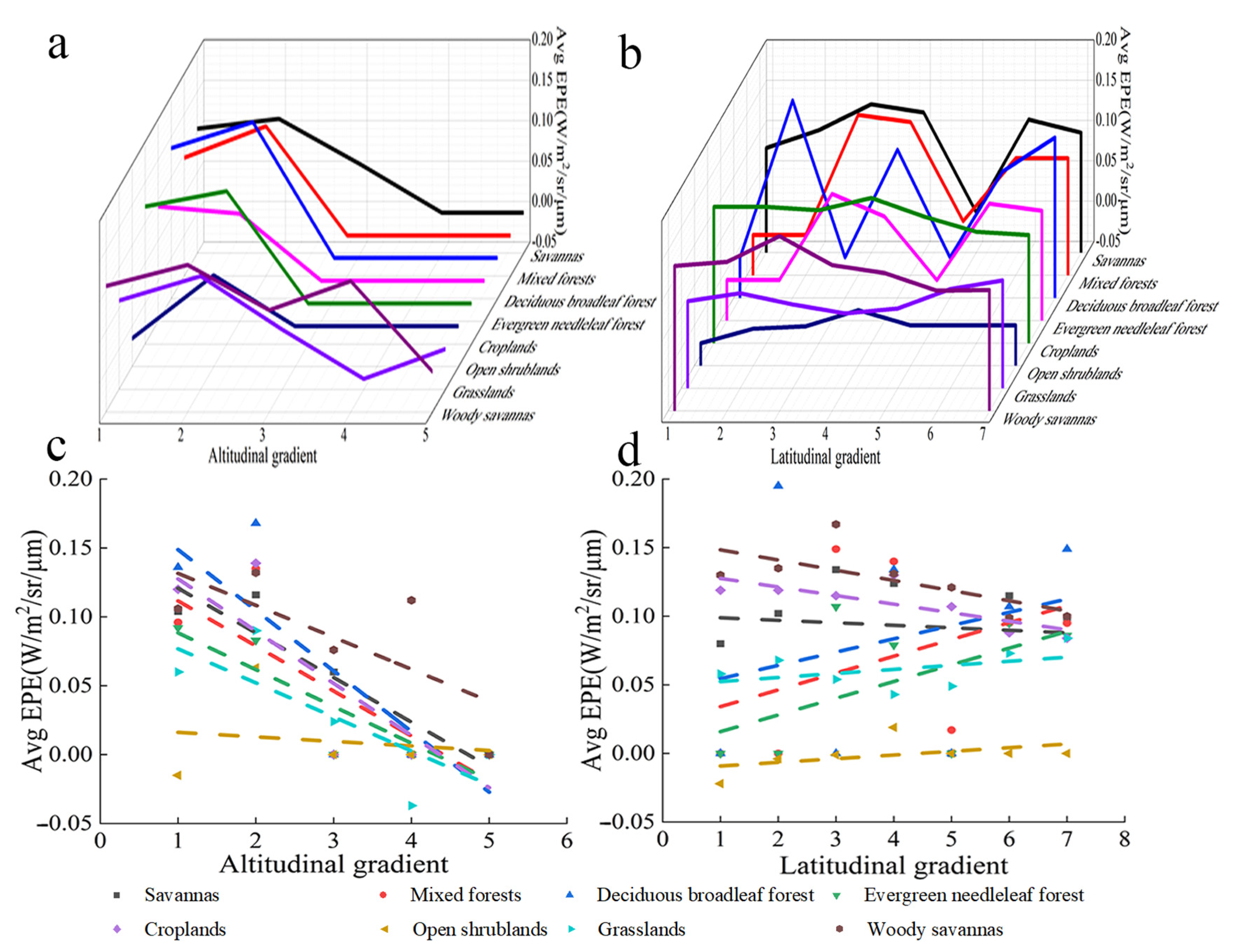
The EPE of savanna increased with altitude; specifically, the EPE of savanna increased over altitude bins 1 to 2, decreased over altitude bins 3 to 4, and did not change after altitude bin 4 (Figure 12a). The EPE of mixed forest, deciduous broadleaved forest, farmland, and open shrubland increased over altitude bins 1 to 2, decreased over altitude bins 2 to 3, and did not change after altitude bin 3. The EPE of evergreen coniferous forest decreased with altitude and did not change after altitude bin 3. The EPE of grassland increased over altitude bins 1 to 2, decreased over altitude bins 3 to 4, and did not change after altitude bin 5. The EPE of multi-tree steppes increased over altitude bins 1 and 2, decreased over altitude bins 2 to 3, increased over altitude bins 3 to 4, decreased over altitude bins 4 to 5, and did not change after altitude bin 5. Overall, the EPE of all types of vegetation decreased with altitude, and the EPE of most types of vegetation did not change after altitude bin 3 (Figure 12c).
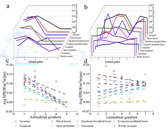
Figure 12.
Variation in the EPE of different types of vegetation with altitude and latitude. (a) Relationship between EPE and altitude. (b) Relationship between EPE and latitude. (c) Linear relationship between EPE and altitude. (d) Linear relationship between EPE and latitude.
The EPE of savanna, farmland, and savannah decreased with latitude (Figure 12b). The EPE of mixed forest, deciduous broadleaved forest, evergreen coniferous forest, open shrubland, and grassland increased with latitude. Overall, the EPE of all vegetation types, with the exception of open shrubland and grassland, decreased with latitude (Figure 12d). Table 2 provides their R2 and p.
Table 2.
EPE of different vegetation types and R2 and p values of elevation and latitude under different gradients.
4.4. Relationships of WUE and EPE with Temperature and Precipitation
4.4.1. Relationship between WUE and Temperature and Precipitation
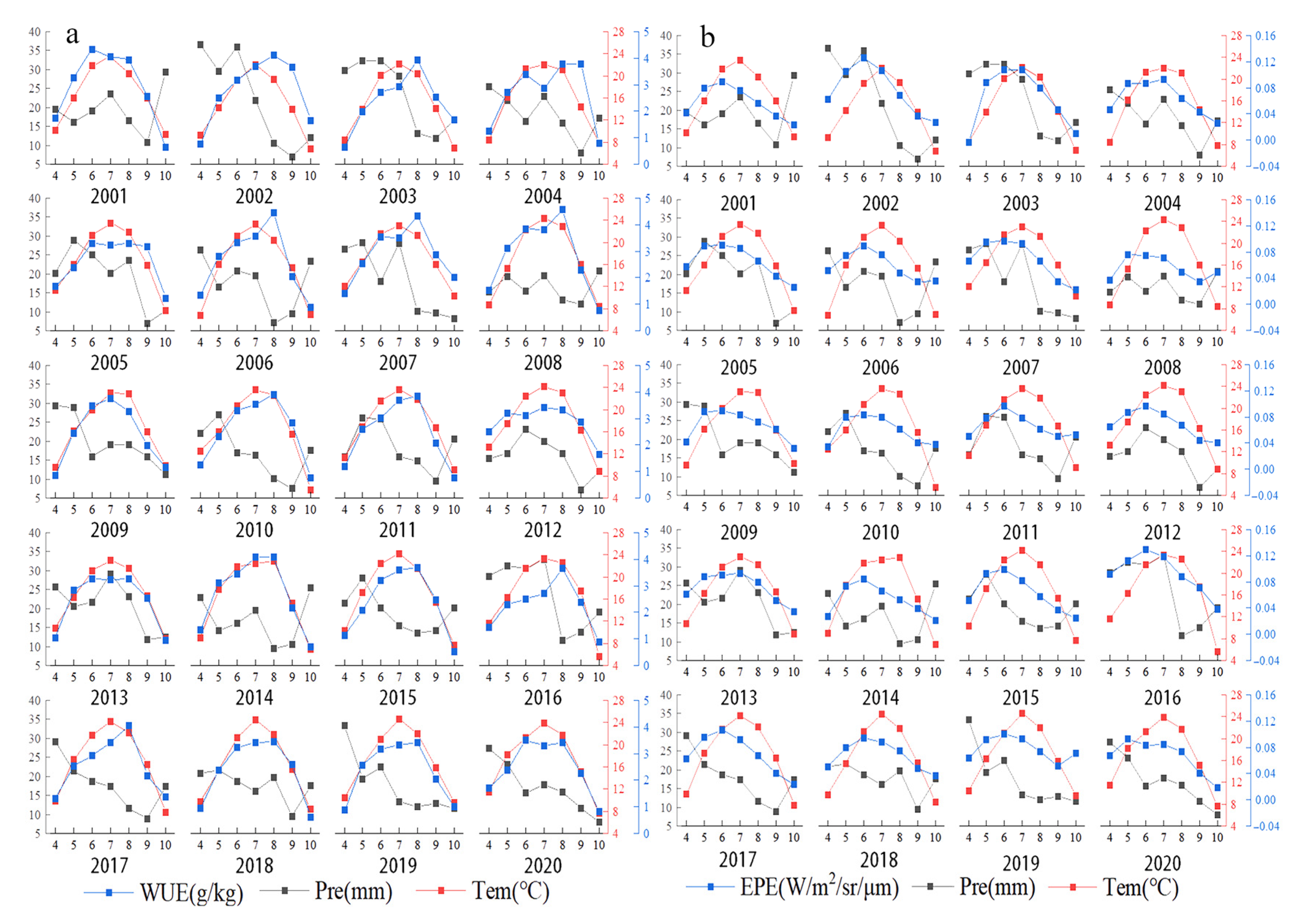
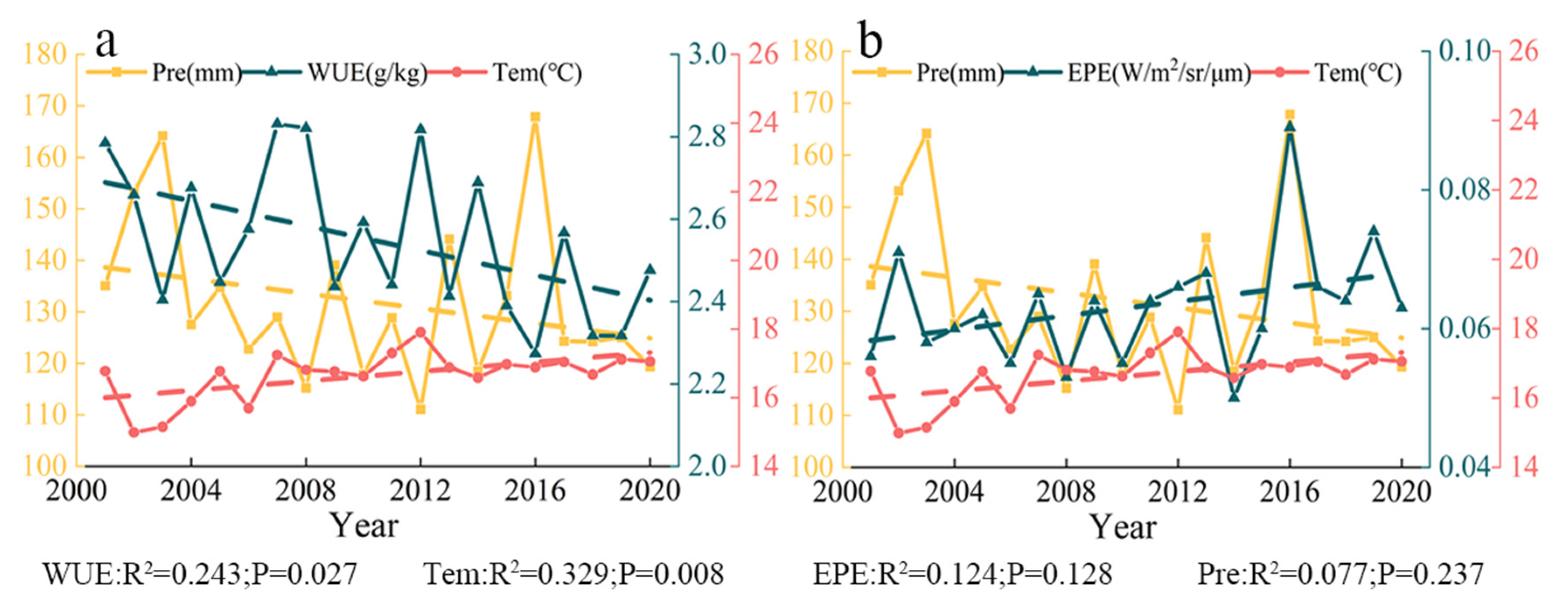
There was an overall positive correlation between the mean WUE and the mean temperature of each month from April to October in Central Asia (Figure 13a). WUE increased with temperature at the monthly scale. The highest monthly mean temperature in Central Asia generally occurs in July, and this is followed by rapid cooling. The mean annual WUE decreased and air temperature increased from 2001 to 2020, which indicated that mean annual WUE and air temperature were negatively correlated at the yearly scale (Figure 14a).
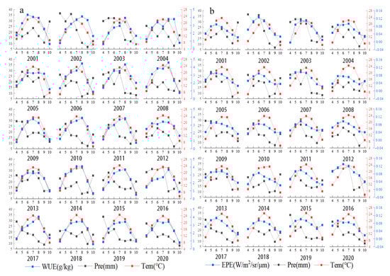
Figure 13.
(a) Monthly mean temperature, precipitation, and WUE in each year from 2001 to 2020. (b) Monthly mean temperature, precipitation, and EPE in each year from 2001 to 2020.
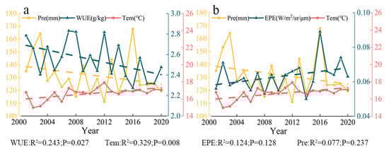
Figure 14.
(a) Annual mean temperature, precipitation amount, and WUE from 2001 to 2020. (b) Annual mean temperature, precipitation amount, and EPE from 2001 to 2020.
There was a negative correlation between the mean monthly WUE and precipitation from April to October; that is, WUE was higher in months when precipitation was lower (Figure 13a). Mean annual WUE and precipitation amount decreased over the 20-year study period; mean annual WUE and annual precipitation were thus positively correlated at the yearly scale (Figure 14a). WUE was high in 2007, 2008, and 2012, but the amount of precipitation in these years was not very high.
4.4.2. Relationship between EPE and Temperature and Precipitation
There was a positive correlation between the mean EPE and mean temperature of each month from April to October, and EPE increased with temperature (Figure 13b). Across the 20-year study period, the mean annual EPE and temperature increased; they were thus positively correlated at the yearly scale (Figure 14b).
There was a positive correlation between the mean monthly EPE and precipitation from April to October (Figure 13b). Throughout the 20-year study period, mean annual EPE increased, and annual precipitation decreased; EPE and annual precipitation were thus negatively correlated at the yearly scale (Figure 14b). The EPE value in 2016 was the highest, and the precipitation value at this time was also the highest.
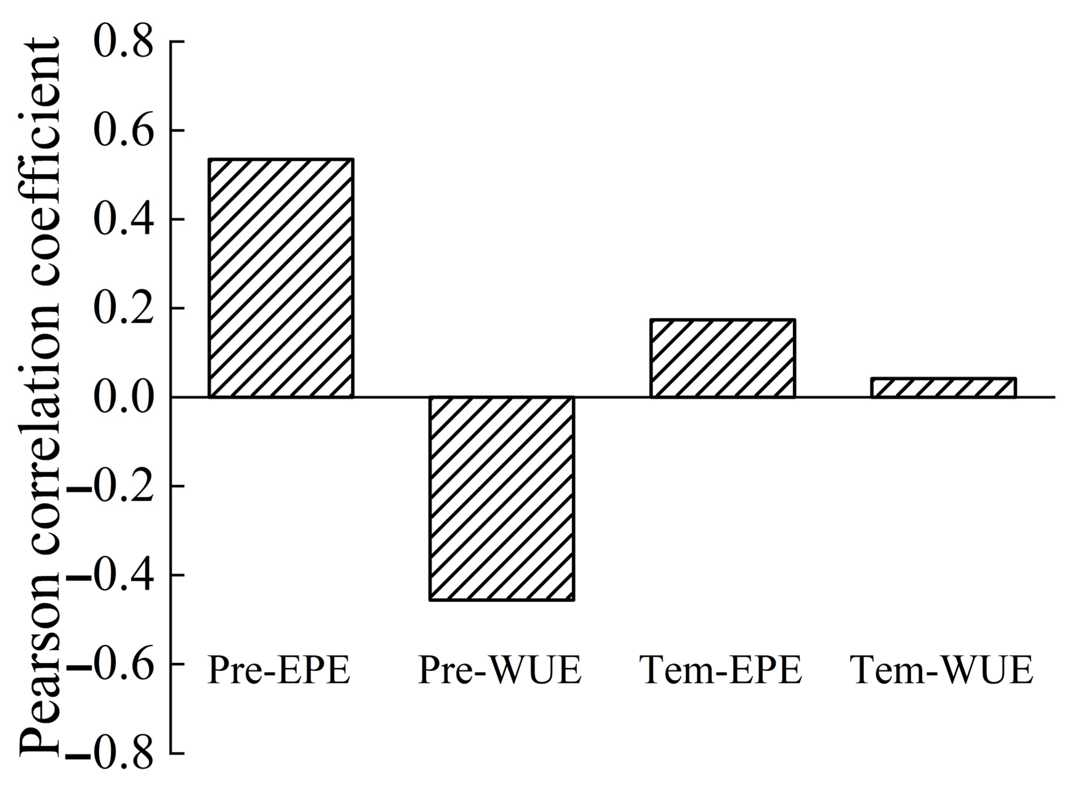
The correlation coefficients for the precipitation–EPE, precipitation–WUE, temperature–EPE, and temperature–WUE correlations at the yearly scale were 0.535 (p = 0.015), −0.456 (p = 0.043), 0.174 (p = 0.463), and 0.042 (p = 0.042), respectively (Figure 15). All these correlations were positive, with the exception of a negative correlation between precipitation and WUE. The correlation between precipitation and EPE was the strongest, and the correlation between temperature and WUE was the weakest.
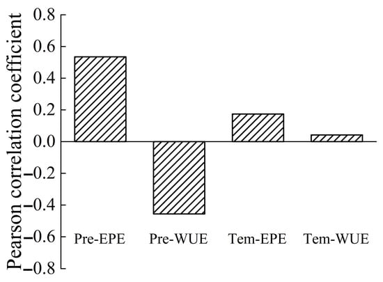
Figure 15.
Correlations of WUE and EPE with precipitation and temperature at the yearly scale.
5. Discussion
5.1. Limitations of the Study and Reliability of the Data
Remote-sensing satellite data have various advantages, including the large scale at which these data can be continuously collected; however, several factors, such as climatic conditions, can affect the quality of remote-sensing data. Several uncertainties in the remote-sensing data obtained in this study require consideration. For example, the remote-sensing data do not account for the effects of environmental factors, anthropogenic disturbance, and other factors. However, bare land with sparse vegetation cover was excluded from our analyses, and this increased the robustness of our results. GPP and ET data were used to calculate WUE; SIF and LAI data were used to calculate EPE; and the effects of CRU, MOD12Q1, DEM, and other types of data on WUE and EPE were examined. Several experimental studies have been conducted to assess the accuracy and applicability of the above data [4,17,23], and these studies have suggested that these data are sufficiently reliable to be of use in practical applications. However, due to the lack of verification of ground observation or independent datasets, the above data still have some limitations, which introduced some uncertainties in this study.
5.2. Temporal Variation in WUE and EPE
Mean WUE and EPE were analyzed at the monthly and annual scales in Central Asia. The patterns of mean monthly WUE and EPE were unimodal. Large fluctuations in WUE and EPE and multiple peaks of WUE and EPE were observed at the yearly scale. Zhu et al. examined seasonal changes in the WUE of typical forest and grassland ecosystems in China and found that several environmental and biological factors associated with drought are responsible for the bimodal or multi-peak patterns in WUE in dry years [58]. This conclusion is consistent with the results of our study. We found that inter-monthly WUE and EPE in Central Asia first increased and then decreased over the growing season, and this behavior was related to seasonal changes, anthropogenic disturbance, and other factors. Variation in interannual WUE in arid ecosystems is consistent with variation in GPP. Therefore, WUE is higher in years with high GPP [59,60,61,62,63]. Over long time scales, the WUE of regional ecosystems increases or decreases depending on changes in environmental conditions [64]. In our study, WUE decreased and EPE increased from 2001 to 2020.
5.3. Spatial Variation in WUE and EPE at the Yearly Scale
Tian et al. observed significant spatial variation in WUE [65]. In our study, WUE was high in the western and southern portions of Southern Kazakhstan as well as in the vicinity of Balkhash Lake; WUE was low around Taklimakan in southern Xinjiang, China. These findings are consistent with the results reported by Zou et al. [1]. Regions with high WUE and EPE and low WUE and EPE were observed; however, some regions with high WUE had low EPE. There was large spatial heterogeneity in WUE and EPE, and there are several potential explanations for this spatial heterogeneity. The responses of WUE and EPE to arid climates differ; in fact, the lack of precipitation results in drought and higher evaporative demand due to air dryness (high VPD), increasing ET [66,67]. Usually, at the beginning of a water deficit, plants close their stomata, so stomatal conductance and ET decrease at a higher rate than GPP, thus increasing WUE [68]; from another point of view, water stress is high when GPP is decreased to a level where WUE can be decreased [69,70]. Studies have shown that Central Asia experienced a severe drought in 2008, with high water stress and a rapid decline in WUE [71], and this finding is consistent with the results of this study. In arid areas, increases in light intensity can lead to increases in EPE. In addition, natural factors, such as drought, soil moisture, VPD, and CO2 levels, and anthropogenic factors, such as grazing [72] and habitat degradation, can explain spatial heterogeneity in WUE and EPE. All of the above factors can lead to environmental changes that affect WUE and EPE; thus, the relationship between WUE and EPE is complex and dynamic. Several studies have shown that drought is negatively correlated with WUE and positively correlated with EPE. Therefore, heterogeneity in the spatial distribution of drought and WUE might be related to arid climatic conditions.
5.4. Relationship between WUE and EPE
WUE and EPE were negatively correlated according to Pearson correlation analysis. EPE was highest in June and July, and WUE was highest in August (Figure 3a). We speculate that plants first use light and then reuse water in the growth process. Chung et al. [73] noted that photoinduced stomatal responses can enhance the drought tolerance of plants [74], and the water stress of plants is temperature-dependent [75]. Thus, increases in photosynthetic efficiency might be one of the main reasons for the increases in ecosystem productivity in arid environments. In our study, the effects of the drought index on these two factors were not examined. The results of previous studies indicate that WUE decreases in arid climates [76,77,78,79]. However, EPE increases with the intensity of drought [23]. Thus, we concluded that the intensity of drought was positively correlated with EPE and negatively correlated with WUE. Additional studies are needed to verify these assumptions.
5.5. Variation in the WUE and EPE of Different Types of Vegetation with Altitude and Latitude
Gang et al. noted that approximately 39.76% of grassland areas in the world were in a state of drought from 2000 to 2011 [80]. Zhu et al. showed that WUE decreases significantly with altitude, and they argued that this pattern is related to the distribution of ecosystem types associated with altitudinal variation in climate [15]. Xue et al. found that WUE varies with latitude [44]. We found that patterns of variation in WUE and EPE varied with altitude and latitude. The growth of vegetation tends to be constrained at higher altitudes. Consequently, WUE and EPE tended toward zero at high altitudes. Climatic zones vary with latitude, and the WUE and EPE of different types of vegetation decreased from south to north.
5.6. Relationship of WUE and EPE with Temperature and Precipitation
Xue et al. examined patterns in WUE on a global scale from 2000 to 2013, as well as the factors driving these patterns, and found that WUE is negatively correlated with temperature and solar radiation [44]. However, Zhou et al. showed that WUE is positively correlated with temperature [81]. We found that WUE and temperature were weakly positively correlated from 2001 to 2020, and this was related to spatial and temporal differences in vegetation and climatic characteristics. At high temperatures, the rate of increase in ET is much higher than that of GPP [10]; consequently, WUE decreases as temperature increases [82]. At the monthly scale, WUE was positively correlated with temperature, and WUE was highest in the summer; adequate WUE can also maximize the absorption and conversion of water during the summer when plants are growing and flourishing. Temperature and EPE were negatively correlated from 2001 to 2009 and positively correlated from 2010 to 2020. The temperature was higher in July and August than in May and June, but EPE was lower in July and August than in May and June; this was not only related to the abundance of light but also to LAI. Light is abundant in July and August, and LAI is stable during this period. In addition, high temperatures can inhibit the photosynthesis of plants [83]. SIF and LAI differ among different plants, and this is not only related to the chlorophyll content and photosynthetic capacity of leaves but also to the amount of sunshine; temperature can have a major effect on the photosynthetic activity of plants. Temperature is thus an important determinant of the global carbon balance [84,85]; the relationship between EPE and temperature should be positive. WUE and precipitation have been shown to be negatively correlated in many studies [86]. Yang et al. examined the effects of different factors on changes in WUE in Northwest China and found that the contribution of precipitation to increases in WUE is as high as 66%, whereas that of temperature is 12% [87]; these findings are consistent with the results of our study.
6. Conclusions
We used remote-sensing data and geographic information system technology to analyze spatial and temporal variations in WUE and EPE in Central Asia from 2001 to 2020 as well as the relationships of WUE and EPE with precipitation and temperature. At the monthly scale, variation in WUE and EPE was unimodal, and EPE and WUE were highest in June–July and August, respectively. From 2001 to 2020, WUE decreased, and EPE increased. There was a high degree of spatial heterogeneity in WUE and EPE. WUE and EPE were negatively correlated. WUE and EPE decreased with altitude, and the WUE and EPE values of most types of vegetation were zero after the 3075–4276 m altitude bin. The WUE and EPE of the different types of vegetation decreased with latitude. From 2001 to 2020, precipitation was the main factor affecting variation in WUE, and temperature was the main factor affecting variation in EPE. We analyzed temporal and spatial variation in WUE and EPE. Our findings provide valuable information that will aid future studies on the carbon–water cycle in Central Asia and provide guidance on regional water management and land use planning. However, in this study, we did not carry out field verification, so the data had certain limitations, and other driving factors were not analyzed, such as drought index, soil moisture, photosynthetically active radiation, etc. In future studies, we will examine the data and fully consider the influences of various factors on water resource use efficiency and ecosystem-scale photosynthetic efficiency.
Author Contributions
J.Z. and H.Y. conceived and designed this study, H.Y. carried out the analyses and wrote the paper; J.D. and W.Z. contributed to the discussion and manuscript refinement. W.T. and M.Y. made important contributions to the figures. All authors have read and agreed to the published version of the manuscript.
Funding
This work was supported by the National Natural Science Foundation of China (Nos. 32260287 and 41961059), the Doctoral Research Start-up Fund Project of Xinjiang University (No. 620320025), the Sino-German interdisciplinary joint program for innovative talent training funded by the China Scholarship Council (CSC, No. 201807015008), and The Technology Innovation Team (Tianshan Innovation Team), Innovative Team for Efficient Utilization of Water Resources in Arid Regions (No. 2022TSYCTD0001).
Data Availability Statement
The data used in this study are available in the Methods.
Conflicts of Interest
The authors declare no conflict of interest.
References
- Zou, J.; Ding, J.; Welp, M.; Huang, S.; Liu, B. Using MODIS data to analyse the ecosystem water use efficiency spatial-temporal variations across Central Asia from 2000 to 2014. Environ. Res. 2020, 182, 108985. [Google Scholar] [CrossRef] [PubMed]
- Ciais, P.; Reichstein, M.; Viovy, N.; Granier, A.; Ogée, J.; Allard, V.; Aubinet, M.; Buchmann, N.; Bernhofer, C.; Carrara, A.; et al. Europe-wide reduction in primary productivity caused by the heat and drought in 2003. Nature 2005, 437, 529–533. [Google Scholar] [CrossRef]
- Hicke, J.A.; Allen, C.D.; Desai, A.R.; Dietze, M.C.; Hall, R.J.; Hogg, E.H.; Kashian, D.M.; Moore, D.J.; Raffa, K.F.; Sturrock, R.N.; et al. Effects of biotic disturbances on forest carbon cycling in the United States and Canada. Glob. Chang. Biol. 2012, 18, 7–34. [Google Scholar] [CrossRef]
- Tang, X.; Li, H.; Desai, A.R.; Nagy, Z.; Luo, J.; Kolb, T.E.; Olioso, A.; Xu, X.; Yao, L.; Kutsch, W.; et al. How is water-use efficiency of terrestrial ecosystems distributed and changing on Earth? Sci. Rep. 2014, 4, 7483. [Google Scholar] [CrossRef]
- Westerling, A.L.; Hidalgo, H.G.; Cayan, D.R.; Swetnam, T.W. Warming and earlier spring increase western, U.S. forest wildfire activity. Science 2006, 313, 940–943. [Google Scholar] [CrossRef] [PubMed]
- Sun, Y.; Piao, S.; Huang, M.; Ciais, P.; Zeng, Z.; Cheng, L.; Li, X.; Zhang, X.; Mao, J.; Peng, S.; et al. Global patterns and climate drivers of water-use efficiency in terrestrial ecosystems deduced from satellite-based datasets and carbon cycle models. Glob. Ecol. Biogeogr. 2016, 25, 311–323. [Google Scholar] [CrossRef]
- Guerrieri, R.; Lepine, L.; Asbjornsen, H.; Xiao, J.; Ollinger, S.V. Evapotranspiration and water use efficiency in relation to climate and canopy nitrogen in U.S. forests. J. Geophys. Res. Biogeosciences 2016, 121, 2610–2629. [Google Scholar] [CrossRef]
- Frank, D.C.; Poulter, B.; Saurer, M.; Esper, J.; Huntingford, C.; Helle, G.; Treydte, K.; Zimmermann, N.E.; Schleser, G.H.; Ahlström, A.; et al. Water-use efficiency and transpiration across European forests during the Anthropocene. Nat. Clim. Chang. 2015, 5, 579–583. [Google Scholar] [CrossRef]
- Zhou, S.; Yu, B.; Schwalm, C.R.; Ciais, P.; Zhang, Y.; Fisher, J.B.; Michalak, A.M.; Wang, W.; Poulter, B.; Huntzinger, D.N. Response of water use efficiency to global environmental change based on output from terrestrial bio-sphere models. Earth Sustain. 2017, 31, 1639–1655. [Google Scholar]
- Yu, G.; Song, X.; Wang, Q.; Liu, Y.; Guan, D.; Yan, J.; Sun, X.; Zhang, L.; Wen, X.J. Water-use efficiency of forest eco-systems in eastern China and its relations to climatic variables. New Phytol. 2008, 177, 927–937. [Google Scholar] [CrossRef]
- Tong, X.; Zhang, J.; Meng, P.; Li, J.; Zheng, N. Ecosystem water use efficiency in a warm-temperate mixed plantation in the North China. J. Hydrol. 2014, 512, 221–228. [Google Scholar] [CrossRef]
- Lin, Y.; Grace, J.; Zhao, W.; Dong, Y.; Zhang, X.; Zhou, L.; Fei, X.; Jin, Y.; Li, J.; Nizami, S.M.; et al. Water-use efficiency and its relationship with environmental and biological factors in a rubber plantation. J. Hydrol. 2018, 563, 273–282. [Google Scholar] [CrossRef]
- Zhu, Q.; Jiang, H.; Peng, C.; Liu, J.; Wei, X.; Fang, X.; Liu, S.; Zhou, G.; Yu, S. Evaluating the effects of future climate change and elevated CO2 on the water use efficiency in terrestrial ecosystems of China. Ecol. Model. 2011, 222, 2414–2429. [Google Scholar] [CrossRef]
- Gao, Y.; Zhu, X.J.; Yu, G.R.; He, N.P.; Wang, Q.F.; Tian, J. Water use efficiency threshold for terrestrial ecosystem carbon sequestration in China under afforestation. Agric. For. Meteorol. 2014, 195, 32. [Google Scholar]
- Zhu, X.-J.; Yu, G.-R.; Wang, Q.-F.; Hu, Z.-M.; Zheng, H.; Li, S.-G.; Sun, X.-M.; Zhang, Y.-P.; Yan, J.-H.; Wang, H.-M.; et al. Spatial variability of water use efficiency in China’s terrestrial ecosystems. Glob. Planet. Chang. 2015, 129, 37–44. [Google Scholar] [CrossRef]
- Sun, S.; Song, Z.; Wu, X.; Wang, T.; Wu, Y.; Du, W.; Che, T.; Huang, C.; Zhang, X.; Ping, B.; et al. Spatiotemporal variations in water use efficiency and its drivers in China over the last three decades. Ecol. Indic. 2018, 94, 292–304. [Google Scholar] [CrossRef]
- Li, X.; Xiao, J. A Global, 0.05-Degree Product of Solar-Induced Chlorophyll Fluorescence Derived from OCO-2, MODIS, and Reanalysis Data. Remote Sens. 2019, 11, 517. [Google Scholar] [CrossRef]
- Joiner, J.; Yoshida, Y.; Kehler, P.; Campbell, P.; Sun, Y.J. Systematic Orbital Geometry-Dependent Variations in Satellite Solar-Induced Fluorescence (SIF) Retrievals. Remote Sens. 2020, 12, 2346. [Google Scholar] [CrossRef]
- Sun, Y.; Frankenberg, C.; Wood, J.D.; Schimel, D.S.; Jung, M.; Guanter, L.; Drewry, D.T.; Verma, M.; Porcar-Castell, A.; Griffis, T.J.; et al. OCO-2 advances photosynthesis observation from space via solar-induced chlorophyll fluorescence. Science 2017, 358, eaam5747. [Google Scholar] [CrossRef]
- Sun, Y.; Frankenberg, C.; Jung, M.; Joiner, J.; Guanter, L.; Köhler, P.; Magney, T. Overview of Solar-Induced chlorophyll Fluorescence (SIF) from the Orbiting Carbon Observatory-2: Retrieval, cross-mission comparison, and global monitoring for GPP. Remote Sens. Environ. 2018, 209, 808–823. [Google Scholar] [CrossRef]
- Xiao, J.; Li, X.; He, B.; Arain, M.A.; Beringer, J.; Desai, A.R.; Emmel, C.; Hollinger, D.Y.; Krasnova, A.; Mammarella, I.; et al. Solar-induced chlorophyll fluorescence exhibits a universal relationship with gross primary productivity across a wide variety of biomes. Glob. Chang. Biol. 2019, 25, E4–E6. [Google Scholar] [CrossRef]
- Mohammed, G.H.; Colombo, R.; Middleton, E.M.; Rascher, U.; van der Tol, C.; Nedbal, L.; Goulas, Y.; Pérez-Priego, O.; Damm, A.; Meroni, M.; et al. Remote sensing of solar-induced chlorophyll fluorescence (SIF) in vegetation: 50 years of progress. Remote. Sens. Environ. 2019, 231, 111177. [Google Scholar] [CrossRef]
- Wei, F.; Wang, S.; Fu, B.; Wang, L.; Zhang, W.; Wang, L.; Pan, N.; Fensholt, R. Divergent trends of ecosystem-scale photosynthetic efficiency between arid and humid lands across the globe. Glob. Ecol. Biogeogr. 2022, 31, 1824–1837. [Google Scholar] [CrossRef]
- Zhang, Y.; Tariq, A.; Hughes, A.C.; Hong, D.; Wei, F.; Sun, H.; Sardans, J.; Peñuelas, J.; Perry, G.; Qiao, J.; et al. Challenges and solutions to biodiversity conservation in arid lands. Sci. Total Environ. 2022, 857, 159695. [Google Scholar] [CrossRef] [PubMed]
- Papanatsiou, M.; Petersen, J.; Henderson, L.; Wang, Y.; Christie, J.M.; Blatt, M.R. Optogenetic manipulation of stomatal kinetics improves carbon assimilation, water use, and growth. Science 2019, 363, 1456–1459. [Google Scholar] [CrossRef] [PubMed]
- Jasechko, S.; Sharp, Z.D.; Gibson, J.J.; Birks, S.J.; Yi, Y.; Fawcett, P.J. Terrestrial water fluxes dominated by transpiration. Nature 2013, 496, 347–350. [Google Scholar] [CrossRef] [PubMed]
- Xiao, J.; Xie, B.; Zhou, K.; Li, J.; Xie, J.; Liang, C.J. Contributions of Climate Change, Vegetation Growth, and Elevat-ed Atmospheric CO2 Concentration to Variation in Water Use Efficiency in Subtropical China. Remote Sens. 2022, 14, 4296. [Google Scholar] [CrossRef]
- Poulter, B.; Frank, D.; Ciais, P.; Myneni, R.B.; Andela, N.; Bi, J.; Broquet, G.; Canadell, J.G.; Chevallier, F.; Liu, Y.Y.; et al. Contribution of semi-arid ecosystems to interannual variability of the global carbon cycle. Nature 2014, 509, 600–603. [Google Scholar] [CrossRef]
- Niu, S.; Xing, X.; Zhang, Z.; Xia, J.; Zhou, X.; Song, B.; Li, L.; Wan, S. Water-use efficiency in response to climate change: From leaf to ecosystem in a temperate steppe. Glob. Chang. Biol. 2011, 17, 1073–1082. [Google Scholar] [CrossRef]
- Zou, J.; Ding, J.; Huang, S.; Liu, B. Ecosystem Resistance and Resilience after Dry and Wet Events across Central Asia Based on Remote Sensing Data. Remote Sens. 2023, 15, 3165. [Google Scholar] [CrossRef]
- Peng, D.; Zhou, T.; Zhang, L.; Zhang, W.; Chen, X. Observationally constrained projection of the reduced intensification of extreme climate events in Central Asia from 0.5 °C less global warming. Clim. Dyn. 2020, 54, 543–560. [Google Scholar] [CrossRef]
- Hu, Z.; Zhou, Q.; Chen, X.; Qian, C.; Wang, S.; Li, J. Variations and changes of annual precipitation in Central Asia over the last century. Int. J. Clim. 2017, 37, 157–170. [Google Scholar] [CrossRef]
- Huang, J.; Ji, M.; Xie, Y.; Wang, S.; He, Y.; Ran, J. Global semi-arid climate change over last 60 years. Clim. Dyn. 2016, 46, 1131–1150. [Google Scholar] [CrossRef]
- Liu, L.; Peng, J.; Li, G.; Guan, J.; Han, W.; Ju, X.; Zheng, J. Effects of drought and climate factors on vegetation dynamics in Central Asia from 1982 to 2020. J. Environ. Manag. 2023, 328, 116997. [Google Scholar] [CrossRef]
- Li, Z.; Chen, Y.; Fang, G.; Li, Y. Multivariate assessment and attribution of droughts in Central Asia. Sci. Rep. 2017, 7, 1316. [Google Scholar] [CrossRef] [PubMed]
- Hu, R.; Jiang, F.; Wang, Y.; Li, J.; Li, Y.; Abdimijit, A.; Luo, G.; Zhang, J. Arid Ecological and Geographical Conditions in Five Countries of Central Asia. Arid. Zone Res. 2014, 31, 1–12. [Google Scholar]
- Deng, H.; Chen, Y. Influences of recent climate change and human activities on water storage variations in Central Asia. J. Hydrol. 2017, 544, 46–57. [Google Scholar] [CrossRef]
- Zou, J.; Ding, J. Changes of Water Use Efficiency of Main Vegetation Types in Central Asia from 2000 to 2014. Sci. Silvae Sin. 2019, 55, 175–182. [Google Scholar]
- Kariyeva, J.; van Leeuwen, W.J. Phenological dynamics of irrigated and natural drylands in Central Asia before and after the USSR collapse. Agric. Ecosyst. Environ. 2012, 162, 77–89. [Google Scholar] [CrossRef]
- Mohammat, A.; Wang, X.; Xu, X.; Peng, L.; Yang, Y.; Zhang, X.; Myneni, R.B.; Piao, S. Drought and spring cooling induced recent decrease in vegetation growth in Inner Asia. Agric. For. Meteorol. 2013, 178, 21–30. [Google Scholar] [CrossRef]
- Cao, H.; Gao, B.; Gong, T.; Wang, B. Analyzing Changes in Frozen Soil in the Source Region of the Yellow River Using the MODIS Land Surface Temperature Products. Remote Sens. 2021, 13, 180. [Google Scholar] [CrossRef]
- Khalid, B.; Khalid, A.; Muslim, S.; Habib, A.; Khan, K.; Alvim, D.S.; Shakoor, S.; Mustafa, S.; Zaheer, S.; Zoon, M.; et al. Estimation of aerosol optical depth in relation to meteorological parameters over eastern and western routes of China Pakistan economic corridor. J. Environ. Sci. 2021, 99, 28–39. [Google Scholar] [CrossRef]
- Heinsch, F.; Zhao, M.; Running, S.; Kimball, J.; Nemani, R.; Davis, K.; Bolstad, P.; Cook, B.; Desai, A.; Ricciuto, D.; et al. Evaluation of remote sensing based terrestrial productivity from MODIS using regional tower eddy flux network observations. IEEE Trans. Geosci. Remote Sens. 2006, 44, 1908–1925. [Google Scholar] [CrossRef]
- Xue, B.-L.; Guo, Q.; Otto, A.; Xiao, J.; Tao, S.; Li, L. Global patterns, trends, and drivers of water use efficiency from 2000 to 2013. Ecosphere 2015, 6, 1–18. [Google Scholar] [CrossRef]
- Turner, D.P.; Ritts, W.D.; Cohen, W.B.; Gower, S.T.; Running, S.W.; Zhao, M.; Costa, M.H.; Kirschbaum, A.A.; Ham, J.M.; Saleska, S.R.; et al. Evaluation of MODIS NPP and GPP products across multiple biomes. Remote Sens. Environ. 2006, 102, 282–292. [Google Scholar] [CrossRef]
- Forzieri, G.; Alkama, R.; Miralles, D.G.; Cescatti, A. Satellites reveal contrasting responses of regional climate to the widespread greening of Earth. Science 2017, 356, 1140–1144. [Google Scholar] [CrossRef]
- Gang, C.; Wang, Z.; Zhou, W.; Chen, Y.; Li, J.; Chen, J.; Qi, J.; Odeh, I.; Groisman, P.Y. Assessing the Spatiotemporal Dynamic of Global Grassland Water Use Efficiency in Response to Climate Change from 2000 to 2013. J. Agron. Crop. Sci. 2016, 202, 343–354. [Google Scholar] [CrossRef]
- Jones, P.D.; Lister, D.H.; Osborn, T.J.; Harpham, C.; Salmon, M.; Morice, C.P. Hemispheric and large-scale land-surface air temperature variations: An extensive revision and an update to 2010. J. Geophys. Res. Atmos. 2012, 117, D5. [Google Scholar] [CrossRef]
- De Jong, R.; Schaepman, M.E.; Furrer, R.; De Bruin, S.; Verburg, P.H. Spatial relationship between climatologies and changes in global vegetation activity. Glob. Change Biol. 2013, 19, 1953–1964. [Google Scholar] [CrossRef]
- Wu, D.; Zhao, X.; Liang, S.; Zhou, T.; Huang, K.; Tang, B.; Zhao, W.J. Time-lag effects of global vegetation responses to climate change. Glob. Chang. Biol. 2015, 21, 3520–3531. [Google Scholar] [CrossRef]
- Du, X.; Zhao, X.; Zhou, T.; Jiang, B.; Tang, B.J. Effects of Climate Factors and Human Activities on the Ecosystem Water use Efficiency throughout Northern China. Remote Sens. 2019, 11, 2766. [Google Scholar] [CrossRef]
- Harris, I.; Osborn, T.J.; Jones, P.; Lister, D. Version 4 of the CRU TS monthly high-resolution gridded multivariate climate dataset. Sci. Data 2020, 7, 1–18. [Google Scholar] [CrossRef]
- Farr, T.G.; Kobrick, M. Shuttle radar topography mission produces a wealth of data. Eos Trans. Am. Geophys. Union 2000, 81, 583. [Google Scholar] [CrossRef]
- Rahman, M.M.; Arya, D.S.; Goel, N.K. Limitation of 90 m SRTM DEM in drainage network delineation using D8 method—A case study in flat terrain of Bangladesh. Appl. Geomatics 2010, 2, 49–58. [Google Scholar] [CrossRef]
- Yue, L.; Shen, H.; Zhang, L.; Zheng, X.; Zhang, F.; Yuan, Q. High-quality seamless DEM generation blending SRTM-1, ASTER GDEM v2 and ICESat/GLAS observations. ISPRS J. Photogramm. Remote. Sens. 2017, 123, 20–34. [Google Scholar] [CrossRef]
- Zhang, J.; Feng, Z.; Jiang, L.; Yang, Y. Analysis of the Correlation between NDVI and Climate Factors in the Lancang River Basin. J. Nat. Resour. 2015, 30, 1425–1435. [Google Scholar]
- Zhao, T.; Bai, H.; Deng, C.; Meng, Q.; Guo, S.; Qi, G. Topographic differentiation effect on vegetation cover in the Qin-ling Mountains from 2000 to 2016. Acta Ecol. Sin. 2019, 39, 4499–4509. [Google Scholar]
- Zhu, X.; Yu, G.; Wang, Q.; Hu, Z.; Han, S.; Yan, J.; Wang, Y.; Zhao, L. Seasonal dynamics of water use efficiency of typical forest and grassland ecosystems in China. J. For. Res. 2014, 19, 70–76. [Google Scholar] [CrossRef]
- Kato, T.; Kimura, R.; Kamichika, M. Estimation of evapotranspiration, transpiration ratio and water-use efficiency from a sparse canopy using a compartment model. Agric. Water Manag. 2004, 65, 173–191. [Google Scholar] [CrossRef]
- Hu, Z.; Yu, G.; Fu, Y.; Sun, X.; Li, Y.; Shi, P.; Wang, Y.; Zheng, Z. Effects of vegetation control on ecosystem water use efficiency within and among four grassland ecosystems in China. Glob. Chang. Biol. 2008, 14, 1609–1619. [Google Scholar] [CrossRef]
- Grünzweig, J.M.; Lin, T.; Rotenberg, E.; Schwartz, A.; Yakir, D. Carbon sequestration in arid-land forest. Glob. Chang. Biol. 2003, 9, 791–799. [Google Scholar] [CrossRef]
- Hastings, S.J.; Oechel, W.C.; Muhlia-Melo, A. Diurnal, seasonal and annual variation in the net ecosystem CO2 exchange of a desert shrub community (Sarcocaulescent) in Baja California, Mexico. Glob. Chang. Biol. 2005, 11, 927–939. [Google Scholar] [CrossRef]
- Hunt, J.; Kelliher, F.; McSeveny, T.; Byers, J. Evaporation and carbon dioxide exchange between the atmosphere and a tussock grassland during a summer drought. Agric. For. Meteorol. 2002, 111, 65–82. [Google Scholar] [CrossRef]
- Zhang, L.; Hu, Z.; Fan, J.; Shao, Q.; Tang, F. Advances in the Spatiotemporal Dynamics in Ecosystem Water Use Efficiency at Regional Scale. Adv. Earth Sci. 2014, 29, 691–699. [Google Scholar]
- Tian, H.; Lu, C.; Chen, G.; Xu, X.; Liu, M.; Ren, W.; Tao, B.; Sun, G.; Pan, S.; Liu, J. Climate and land use controls over terrestrial water use efficiency in monsoon Asia. Ecohydrology 2011, 4, 322–340. [Google Scholar] [CrossRef]
- Zhao, M.; Liu, Y.; Konings, A.G. Evapotranspiration frequently increases during droughts. Nat. Clim. Chang. 2022, 12, 1024–1030. [Google Scholar] [CrossRef]
- Dai, A.; Zhao, T.; Chen, J. Climate Change and Drought: A Precipitation and Evaporation Perspective. Curr. Clim. Change Rep. 2018, 4, 301–312. [Google Scholar]
- Keenan, T.F.; Hollinger, D.Y.; Bohrer, G.; Dragoni, D.; Munger, J.W.; Schmid, H.P.; Richardson, A.D. Increase in forest water-use efficiency as atmospheric carbon dioxide concentrations rise. Nature 2013, 499, 324–327. [Google Scholar] [CrossRef]
- Zheng, C.; Wang, S.; Chen, J.; Xiang, N.; Sun, L.; Chen, B.; Fu, Z.; Zhu, K.; He, X. Divergent impacts of VPD and SWC on ecosystem carbon-water coupling under different dryness conditions. Sci. Total Environ. 2023, 905, 167007. [Google Scholar] [CrossRef]
- Zhang, H.; Zhan, C.; Xia, J.; Yeh, P.J.-F.; Ning, L.; Hu, S.; Wang, X.-S. The role of groundwater in the spatiotemporal variations of vegetation water use efficiency in the Ordos Plateau, China. J. Hydrol. 2022, 605, 127332. [Google Scholar] [CrossRef]
- Zou, J.; Ding, J.; Welp, M.; Huang, S.; Liu, B. Assessing the Response of Ecosystem Water Use Efficiency to Drought During and after Drought Events across Central Asia. Sensors 2020, 20, 581. [Google Scholar] [CrossRef]
- Wang, Y.; Pei, W.; Xin, Y.; Guo, X.; Du, Y. Effects of grazing on water-use efficiency of grassland ecosystem in northern China. Grassl. Turf. 2021, 41, 49–55. [Google Scholar]
- Chung, I.-M.; Lee, C.; Hwang, M.H.; Kim, S.-H.; Chi, H.-Y.; Yu, C.Y.; Chelliah, R.; Oh, D.-H.; Ghimire, B.K. The Influence of Light Wavelength on Resveratrol Content and Antioxidant Capacity in Arachis hypogaeas L. Agronomy 2021, 11, 305. [Google Scholar] [CrossRef]
- Jiao, P.; Liang, Y.; Chen, S.; Yuan, Y.; Chen, Y.; Hu, H. Bna.EPF2 Enhances Drought Tolerance by Regulating Stomatal Development and Stomatal Size in Brassica napus. Int. J. Mol. Sci. 2023, 24, 8007. [Google Scholar] [CrossRef]
- Sun, Y.; Wang, C.; Chen, H.Y.H.; Ruan, H. Response of Plants to Water Stress: A Meta-Analysis. Front. Plant Sci. 2020, 11, 978. [Google Scholar] [CrossRef] [PubMed]
- Huang, L.; He, B.; Han, L.; Liu, J.; Wang, H.; Chen, Z. A global examination of the response of ecosystem water-use efficiency to drought based on MODIS data. Sci. Total Environ. 2017, 601–602, 1097. [Google Scholar] [CrossRef]
- Yang, S.; Zhang, J.; Han, J.; Wang, J.; Zhang, S.; Bai, Y.; Cao, D.; Xun, L.; Zheng, M.; Chen, H.; et al. Evaluating global ecosystem water use efficiency response to drought based on multi-model analysis. Sci. Total Environ. 2021, 778, 146356. [Google Scholar] [CrossRef] [PubMed]
- Zhang, T.; Peng, J.; Liang, W.; Yang, Y.; Liu, Y. Spatial-temporal patterns of water use efficiency and climate controls in China’s Loess Plateau during 2000–2010. Sci. Total Environ. 2016, 565, 105–122. [Google Scholar] [CrossRef] [PubMed]
- Yang, Y.; Guan, H.; Batelaan, O.; McVicar, T.R.; Long, D.; Piao, S.; Liang, W.; Liu, B.; Jin, Z.; Simmons, C.T. Contrasting responses of water use efficiency to drought across global terrestrial ecosystems. Sci. Rep. 2016, 6, 23284. [Google Scholar] [CrossRef]
- Gang, C.; Wang, Z.; Chen, Y.; Yang, Y.; Li, J.; Cheng, J.; Qi, J.; Odeh, I. Drought-induced dynamics of carbon and water use efficiency of global grasslands from 2000 to 2011. Ecol. Indic. 2016, 67, 788–797. [Google Scholar] [CrossRef]
- Zhou, J.; Zhang, Z.; Sun, G.; Fang, X.; Zha, T.; Chen, J.; Noormets, A.; Guo, J.; McNulty, S. Water-use efficiency of a poplar plantation in Northern China. J. For. Res. 2014, 19, 483–492. [Google Scholar] [CrossRef]
- Zhang, F.; Ju, W.; Shen, S.; Wang, S.; Yu, G.; Han, S. How recent climate change influences water use efficiency in East Asia. Theor. Appl. Clim. 2014, 116, 359–370. [Google Scholar] [CrossRef]
- Wang, Y.; Jiang, Z.; Peng, Z.; Liu, X. Water use efficiency and its correlation with environmental factors in a popular ecosystem in bottomland of Yangtze River. Acta Ecol. Sin. 2010, 30, 2933–2939. [Google Scholar]
- Berry, J.; Bjorkman, O. Photosynthetic response and adaptation to temperature in higher plants. Annu. Rev. Plant Physiol. 1980, 31, 491–543. [Google Scholar] [CrossRef]
- Jung, M.; Reichstein, M.; Schwalm, C.R.; Huntingford, C.; Sitch, S.; Ahlström, A.; Arneth, A.; Camps-Valls, G.; Ciais, P.; Friedlingstein, P.; et al. Compensatory water effects link yearly global land CO2 sink changes to temperature. Nature 2017, 541, 516–520. [Google Scholar] [CrossRef] [PubMed]
- Zheng, H.; Lin, H.; Zhou, W.; Bao, H.; Zhu, X.; Jin, Z.; Song, Y.; Wang, Y.; Liu, W.; Tang, Y. Revegetation has increased ecosystem water-use efficiency during 2000–2014 in the Chinese Loess Plateau: Evidence from satellite data. Ecol. Indic. 2019, 102, 507–518. [Google Scholar] [CrossRef]
- Yang, L.; Feng, Q.; Wen, X.; Barzegar, R.; Adamowski, J.F.; Zhu, M.; Yin, Z. Contributions of climate, elevated atmospheric CO2 concentration and land surface changes to variation in water use efficiency in Northwest China. Catena 2022, 213, 106220. [Google Scholar] [CrossRef]


Disclaimer/Publisher’s Note: The statements, opinions and data contained in all publications are solely those of the individual author(s) and contributor(s) and not of MDPI and/or the editor(s). MDPI and/or the editor(s) disclaim responsibility for any injury to people or property resulting from any ideas, methods, instructions or products referred to in the content. |
© 2023 by the authors. Licensee MDPI, Basel, Switzerland. This article is an open access article distributed under the terms and conditions of the Creative Commons Attribution (CC BY) license (https://creativecommons.org/licenses/by/4.0/).