Abstract
We have developed an algorithm for cloud detection in Chinese GF-1/6 satellite multispectral images, allowing us to generate cloud masks at the pixel level. Due to the lack of shortwave infrared and thermal infrared bands in the Chinese GF-1/6 satellite, bright land surfaces and snow are frequently misclassified as clouds. To mitigate this issue, we utilized MODIS standard snow data products for reference data to determine the presence of snow cover in the images. Subsequently, our algorithm was utilized to correct misclassifications in snow-covered mountainous regions. The experimental area selected was the perpetually snow-covered Western mountains in the United States. The results indicate the accurate labeling of extensive snow-covered areas, achieving an overall cloud detection accuracy of over 91%. Our algorithm enables users to easily determine whether pixels are affected by cloud contamination, effectively improving accuracy in annotating data quality and greatly facilitating subsequent data retrieval and utilization.
1. Introduction
In recent years, the rapid advancement of remote sensing technology has led to the extensive utilization of remote sensing image data across various domains, such as in object detection [1,2], semantic segmentation tasks [3], and change detection [4]. However, the International Satellite Cloud Climatology Project (ISCCP) reveals that the average cloud coverage on Earth exceeds 66% [5]. The presence of cloud cover obstructs optical image information, resulting in significant limitations for downstream remote sensing image processing and recognition tasks. Additionally, cloud detection is a crucial component in evaluating the quality of Analysis Ready Data (ARD) products. Therefore, studying cloud detection algorithms for remote sensing images is crucial for evaluating the degree of information loss and facilitating effective utilization of remote sensing images.
International multispectral satellite sensors, such as those of the Landsat and Sentinel satellites, possess a comprehensive range of spectral bands that cover visible, near-infrared, and thermal infrared wavelengths. The spectral threshold method is currently the prevailing approach for cloud detection, with notable algorithms like the Automatic Cloud Cover Assessment (ACCA) [6] and the Function of Mask (Fmask) [7]. However, the Chinese GF-1/6 multispectral satellite data only encompasses bands ranging from visible to near-infrared, lacking the shortwave infrared and thermal infrared bands. Consequently, relying solely on the spectral threshold method presents challenges in distinguishing clouds from bright surfaces such as snow or deserts. Hence, there is an increasing emphasis on improving the precision of cloud detection in Chinese GF-1/6 satellite imagery.
Numerous researchers have extensively studied cloud detection, and the existing methods can be categorized into two main classes: traditional image processing methods and deep learning methods. Dong proposed the Cloud Detection Algorithm Generator (CDAG) based on automatic thresholding to address the characteristics of GF-6 WFV data [8]. They achieved superior results compared to static thresholds; however, due to the absence of shortwave infrared bands, differentiating between clouds and snow was not possible [9]. Wang used the SLIC superpixel segmentation algorithm to enhance the precision of thick cloud edge detection for Chinese satellites [10]. Li developed a multi-feature combination (MFC) algorithm for automatic cloud and cloud shadow detection, employing guided filtering to improve edge recognition accuracy in GF1 WFV data [11]. Hu employed a morphological matching algorithm to enhance the detection accuracy of cloud shadows in GF-1 WFV data [12]. While spectral threshold methods rely solely on spectral information, they often exhibit poor generalization performance and lack robustness, especially in complex scenes [13]. However, current image processing algorithms have not effectively addressed the challenge of distinguishing clouds from similar targets. Deep learning methods have the capability to integrate multiple dimensions of cloud features, such as spectral and textural characteristics. For example, the Multiscale Feature Convolutional Neural Network (MF-CNN) can accurately label thick clouds, thin clouds, and cloud-free areas in Landsat 8 data [14]. Jiao proposed a series of refined end-to-end UNet models for the precise segmentation of cloud and cloud shadow edges in Landsat 8 OLI data [15]. Li introduced a cloud detection method for Chinese GF-1 satellite data based on Multiscale Convolutional Feature Fusion (MSCFF) [16]. Yan utilized a modified residual model and pyramid pooling module for cloud and cloud shadow detection [17]. Deep learning methods offer advantages over traditional algorithms such as threshold-based methods. However, training deep learning models requires the construction of large, annotated datasets. Additionally, constructing models with strong generalization capabilities across various temporal and spatial scales remains a challenge.
This study proposes a novel method to tackle the challenge of distinguishing between clouds and snow directly, which overcomes the limitations of traditional image processing methods and standalone deep learning approaches. To overcome this limitation, the algorithm utilizes MODIS standard snow products to correct false detections of snow-covered mountains amongst cloud detection. By leveraging MODIS standard snow products with similar imaging times, the algorithm determines the presence of snow, particularly on mountains, while combining it with DEM data for snowline detection and simulating snow-covered mountain areas. Subsequently, a simulated snow-covered mountain mask and image processing algorithms were employed to rectify the false detection of snow-covered mountains. Additionally, this algorithm incorporates existing research achievements, including automatic threshold segmentation to improve cloud detection accuracy, guided filtering algorithms for edge correction, and morphological matching for cloud and cloud shadow matching. The experimental data selected for evaluation consist of over a hundred scenes in the mountainous region of the western coast of the United States, where snow cover persists throughout the year. The results demonstrate a high level of accuracy in cloud and cloud shadow detection using this method. Furthermore, effective differentiation between clouds and snow was achieved in the test area. We have developed a cloud detection algorithm process for GF-1/6 satellites. In comparison to traditional image processing algorithms, our approach eliminates the need for complex threshold rules. Moreover, unlike deep learning methods, we do not require the manual construction of large quantities of high-quality training samples for cloud detection.
This article is structured into five sections: (1) Introduction, (2) Methods, (3) Experiments, (4) Discussion, and (5) Conclusion. The introduction provides an overview of the research background, objectives, and key contributions. The methodology section outlines the steps and processes involved in our algorithm. In the experiments section, we detail the experimental area, results, and accuracy evaluation. The discussion section highlights the advantages of our method compared to alternative approaches, as well as its limitations. Finally, the conclusion summarizes the main findings of our research and suggests avenues for future improvements. Our approach offers a comprehensive cloud detection algorithm for the accurate labeling of Chinese GF-1/6 satellite imagery. It enhances data quality, significantly simplifies subsequent data retrieval and utilization, and introduces a novel solution to address the challenge of distinguishing between clouds and snow in Chinese GF-1/6 multispectral satellite data, where shortwave infrared and thermal infrared bands are unavailable.
2. Methods
2.1. Technological Flowchart
The Chinese high-resolution earth observation system major project’s first satellite, GF-1, was launched on 26 April 2013. The satellite possesses two 2 m spatial resolution panchromatic cameras and 8 m spatial resolution multispectral cameras, referred to as PMS high-resolution cameras. Additionally, it is equipped with four 16 m spatial resolution multispectral cameras, known as WFV wide-field cameras, in its 645 km sun-synchronous orbit. The width of the wide-field camera coverage is 830 km, while the width of the high-resolution camera coverage is 69 km. It makes both field imaging and high resolution possible, and the satellite can cover the globe’s area in four days. The technical parameters of the GF-1 satellite are shown in Table 1. Similar to the GF-1, the GF-6 satellite, launched on 2 June 2018, is equipped with features for multispectral imaging, a large bandwidth, and both medium and high spatial resolution. In addition to the four spectral bands of the GF-1 (blue, green, red, and near-infrared), the GF-6 satellite captures 16 m resolution multispectral images via the inclusion of two red-edge bands, one coastal blue band, and one yellow band. The GF-6 fully uses the visible spectral range of 0.4~0.9 μm via its eight bands. The technical parameters of the GF-6 satellite are shown in Table 1. Following the network composition operation of the GF-1 and GF-6, the time required for acquiring global area images will be reduced from four days to two days.

Table 1.
Technical parameter table of Chinese GF-1/6 satellites.
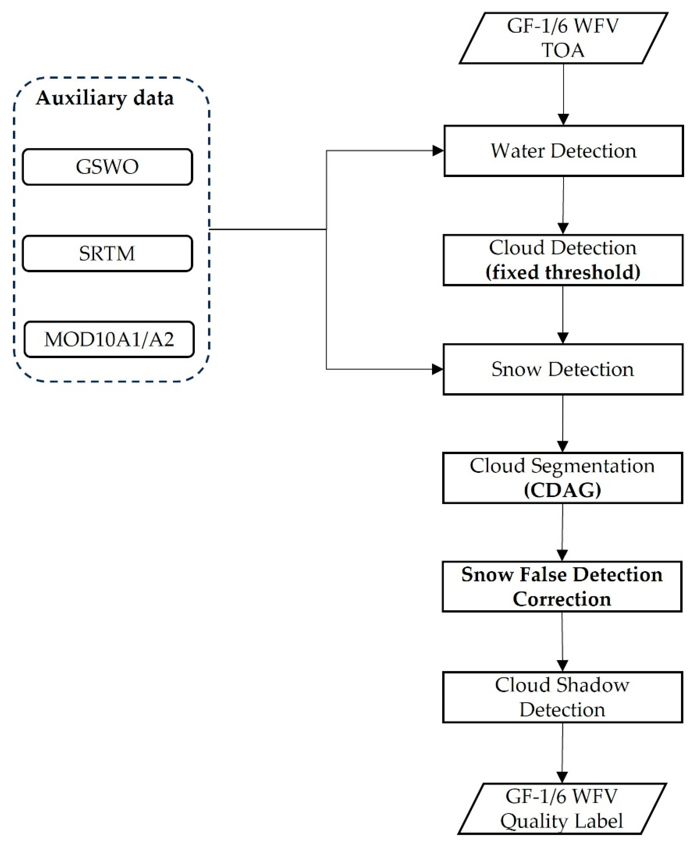
To meet the demand for producing the GF-1/6 WFV ARD quality marking data products, we should produce data products with similar accuracy to the Landsat series satellites and Sentinel-2 satellites. It should contain six categories: clouds, cloud shadows, snow, water bodies, land, and fill values. Figure 1 illustrates the GF-1/6 WFV ARD quality label algorithm’s processing flowchart.
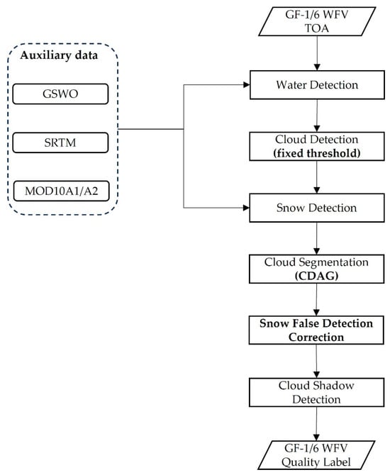
Figure 1.
GF-1/6 WFV ARD Quality Labeling Technological Flowchart.
The GF-1/6 WFV ARD quality tagging algorithm takes the Top of Atmosphere Reflectance (TOA) data as its input. Firstly, water body detection is performed using a threshold method along with auxiliary information from the Shuttle Radar Topography Mission (SRTM) and Global Surface Water Occurrence (GSWO) data. The SRTM data sets can be obtained from “https://earthexplorer.usgs.gov/ (accessed on 16 December 2022)” the source is: the United States Geological Survey (USGS). The GSWO dataset is available at “https://global-surface-water.appspot.com (accessed on 8 January 2023)” from EC JRC/Google. Then the coarse cloud detection based on a fixed threshold was performed, and the edge of the cloud region was corrected using guided filtering. The MODIS standard snow cover products MOD10A1/A2 determined whether snow exists in the current processing image. If there was no snow, we refined using guided filtering to get the final quality marker result. Our cloud detection used the Cloud Detection Algorithm Generator (CDAG) with automatic thresholds to correct cloud region results in the presence of snow while performing snow detection. Finally, the snow line is calculated using MOD10A1/A2 and SRTM data. It is utilized to simulate the presence of snow on mountains and correct any misdetections of snow-covered mountains within the cloud detection results.
2.2. Water Detection
The water detection process categorizes all pixels into two classes: water pixels and land pixels. One effective indicator for identifying water bodies is the near-infrared reflectance. This is because water exhibits a low reflectance in the near-infrared spectrum, whereas land typically has a relatively higher reflectance. In images, this contrast is manifested with water appearing dark and land appearing bright. The water detection process utilizes GSWO and SRTM data as auxiliary sources to refine the results based on a traditional thresholding method.
Moreover, the Normalized Difference Vegetation Index (NDVI) values play a crucial role in distinguishing between water and land pixels, as land areas typically exhibit higher NDVI values compared to water areas. Using the MFC algorithm [18], we have established thresholding rules to extract clear and turbid water bodies. The testing criteria are as follows:
The fixed-threshold method proved to be unreliable in accurately detecting water bodies, often misclassifying dark surfaces, cloud shadows, and mountainous terrain shadows as water bodies. To address this limitation, we employed GSWO data in combination with SRTM data for the correction of falsely detected water bodies. In order to account for geometric registration errors, for each connected region of water pixels, we check whether there are any water pixels marked by GSWO data within a 100-m radius. In cases where no matching pixel was found, the SRTM data was utilized to calculate the average elevation and slope of the linked area for the water body. If the average elevation exceeded the average water level in the region and a noticeable slope was present, we considered the water-connected area to be misdetected and corrected it to be considered a land surface. The average water level in the region was determined using statistical information from the GSWO and SRTM data. Our water detection algorithm utilized pre-downloaded GSWO and SRTM data, which were stored on the hard disk. The algorithm processed the GSWO and SRTM data to perform range selection, cropping, and reprojection based on the input image, resampling the spatial resolution to 16 m.
2.3. Fixed-Threshold Cloud Detection
The cloud detection in our algorithm mainly utilizes the fixed-threshold method. It is based on the premise that under clear-sky conditions the visible spectrum response of most land surfaces is highly correlated, whereas the spectral responses in the blue and red bands differ for haze and thin clouds. This approach significantly enhances our ability to differentiate between thin clouds and clear-sky conditions, contributing to the accuracy of our cloud detection process. The fixed-threshold cloud detection leverages the HOT index (Haze Optimized Transformation) [19], in conjunction with the Visible Band Ratio (VBR) index. The HOT index is constructed empirically based on the DN (Digital Number) values of clear-sky pixels, making it especially effective in distinguishing haze and thin clouds from clear-sky pixels. The calculation formulas for these indices are presented as follows:
Nevertheless, the fixed-threshold method is prone to generating numerous isolated points or discontinuities along the edges. Therefore, we employ guided filtering to enhance the precision of edge detection. Guided filtering was a simple and effective edge refinement algorithm [20]. The MFC algorithm employed guided filtering to process GF-1 WFV data to improve edge detection accuracy [11]. Most existing implementations of the guided filtering algorithm used the whole image as the matrix input. The computing time and memory consumption increased significantly as the image size increased. The MFC utilized a downsample to reduce the number of operations required for large-size GF-1 WFV image processing, which resulted in significant edge jaggedness. We aimed to optimize the guided filtering algorithm process to improve the efficiency of guided filtering for GF-1/6 large-size images. The blue band, which was significantly affected by atmospheric scattering, was noted as the guide map L (x, y), the cloud mask was noted as V (x, y), and the output image was noted as D (x, y). The calculation steps of the guided filtering algorithm were as follows:
- Step 1:
- Step 2:
- Step 3:
- Step 4:
- Step 5:
- Step 6:
In Steps 1 through 6, the application process of guided filtering in this paper is described. Step 1 involves computing the mean values, meanL and meanV, of the input image L and the guidance image V. In Step 2, the mean values, corrL (for the convolution of L and itself) and corrLV (for the convolution of L and V), are calculated. Steps 1 and 2 calculate the mean and variance of each pixel in the guidance image. These statistical measures are utilized for weighted averaging, enabling the consideration of the structure and characteristics of the guidance image during the smoothing of the target image. Step 3 employs covariance properties to compute the variances, varL (for L) and varLV (for the covariance of L and V). Covariance represents the degree of association between the guidance image and the target image. The computation of covariance is instrumental in determining weights that either enhance or diminish the influence of pixels during the smoothing process. In Step 4, weight ‘a’ is computed, and bias term ‘b’ is determined. In Step 4, using the mean and covariance information from the previous two steps, weights for each pixel are computed. These weights determine the relative contribution of pixel values from the guidance and target images considered during the smoothing operation. Step 5 calculates the averages, meana and meanb, of ‘a’ and ‘b’, respectively. Finally, in Step 6, the output image D (x, y) is obtained through the weighted addition of meana and meanb with the input image L, as per the formula. Steps 5 and 6 employ the calculated weights to conduct filtering operations on the target image. During the filtering process, more significant pixels are assigned greater weights, preserving image details while smoothing according to the structure of the guidance image.
The timely release of temporary matrix memory during the guided filtering calculation can reduce memory usage. For GF-6 large-size stitched WFV images, the temporary matrix was stored in the hard disk file to reduce memory usage. The extensive use of the median filter (fmean) in the computation of the guided filter was a significant factor affecting the computation time. To adapt to the transition region between large, thick clouds and surface areas, a filter radius of up to 100 pixels is adopted, significantly enhancing the computational efficiency of the median filter. The radius-independent Boxfilter fast median filtering algorithm reduced the computational complexity to approximately O (1) [21]. The Boxfilter first created a blank image with the same width and height as the original. Then, we assigned a pixel value to the sum of all pixels in the rectangle formed by that point and the image’s upper left corner. After the assignment, we used the pixels’ values at the four corners to calculate the sum of the pixels in a rectangle. Finally, we updated the value of each pixel to be the sum of pixels in the neighborhood. We can now directly access the corresponding position in the array whenever asking for the sum of pixels in a rectangle. We can obtain the corrected cloud areas from the output image D (x, y) > 0.14 based on guided filtering.
The quality labeled mask images sometimes had many areas with fewer than four connected pixel counts. For example, the highlighted ground surface in built-up areas was often frequently misclassified as clouds. Using the filtering function to filter out these discrete fragments and holes can effectively improve the mask quality and significantly reduce the number of pixel-linked regions. It also reduced the complexity of subsequent morphological processing operations with pixel-linked regions. This morphological correction process can eliminate false detections like highlighted surfaces and roads. For example, the MFC utilized the fractal dimension index (FRAC) and the length-to-width ratio (LWR) to filter false detections [11]. Morphological corrections were necessary for most of the data, but considering the complexity of clouds in real scenarios, the morphological correction step can be skipped selectively. Image processing algorithms such as the guided filtering, fragmentation filtering, and morphological methods cannot distinguish clouds from snow or some highlighted surface. However, they helped to improve cloud detection results, especially for transition boundaries.
2.4. Snow Detection
Snow detection aimed to determine whether the current image had a large area of snow cover in it. Snow detection identified the type of snow cover, such as snowy mountains, perennial snow, and seasonal snowfall, which helped with later snow identification and labeling.
Snow detection was performed using MODIS series satellites with 500-m resolution and the standard snow cover products MOD10A1 and MOD10A2. MOD10A1 was generated based on multi-band sensor images carried by Terra satellites and captured at 10:30 local time. We used satellite reflectance in bands 4 (0.545–0.565 μm) and 6 (1.628–1.652 μm) to calculate the Normalized Difference Snow Index (NDSI) for automatic snow cover mapping. The NDSI was calculated as follows:
NDSI is a calculation based on remote sensing bands, typically utilizing visible and near-infrared wavelengths. Snow exhibits higher reflectance in the visible spectrum and lower reflectance in the near-infrared spectrum, while other land cover types generally display the opposite characteristics. The computation of NDSI emphasizes this contrast between snow and non-snow, making snow more discernible. Additionally, because the reflectance properties of clouds in the visible and near-infrared bands typically differ from those of snow, NDSI aids in distinguishing between these two entities. We needed to adjust the NDSI threshold setting, and the NDSI > 0.4 threshold did not apply to all regions. For example, in the Tibetan Plateau, the optimal threshold is 0.1 [22,23]. According to the subsequent processing results, we can adjust the parameters. Combined with the threshold test rules and MODIS cloud mask data, some studies have shown an accuracy of about 94% for the binary daily scale snow product [24]. In this paper, we carried out snow detection using MOD10A1’s Fractional Snow Cover (FSC) band [25], where pixel values 0–100 indicated the ratio of snow cover and included water (239, 237), clouds (250), and fill-value (255) markers. The MOD10A2 was an 8-day synthetic data product obtained by further integration and processing [26]. It used the motion characteristics of the cloud to filter out the thickest cloud coverage and had higher accuracy. In accordance with prior research, the algorithm employed in MODIS standard snow products incorporates a “thermal mask” to enhance snow measurement outcomes. This inclusion effectively eliminates a significant portion of false snow detections, substantially reducing errors. The error rates of 8-day composite global maps have consistently remained low. For instance, in Australia, the error range across three sets of 8-day composite snow maps falls between 0.02% and 0.10% [27]. Hence, the utilization of MODIS standard snow products as our auxiliary data source for detection ensures a level of accuracy that is deemed sufficient.
The MOD10A1/A2 data was acquired through online automatic download to satisfy engineering applications. We can download MOD10A1/A2 data using the HTTPS request interface provided by the US Snow and Ice Data Center (NSIDC) “https://nsidc.org/data/MOD10A1 (accessed on 12 January 2023)” in HDF format. The MOD10A1 product can guarantee that for the input multispectral data imaging date, it can query the corresponding daily product data of the same day or one day before or after. Depending on the geographic coverage area of the input GF-1/6 multispectral image, over one scene of MOD10A1 product data may be retrieved. In that case, we utilized the command line to invoke the MODIS Reprojection Tool (MRT) batch interface to achieve the automatic stitching of the retrieved MOD10A1 data while selecting the snow cover data (FSC) band for conversion from HDF to TIFF format. This processing step generates a single-band snow cover image of byte type, with the same pixel size and map projection as the input GF-1/6 image. The snow cover image not only indicates snow pixels but also marks the categories of surface, water, cloud, and filling value. Due to the 500 m resolution of the image and the usage of nearest neighbor resampling to achieve 16 m resolution, a “tile” phenomenon may be observed in the output resulting from resampling.
The snow cover categories’ definitions were essential, influencing subsequent detection and correction techniques. This paper divided snow cover categories into snow mountains, perennial snow, and seasonal snowfall. Our category differentiation method counted the pixels of snow cover images with SRTM elevation. If the snow cover area is primarily mountainous, it is classified as snow mountains. In the absence of snow mountains, we calculate the snow image corresponding to the MOD10A1 and MOD10A2, excluding water and cloud regions. Then we judged whether the overlap proportion of snow cover contained in the surface snow cover was over 80%. If yes, it is a perennial snow area. Otherwise, it is a seasonal snowfall area. In the case of snowy mountains with perennial snow, subsequent processing will use the snow cover map produced by the MOD10A2 with fewer clouds. In case of seasonal snowfall with higher temporal sensitivity to snow cover changes, subsequent processing will use the snow cover map produced by the MOD10A1.
2.5. CDAG Cloud Segmentation
The results of the fixed-threshold cloud detection method included the incorrect identification of snow, as well as the utilization of consistent markers for pixel-linked regions. However, it was frequently observed that a pixel-linked region would contain both clouds and snow, which negatively impacted the accuracy of snow detection results that relied on the analysis of pixel-linked regions. To address this issue, the CDAG cloud detection algorithm aimed to further segment the effects of fixed-threshold cloud detection into distinct pixel-linked regions. This approach allowed for the categorization of different types of clouds in pixel-linked regions, taking into account the subtle spectral variations between clouds and snow across different bands. Such categorization provided the basis for subsequent corrections of snow misdetections.
The CDAG is a method for automatically generating cloud detection thresholds based on hyperspectral remote sensing data, of which accuracy has been verified on various sensors such as the MODIS, VIIRS, and Landsat8 OLI. Dong developed an improved CDAG algorithm for GF-6 WFV data cloud detection [8]. The CDAG is supported by a pre-determined hyperspectral database of cloud and clear sky pixels to simulate different types of multispectral sensor data. Then, it determines a suitable threshold based on the feedback of cloud detection accuracy generated by different bands and combinations of bands in the simulated data. When compared with cloud detection with fixed thresholds, the use of the combined thresholds of the CDAG on the scale of image elements can classify different cloud types.
The first step of the CDAG cloud detection algorithm involves the creation of a hyper-spectral dataset. This dataset consists of accurately labeled image elements representing different cloud types (thick clouds, thin clouds, broken clouds) as well as clear-sky image elements depicting various surface features such as cities, forests, water bodies, and bare ground. The cloud image elements are distributed across different surface backgrounds. The constructed hyperspectral dataset aims to simulate the image elements that would be captured by different multispectral sensors. To achieve this simulation, the CDAG algorithm utilizes the data simulation method proposed by He et al. [28]. This method establishes a relationship between hyperspectral and multispectral data based on the spectral response function of the sensor being simulated. Specifically, the broad-band data is obtained by simulating narrow-band data using specific equations and the spectral response function. The specific equations of the simulation are as follows:
where i denotes the i-band of the multispectral data, j denotes the j-band of the hyperspectral data, NH is the number of bands of the hyperspectral data, NM is the number of rounds of the multispectral data, RH j denotes the apparent reflectance of the image element of the hyperspectral data, denotes the evident reflectance of the image element of the multispectral data, Wj denotes the bandwidth of the hyperspectral data, and ρ(λi) represents the spectral response function of the hyperspectral data at wavelength λi. Finally, based on the simulated cloud and clear-sky image element database of the multispectral sensor, the correct cloud image element recognition rate and clear-sky image element recognition misclassification rate of different wavebands and waveband combinations at different thresholds are calculated. The threshold value for cloud detection is determined within the set allowable error range [9].
The CDAG faced challenges in effectively distinguishing between clouds and snow, often misidentifying snow as clouds in neighboring regions. In order to improve the segmentation of clouds and snow, CDAG focused its detection area solely on the cloud region within the cloud mask generated by the fixed-threshold cloud detection method. Specifically, for snowy mountain regions, the CDAG detected clouds within the intersection of the cloud mask region and the snowy mountain region. For perennial snow or seasonal snowfall regions, CDAG detected clouds within the intersection of the cloud mask region and the land region. However, the segmentation results of the CDAG sometimes contained fragmented areas and holes. To mitigate this, a filter was applied to retain only the pixel-linked regions with pixel counts greater than 1000. Despite these improvements, the CDAG still encountered challenges in cases where the spectra of clouds and snow were similar, but with distinct boundaries in adjacent transition regions. To address this issue, the SLIC algorithm can be employed as an alternative method to enhance the segmentation of adjacent cloud and snow regions using superpixel blocks [10].
2.6. Snow False Detection Correction
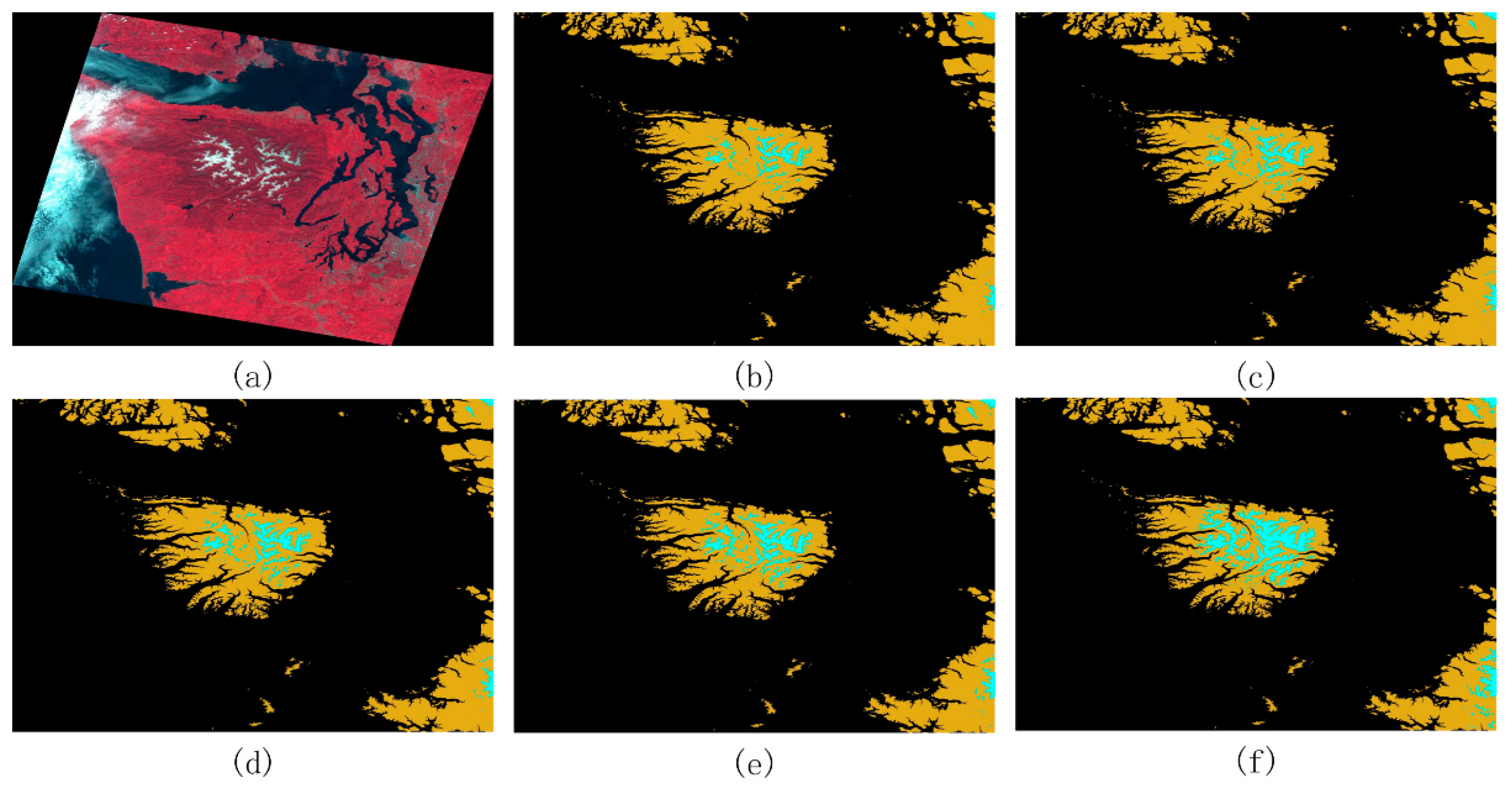
Snow false detection correction aimed to extract snow linkage regions from the cloud segmentation results where snow cover may be present. The snow misdetection correction algorithm differed according to the type of snow cover (mountainous areas, perennial snow, seasonal snowfall). The snow mountain simulation map served as the reference data for correcting snow mountain area misdetection, and the adopted method was region pixel matching. Figure 2 shows an example. The specific steps were: for each pixel association region in the snow mountain area, we generated a simulated snow mountain image S based on its outer wrapping rectangle of the geographical region R and the extracted snow line value with SRTM elevation; we counted the percentage of matching pixels between clouds pixels in region R and snow pixels in S, and also counted the percentage of matching pixels between surface pixels in region R and S. Considering the error between the simulated snow line and the actual height, five sequences of simulated snow mountain map , were generated using different values around the snow line elevation, then the pixel occupancy and of the sequences were obtained, , when there exists with and , and then the pixel-linked region was marked as snow. Otherwise, the original cloud marker was retained because there existed a situation where clouds were obscured a snowy mountain.

Figure 2.
Snow mountain area misdetection correction. [Yellow: the land surface; Cyan: snow] (b–f) depict the simulated snow coverage under varying snowline heights. The snowline progressively decreases from B to E, with a decrement of 50 m at each step, showcasing the corresponding outcomes. (a) GF-1 WFV TOA (RGB:432); (b–f) 5 snow mountain simulated maps with different snow line elevation values; (b) 1643 m; (c) 1593 m; (d) 1543 m; (e) 1493 m; (f) 1443 m.
The reference data for snow false detection correction in other snow cover areas (perennial snow, seasonal snowfall) was the snow cover map produced by MOD10A1/A2. This snow cover reference map had a raw resolution of only 500 m, which was also affected by clouds and may lack some places as well. So, the matching method for snowy mountain areas cannot be used. The processing step utilized here is cloud detection for the snow mountain area of pixels’ unicom area, statistics, and figure moderate snow matching pixel of the snow. Then if a snow pixel had no matching shadow area in its pixel-linked region in the subsequent cloud shadow detection step, the pixel-linked region was marked as snow. Otherwise, we kept the original cloud marker because there are cases where clouds obscure snow.
2.7. Cloud Shadow Detection
Cloud shadow detection was an essential part of the GF-1/6 quality labeling task, which consisted of two steps: shadow detection, and clouds and shadow matching. The shadow detection step mainly referred to the method of MFC [11]. The calculation formula is as follows:
The floodfill morphological transformation was applied to extract the local potential shadow areas. There were many dark surface areas in addition to cloud shadows in the detected shadow areas. The shadow and cloud matching step mainly referred to the method of Fmask. The fundamental concept behind the cloud-to-shadow matching method is to predict the position of cloud shadows by leveraging knowledge of the satellite sensor’s viewing angle, solar zenith angle, solar azimuth angle, and the relative altitude of the clouds. Given that the first three factors are known, they can be used to calculate the projection direction of cloud shadows. Along this direction, we employ the idea of cloud objects resembling the shape of their potential shadows and match cloud objects with potential shadow layers (Figure 3). The original cloud objects are excluded from the calculated shadows because a pixel cannot simultaneously belong to both cloud and shadow. The matching similarity for each cloud object is determined as the ratio of the overlapping area between the computed shadow and the potential cloud or shadow layer to the computed shadow area. To ensure the correct matching of cloud shadows, iterations are conducted on cloud height if the similarity increases or does not decrease to less than 98% of the maximum similarity; otherwise, the iteration is halted. If the similarity surpasses a specified threshold, the cloud shadow is considered a match; otherwise, it is rejected.
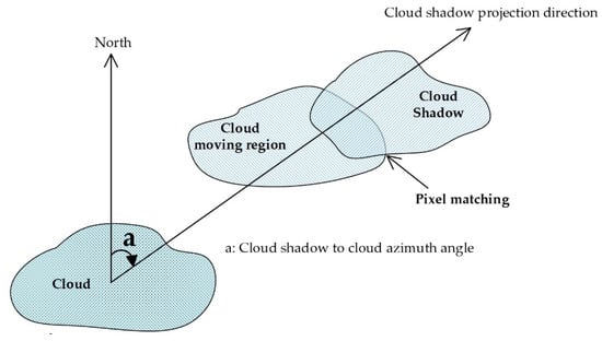
Figure 3.
The clouds and cloud shadow matches.
Unlike the existing methods, here when the processing image contains snow detection, shadow detection simultaneously counted the association area in the surface cloud area that did not match the shadows. If the percentage of snow pixels also existed, we corrected the pixel association area from clouds to snow. Cloud shadow masks were processed using the same image processing algorithms used for cloud detection—guided filtering, fragmentation filtering, and morphological filtering—to enhance the final cloud shadow mask’s quality. Figure 3 shows clouds and cloud shadow matches.
3. Experiments
This study aimed to achieve the effective segmentation of clouds and snow using GF-1/6 data quality tagging algorithms. The segmentation categories considered in this research encompassed clouds, cloud shadows, snow, water bodies, land, and fill values. In our efforts to enhance and optimize existing algorithms, we employed the fixed-threshold method for detecting clouds and cloud shadows based on the MFC approach [11]. Additionally, we utilized GSWO (Global Surface Water Occurrence) and SRTM (Shuttle Radar Topography Mission) data to segment water bodies and land regions, respectively. To validate the accuracy of our cloud–snow segmentation, we conducted experiments involving snowy mountain areas and snowfall scenarios, which served as the focal point of our research.
3.1. Experimental Data
Our test areas are situated along the west coast of the United States, in Washington State. This state is geographically divided by the Cascade Mountains, which separate the western region characterized by ample rainfall, and the majestic Mount Olympus overlooking temperate rainforests. The eastern part of the state, on the other hand, is dominated by the Columbia Lava Plateau, the Rocky Mountains, and vast desert areas, with the coastal climate influenced by the Pacific Ocean [29]. Washington State is further divided into seven distinct geographical regions, including the Olympic Peninsula in the northwest, housing the towering Olympic Mountains that reach a height of 2424 m, as well as the scenic Willapa Hills along the southern coast. In the northeast lies the Okanogan Highlands, ranging from 1200 to 2400 m above sea level. The complexity of Washington State’s climate, diverse surface types, and dramatic variations in snowlines on its mountainous terrain throughout the seasons make it an ideal location for the comprehensive testing of all quality marker categories. Notably, it is one of the nine selected global test areas for the Chinese satellite ARD project.
We used GF-1/6 WFV data with 16 m spatial resolution for our experiments. One hundred scenes imaged between January 2015 and December 2021 were selected, and 75 scenes containing snow mountains, with cloud coverage ranging from 10% to 80%. The data were raw Digital Number (DN) values, which we converted to TOA using calibration factors from the China Resources Satellite Application Center website (https://data.cresda.cn (accessed on 16 December 2022)). For the algorithm, we downloaded MODIS MOD10A1/A2 reference data online and processed them per view. We found that MOD10A2 data for the US region were relatively more complete. Figure 4 shows the distribution of the test areas and experimental data.
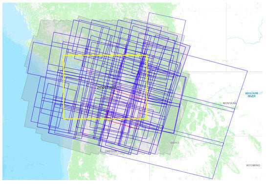
Figure 4.
Distribution of study areas and GF-1/6 data in Washington State, USA.
3.2. Algorithm Flow Experiments
Our GF-1/6 quality labeling algorithm comprised multiple steps utilizing various algorithms. The results of the critical steps directly affected the quality of the final marked products. In this chapter, we focused on analyzing the results of the newly added processing steps in the algorithm. We did not verify or analyze the GF-1/6 radiation calibration accuracy and threshold detection results here because published articles have already covered these topics.
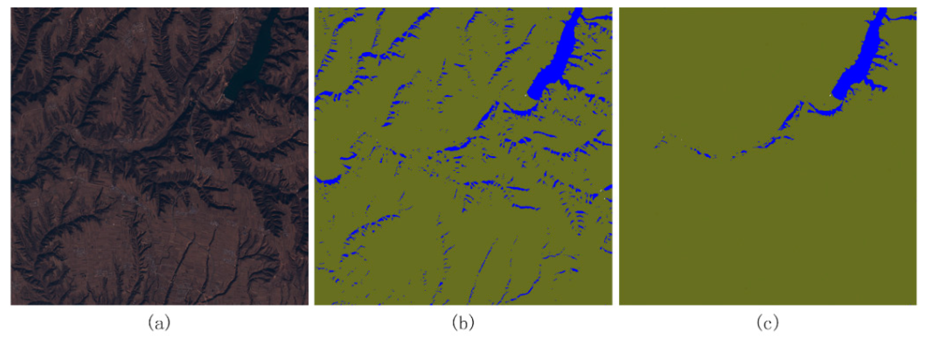
The fixed-threshold method in the water body detection step resulted in many false detections, including mountainous terrain shadows, cloud shadows, and other dark surfaces misidentified as water bodies. To correct these misdetected water bodies, we used GSWO with SRTM data, but we simplified the correction algorithm substantially. We manually verified the results of our experiments to ensure their effectiveness, as shown in Figure 5. This figure presents an example of a mountainous area where shadows were erroneously identified as water bodies, along with the corresponding corrective measures.
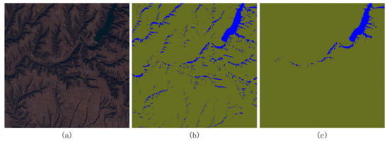
Figure 5.
Presents an example of the algorithm’s water body correction [Green: the land surface; Blue: water bodies]: (a) Partial GF-1 image with a pixel size of 512 × 512. (b) Conceptual diagram illustrating the outcomes of water detection using thresholding, which erroneously identifies some mountainous areas as water bodies. (c) Conceptual diagram showcasing the corrected results achieved by incorporating GSWO and SRTM data, effectively eliminating the misidentified mountainous regions.
While unable to distinguish clouds from snow and highlighted surfaces, image processing algorithms such as guided filtering, fragmentation filtering, and morphological methods can improve cloud detection results, particularly at transition boundaries. Figure 6 shows the correction example. The Figure 6a image contains thin clouds, thick clouds, and highlighted ground surface. The thresholding method used for detecting the region of the thin cloud in Figure 6b resulted in a regional omission. However, the guided map produced by guided filtering in Figure 6c effectively enhanced the influence range of the thin cloud region. The guided filtering resulting in Figure 6d corrected the boundary between thin and thick clouds, but there were still many discrete points and holes in the image. The fragmentation filtering algorithm in Figure 6e improved the quality of the cloud mask by reducing the number of pixel-linked regions and the number of morphological method operations. Finally, in Figure 6f, the morphological processing algorithm filtered out part of the highlighted surface dominated by built-up areas. These image processing algorithms also had a similarly significant effect in improving the mask quality in the cloud shadows detection step.
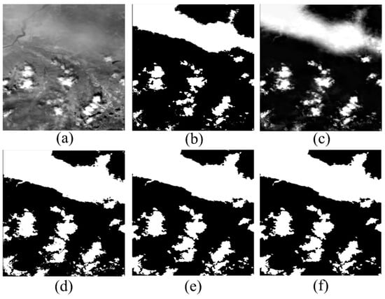
Figure 6.
Showcases an example of fixed-threshold cloud detection results and the subsequent correction using an image processing method [White: clouds; Black: the land surface]: (a) Original image depicting scenes with thin clouds, thick clouds, and bright surface areas. (b) Result of cloud detection using a fixed threshold, specifically highlighting the region with thin clouds. (c) Guided image used as input for guided filtering. (d) Result obtained after applying guided filtering. (e) Image after undergoing fragment filtering. (f) Image after further refinement through morphological processing.
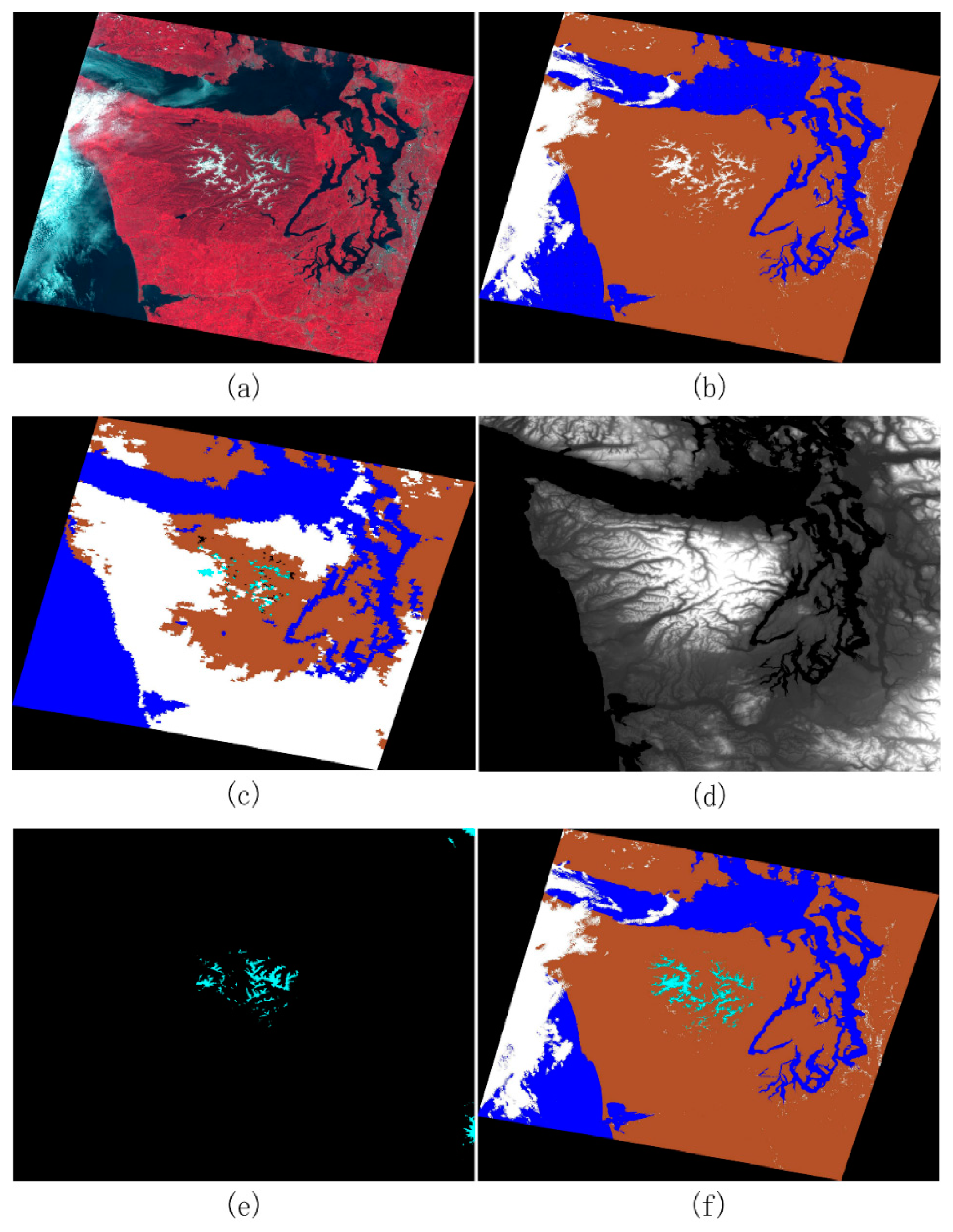
In this paper, we utilized MOD10A1/A2 data to verify the cloud detection result and determine if there was any snow misdetection. We used MOD10A1/A2 data for cloud snow segmentation. Figure 7 illustrates an example of extracting the misdetected snow from the cloud mask. The figure shows a 16-m resolution image acquired by the GF-1 WFV2 sensor, with bands Red (band 4), Green (band 3), and Blue (band 2). The image was taken in July 2017 at the Olympic Peninsula, Washington, USA, which contains Mount Olympus, a snowy mountain. In Figure 7b, the cloud mask shows that the snowy mountains are mistakenly detected as clouds. Figure 7c displays the snow-covered reference map obtained from the FSC band of the MODIS MOD10A1 data taken on the same day. It is cropped and reprojected from the source image to match the input image pixel by pixel. Since the original resolution is 500 m, the mosaic phenomenon is apparent after conversion to 16 m by the nearest neighbor sampling method. Meanwhile, the snow-covered reference map has cloud contamination (white areas) and low-quality areas (black areas). In Figure 7d, the SRTM elevation data is displayed, converted to the same size and resolution as the input image, with a 16 m resolution from 90 m bilinear interpolation. Figure 7e shows the snow mountain simulation image generated by calculating the base snow line using the snow cover reference map and the SRTM elevation map. According to the high-order simulation diagram, we generate a series of snow mountains near the snow line, which matches the following snow areas. Finally, Figure 7f shows the clouds–snow segmentation results with the snow cover type added to the cloud mask.
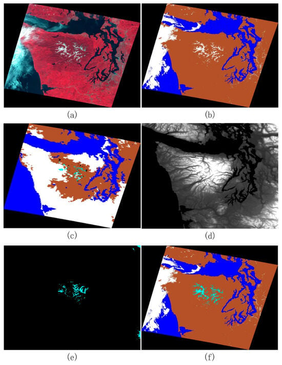
Figure 7.
GF-1/6 Quality Labeling Process Data Example (Olympic Peninsula, Mount Olympus). [Brown: the land surface; Blue: water bodies; Cyan: snow; White: clouds] (a) depicts the original image; (b) showcases the image where cloud detection errors occur; (c) displays MOD10A1 data with a spatial resolution of 500 m; (d) presents SRTM data with a spatial resolution of 90 m; (e) illustrates simulated snowy mountain conditions; (f) demonstrates the image after correcting the erroneously detected clouds as snow.
3.3. Results and Analysis
The Washington test area, located in the USA, features snow-covered mountains year-round, with the snowline experiencing substantial variations across seasons. Among the randomly selected sample of 100 images, 75 depict snowy mountains, while the majority of the remaining images are affected by cloud contamination. For the purpose of this paper, we focused on processing the 75 images that captured snow-capped mountains. We employed manual visual interpretation to assess the impact of the cloud–snow segmentation algorithm.
We divided the 75 images depicting snowy mountains into two groups based on the distribution and adjacency of clouds and snow. Group A comprised images that were either cloud-free or contained clouds that had minimal adjacency with the snow. This group consisted of a total of 23 images. On the other hand, Group B included images where clouds covered either the entirety or a portion of the snowy mountains. Within Group B, there were a total of 52 scenes.
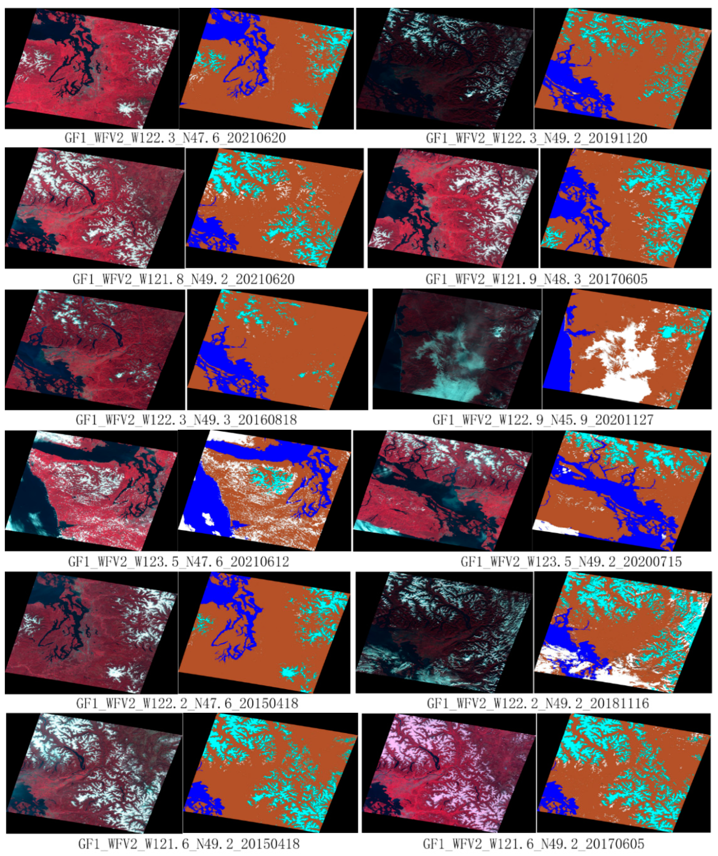
Figure 8 shows a partial example of the processing results for Group A. Our algorithm can effectively segment the clouds and snow in most snow mountain areas. Since the pixel-linked areas of clouds were not adjacent to snow mountains, there was no case of cloud areas being mistakenly corrected for snow. Therefore, the cloud–snow segmentation processing of Group A data improved the accuracy of the GF-1/6 satellite quality-labeled data products. Figure 9 shows a partial example of the processing results for Group B. Overall, snow was effectively identified, but there were cases where some regions with clouds were corrected to snow. Since a pixel-linked region contained clouds and snow categories, there was no valid segmentation boundary before the algorithm corrected the pixel-linked region where snow was present to snow. The algorithm counted whether the pixel contained a certain percentage of surface neighbors outside the edge of the linked region within the mountainous terrain area. If the linked region was surrounded by all cloud pixels, the snowy mountain was considered to be entirely covered by clouds, and the linked area remained cloudy with any pixel marker. However, if clouds did not entirely cover the pixel linkage area, the linkage area was relabeled as snow. While snow was detected under this correction strategy, it mostly led to some cloud regions being mislabeled as snow.

Figure 8.
Examples of cloud–snow segmentation for group A data (clouds and snow regions separated) [Brown: the land surface; Blue: water bodies; Cyan: snow; White: clouds]. These images serve as examples of cloud–snow segmentation, where the cloud and snow regions are mostly distinct. The depicted scenes either lack clouds entirely or exhibit minimal adjacency between the clouds and snow-covered areas.
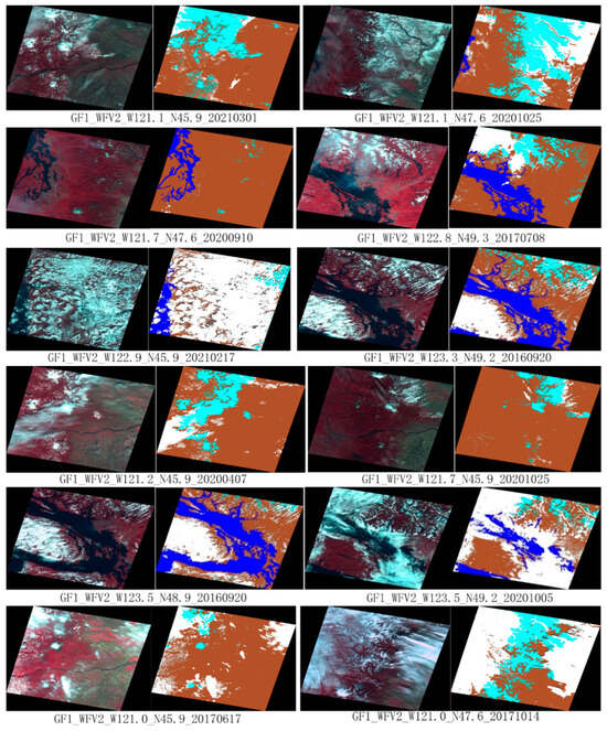
Figure 9.
Examples of cloud–snow segmentation for group B data (clouds and snow regions adjacent) [Brown: the land surface; Blue: water bodies; Cyan: snow; White: clouds]. This collection of images presents illustrative examples of cloud–snow segmentation, demonstrating scenarios where the cloud regions exhibit significant adjacency to the snow-covered areas. In these images, clouds are present and cover either the entire snow-capped mountains or a substantial portion thereof.
The processing results were classified into three ratings, namely, good, improved, and bad, to evaluate the overall impact of cloud–snow segmentation on enhancing the quality of labeled data products. The good rating indicated that the corrected snow mountain was accurate, with no cloud–snow mixing errors. The improved rating indicated that the corrected snow mountain was predominantly precise, although some cloud–snow mixing errors were present. However, the area of misclassified correction was smaller than that of correctly classified correction. On the other hand, the bad rating indicated that the corrected snow mountain was predominantly accurate. However, there were cloud–snow mixing errors, and the area of incorrect correction exceeded that of correct correction.
We used direct manual visual interpretation to grade the results. It was difficult to distinguish the boundary between clouds and snow and to quantitatively calculate the area ratio between the incorrect and correct corrections. Manual visual interpretation allowed for the easy and quick determination of the area comparison between the correct and incorrect corrections. If the correct and incorrect corrections area was similar in manual visual interpretation, it was classified as bad, although the ratio was similar in very few cases. Table 2. presents the results of 75 image classifications using the three-level rating method. The ratio of good to improved was more than 70% (23 + 30)/75 × 100%). For data adjacent to the cloud–snow region, the number of improvements exceeded the number of bad ratings. Even for data with bad ratings, it is clear from Figure 9 that the areas where cloud areas are misclassified as snow correspond to surfaces with a high probability of being snow.

Table 2.
Cloud–Snow Segmentation Result Ratings.
3.4. Accuracy Evaluation
To assess the performance of our method, this research utilizes overall accuracy as the evaluation metric [9]. By comparing the cloud detection results with visually inspected judgments, we determine the overall accuracy of our approach. Given the substantial effort required for visual inspection, a randomly selected region of 300 × 300 pixels within the images is used for visual judgments and compared against the cloud detection results. The formula for calculating overall accuracy is as follows:
where TP denotes the count of correctly detected cloud pixels, TN refers to the accurate identification of non-cloud pixels, and N represents the total number of pixels in the image.
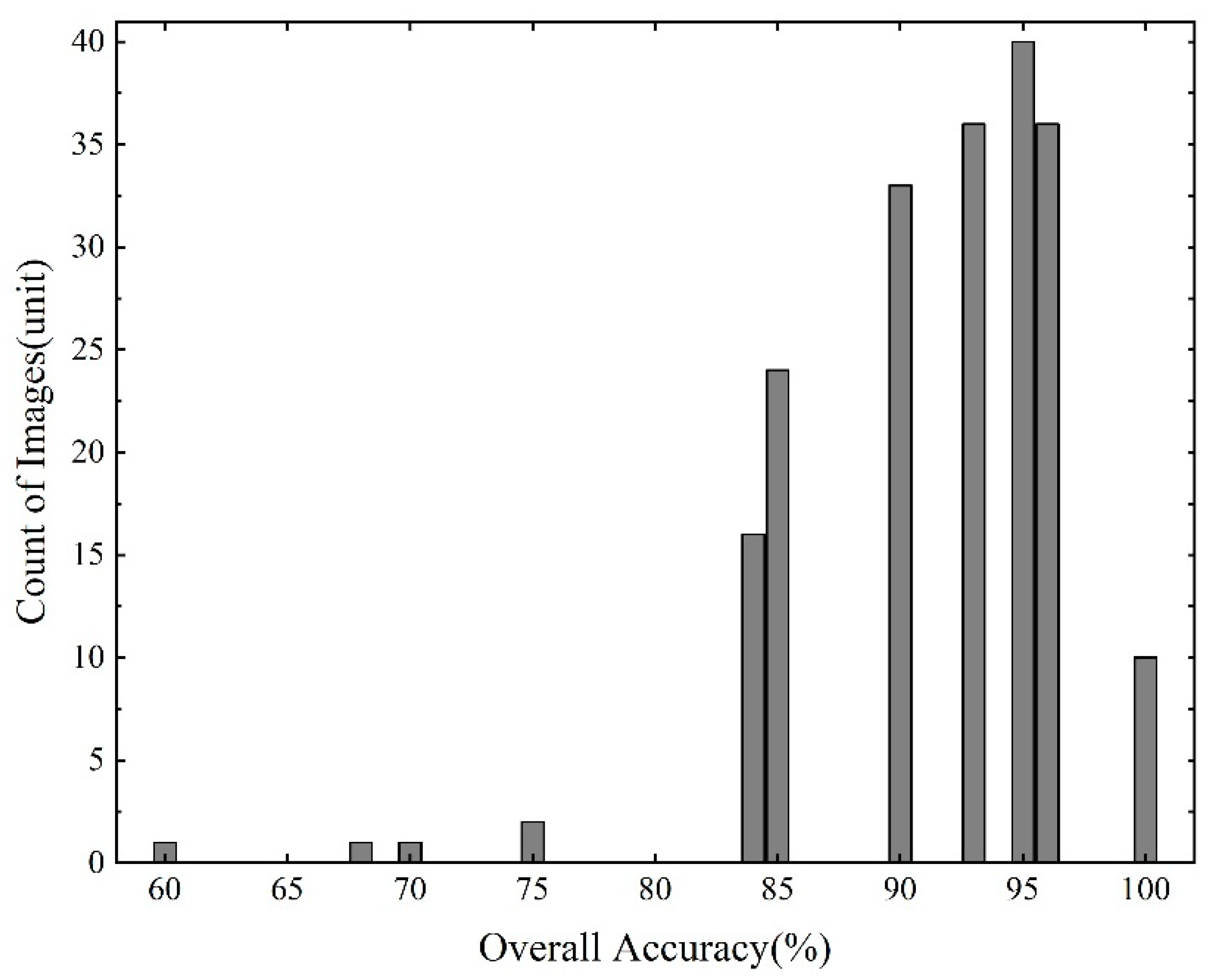
The overall accuracy, as depicted in Figure 10, was calculated based on 200 randomly selected regions (300 × 300 pixels) from a pool of 75 images, resulting in an average overall accuracy of 91.53%. The graph illustrates that over 77% of the tested images exhibit a high degree of overall accuracy. However, the utilization of low-resolution MODIS data and subsequent resampling do impact the overall accuracy of cloud detection, resulting in a slight decline. Furthermore, there are instances where certain test images yielded an overall accuracy below 80%. A detailed examination of these images revealed that the MOD10A2 data still encompasses a substantial proportion of snow-covered areas obstructed by clouds, thereby compromising the precision of snow mountain simulation. Nonetheless, several images achieved an overall accuracy surpassing 90%, underscoring the robust performance of our algorithm in effectively discerning between clouds and snow.
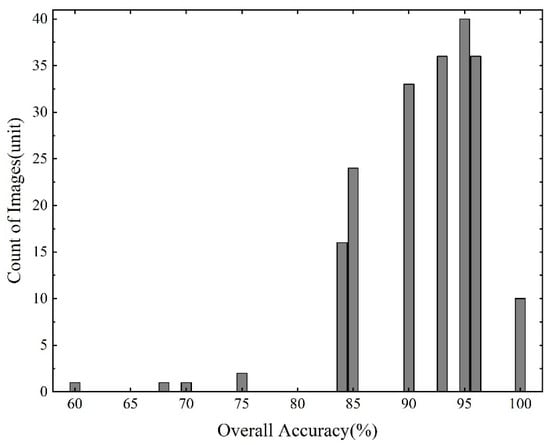
Figure 10.
Illustrates a statistical graph depicting the overall accuracy of the algorithm.
4. Discussion
The Chinese GF-1/6 satellites possess exceptional spatial resolution, enabling detailed observations of surface features. However, cloud cover can greatly impede accurate observations of these features. Given the challenge of distinguishing between clouds and snow using thresholding methods alone, this study introduces a new approach to alleviate cloud detection errors in snow-covered mountain areas by utilizing MODIS standard snow products. Experimental results show that the proposed method achieves a high level of precision in detecting clouds and cloud shadows. Furthermore, successful differentiation between clouds and snow is effectively achieved within the designated study area.
However, some errors persist in the cloud detection results. Firstly, our reliance on MODIS standard snow products, which are closely aligned with the imaging dates of the GF-1/6 satellite multispectral images, introduces challenges. Not all GF-1/6 satellite data scenes have readily available and corresponding MODIS standard snow products from similar timeframes. This limitation may potentially hinder the effectiveness of our algorithm for a small subset of GF-1/6 satellite images. Secondly, the MODIS standard snow products we utilized have a spatial resolution of 500 m. To match the 16 m spatial resolution of our experiments, we resampled these products, resulting in “tiling” effects that could impact subsequent snow detection. In future work, we aim to investigate techniques for improving snow detection. Additionally, cloud contamination remains a significant factor that affects the accuracy of our algorithm. The MOD10A2 data may still include a substantial proportion of snow-covered areas obscured by clouds, compromising the precision of snow mountain simulation. Furthermore, with regards to GF-1/6 images, our method may incorrectly identify cloud and cloud shadow regions above the snow-covered areas as either snow or land. Therefore, the detection of cloud shadows represents an important area of focus for our future research efforts.
5. Conclusions
This study introduced a methodology for rectifying snow detection errors in cloud detection using MODIS standard snow products as reference data. By incorporating guided filtering, fragment filtering, morphological filtering, and other algorithms into the existing fixed-threshold cloud detection, we successfully addressed the challenge of snow misclassifications in cloud detection for the Chinese GF-1/6 satellite. Our approach substantially enhances the precision of cloud detection and establishes a comprehensive GF-1/6 satellite quality marking algorithm encompassing six categories: cloud, cloud shadow, snow, water body, land, and fill value. These advancements effectively meet the requirements of the “Chinese Satellite ARD” project.
The conclusions drawn from these experimental results are as follows: (1) The proposed method demonstrates excellent performance. The experiments utilized six years of data from Washington State, USA. By comprehensively comparing manually interpreted scenes and statistical analysis, an accurate discrimination rate of over 70% for snow-covered scenes was achieved, with an overall average accuracy of cloud detection reaching 91%. (2) The integration of MODIS standard snow products data with GSWO\SRTM data enables effective differentiation between clouds and snow, thereby rectifying instances where snow is mistakenly classified as clouds.
The primary contributions of this work are as follows: (1) We proposed a novel approach to address the issue of snow misclassifications in cloud detection for the Chinese GF-1/6 satellite. By utilizing MODIS standard snow products, we rectify these misclassifications during cloud detection. (2) Our method offers a unique solution to the challenges faced by the Chinese GF-1/6 multispectral satellite, which lacks shortwave infrared and thermal infrared bands. These limitations make it difficult to distinguish between clouds and snow. (3) The proposed method allows for the generation of cloud masks and other quality marking data. These data can be utilized for subsequent engineering applications of ARD. Furthermore, while deep learning methods have shown effectiveness, their limitations often arise from the scarcity of high-quality training datasets. However, by leveraging the processed results obtained from our algorithm and conducting meticulous manual accuracy inspections, we can create substantial quantities of quality-marked training samples. Therefore, one of our future research directions involves investigating deep learning approaches for quality marking algorithms. Overall, these contributions provide valuable insights into improving cloud detection and snow discrimination for the Chinese GF-1/6 satellite. This advancement enables the application of satellite data in various fields.
Author Contributions
Conceptualization, H.C. and C.H.; methodology, H.C. and C.H.; software, C.H.; validation, X.F.; data curation, H.C. and X.F.; writing—original draft, H.C. and X.F.; writing—review and editing, C.H. and L.H.; visualization, H.C.; supervision, C.H. and L.H. All authors have read and agreed to the published version of the manuscript.
Funding
This work is partly supported by the National Key Research and Development Program of China (grant number 2019YFE0197800) and the National Natural Science Foundation of China (grant number 41971396).
Conflicts of Interest
The authors declare no conflict of interest.
References
- Zou, Z.; Chen, K.; Shi, Z.; Guo, Y.; Ye, J. Object Detection in 20 Years: A Survey. Proc. IEEE 2023, 111, 257–276. [Google Scholar] [CrossRef]
- Zou, Z.; Shi, Z. Ship Detection in Spaceborne Optical Image with SVD Networks. IEEE Trans. Geosci. Remote Sens. 2016, 54, 5832–5845. [Google Scholar] [CrossRef]
- Ma, A.; Wang, J.; Zhong, Y.; Zheng, Z. FactSeg: Foreground Activation-Driven Small Object Semantic Segmentation in Large-Scale Remote Sensing Imagery. IEEE Trans. Geosci. Remote Sens. 2021, 60, 5606216. [Google Scholar] [CrossRef]
- Chen, H.; Li, W.; Shi, Z. Adversarial Instance Augmentation for Building Change Detection in Remote Sensing Images. IEEE Trans. Geosci. Remote Sens. 2021, 60, 5603216. [Google Scholar] [CrossRef]
- King, M.D.; Platnick, S.; Menzel, W.P.; Ackerman, S.A.; Hubanks, P.A. Spatial and Temporal Distribution of Clouds Observed by MODIS Onboard the Terra and Aqua Satellites. IEEE Trans. Geosci. Remote Sens. 2013, 51, 3826–3852. [Google Scholar] [CrossRef]
- Irish, R.R.; Barker, J.L.; Goward, S.N.; Arvidson, T. Characterization of the Landsat-7 ETM+ automated cloud-cover assessment (ACCA) algorithm. Photogramm. Eng. Remote Sens. 2006, 72, 1179–1188. [Google Scholar] [CrossRef]
- Zhu, Z.; Woodcock, C.E. Object-based cloud and cloud shadow detection in Landsat imagery. Remote Sens. Environ. 2012, 118, 83–94. [Google Scholar] [CrossRef]
- Dong, Z.; Sun, L.; Liu, X.; Wang, Y.; Liang, T. CDAG-Improved Algorithm and Its Application to GF-6 WFV Data Cloud Detection. Acta Opt. Sin. 2020, 40, 1628001. [Google Scholar] [CrossRef]
- Sun, L.; Mi, X.; Wei, J.; Wang, J.; Tian, X.; Yu, H.; Gan, P. A cloud detection algorithm-generating method for remote sensing data at visible to short-wave infrared wavelengths. Isprs J. Photogramm. Remote Sens. 2017, 124, 70–88. [Google Scholar] [CrossRef]
- Wang, M.; Zhang, Z.; Dong, Z.; Jin, S.; Su, H. Stream-computing Based High Accuracy On-board Real-time Cloud Detection for High Resolution Optical Satellite Imagery. Acta Geod. Cartogr. Sin. 2018, 47, 760–769. [Google Scholar]
- Li, Z.; Shen, H.; Li, H.; Xia, G.; Gamba, P.; Zhang, L. Multi-feature combined cloud and cloud shadow detection in GaoFen-1 wide field of view imagery. Remote Sens. Environ. 2017, 191, 342–358. [Google Scholar] [CrossRef]
- Hu, C.; Zhang, Z.; Tang, P. Research on multispectral satellite image cloud and cloud shadow detection algorithm of domestic satellite. J. Remote Sens. 2023, 27, 623–634. [Google Scholar] [CrossRef]
- Liu, Z.; Wu, Y. A review of cloud detection methods in remote sensing images. Remote Sens. Land Resour. 2017, 29, 6–12. [Google Scholar]
- Shao, Z.; Pan, Y.; Diao, C.; Cai, J. Cloud Detection in Remote Sensing Images Based on Multiscale Features-Convolutional Neural Network. IEEE Trans. Geosci. Remote Sens. 2019, 57, 4062–4076. [Google Scholar] [CrossRef]
- Jiao, L.; Huo, L.-Z.; Hu, C.; Tang, P. Refined UNet v3: Efficient end-to-end patch-wise network for cloud and shadow segmentation with multi-channel spectral features. Neural Netw. 2021, 143, 767–782. [Google Scholar] [CrossRef] [PubMed]
- Li, Z.; Shen, H.; Cheng, Q.; Liu, Y.; You, S.; He, Z. Deep learning based cloud detection for medium and high resolution remote sensing images of different sensors. Isprs J. Photogramm. Remote Sens. 2019, 150, 197–212. [Google Scholar] [CrossRef]
- Yan, Z.; Yan, M.; Sun, H.; Fu, K.; Hong, J.; Sun, J.; Zhang, Y.; Sun, X. Cloud and Cloud Shadow Detection Using Multilevel Feature Fused Segmentation Network. IEEE Geosci. Remote Sens. Lett. 2018, 15, 1600–1604. [Google Scholar] [CrossRef]
- Yu, J.; Li, Y.; Zheng, X.; Zhong, Y.; He, P. An Effective Cloud Detection Method for Gaofen-5 Images via Deep Learning. Remote Sens. 2020, 12, 2106. [Google Scholar] [CrossRef]
- Zhang, Y.; Guindon, B.; Cihlar, J. An image transform to characterize and compensate for spatial variations in thin cloud contamination of Landsat images. Remote Sens. Environ. 2002, 82, 173–187. [Google Scholar] [CrossRef]
- He, K.; Sun, J.; Tang, X. Guided Image Filtering. IEEE Trans. Pattern Anal. Mach. Intell. 2013, 35, 1397–1409. [Google Scholar] [CrossRef]
- Viola, P.; Jones, M. Rapid object detection using a boosted cascade of simple features. In Proceedings of the Conference on Computer Vision and Pattern Recognition, Kauai, HI, USA, 8–14 December 2001. [Google Scholar]
- Tang, Z.; Wang, J.; Li, H.; Liang, J.; Li, C.; Wang, X. Extraction and assessment of snowline altitude over the Tibetan plateau using MODIS fractional snow cover data (2001 to 2013). J. Appl. Remote Sens. 2014, 8, 084689. [Google Scholar] [CrossRef]
- Zhang, Y.; Cao, T.; Kan, X.; Wang, J.; Tian, W. Spatial and Temporal Variation Analysis of Snow Cover Using MODIS over Qinghai-Tibetan Plateau during 2003–2014. J. Indian Soc. Remote Sens. 2017, 45, 887–897. [Google Scholar] [CrossRef]
- Hall, D.K.; Riggs, G.A. Accuracy assessment of the MODIS snow products. Hydrol. Process. 2007, 21, 1534–1547. [Google Scholar] [CrossRef]
- Salomonson, V.V.; Appel, I. Estimating fractional snow cover from MODIS using the normalized difference snow index. Remote Sens. Environ. 2004, 89, 351–360. [Google Scholar] [CrossRef]
- Wang, X.; Xie, H.; Liang, T. Evaluation of MODIS snow cover and cloud mask and its application in Northern Xinjiang, China. Remote Sens. Environ. 2008, 112, 1497–1513. [Google Scholar] [CrossRef]
- Hall, D.K.; Riggs, G.A.; Salomonson, V.V.; DiGirolamo, N.E.; Bayr, K.J. MODIS snow-cover products. Remote Sens. Environ. Interdiscip. J. 2002, 83, 181–194. [Google Scholar] [CrossRef]
- He, L.; Qin, Q.M.; Meng, Q.Y.; Du, C. Simulation of Remote Sensing Images Using High-Resolution Data and Spectral Libraries. In Proceedings of the 4th International Conference on Environmental Science and Information Application Technology (ESIAT 2012), Bali, Indonesia, 1–2 December 2012. [Google Scholar]
- Fosu, B.O.; Wang, S.Y.S.; Yoon, J.H. The 2014/15 snowpack drought in washington state and its climate forcing. Bull. Am. Meteorol. Soc. 2016, 97, S19–S24. [Google Scholar] [CrossRef]
Disclaimer/Publisher’s Note: The statements, opinions and data contained in all publications are solely those of the individual author(s) and contributor(s) and not of MDPI and/or the editor(s). MDPI and/or the editor(s) disclaim responsibility for any injury to people or property resulting from any ideas, methods, instructions or products referred to in the content. |
© 2023 by the authors. Licensee MDPI, Basel, Switzerland. This article is an open access article distributed under the terms and conditions of the Creative Commons Attribution (CC BY) license (https://creativecommons.org/licenses/by/4.0/).

