Article

Improving 3D Digital Soil Mapping Based on Spatialized Lab Soil Spectral Information

1
State Key Laboratory of Soil and Sustainable Agriculture, Institute of Soil Science, Chinese Academy of Sciences, Nanjing 210008, China
2
College of Forestry, Henan Agricultural University, Zhengzhou 450002, China
3
University of Chinese Academy of Sciences, Beijing 100049, China
4
Key Laboratory of Watershed Geographic Science, Nanjing Institute of Geography and Limnology, Chinese Academy of Sciences, Nanjing 210008, China
*
Author to whom correspondence should be addressed.
Remote Sens. 2023, 15(21), 5228; https://doi.org/10.3390/rs15215228
Submission received: 19 September 2023 / Revised: 17 October 2023 / Accepted: 18 October 2023 / Published: 3 November 2023
(This article belongs to the Section Remote Sensing in Agriculture and Vegetation)

Abstract

:
Readily available environmental covariates in current digital soil mapping usually do not indicate the spatial differences between deep soil attributes. This, to a large extent, leads to a decrease in the accuracy of 3D soil mapping with depth, which seriously affects the quality of soil information generated. This study tested the hypothesis that spatialized laboratory soil spectral information can be used as environmental covariates to improve the accuracy of 3D soil attribute mapping and proposed a new type of environmental covariable. In the first step, with soil-forming environmental covariates and independent soil profiles, laboratory vis-NIR spectral data of soil samples resampled into six bands in Anhui province, China, were spatially interpolated to generate spatial distributions of soil spectral measurements at multiple depths. In the second step, we constructed three sets of covariates using the laboratory soil spectral distribution maps at multiple depths: conventional soil-forming variables (C), conventional soil-forming variables plus satellite remote sensing wavebands (C+SRS) and conventional soil-forming variables plus spatialized laboratory soil spectral information (C+LSS). In the third step, we used the three sets of environmental covariates to develop random forest models for predicting soil attributes (pH; CEC, cation exchange capacity; Silt; SOC, soil organic carbon; TP, total phosphorus) at multiple depths. We compared the 3D soil mapping accuracies between these three sets of covariates based on another dataset of 132 soil profiles (collected in the 1980s). The results show that the use of spatialized laboratory soil spectral information as additional environmental covariates has a 50% improvement in prediction accuracy compared with that of only conventional covariates, and a 30% improvement in prediction accuracy compared with that of the satellite remote sensing wavebands as additional covariates. This indicates that spatialized laboratory soil spectral information can improve the accuracy of 3D digital soil mapping.

1. Introduction

Environmental covariates are spatially continuous and have a synergistic relationship with soil spatial variability. They can be the variables characterizing factors such as the soil itself, climate, biology, topography, parent material, time and spatial location in the SCORPAN model [1].
Environmental covariates are key to digital soil mapping. Their ability to indicate soil spatial variability largely determines the upper limit of prediction accuracy and modeling complexity that can be achieved by soil mapping. The upper limit of soil prediction accuracy is higher when there are covariates with strong indication, which is high spatial synergy between soil attributes and environmental covariates. It is not necessary to have a complex model, and a simple model can achieve high accuracy. On the contrary, the upper limit is lower when there are covariates with weak indication, which is low spatial synergy between soil attributes and environmental covariates, and even complex models still achieve low accuracy.
Thus, in order to obtain the spatial distribution of prepared soil information, great emphasis has been put on the use of environmental covariates in digital soil mapping [1]. For example, Liu et al. [2,3] proposed a surface dynamic feedback approach to develop effective covariates to improve soil mapping in gentle topographic areas where easily accessible topographic and vegetation variables had weak synergistic relationships with soils. A review of 30 years of digital soil mapping showed that more than 70% of the works had used topography as covariates and more than 30% had used vegetation as covariates [4].
Improper selection of environmental covariates often does not adequately characterize soil-forming environmental conditions. Climate variables such as temperature and precipitation can be generated by spatial interpolation of weather station data. Topographic variables can be generated by digital terrain analysis of the DEM, and vegetation and land use variables are obtained by remote sensing observations. Many studies have shown that these existing covariates have a strong relationship with soil attributes at upper depths and a weak relationship with soil attributes at lower depths [5,6,7,8]. The soil parent materials have a strong relationship with the underlying soil. Chen et al. [4] argued that this was valid for soil organic carbon/soil organic matter, bulk density and particle size fractions (Clay, Silt, Sand), but not for pH and AWC. Meanwhile, it is difficult to obtain information on the spatial distribution of the parent materials through direct observation over a large area. Thus, the accuracy of 3D digital soil mapping of soil attributes usually decays with depth. This seriously affects the quality of soil information and adds great uncertainty to the simulations of hydrological, climate and soil pollution processes. Therefore, how to improve the accuracy of 3D digital soil mapping is an urgent research problem to be solved.
Developing new environmental covariates that can capture spatial differences in the subsoil is a direct solution. Heung et al. [9] developed a random forest model between parent material types and topographic variables for predictive mapping of the parent material types in a study area of British Columbia, Canada. Visible near-infrared (vis-NIR) remote sensing can only detect soil information at the depth of a few centimeters on the extreme surface in bare soil conditions. Geophysical remote sensing such as Gamma-ray spectroscopy can partially reflect the information of the parent material. Loiseau et al. [10] showed that airborne Gamma spectral remote sensing data were useful covariates for predictive mapping of surface soil texture in a plot in western France. However, the maximum detection depth of an airborne approach was 30 cm [11,12,13]. For sediments, Gamma spectra are mainly associated with the content of clay particles. For bedrock, Gamma spectral signals come from the minerals and are mainly applied to the detection of clay particle contents. Electromagnetic induction instruments can measure the electrical conductivity of soil particles. They are more sensitive to soil physicochemical attributes such as soil salinity, clay particle content, water content and nutrients. Møller et al. [14] used portable ground-based electromagnetic induction sensor measurements as covariates and performed high-resolution mapping of clay and organic matter content. However, for large-area applications, the consistency of measurement data is difficult to guarantee.
Laboratory soil spectra contain a wealth of information that can reflect a variety of soil attributes, including soil organic matter, total nitrogen, soil texture, conductivity [15], moisture content, iron oxide content, carbonate minerals and pollutant content [16,17]. Many regional and national soil spectral libraries have been established internationally [13,18] and global soil spectrum libraries [19] are under construction. They contain various spectral bands such as visible, near-infrared and mid-infrared. The spectral information was measured under controlled laboratory conditions for soil samples at different depths after air-drying and grinding treatment. They can reflect the physical and chemical information of underlying soil materials. However, laboratory soil spectra are mainly limited and discrete point data and cannot be used directly as environmental covariates to assist in the predictive mapping of soil attributes.
The purpose of this study is to propose a method for improving 3D digital soil mapping based on laboratory soil spectral information by testing the hypothesis that using spatialized laboratory soil spectral information can improve the accuracy of 3D soil mapping, that is, spatialized laboratory soil spectral information and its derived factors are developed and used as environmental covariates to assist in improving the prediction accuracy of 3D mapping.

2. Materials and Methods

2.1. Study Area

The study area is Anhui Province, China. Anhui Province lies between 114°54′–119°37′E and 29°41′–34°38′N, with a total area of 140,100 km2. According to the Soil Series of Anhui Province [20], it is in a transition between a warm temperate zone and a subtropical zone. It has a humid climate and obvious seasonal changes because of the influence of the southeast subtropical monsoon. The average annual temperature is 14–17 °C and the average annual precipitation is 773–1670 mm. Precipitation gradually decreases from southeast to northwest. The study area has various types of landforms, including plains, terraces, hills and mountains. The northern part is the Huaibei plain area and the main land use is dryland. The central part is the hilly area of the Jianghuai Terrace and the plain area along the river has low elevation. Its main land uses are drylands and paddy fields. The southern part is a hilly mountain area with high elevation and undulating terrain. The main land uses are forests, grasslands and paddy fields.
The soil types in the study area include Calcaric Cambisols, Cutanic Luvisols, Eutric Cambisols, Eutric Regosols, Ferralic Cambisols, Ferric Acrisols, Ferric Lucisols, Haplic Fluvisols, Hydragric Anhtrosols and Lithic Leptosols. They are determined based on the World Reference Base for Soil Resources [21]. Among them, Hydragric Anhtrosols, Hydragric Anhtrosols and Calcaric Cambisols are the most widely distributed.

2.2. Soil Attributes Data

We used 132 typical soil profiles in this study (Figure 1). They originated from the Second National Soil Survey in the 1980s and represent the typical soil landscape in the study area. Soil attributes were measured for each horizon of the soil profiles. They are soil pH, cation exchange capacity, organic carbon content, soil texture and total phosphorus content.
We used equal-area quadratic spline functions [22,23] to simulate the depth distribution of the five soil attributes and computed the values of soil attributes at five fixed depths: 0–5, 5–15, 15–30, 30–60 and 60–100 cm. Table 1 lists the statistical description of the soil attributes at these depths. As the depth increases, soil pH and Silt show an increasing trend, while cation exchange capacity, soil organic carbon and total phosphorus all have different degrees of decrease. The standard deviations (SDs) of all soil attributes except soil pH are high and the data dispersion is significant. The dispersion of soil attributes increases with increasing depth; this leads to a decrease in predictability. Among them, soil organic carbon and total phosphorus have coefficients of variation (CV) greater than 0.5. The spatial variations between different soil profiles are obvious.

2.3. Laboratory Soil Spectral Data

An additional set of soil profile data were used to determine laboratory soil spectral information in this study; these data were derived from the project National Soil Series Survey and Soil Series of China [3]. The survey period was from 2010 to 2011, with a total of 114 soil profiles. Soil horizon samples were subjected to a continuous drying process, fully ground and passed through a 2 mm sieve. The vis-NIR reflectance data of each soil sample were measured using a Cary 5000 spectrophotometer (Agilent Technologies, Santa Clara, CA, USA) under controlled temperature and humidity conditions in the laboratory [24]. We recorded ten soil spectral repeats in each soil sample. The measured spectral band range was 350–2500 nm, with a resolution of 1 nm.
Denoising and dimensionality reduction were performed for laboratory soil spectral data. In the first step, large fluctuating noises usually occur at the beginning and end of the measurement phase due to the influence of the external environment. The noisy 350–399 nm and 2401–2500 nm bands were artificially removed and the soil spectral data at 400–2400 nm were retained. In the second step, a small number of information-rich spectral bands, which are sensitive to most soil attributes, were selected [24]. These are red band (R, 620–680 nm), green band (G, 520–600 nm), blue band (B, 430–460 nm), NIR short-wave band (SW-NIR, 840–890 nm), NIR mid-wave band (MW-NIR, 1550–1750 nm) and NIR long-wave band (LW-NIR, 2100–2300 nm). We averaged the spectral reflectance data within each band to obtain the mean reflectance data of the six bands. In the fourth step, we used equal-area quadratic spline functions to normalize the mean values of the six laboratory soil spectral characteristic bands and generated reflectance values at the five fixed depths of 0–5 cm, 5–15 cm, 15–30 cm, 30–60 cm and 60–100 cm [25].

2.4. Environmental Covariates

Table 2 lists the environmental covariates used in this study. They were classified into parent material variables, topographic variables, climatic variables, biological variables and satellite remote sensing waveband variables. In this study, we collected the environmental covariates that changed over time (such as climatic variables and biological variables) in two different periods. One period (2010s) of the environmental covariates was used to make spatial prediction of the laboratory soil spectral information. The other period (1980s) of environmental covariates was used to verify the improvement in spatialized laboratory soil spectral information on the accuracy of 3D mapping of soil attributes. For environmental covariates that did not change over time, we collected data in only one period.
Parent material variables were 1:21 million Soil Parent Materials map of China, obtained from Geographic Data Sharing Infrastructure, College of Urban and Environmental Science, Peking University (http://geodata.pku.edu.cn, accessed on 7 October 2021). Topographic variables were obtained based on 90 m spatial resolution SRTM DEM data (http://srtm.csi.cgiar.org/srtmdata, accessed on 7 October 2021), calculated using SAGA GIS software (http://www.saga-gis.org, accessed on 7 October 2021). Climate variables from the 1980s were 1 km spatial resolution climate data from the WorldClim database. They were all annual averages from 1970 to 2000 [26]. The climate variables from the 2010s are derived from the 1 km resolution climate and precipitation dataset of China drawn by Peng et al. [27]. Biological variables from the 2010s were NDVI and EVI from the MODIS data product (MOD13Q1) and biological variables from the 1980s were obtained by time downscaling using climate variables from the 1980s. Satellite remote sensing waveband variables from the 2010s were MODIS reflectance data from 7 bands (MOD09A1). Both biological variables and satellite remote sensing variables were obtained through the GEE platform and their mean values were calculated from the average data for the years 2000–2010. All environmental covariates were unified into the Albers projection coordinates system and resampled to 1 km resolution.

2.5. Methods

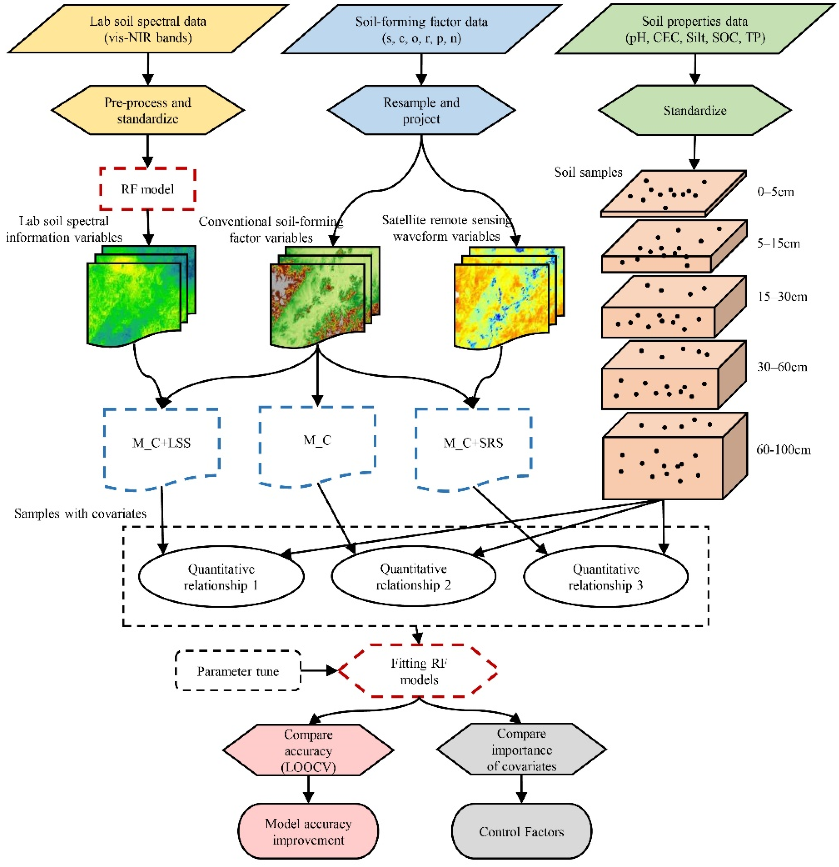
The method for testing the hypothesis consisted of three steps (Figure 2). In the first step, we spatialized the laboratory soil spectra to generate multiple-depth soil spectral-spatial distribution layers. In the second step, we constructed three sets of environmental covariates with the variables in Table 2 and the spatialized laboratory soil spectral variables. In the third step, we compared the three sets of covariates by assessing their 3D soil attribute mapping accuracies.

2.5.1. Spatialization of Laboratory Soil Spectra

We used a random forest model [28] to construct a quantitative relationship between laboratory soil spectral information and soil-forming environmental covariates (elev, anHis, slp, curPln, curPrf, TWI, TPI, MAT, tempSeason, tempWettest, windspeed, LST, NDVI, etc.). The random forest model is an integrated decision tree model that can reduce the overfitting of decision trees to a certain extent. It has the advantages of easy training and high accuracy and is currently a mainstream machine learning method [29,30,31]. This model randomly generates several decision trees for classification and regression problems. Each tree randomly draws data from training samples to include in the training process. The final prediction result is the average of the prediction results of all decision trees. Another advantage of the model is that the importance of input covariates can be judged by the out-of-bag mean square error values (%lncMSE) and the nodal bluntness values (lncNodePurity). Higher %lncMSE and lncNodePurity represent larger contributions of the covariate to the prediction results. We determined the optimal parameters of the model based on the out-of-bag prediction results and predicted spatial distributions of the laboratory soil spectral bands (R, G, B, SW-NIR, MW-NIR, LW-NIR) at 1 km spatial resolution at the 5 standard depths.
We selected four error metrics to calculate the accuracy of the spatialization of laboratory soil spectral information using the leave-one-out-cross validation (LOOCV) method [32]. These are mean error (ME), root mean square error (RMSE), coefficient of determination (R2) and Concordance Correlation Coefficient (CCC) [33], which were calculated as follows:
M E = 1 n i = 1 n O i P i
R M S E = 1 n i = 1 n O i P i 2
R 2 = 1 i = 1 n O i P i 2 i = 1 n O i O ¯ 2
C C C = 2 r σ O σ P σ O 2 + σ P 2 + O ¯ P ¯ 2
where O i and P i are the observed and predicted values of sample i; n is the total number of samples; O ¯ and P ¯ are the mean values of the sample observed values and predicted values; r is the correlation coefficient between the predicted and observed values of the samples; σ O and σ P are the standard deviations of the sample observation and predictions.
The construction of the random forest model is based on the open source R environment [34] and involves the packages “randomForest” [35], “caret” [36], “rgdal” [37], “raster” [38] and “ggplot2” [39].

2.5.2. Constructing Sets of Environmental Covariates

We constructed three sets of environmental covariates and compared their predictive performance for soil attributes. The first set is the conventional soil-forming variables (C), which includes terrain, climate and biological variables. The second set is the combination of conventional soil-forming variables and satellite remote sensing wavebands variables (C+SRS) with the purpose of checking the accuracy improvement in 3D soil attribute prediction when adding satellite remote sensing information in the covariates. The wavebands include short-wave NIR, blue and long-wave NIR. The third set is the combination of conventional soil-forming variables and laboratory soil spectral information variables (C+LSS) with the purpose of checking the accuracy improvement in 3D soil attribute prediction when adding laboratory soil spectral information to the covariates. We combined the 6 laboratory soil spectral bands to generate 12 soil spectral correlation factors, aiming to generate some laboratory soil spectral factor combinations by referring to the common combination of satellite remote sensing bands so as to expand the application range of soil spectral information. Table 3 lists the calculated expressions for the 12 soil spectral correlation factors.

2.5.3. Assessing Accuracy Improvements in 3D Soil Attribute Predictions

For each set of covariates and each of the soil attributes (pH, CEC, Silt, SOC, TP), we used a random forest model to construct their quantitative relationships at each depth. We trained all models with default parameters with the purpose of excluding the effect of different parameters on the model performance. We then used the LOOCV to assess the prediction accuracy of all models. The error metrics R2 and RMSE were calculated using Equations (2) and (3). Then, we calculated the relative accuracy improvements in R2 and RMSE of covariate sets C+SRS and C+LSS over covariate set C using the following equations [40].
R I R 2 = R M x 2 R M c 2 R M c 2
R I R M S E = R M S E M c R M S E M x R M S E M c
where R I R 2 and R I R M S E are the relative improvements, respectively, in R2 and RMSE; R M x 2 and R M S E M x are, respectively, the R2 and RMSE for covariate set C+SRS or C+LSS; R M c 2 and R M S E M c are, respectively, the R2 and RMSE for covariate set C. Higher R I R 2 or R I R M S E values mean a bigger accuracy improvement.

3. Results

3.1. Covariates of Laboratory Soil Spectra

Table 4 lists the accuracies of spatial predictions of laboratory soil spectral bands R, G, B, SW-NIR, MW-NIR and LW-NIR. It shows that the ME values are close to 0 and the CCC values are mainly distributed between 0.4 and 0.7. This indicates a good agreement between the predicted and observed values. The R2 values are mainly concentrated between 0.3 and 0.5, with an average of 0.36. This means the random forest algorithm is able to explain nearly 36% of the laboratory soil spectral information.
Figure 3 shows the spatialized laboratory soil spectral bands at five depth intervals. The laboratory soil spectral reflection values were relatively low in the northern plains and high in the southern hills. In the vertical dimension, the laboratory soil spectral reflection values showed an increasing trend with depth. In addition, the laboratory soil spectral reflectance showed an increasing trend with increasing wavelength. The lowest reflectance value was in the blue band. The highest reflectance value was in the mid-wave near-infrared band.

3.2. Correlations between Soil Attributes and Spatialized Laboratory Soil Spectral Information with Covariates

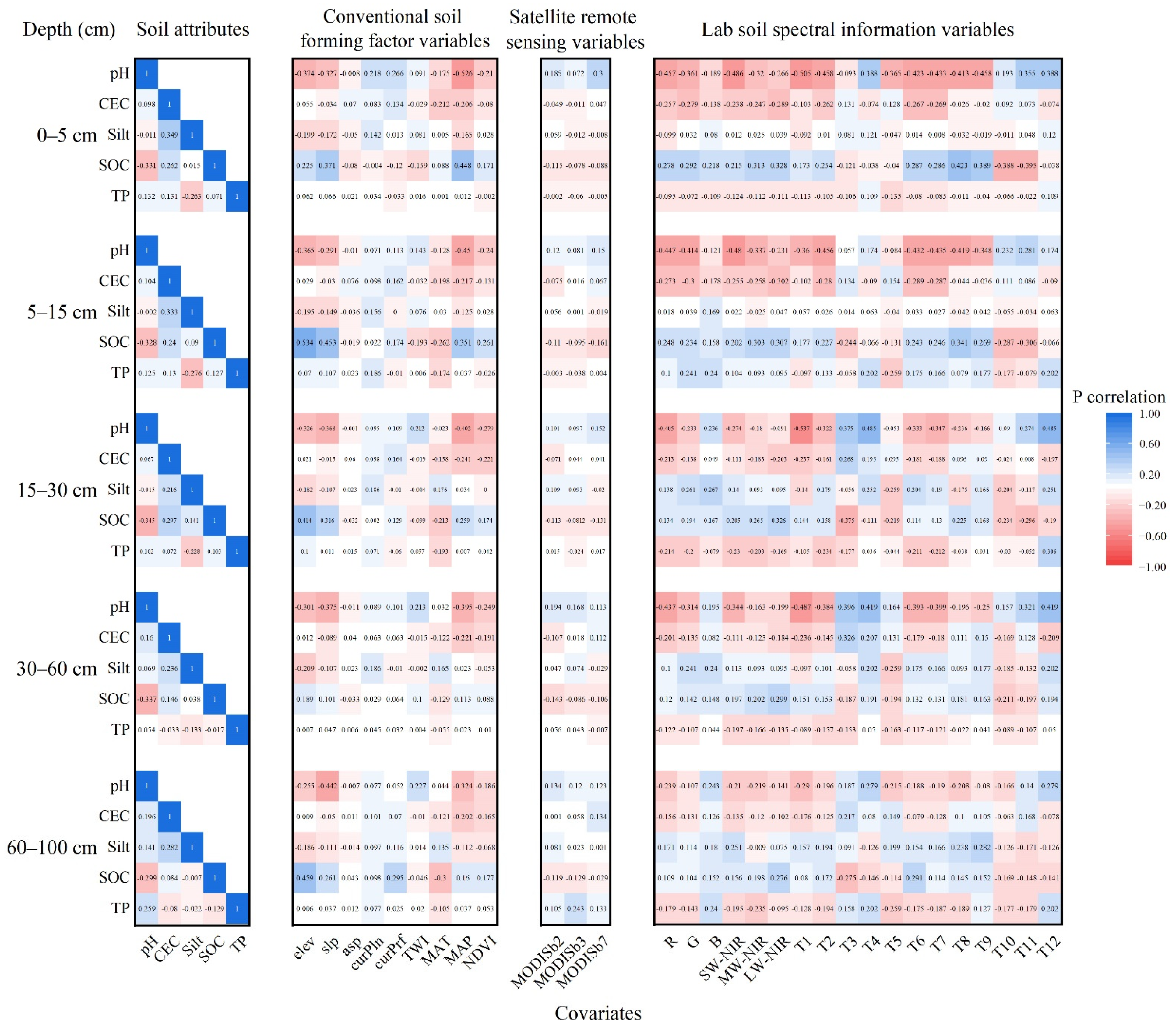
Figure 4 shows Pearson correlation matrices between soil attributes and environmental covariates at different depths. Overall, soil pH, CEC and SOC were strongly correlated with all covariates, while Silt and TP were weakly correlated with the covariates. The correlation between each soil attribute and covariate decreased with increasing depth.
Table 5 lists the significance tests of correlation coefficients between the soil attributes at different depths and satellite remote sensing waveband variables or laboratory soil spectral variables. It can be seen that the correlation coefficients of the soil attributes with laboratory soil spectral variables were significantly higher than those with satellite remote sensing waveband variables at different depths (p < 0.05). This indicates that laboratory soil spectral information had a higher correlation with soil attributes than satellite remote-sensing wavebands.

3.3. Performance Improvement of 3D Soil Attribute Mapping

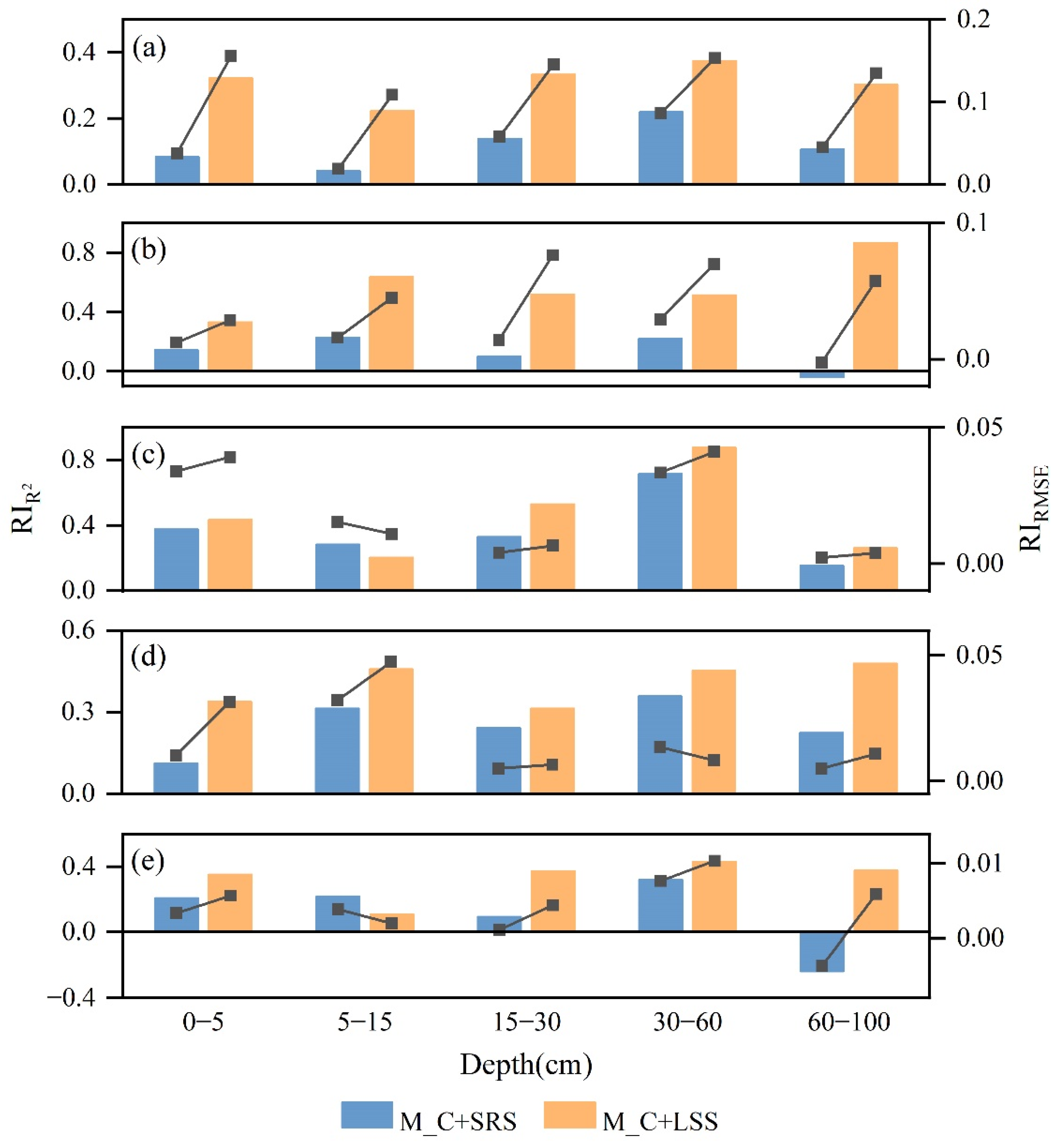
Figure 5 shows the improvement in 3D prediction accuracies of covariate set C+SRS and covariate set C+LSS over covariate set C. Covariate set C+LSS achieved 30~80% accuracy improvement (40% on average) compared with covariate set C; it achieved about 30% accuracy improvement compared with covariate set C+SRS. This indicates that the addition of laboratory soil spectral information can effectively improve the accuracy of 3D mapping of soil attributes relative to conventional soil-forming variables. Laboratory soil spectral information had a higher accuracy enhancement effect compared with satellite remote sensing information. Laboratory soil spectral information was obtained by direct spectral measurement of soil samples, which does not have the interference observed for other factors such as atmosphere, temperature and humidity. Thus, it is a more intuitive response to changes in soil attributes compared with conventional soil-forming and satellite remote-sensing variables.
The average R2 improvements for the C+LSS covariate set compared with the C covariate set were, respectively, 31.14%, 57.26%, 46.08%, 40.78% and 32.90% for soil pH, CEC, Silt, SOC and TP, while those for the C+SRS covariate set were, respectively, 11.75%, 14.51%, 37.19%, 24.93%, and 11.98%. This indicates that using laboratory soil spectral information as covariates can produce higher accuracy compared with satellite remote sensing information. Satellite remote sensing sensors are susceptible to the influence of ground cover when capturing reflectance information in the bare soil state during ground observation. Soil CEC, Silt and SOC have direct correlations with soil spectral information, and thus their prediction accuracy with the C+LSS covariate set is better than other attributes.
Table 6 lists the means of the accuracy improvements in the soil attributes at 0–60 cm and 60–100 cm depths when using the C+SRS and the C+LSS covariate sets. It shows that the accuracy improvements tend to decrease with increasing depth when using the C+SRS covariate set. Accuracy improvements for CEC, SOC and TP tend to increase with the increase in depth when using the C+LSS covariate set. This is because satellite remote sensing can only capture soil information on the surface layer, while laboratory soil spectral information is the result of direct observation of soil samples and is capable of observing soil samples at any depth. Its prediction accuracy depends only on the correspondence between soil attributes and soil spectral information and it can effectively improve the situation such that the prediction accuracy of soil attributes decreases with depth.
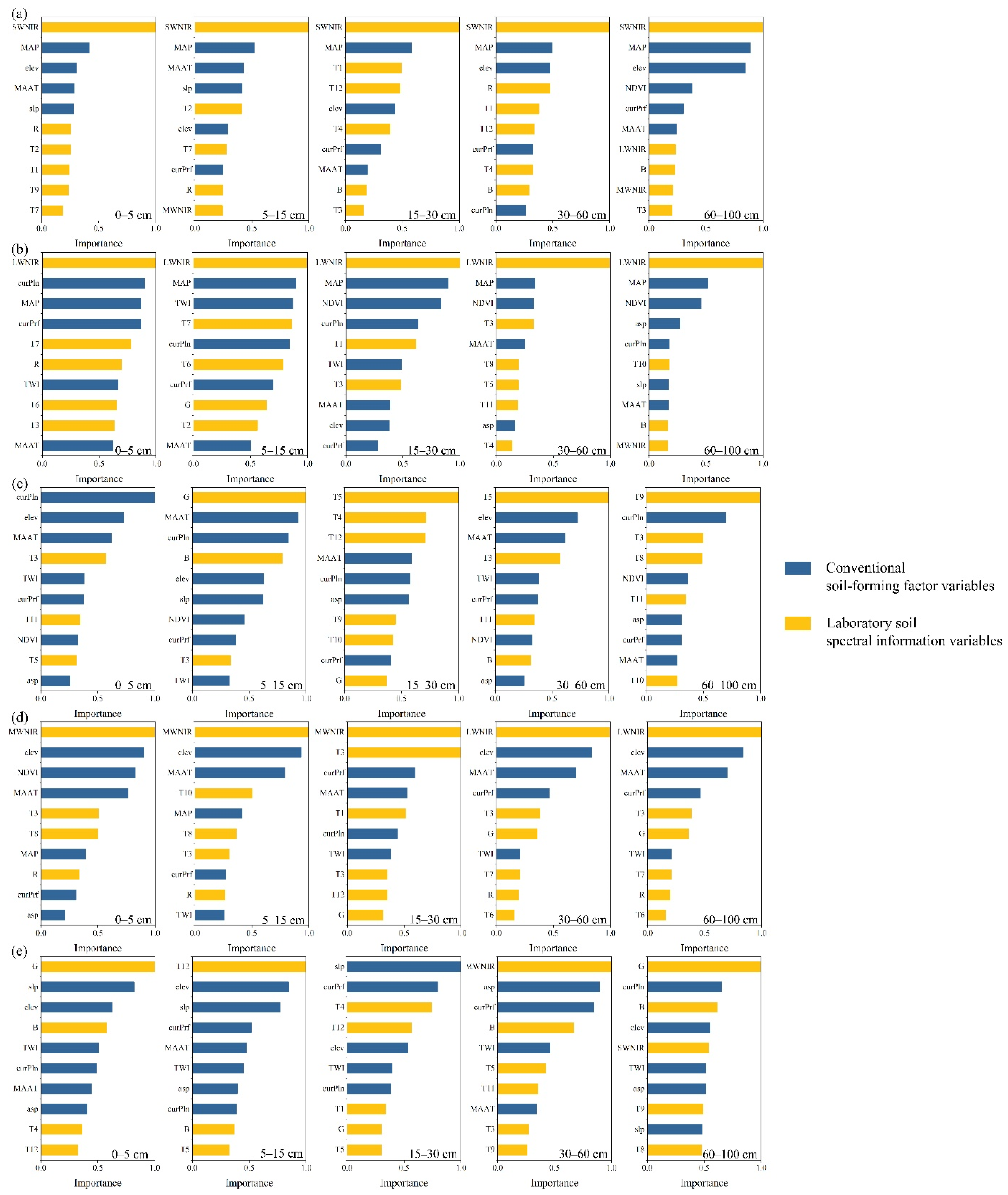
Figure 6 shows the relative importance of the top 10 C+LSS covariates. blue represents conventional soil-forming variables and yellow represents laboratory soil spectral variables. It can be seen that the laboratory soil spectral information played an important role in the prediction of the spatial distribution of all the soil attributes. SW-NIR and LW-NIR were, respectively, the most important covariates for soil pH and CEC. G, T5 and T9 were the most important covariates for Silt at depths below 5 cm, which mainly respond to the effect of NIR short-wave band and green wave band on soil texture. LW-NIR and MW-NIR were the most important covariates for SOC. The soil spectral information in the near-infrared band has a good inversion capability for soil organic carbon. G, MW-NIR and T12 were the most important covariates for TP in soils below 5 cm depth.
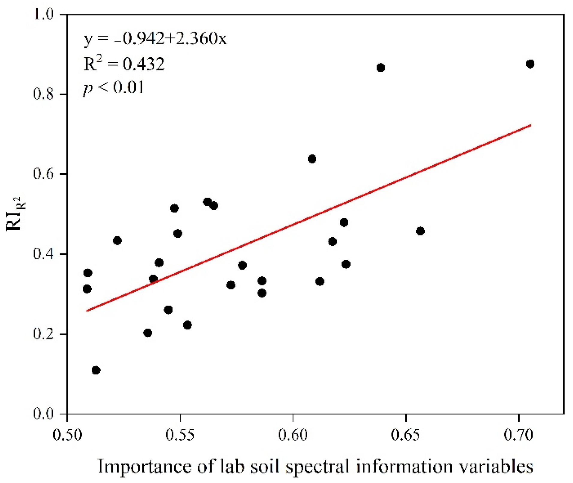
Figure 7 shows the relative importance percentage of conventional soil-forming variables and laboratory soil spectral variables in the C+LSS covariate set. It can be seen that the laboratory soil spectral variables were more important than the conventional soil-forming variables at different depths for all five soil attributes. Figure 8 shows the scatter plot of the relative importance percentage of laboratory soil spectral information against the prediction accuracy improvement in the C+LSS covariate set. They had an overall positive correlation (p < 0.01). The higher the relative importance of laboratory soil spectral variables, the bigger the accuracy improvement for different soil attributes and depths.

4. Discussion

4.1. Predictability of Laboratory Soil Spectral Information

Table 4 and Figure 3 show that the prediction of laboratory soil spectral information in different bands can be realized using spatial speculation. The constructed model can predict the spectral information of soil in the laboratory well and has a certain accuracy (Table 4). At the same time, the spectral information of laboratory soil predicted by the random forest model has obvious spatial distribution characteristics.
The prediction results of soil spectral information in the laboratory have obvious horizontal and vertical distribution characteristics. They were affected by the geographical landscape, topographic position and soil attributes. The central alluvial areas have small soil particle sizes that influence the absorption characteristics of soil and result in a reduction in soil spectral reflectance [41,42]. Since soil organic carbon decreases with increasing depth, the soil in the lower depth usually has high spectral reflection [43,44].
At the same time, we found a relatively high correlation between laboratory soil spectral information and general soil attributes (Figure 4). The correlation coefficients of soil pH, CEC and SOC with laboratory soil spectral bands were relatively high. This is because soil organic matter content can influence soil spectral information in the near-infrared band [45]. The negative charge carried on the surface of soil organic matter can regulate soil acid buffering and thus affect soil pH [46,47]. The correlations between Silt and TP with each covariate at the 0–15 cm depth were weak. Due to the high agricultural activities in the study area, tillage and fertilization interfered with the nutrient composition of the topsoil. This led to a decrease in the correlation between the texture and nutrient content of the topsoil and the covariates; intermediate and deeper soil Silt and TP had high correlations with the vis-NIR bands of laboratory soil spectra and some spectral correlation factors.

4.2. Advantages of Laboratory Soil Spectral Information as Covariates

First, vis-NIR remote sensing can identify surface vegetation information and detect soil information only at a depth of about 3–5 cm on the extreme surface of the soil under bare soil conditions [48]. However, it is susceptible to interference from factors such as atmosphere and surface moisture. Although microwave remote sensing can penetrate the atmosphere and detect a certain depth of soil, it is also affected by the roughness of the ground surface, moisture and other factors. The laboratory soil spectral information is a direct hyperspectral detection of air-dried and ground soil samples under controlled laboratory conditions. The obtained spectral information is more representative of the physical and chemical attributes of the soil itself [15]. The soil samples were collected through soil surveys and the observation depth depends on the depth of the soil profile excavation. Many studies show high accuracy of soil spectral inversion of multiple soil attributes [49,50,51]. Using laboratory soil spectral information as covariates significantly increased the ability to capture soil attributes at lower depths and complemented the defects that remote sensing covariates primarily capture surface environmental information.
Second, the vis-NIR bands of laboratory soil spectral information are spectroscopically associated with many soil attributes. They can effectively differentiate soil types and predict soil attributes such as soil organic matter, soil texture, moisture content, iron oxide content, carbonate minerals and contaminant content [52,53,54]. The absorption bands at 400–800 nm, 1700–1900 nm and 2100–2400 nm can characterize the soil organic matter content. The absorption bands at 1300–1500 nm and 1800–2500 nm are sensitive to mineral content. The LW-NIR band at 1800–2100 nm can respond to information associated with soil moisture content. The binding band at 400–1000 nm reflects the distribution of iron oxides in the soil. The absorption band at 400–700 nm is an important basis for soil color [15,44]. Therefore, laboratory soil spectral information has great potential to provide effective environmental covariates for the predictive mapping of soil attributes.

4.3. Limitations of This Study

First, the laboratory soil spectral covariates are generated by the spatialization of soil spectral information of a number of soil sampling points and the predictive accuracy depends on a variety of factors such as machine learning models. The prediction error would be transferred to the soil attribute prediction results. If the prediction angle of soil spectral information in the laboratory is higher, the prediction result of soil attributes may be realized one step closer. This may be more dependent on the development of models and the indicative nature of environmental covariates used in predicting the spectral information of soils in the laboratory. The next study will quantitatively analyze this error transfer.
Second, the laboratory soil spectral information was reorganized by referring to the wavelength ranges of the vis-NIR bands of remote sensing satellite sensors [55]. The purpose of the reorganization was to compare laboratory soil spectral information with satellite remote sensing spectral information in 3D soil predictions, but the reorganization did not fully consider the association of spectral bands with specific soil attributes and converted the rich hyperspectral information into several simple spectral broadbands. This leads to the loss of a lot of spectral information and reduces the sensitivity of laboratory spectra to soil attributes, which may influence the performance of soil attribute predictions. In the next study, we will fully consider the characteristic bands of different soil attributes in the soil spectrum. Aiming at different soil attribute predictions, different feature band combinations were proposed to improve the 3D prediction accuracy of soil attributes.

5. Conclusions

The study demonstrated the effectiveness of an approach for improving the accuracy of 3D soil attribute mapping using spatialized laboratory soil spectral information as environmental covariates. Compared with the use of only conventional soil-forming covariates, the addition of laboratory soil spectral information can improve the prediction accuracy by about 50% and up to nearly 90% for the 3D spatial prediction of soil attributes. Compared with satellite remote sensing information, it can improve the prediction accuracy by about 30%. The approach in this study enhances the ability to quantitatively characterize the soil-forming environment and enriches the study of environmental covariates. It provides an effective way of improving the prediction accuracy of 3D digital soil mapping and has important implications for the applications of the existing soil spectral libraries.

Author Contributions

Conceptualization, Z.S. and F.L.; methodology, Z.S. and F.L.; formal analysis, Z.S., D.W. and H.W.; writing—original draft preparation, Z.S. and F.L.; writing—review and editing, Z.S., F.L. and G.Z.; visualization, Z.S.; supervision, F.L. and G.Z.; project administration, F.L. and G.Z.; funding acquisition, F.L. and G.Z. All authors have read and agreed to the published version of the manuscript.

Funding

This research was funded by the Key Projects of the National Natural Science Foundation of China (No. 41930754), the National Natural Science Foundation of China (No. 42071072) and the “14th Five-Year Plan” Autonomous deployment project of the Institute of Soil Science, Chinese Academy of Sciences (ISSASIP2202).

Data Availability Statement

Not applicable.

Conflicts of Interest

The authors declare no conflict of interest.

References

  1. McBratney, A.B.; Santos, M.L.M.; Minasny, B. On digital soil mapping. Geoderma 2003, 117, 3–52. [Google Scholar] [CrossRef]
  2. Liu, F.; Geng, X.Y.; Zhu, A.X.; Fraser, W.; Waddel, A. Soil texture mapping over low relief areas using land surface feedback dynamic patterns extracted from MODIS. Geoderma 2012, 171–172, 44–52. [Google Scholar] [CrossRef]
  3. Liu, F.; Rossiter, D.G.; Zhang, G.L.; Li, D.C. A soil colour map of China. Geoderma 2020, 379, 114556. [Google Scholar] [CrossRef]
  4. Chen, S.C.; Arrouays, D.; Mulder, V.L.; Poggio, L.; Minasny, B.; Roudier, P.; Libohova, Z.; Lagacherie, P.; Shi, Z.; Hannam, J.; et al. Digital mapping of GlobalSoilMap soil properties at a broad scale: A review. Geoderma 2022, 409, 115567. [Google Scholar] [CrossRef]
  5. Minasny, B.; McBratney, A.B. Mechanistic soil-landscape modelling as an approach to developing pedogenetic classifications. Geoderma 2006, 113, 138–149. [Google Scholar] [CrossRef]
  6. Minasny, B.; McBratney, A.B.; Mendonça-Santas, M.L.; Odeh, I.O.A.; Guyan, B. Prediction and digital mapping of soil carbon storage in the Lower Namoi Valley. Aust. J. Soil Res. 2006, 44, 233–244. [Google Scholar] [CrossRef]
  7. Malone, B.P.; McBratney, A.B.; Minasny, B.; Laslett, G.M. Mapping continuous depth functions of soil carbon storage and available water capacity. Geoderma 2009, 154, 138–152. [Google Scholar] [CrossRef]
  8. Liu, F.; Zhang, G.L.; Sun, Y.J.; Zhao, Y.G.; Li, D.C. Mapping the Three-Dimensional Distribution of Soil Organic Matter across a Subtropical Hilly Landscape. Soil Sci. Soc. Am. J. 2013, 77, 1241–1253. [Google Scholar] [CrossRef]
  9. Heung, B.; Bulmer, C.E.; Schmidt, M.G. Predictive soil parent material mapping at a regional-scale: A Random Forest approach. Geoderma 2014, 214–215, 141–154. [Google Scholar] [CrossRef]
  10. Loiseau, T.; Richer-de-Forges, A.C.; Martelet, G.; Bialkowski, A.; Nehlig, P.; Arrouays, D. Could airborne gamma-spectrometric data replace lithological maps as co-variates for digital soil mapping of topsoil particle-size distribution? A case study in Western France. Geoderma Reg. 2020, 22, e00295. [Google Scholar] [CrossRef]
  11. Taylor, M.J.; Smettem, K.; Pracilio, G.; Verboom, W. Relationships Between Soil Properties and High-Resolution Radiometrics, Central Eastern Wheatbelt, Western Australia. Explor. Geophys. 2002, 33, 95–102. [Google Scholar] [CrossRef]
  12. Priori, S.; Bianconi, N.; Costantini, E.A.C. Can γ-radiometrics predict soil textural data and stoniness in different parent materials? A comparison of two machine-learning methods. Geoderma 2014, 226–227, 354–364. [Google Scholar] [CrossRef]
  13. Romero, D.J.; Ben-Dor, E.; Demattê, J.A.M.; e Souza, A.B.; Vicente, L.E.; Tavares, T.R.; Martello, M.; Strabeli, T.F.; da Silva Barros, P.P.; Fiorio, P.R.; et al. Internal soil standard method for the Brazilian soil spectral library: Performance and proximate analysis. Geoderma 2017, 312, 95–103. [Google Scholar] [CrossRef]
  14. Møller, A.B.; Koganti, T.; Beucher, A.; Iversen, B.V.; Greve, M.H. Downscaling digital soil maps using electromagnetic induction and aerial imagery. Geoderma 2021, 385, 114852. [Google Scholar] [CrossRef]
  15. Viscarra Rossel, R. The Soil Spectroscopy Group and the development of a global soil spectral library. NIR News 2009, 20, 14–15. [Google Scholar] [CrossRef]
  16. Ben-Dor, E.; Jrons, J.R.; Epema, G.F. Soil reflectance. In Remote Sensing for the Earth Science; Rencz, A.N., Ed.; John Wiley & Sons: New York, NY, USA, 1999; pp. 111–1888. [Google Scholar]
  17. Viscarra Rossel, R.A.; Walvoort, D.J.J.; McBratney, A.B.; Janik, L.J.; Skjemstad, J.O. Visible, near infrared, min infrared or combined diffuse reflectance spectroscopy for simultaneous assessment of various soil properties. Geoderma 2006, 131, 59–75. [Google Scholar] [CrossRef]
  18. Cambule, A.H.; Rossiter, D.G.; Stoorvogel, J.J.; Smaling, E.M.A. Building a near infrared spectral library for soil organic carbon estimation in the Limpopo National Park, Mozambique. Geoderma 2012, 183–184, 41–48. [Google Scholar] [CrossRef]
  19. Viscarra Rossel, R.A.; Behrens, T.; Ben-Dor, E.; Brown, D.J.; Demattê, J.A.M.; Shepherd, K.D.; Shi, Z.; Stenberg, B.; Stevens, A.; Adamchuk, V.; et al. A global spectral library to characterize the world’s soil. Earth-Sci. Rev. 2016, 155, 198–230. [Google Scholar] [CrossRef]
  20. Office of Soil Survey in Anhui Province. In Soil Series of Anhui Province; Science Press: Beijing, China, 1996. (In Chinese)
  21. IUSS Working Group WRB. World Reference Base for Soil Resources 2014 International soil classification system for naming soils and creating legends for soil maps. In World Soil Resources Reports, No. 106; FAO: Rome, Italy, 2014. [Google Scholar]
  22. Ponce-Hernandez, R.; Marriott, F.H.C.; Beckett, P.H.T. An improved method for reconstructing a soil profile from analysis of a small number of samples. Eur. J. Soil Sci. 1986, 37, 455–467. [Google Scholar] [CrossRef]
  23. Bishop, T.F.A.; McBratney, A.B.; Laslett, G.M. Modelling soil attribute depth functions with equal-area quadratic smoothing splines. Geoderma 1999, 91, 27–45. [Google Scholar] [CrossRef]
  24. Shi, Z.; Wang, Q.L.; Peng, J.; Ji, W.J.; Liu, H.J.; Li, X. Development of a national VNIR soil-spectral library for soil classification and prediction of organic matter concentrations. Sci. China Earth Sci. 2014, 44, 978–988. [Google Scholar] [CrossRef]
  25. Arrouays, D.; Grundy, M.G.; Hartemink, A.E.; Hempel, J.W.; Heuvelink, G.B.M.; Hong, S.Y.; Lagacherie, P.; Lelyk, G.; McBratney, A.B.; McKenzie, N.J.; et al. GlobalSoilMap: Toward a Fine-Resolution Global Grid of Soil Properties. Adv. Agron. 2014, 125, 93–134. [Google Scholar] [CrossRef]
  26. Hijmans, R.J.; Cameron, S.E.; Parra, J.L.; Jones, P.G.; Jarvis, A. Very high resolution interpolated climate surfaces for global land areas. Int. J. Climatol. 2010, 25, 1965–1978. [Google Scholar] [CrossRef]
  27. Peng, S.Z.; Ding, Y.X.; Liu, W.Z.; Li, Z. 1 km monthly temperature and precipitation dataset for China from 1901 to 2017. Earth Syst. Sci. Data 2019, 11, 1931–1946. [Google Scholar] [CrossRef]
  28. Breiman, L. Random forests. Mach. Learn. 2001, 45, 5–32. [Google Scholar] [CrossRef]
  29. Brungard, C.W.; Boettinger, J.L.; Duniway, M.C.; Wills, S.A.; Edwards Jr, T.C. Machine learning for predicting soil classes in three semi-arid landscapes. Geoderma 2015, 239–240, 68–83. [Google Scholar] [CrossRef]
  30. Hengl, T.; Heuvelink, G.B.M.; Kempen, B.; Leenaars, J.G.B.; Walsh, M.G.; Shepherd, K.D.; Sila, A.; MacMillan, R.A.; de Jesus, J.M.; Tamene, L.; et al. Mapping Soil Properties of Africa at 250 m Resolution: Random Forests Significantly Improve Current Predictions. PLoS ONE 2015, 10, e0125814. [Google Scholar] [CrossRef] [PubMed]
  31. Nussbaum, M.; Spiess, K.; Baltensweiler, A.; Grob, U.; Keller, A.; Greiner, L.; Schaepman, M.E.; Papritz, A. Evaluation of digital soil mapping approaches with large sets of environment covariates. Soil 2018, 4, 1–22. [Google Scholar] [CrossRef]
  32. Wang, T.T. Performance evaluation of classification algorithms by k-fold and leave-one-out cross validation. Pattern Recogn. 2015, 48, 2839–2846. [Google Scholar] [CrossRef]
  33. Lin, L.I. A Concordance Correlation-Coefficient to Evaluate Reproducibility. Biometrics 1989, 45, 255–268. [Google Scholar] [CrossRef]
  34. R Core Team. R: A Language and Environment for Statistical Computing; R Foundation for Statistical Computing: Vienna, Austria, 2021; Available online: http://www.R-project.org (accessed on 11 October 2021).
  35. Liaw, A.; Wiener, M. Classification and regression by randomForest. R News 2002, 2, 18–22. Available online: https://CRAN.R-project.org/doc/Rnews (accessed on 11 October 2021).
  36. Kuhn, M. Building Predictive Models in R Using the caret Package. J. Stat. Softw. 2008, 28, 1–26. [Google Scholar] [CrossRef]
  37. Bivand, R.; Keitt, T.; Rowlingson, B. rgdal: Bindings for the “Geospatial” Data Abstraction Library; R Package Version 1.6-6; R Foundation: Vienna, Austria, 2023; Available online: https://CRAN.R-project.org/package=rgdal (accessed on 11 October 2021).
  38. Hijmans, R.J. raster: Geographic Data Analysis and Modeling; R Package Version 3.6-20; R Foundation: Vienna, Austria, 2023; Available online: https://CRAN.R-project.org/package=raster (accessed on 11 October 2021).
  39. Wickham, H. ggplot2: Elegant Graphics for Data Analysis; Springer: New York, NY, USA, 2016. [Google Scholar]
  40. Liu, F.; Zhang, G.L.; Song, X.D.; Li, D.C.; Zhao, Y.G.; Yang, J.L.; Wu, H.Y.; Yang, F. High-resolution and three-dimensional mapping of soil texture of China. Geoderma 2019, 361, 114061. [Google Scholar] [CrossRef]
  41. Shepherd, K.D.; Walsh, M.G. Development of reflectance spectral libraries for characterization of soil properties. Soil Sci. Soc. Am. J. 2002, 66, 988–998. [Google Scholar] [CrossRef]
  42. Cozzolino, D.; Morón, A. The potential of near-infrared reflectance spectroscopy to analyse soil chemical and physical characteristics. J. Agric. Sci. 2003, 140, 65–71. [Google Scholar] [CrossRef]
  43. Chang, C.W.; Laird, D.A. Near-infrared reflectance spectroscopic analysis of soil C and N. Soil Sci. 2002, 167, 110–116. [Google Scholar] [CrossRef]
  44. Daniel, K.W.; Tripathi, N.K.; Honda, K. Artificial neural network analysis of laboratory and in situ spectra for the estimation of macronutrients in soils of Lop Buri (Thailand). Aust. J. Soil Sci. Res. 2003, 41, 47–59. [Google Scholar] [CrossRef]
  45. Clark, R.N. Spectroscopy of Rocks and Minerals, and Principles of Spectroscopy. In Remote Sensing for the Earth Science: Manual of Remote Sensing; Rencz, A.N., Ed.; John Wiley & Sons: New York, NY, USA, 1999; pp. 3–52. [Google Scholar]
  46. Van Breemen, N.; Driscoll, C.T.; Mulder, J. Acidic deposition and internal proton sources in acidification of soils and waters. Nature 1984, 307, 599–604. [Google Scholar] [CrossRef]
  47. Poppiel, R.R.; Lacerda, M.P.C.; Safanelli, J.L.; Rizzo, R.; Oliveira, M.P., Jr.; Novais, J.J.; Demattê, J.A.M. Mapping at 30 m resolution of soil attributes at multiple depths in midwest Brazil. Remote Sens. 2019, 11, 2905. [Google Scholar] [CrossRef]
  48. Pirie, A.; Singh, B.; Islan, K. Ultra-violet, visible, near-infrared, and min-infrared diffuse reflectance spectroscopic techniques to predict several soil properties. Aust. J. Soil Res. 2005, 43, 713–721. [Google Scholar] [CrossRef]
  49. Whiting, M.L.; Li, L.; Ustin, S.L. Predicting water content using Gaussian model on soil spectra. Remote Sens. Environ. 2004, 89, 535–552. [Google Scholar] [CrossRef]
  50. Vasques, G.M.; Grunwald, S.; Sickman, J.O. Comparison of multivariate methods for inferential modeling of soil carbon using visible/near-infrared spectra. Geoderma 2008, 146, 14–25. [Google Scholar] [CrossRef]
  51. Minasny, B.; McBratney, A.B.; Bellon-Maurel, V.; Roger, J.M.; Gobrecht, A.; Ferrand, L.; Joalland, S. Removing the effect of soil moisture from NIR diffuse reflectance spectra for the prediction of soil organic carbon. Geoderma 2011, 167–168, 118–124. [Google Scholar] [CrossRef]
  52. Stenberg, B.; Viscarra Rossel, R.A.; Mouazen, A.M.; Wetterlind, J. Visible and Near Infrared Spectroscopy in Soil Science. Adv. Agron. 2010, 107, 163–215. [Google Scholar] [CrossRef]
  53. Kuang, B.; Mahmood, H.S.; Quraishi, M.Z.; Hoogmoed, W.B.; Mouazen, A.M.; van Henten, E.J. Sensing soil properties in the laboratory, in situ, and on-Line: A review. Adv. Agron. 2012, 114, 155–223. [Google Scholar] [CrossRef]
  54. Song, Y.X.; Li, F.L.; Yang, Z.F.; Ayoko, G.A.; Frost, R.L.; Ji, J.F. Diffuse reflectance spectroscopy for monitoring potentially toxic elements in the agricultural soils of Changjiang River Delta, China. Appl. Clay Sci. 2012, 64, 75–83. [Google Scholar] [CrossRef]
  55. Boettinger, J.L.; Ramsey, R.D.; Bodily, R.D.; Cole, N.J.; Kienast-Brown, S.; Nield, S.J.; Saunders, A.M.; Stum, A.K. Landsat Spectral Data for Digital Soil Mapping. In Digital Soil Mapping with Limited Data; Hartemink, A.E., McBratney, A.B., Mendonça-Santos, M.D., Eds.; Springer: Dordrecht, The Netherlands, 2008; pp. 193–202. [Google Scholar] [CrossRef]
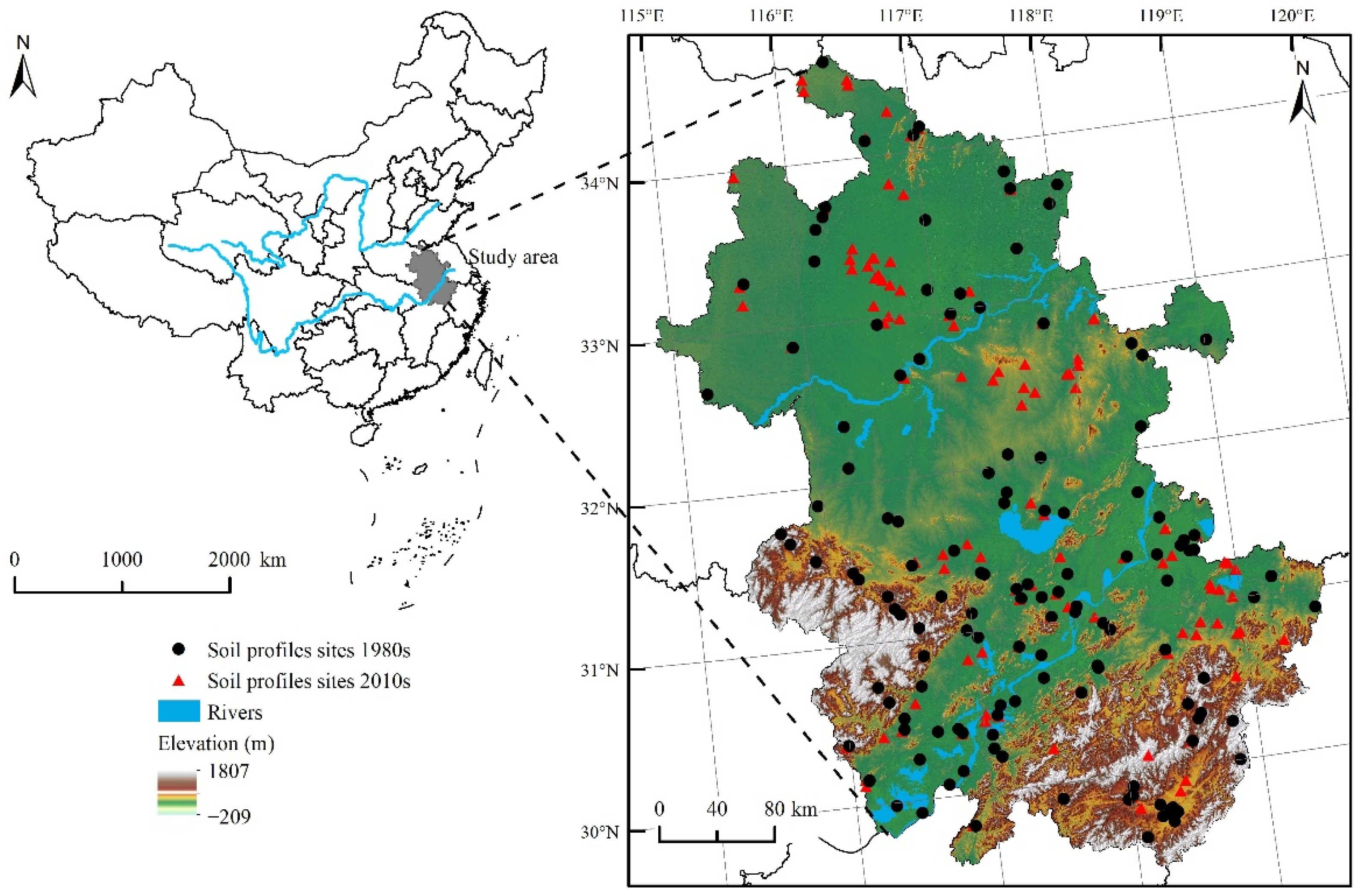
Figure 1. Location of the study area and the spatial distribution of soil profiles used in the study.
Remotesensing 15 05228 g001
Figure 2. Methodological flowchart for testing the hypothesis. Spatial laboratory soil spectral information was used as environmental covariates to form 3 groups of environmental covariate sets with conventional soil-forming factor variables and satellite remote sensing variables, respectively. The random forest model was used to test the improvement in laboratory soil spectral information on 3D digital soil mapping performance for 5 soil attributes at 5 different depths.
Remotesensing 15 05228 g002
Figure 3. Spatialized laboratory soil spectral bands at five depth intervals: (a) R band, (b) G band, (c) B band, (d) SW-NIR band, (e) MW-NIR band, (f) LW-NIR band.
Remotesensing 15 05228 g003
Figure 4. Pearson correlation matrices of five soil attributes with environmental covariates. pH, CEC, Silt, SOC and TP were the soil attributes used in this study. Abbreviations for conventional soil-forming variables and satellite remote sensing variables can be found in Table 2; R, G, B, SW-NIR, MW-NIR and LW-NIR were the laboratory soil spectral bands used in this study; T1–T12 for laboratory soil spectral information variables can be found in Table 3.
Remotesensing 15 05228 g004
Figure 5. R2 (left side) and RMSE (right side) improvements in 3D soil attribute mapping using satellite remote sensing information and laboratory soil spectral information, (a) pH, (b) CEC, (c) Silt, (d) SOC, (e) TP. The bars in the figure show R2 differences/improvements for different models; The broken line indicates a difference/improvement in the RMSE.
Remotesensing 15 05228 g005
Figure 6. The relative importance of environmental covariates for (a) pH, (b) CEC, (c) Silt, (d) SOC and (e) TP.
Remotesensing 15 05228 g006
Figure 7. Scatter plot of the relative importance percentage of laboratory soil spectral information variables against prediction accuracy improvement for C+LSS. (a) pH, (b) CEC, (c) Silt, (d) SOC and (e) TP.
Remotesensing 15 05228 g007
Figure 8. Scatter plot of the relative importance percentage of laboratory soil spectral information variables and prediction accuracy improvement for C+LSS. The red line is a linear regression fit based on partial least squares.
Remotesensing 15 05228 g008
Table 1. Statistical descriptions of the spline-fixed five soil attributes at different depths.
Soil AttributesDepth (cm)Mean (%)SD (%)CVSkewnessKurtosis
pH0–56.3851.2820.2010.437−0.908
5–156.4841.2210.1880.404−0.918
15–306.7571.1500.1700.045−0.993
30–606.9231.1360.164−0.247−0.924
60–1007.0341.1150.158−0.413−0.689
CEC0–515.5067.1470.4610.680−0.304
5–1515.1406.9090.4560.661−0.381
15–3014.6547.0870.4840.560−0.524
30–6015.2977.5060.4930.603−0.706
60–10015.0257.2030.4790.555−0.431
Silt0–534.12212.2520.3590.284−0.203
5–1534.11511.3260.3320.164−0.299
15–3033.86011.0320.3260.034−0.093
30–6033.49412.2090.3650.4031.441
60–10033.04812.2200.3700.0071.572
SOC0–515.89413.7180.8633.17412.864
5–1514.40711.4730.7962.82111.265
15–3010.6588.9960.8442.6169.790
30–607.52810.4991.3955.66643.163
60–1005.4997.0051.2745.27637.203
TP0–50.5570.3190.5732.0205.743
5–150.5490.2910.5301.6773.696
15–300.5290.3030.5732.58813.015
30–600.4740.2580.5441.9597.086
60–1000.4490.2640.5892.2409.941
Table 2. Original environmental covariates and their related information collected in this study.
CategoryCovariateDescriptionResolution
Parent materialpmclsType of parent materials90 m
TerrainelevElevation (m)90 m
anHisMountain shadow90 m
slpSlope (%)90 m
aspAspect (°)90 m
curPlnPlan curvature90 m
curPrfProfile curvature90 m
TWITopographic wetness index90 m
TPITopographic position index90 m
MrVBFMultiscale Valley flatness index90 m
MrRTFMultiscale ridge flatness index90 m
ClimateMATMean annual temperature (°C)1000 m
rangDiurnalMean diurnal range (°C)1000 m
rangAnnualMean annual range (°C)1000 m
isotherIsothermality (°C)1000 m
tempSeasonAir temperature seasonality (°C)1000 m
tempMaxWarmMaximum air temperature of warmest month (°C)1000 m
tempMinColdMinimum air temperature of coldest month (°C)1000 m
tempWettestAir temperature of wettest season (°C)1000 m
tempDriestAir temperature of driest season (°C)1000 m
tempMeanWarmMean air temperature of warmest month (°C)1000 m
tempMeanColdMean air temperature of coldest month (°C)1000 m
MAPMean annual precipitation (mm yr−1)1000 m
precSeasonPrecipitation seasonality (mm yr−1)1000 m
precWettestPrecipitation of wettest month (mm mh−1)1000 m
precDriestPrecipitation of driest month (mm mh−1)1000 m
precWarmPrecipitation of warmest month (mm mh−1)1000 m
precColdPrecipitation of coldest month (mm mh−1)1000 m
solarRedMean annual solar radiation (J m−2 yr−1)500 m
windSpeedWind speed (m s−1)1000 m
vaporPressWater vapor pressor (kpa)1000 m
evaTraTerrestrial evaporation500 m
LSTLand surface temperature (°C)500 m
BiologicalNDVIMean NDVI250 m
EVIMean EVI250 m
Satellite remote sensingMODISb1Reflectance of the red band (620–672 nm)500 m
MODISb2Reflectance of near-infrared short wave (841–890 nm)500 m
MODISb3Reflectance of the blue band (459–479 nm)500 m
MODISb4Reflectance of the green band (545–565 nm)500 m
MODISb5Reflectance of near-infrared medium wave (1230–1250 nm)500 m
MODISb6Reflectance of near-infrared medium wave (1628–1652 nm)500 m
MODISb7Reflectance of near-infrared long wave (2105–2155 nm)500 m
Table 3. The expressions of soil spectral correlation factors.
Soil Spectral Correlation FactorsComputed Expression
T1 R G
T2 R + G + S W N I R
T3 S W N I R R S W N I R + R
T4 G R G + R
T5 S W N I R G S W N I R + G
T6 R × G
T7 R 2 + G 2
T8 S W N I R L W N I R
T9 S W N I R M W N I R
T10 M W N I R G
T11 M W N I R R
T12 G R
Table 4. Accuracies of spatial predictions of six laboratory soil spectral bands at different depths.
Laboratory Soil Spectral BandsDepth (cm)MERMSER2CCC
R0–5−0.1292.9820.2090.436
5–15−0.0982.8900.2390.499
15–300.3412.9620.2790.477
30–60−0.0222.8070.3850.597
60–100−0.4802.8190.5180.687
G0–5−0.2612.7480.1420.398
5–15−0.3382.7020.1760.401
15–300.2512.4220.2240.449
30–600.3342.5640.2860.587
60–100−0.2032.4340.4260.584
B0–5−0.0171.8640.3310.520
5–15−0.0261.7470.3800.550
15–300.0641.7940.3490.498
30–60−0.0381.6800.3320.510
60–1000.0631.6080.4000.598
SW-NIR0–5−0.1822.7000.4040.586
5–15−0.1842.5380.4310.625
15–30−0.1062.1530.5150.515
30–600.1002.4230.5150.682
60–1000.0553.3580.4330.611
MW-NIR0–5−0.1823.4820.2790.405
5–15−0.8462.9460.4290.633
15–30−0.0934.1390.4990.669
30–60−0.3114.8290.4060.587
60–100−0.2085.1040.3710.559
LW-NIR0–5−0.3591.1130.4590.614
5–15−0.4244.1620.3940.543
15–30−0.2054.1740.4100.573
30–60−0.3474.4810.3950.564
60–100−0.3544.7690.3080.493
ME: mean error; RMSE: root mean square error; R2: coefficient of determination; CCC: concordance correlation coefficient.
Table 5. Significance tests of correlation coefficients between the soil attributes at different depths and satellite remote sensing waveband variables and laboratory soil spectral variables.
Soil AttributesDepth (cm)Satellite
Remote Sensing
Lab Soil Spectral
Information
p Value
pH0–50.186 ± 0.114 b0.364 ± 0.113 a0.021
5–150.117 ± 0.035 b0.305 ± 0.139 a0.034
15–300.117 ± 0.031 a0.285 ± 0.141 a0.058
30–600.158 ± 0.041 b0.313 ± 0.111 a0.030
60–1000.126 ± 0.007 b0.199 ± 0.058 a0.045
CEC0–50.036 ± 0.021 b0.165 ± 0.096 a0.035
5–150.053 ± 0.032 b0.182 ± 0.097 a0.038
15–300.052 ± 0.017 b0.145 ± 0.074 a0.044
30–600.079 ± 0.053 b0.167 ± 0.057 a0.022
60–1000.067 ± 0.071 b0.124 ± 0.039 a0.049
Silt0–50.026 ± 0.028 a0.049 ± 0.039 a0.343
5–150.025 ± 0.028 a0.045 ± 0.034 a0.352
15–300.074 ± 0.047 b0.177 ± 0.065 a0.017
30–600.050 ± 0.023 b0.152 ± 0.061 a0.012
60–1000.035 ± 0.041 b0.157 ± 0.065 a0.006
SOC0–50.094 ± 0.019 b0.249 ± 0.124 a0.049
5–150.122 ± 0.035 b0.225 ± 0.079 a0.042
15–300.108 ± 0.025 b0.203 ± 0.074 a0.045
30–600.112 ± 0.030 b0.177 ± 0.045 a0.017
60–1000.092 ± 0.055 b0.163 ± 0.061 a0.043
TP0–50.022 ± 0.033 b0.089 ± 0.035 a0.006
5–150.015 ± 0.020 b0.149 ± 0.063 a0.002
15–300.019 ± 0.005 b0.143 ± 0.090 a0.030
30–600.035 ± 0.025 b0.107 ± 0.050 a0.028
60–1000.127 ± 0.020 b0.187 ± 0.044 a0.029
Different lowercase letters indicate significant differences at p < 0.05 between the correlations of soil attributes with satellite remote sensing waveband variables and the correlations of laboratory soil spectral information variables.
Table 6. Average accuracy improvements in the five soil attributes at 0–60 cm and 60–100 cm depths when using satellite remote sensing variables and laboratory soil spectral variables.
Soil AttributesDepth (cm)Average of Accuracy Improvement
M_C+SRSM_C+LSS
pH0–600.2080.334
60–1000.1060.303
CEC0–600.1890.505
60–100−0.0380.867
Silt0–600.5230.633
60–1000.1540.260
SOC0–600.2900.411
60–1000.2230.479
TP0–600.2470.355
60–100−0.2390.379
Disclaimer/Publisher’s Note: The statements, opinions and data contained in all publications are solely those of the individual author(s) and contributor(s) and not of MDPI and/or the editor(s). MDPI and/or the editor(s) disclaim responsibility for any injury to people or property resulting from any ideas, methods, instructions or products referred to in the content.