A Multi-Stream Attention-Aware Convolutional Neural Network: Monitoring of Sand and Dust Storms from Ordinary Urban Surveillance Cameras

Abstract

Sand and dust storm (SDS) weather has caused several severe hazards in many regions worldwide, e.g., environmental pollution, traffic disruptions, and human casualties. Widespread surveillance cameras show great potential for high spatiotemporal resolution SDS observation. This study explores the possibility of employing the surveillance camera as an alternative SDS monitor. Based on SDS image feature analysis, a Multi-Stream Attention-aware Convolutional Neural Network (MA-CNN), which learns SDS image features at different scales through a multi-stream structure and employs an attention mechanism to enhance the detection performance, is constructed for an accurate SDS observation task. Moreover, a dataset with 13,216 images was built to train and test the MA-CNN. Eighteen algorithms, including nine well-known deep learning models and their variants built on an attention mechanism, were used for comparison. The experimental results showed that the MA-CNN achieved an accuracy performance of 0.857 on the training dataset, while this value changed to 0.945, 0.919, and 0.953 in three different real-world scenarios, which is the optimal performance among the compared algorithms. Therefore, surveillance camera-based monitors can effectively observe the occurrence of SDS disasters and provide valuable supplements to existing SDS observation networks.

1. Introduction

Sand and dust storms (SDS) are typical weather disasters caused by strong and turbulent winds entraining dust particles into the air, severely affecting the environment, agriculture, industry, and human health for a long time [1]. Central Asia, Northern Africa, the Middle East, North America, and Australia are considered the primary sources of SDSs worldwide during the spring, winter, and early summer [2]. Since the extensive losses and damage caused by SDS events, the early warning and monitoring of SDS have attracted considerable attention. As early as 2007, the World Meteorological Organization launched the Sand and Dust Storm Warning Advisory and Assessment System (https://public.wmo.int/en/our-mandate/focus-areas/environment/SDS/warnings) (accessed on 1 January 2023) to enhance the ability of global countries to deliver timely and quality SDS forecasts, observations, information, and knowledge to human beings [3]. After decades of efforts, several technologies or tools are available and can be classified as ground- and space-based monitoring technologies [4]. However, the rapid and small-scale characteristics of some SDS events pose challenges to the current monitoring system:

(1)

Traditional ground-based methods, like lookout towers, are considered more objective and directed observations. With advances in industrial manufacturing and sensing technologies, ground radars, lidars, and wireless sensor networks become essential options for SDS monitoring tasks while being irreplaceable parts in the calibration and integration of remote sensing-based measurements [2,5,6]. Limited by cost, operating requirements, and deployment conditions, these ground-based observations usually cannot be deployed at a high density over a large spatial scale, resulting in a lack of spatial representation of observation results.

(2)

Space-based technologies mainly refer to satellite-based remote sensing methods, which are important in monitoring, assessing, and predicting SDS events. The well-known Moderate Resolution Imaging Spectroradiometer (MODIS) and Total Ozone Mapping Spectrometer (TOMS) satellites [7] enable passive detection of the occurrence and transportation of an SDS on the vertical distribution, while Cloud-Aerosol Lidar and Infrared Pathfinder Satellite Observation (CALIPSO) satellites [8] can actively sense the vertical profile of cloud aerosols and inverse the vertical information of SDSs. However, the satellite is more suitable for large-scale and long-term SDS monitoring tasks. With the enhancement of satellite imagery resolution and the number of satellites, the problem of insufficient spatial and temporal resolution has been gradually alleviated. However, rapid sensing of small-scale dust storm events still needs to be improved.

The ground camera enables continuous recording of changes in the scene and rapid feedback on the emergence of SDSs, which researchers have noticed for its high temporal resolution observation advantage [5]. For example, Bukhari [9] attempted to use ground cameras to capture the startup phase of large-scale SDSs. In addition, some researchers have used what the cameras capture as evidence of dust storm events: Narasimhan and Nayar [10] analyzed the visual manifestations of haze and fog weather closer to SDSs and gave an essential reference for the visual-based SDS events identification and images reconstruction during SDS conditions; Chavez Jr et al. [11] deployed some cameras to take photos when the winds exceeded a pre-selected threshold to augment remote sensing satellites in order to enhance their capability of detecting SDSs; Dagsson-Waldhauserova et al. [12] combined images captured by surveillance cameras and portable dust measurement instruments to identify the extent, magnitude, and grain size characteristics of SDS events in southwestern Iceland; Urban et al. [13] used the images captured by ground remote cameras to estimate the amount and frequency of dust emissions from a setting in the Mojave Desert, USA. Although the above three works manually reviewing the imagery are practical, visually interpreting imagery is laborious, repetitive, and time-consuming, which could be more friendly to the operators, especially for long-term observations/images. To achieve automatic monitoring purposes, Gutierrez [6] proposed a feed-forward neural network for the automatic classification of SDS events from camera frames.

Generally, SDS videos/images captured by purposely placed surveillance cameras provide redundant ground-based observations serving to correct SDS information sensed by other means, such as space-based sensing results, and the potential of the surveillance camera network as a stand-alone SDS monitoring or early warning system needs to be further exploited. According to the authors, the reasons for this are the following: (1) The limited field of view dictates that ground cameras can detect SDSs at a small scale, but it is difficult to describe the full extent of large-scale SDSs. However, large-area deployment of cameras is costly, which is a bottleneck problem for ground camera-based SDS monitoring networks. (2) Existing ground camera-based SDS monitoring efforts are inadequately automated and still require high labor costs, while the complex and dynamic urban surveillance scenarios present further challenges to the accuracy of SDS detection algorithms, which require the development of algorithms specifically for SDS monitoring from surveillance cameras.

As the smart city develops, widespread surveillance cameras have become essential for traffic, security, emergency management, etc. According to the survey by Comparitech, approximately 770 million surveillance cameras are deployed worldwide (https://www.comparitech.com/) (accessed on 1 January 2023). Such a high-density surveillance camera network provides the hardware basis for high spatial resolution SDS observation; meanwhile, 4G/5G communication technology provides the software basis for high temporal resolution SDS video transmission. Therefore, in theory, surveillance cameras have great potential for high spatiotemporal resolution SDS event monitoring. On the other hand, with the development of deep learning technology, CNN-based algorithms have achieved satisfactory performance in object detection tasks, which brings new opportunities to surveillance camera-based SDS detectors. In such a context, we used deep learning to build a surveillance camera-based SDS monitor. The main contributions of this study are as follows:

(1)

The designed monitoring system is deployed on existing urban surveillance resources rather than specifically deploying cameras, thus having higher reliability and obvious low-cost advantages. To the best of our knowledge, prior efforts did not use ordinary urban surveillance cameras for such a task.

(2)

A novel Multi-Stream Attention-aware Convolutional Neural Network (MA-CNN) is proposed, which learns SDS image features at different scales through a multi-stream structure and employs the attention mechanism to achieve satisfactory performance for accurate and automatic SDS identification from complex and dynamic surveillance scenarios.

(3)

For deep learning model training and testing, sand and dust storm image (SDSI), a new dataset consisting of 13,216 images (6578 SDS images and 6638 non-SDS images taken from scenes similar to SDS scenarios), was constructed.

The rest of this paper is organized as follows: Following this introduction, we detail the proposed MA-CNN in Section 2; we discuss the experimental results in Section 3 and conclude in Section 4.

2. Methodology

Intuitively, SDS monitoring via surveillance cameras can be considered a typical object detection issue in computer vision, i.e., detecting the occurrence of SDSs from surveillance videos, which can be divided into two parts: selecting image features and constructing the detection algorithm. Both of the above two steps contribute to SDS detection performance.

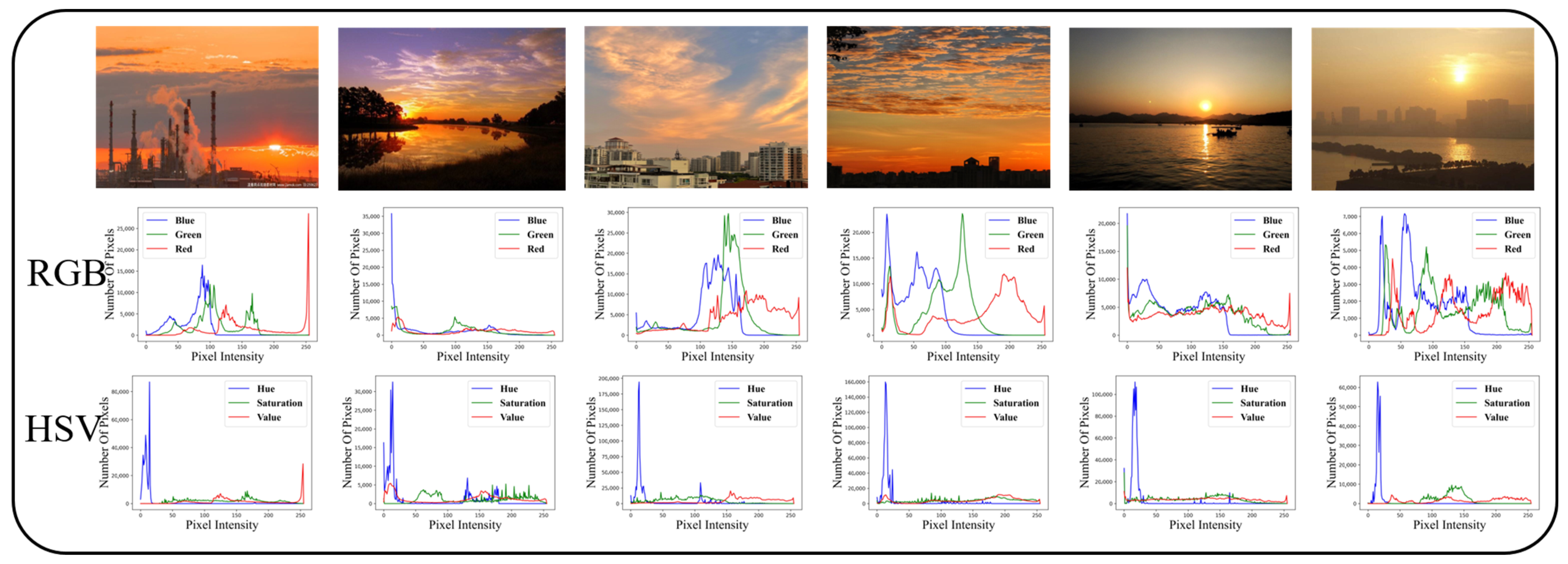
2.1. Image Features Selection

In meteorology, the definition of SDS weather levels is mainly based on horizontal visibility while referring to wind strength during SDS occurrences. A higher SDS level is associated with higher wind speed and lower visibility, and vice versa. It was observed that there were differences in the impact of different levels of SDS on surveillance images/videos.

For a lower-level SDS event, similar to fog, smog, and haze weather events, its appearance commonly causes a significant reduction in the sharpness and contrast of images captured by outdoor surveillance cameras, resulting in color shifting and missing detail problems [14]. The degradation effect caused by these weather events can be generically expressed as follows [10,15,16]:

$$Intensity\left(x\right)=J\left(x\right)t\left(x\right)+A(1-t(x\left)\right)$$

(1)

where $Intensity\left(x\right)$ is the observed intensity, $J\left(x\right)$ is the scene radiance, $A(\bullet )$ is the global atmospheric light, and $t\left(x\right)$ is the medium transmission describing the portion of the light that is not scattered and reaches the surveillance camera.

Previous studies have pointed out that the radius of particles in SDSs is close to 25 µm, which is much larger than that in haze (0.01–1 µm) and fog (1–10 µm) conditions [10,17]. Since particles of different sizes show varying reflection interactions with visible light, the degradation effects of SDS and the other three weather conditions differ slightly. Nevertheless, the generic model (i.e., Equation (1)) still works, so images taken in these environments are hard to discriminate.

Visually, these weather events change the color of the surveillance image. Researchers were quick to build single or multiple color channels (classical ones like dark channels [18]) that are sensitive to weather conditions, thus establishing a prior or assumption in terms of color space for fog, haze, smog, and SDS removal and image enhancement tasks. Single channels of RGB [19,20], HSV [21], and YIQ [22] color spaces are popular options. As shown in Figure 1, surveillance images captured under haze, fog, smog, and SDS weather conditions were randomly selected. Their effects on the surveillance images in HSV color space were compared. Figure 1 illustrates that the listed weather events blurred the natural images. Moreover, the Hue color channel exhibits a single-peak pattern in the weather-influenced images and can be considered as a color prior or assumption of these blurred images. To date, image deblurring algorithms still favor this strategy highly and have made significant progress [17,19,23,24].

In addition to the images taken during the above weather, we found that similar surveillance images also have single peaks in the Hue channel, as shown in Figure 2, making it more challenging to accurately distinguish SDSs in surveillance images.

Essentially, the purpose of the deblurring studies is to realize image restoration, which solves the problem of inconsistency between SDS images and the corresponding natural images. In contrast, our study focuses on monitoring the appearance of SDS via surveillance cameras. The crucial point is accurately distinguishing those surveillance scenarios that are similar to SDS. That is, sharing similar image characteristics with fog, haze, smog, etc., makes it more challenging to accurately distinguish SDS visually.

High-level SDS usually move fast together with low visibility. Here, a surveillance video recording the complete process of SDS from generation to transiting is collected, whose key frames are shown in Figure 3. While still using the image HSV color space as an example, it can be observed that as the SDS moves and the proportion of sand in the image changes, accompanied by changes in the characteristics of the HSV color space (for example, in the first two images the single-peak pattern of the Hue channel is not apparent). Therefore, the image features of high-level SDS events are dynamically changing, resulting in the fixed manual image features needing to be more manageable to describe thoroughly the randomly occurring SDS events in nature.

Given the dynamic behavior of SDSs and the high similarity of image features with relevant scenarios, constructing image features based on specific channels for a robust and accurate description of SDSs poses significant challenges. Inspired by [17], we consider the three channels (R, G, B) to be related and not independent. Therefore, taking the original image as an inseparable indivisibility in the form of a tensor for the input of the following detection algorithm.

2.2. Multi-Stream Attention-Aware CNN Network

As described in Section 2.1, how to detect the occurrence of SDSs from surveillance images, mainly to distinguish SDS events from similar scenarios, becomes a fundamental problem for a detector to solve. With the development of deep learning technology, CNN-based algorithms have achieved satisfactory performance in object detection and classification tasks, bringing new opportunities to construct surveillance camera-based SDS detectors. On the other hand, inspired by the biological systems of humans that tend to focus on the distinctive parts when processing large amounts of information, the attention mechanism has the advantage of solving the problem of information overload and improving the accuracy of results [25,26]. As one of the latest advancements in deep learning, the attention mechanism has become an essential tool in deep learning [27,28].

In this section, the attention mechanism is employed to locate the most salient components of the feature maps in CNNs and to remove the redundancy. Then, a Multi-Stream Attention-aware CNN Network (MA-CNN) is proposed for SDS detection from surveillance images, as shown in Figure 4. In MA-CNNs, the input data are simultaneously fed into multiple streams with different scales. In each stream, the features acquired by the stacked 2D CNN layers are fed into the spatial attention layer to acquire more focused SDS-sensitive features. Then the two layers are concatenated as input to a deeper layer.

Considering a CNN with $L$ layers, the hidden state of layer $l$ is represented as $H_l$, where $lϵ\{\mathrm{1,2}\dots ,L\}$. In this notation, the input image can be defined as $H_1$. The convolutional layer consists of two parts learnable parameters, that is, the weight matrix $W_l$ that connects layer $l$ and layer $l-1$ and the bias term vector $b_l$. Hence, each neuron in convolutional layer $l$ is only connected with a local region on $H_{l-1}$ and $W_l$ is shared among all spatial locations. In order to improve translation invariance and representation capability, convolutional layers are interleaved with point-wise nonlinearity (i.e., Leaky ReLU, whose parameter alpha = 0.1 [29]) and nonlinear down-sampling operation (i.e., 2D max pooling). The feature map of $l$ can be obtained by the following:

$$F_1=Max\_pooling(Leaky\_ReLU\left(H_{ l-1 }\ast W_l+b_l\right)), l=\mathrm{1,2},\dots ,L$$

(2)

where $\ast$ denotes the 2D convolution operation.

As shown in Figure 4, in order to enable the proposed network to learn richer semantic representations of the input image progressively, the number of channels in the outputs of successive blocks gradually increases as 64 → 128 → 256 → 512, and the kernel size of the connects layer gradually increases as 3 × 3 → 5 × 5 → 7 × 7. We integrate an attention mechanism [30] into each stream. As described in Section 3.1, considering the high similarity between SDSs and other monitoring scenarios (e.g., fog, smog, and haze), we introduce spatial attention mechanism to adaptively bootstrap features related to the key SDS-relevant features and pay less attention to those less feature-rich regions. The features obtained from the spatial attention layer and the last CNN layer are then concatenated as the final vectors of each stream. The details of the spatial attention mechanism are shown in Figure 5.

For an input feature $F$ with a size of $\mathrm{H}\times \mathrm{W}\times \mathrm{C}$, firstly, the spatial information of a 2D feature map is generated by the average pooling feature ($F_{avg}\mathsf{ϵ}{R}^{l\times H\times W}$) and max pooling feature ($F_{max}\mathsf{ϵ}{R}^{l\times H\times W}$), respectively. Then, $F_{avg}$ and $F_{max}$ are concatenated and convolved by a standard convolution layer, producing a 2D spatial attention feature map $M_F\left(S^{\prime }\right)\mathsf{ϵ}{R}^{H\times W}$. The spatial attention is computed as follows:

$$M_F\left(S^{\prime }\right)=\delta \left(f^{7\times 7}\right([avg\_pooling\left(F\right);\mathrm{m}\mathrm{a}\mathrm{x}\_pooling(F\left)\right]\left)\right)=\delta \left(f^{7\times 7}\right([F_{avg};F_{avg}]\left)\right)$$

(3)

where $\delta (\bullet )$ denotes the sigmoid function and $f^{7\times 7}(\bullet )$ means the convolution operation with the filter size of 7 × 7.

Moreover, to mitigate overfitting, the 0.5 via spatialdropout2D [31] is added to each stream’s second and last layers. Then, the feature responses from three streams are concatenated and fed into a GlobalAveragePooling2D output layer to produce the final vectors. Lastly, a fully connected layer with a size of 512 and a Softmax classifier can be utilized for a two-class classification.

2.3. Experiment Setup

2.3.1. Experimental Environment

Our experiments were performed on a workstation with Ubuntu 11.2.0 (Linux 5.15.0-25-generic) for the operating system. More specifications are as follows:

• 2× Intel Xeon Silver 4216 [email protected] GHz (32 cores);
• 8×NVIDIA GEFORCE GTX2080Ti graphics cards equipped with 11 GB GDDR6 memory;
• 188 GB RAM;
• Python 3.9.16;
• TensorFlow 2.4.1, Scikit-learn 1.2.1, and Keras 2.4.3 libraries;
• CUDA 11.8 and CUDNN 8.

2.3.2. Evaluation Metrics

The performance of SDS detection algorithms is evaluated by the weighted Precision, weighted Recall, and weighted F1 score, which are calculated as follows:

$$\mathrm{P}\mathrm{r}\mathrm{e}\mathrm{c}\mathrm{i}\mathrm{s}\mathrm{i}\mathrm{o}\mathrm{n}={\displaystyle {\sum }_{\mathrm{i}=1}^{\mathrm{n}}}\frac{\mathrm{T}{\mathrm{P}}_{\mathrm{i}}}{(\mathrm{T}{\mathrm{P}}_{\mathrm{i}}+\mathrm{F}{\mathrm{P}}_{\mathrm{i}})}\times {\mathrm{r}}_{\mathrm{i}}$$

(4)

$$\mathrm{R}\mathrm{e}\mathrm{c}\mathrm{a}\mathrm{l}\mathrm{l}={\displaystyle {\sum }_{\mathrm{i}=1}^{\mathrm{n}}}\frac{\mathrm{T}{\mathrm{P}}_{\mathrm{i}}}{(\mathrm{T}{\mathrm{P}}_{\mathrm{i}}+\mathrm{F}{\mathrm{N}}_{\mathrm{i}})}\times {\mathrm{r}}_{\mathrm{i}}$$

(5)

$$\mathrm{F}1\_\mathrm{s}\mathrm{c}\mathrm{o}\mathrm{r}\mathrm{e}={\displaystyle {\sum }_{\mathrm{i}=1}^{\mathrm{n}}}2\times \frac{{\mathrm{p}\mathrm{r}\mathrm{e}\mathrm{c}\mathrm{i}\mathrm{s}\mathrm{i}\mathrm{o}\mathrm{n}}_{\mathrm{i}}·{\mathrm{r}\mathrm{e}\mathrm{c}\mathrm{a}\mathrm{l}\mathrm{l}}_{\mathrm{i}}}{{\mathrm{p}\mathrm{r}\mathrm{e}\mathrm{c}\mathrm{i}\mathrm{s}\mathrm{i}\mathrm{o}\mathrm{n}}_{\mathrm{i}}+{\mathrm{r}\mathrm{e}\mathrm{c}\mathrm{a}\mathrm{l}\mathrm{l}}_{\mathrm{i}}}\times {\mathrm{r}}_{\mathrm{i}}$$

(6)

where $\mathrm{T}\mathrm{P}$ is the number of true positives; $\mathrm{F}\mathrm{P}$ is the number of false positives; $\mathrm{F}\mathrm{N}$ is the number of true negatives; i is the class index; and ${\mathrm{r}}_{\mathrm{i}}$ is the ratio between the number of samples of class i and the total number of samples in all classes.

2.3.3. Dataset Building

For the training and testing of the deep learning model, we constructed a dataset called sand and dust storm image (SDSI). As described in Section 3.1, surveillance images obtained between smog, fog, and haze weather conditions and SDSs are easily confused. Therefore, fog and haze images were collected as negative samples. Furthermore, it was observed that scenes such as sunset, sunrise, rainy weather, and smoke in everyday life also have a relatively high similarity to SDS, as shown in Figure 6d–g; thus, images of these scenes were also collected as part of the negative samples.

To ensure the number and diversity of the constructed SDSI dataset, images searched from the Internet and captured by surveillance cameras were jointly used. Finally, the positive samples (labeled as “Sandstorm”) comprised 6578 images of SDSs taken in various scenarios. In comparison, 6638 images with similar scenarios to SDS conditions were taken to form the negative samples (labeled as “Others”). After that, the obtained images were split into training, validation, and test datasets, as shown in

Table 1. Definition of Training-Test-Validation Split.

	Training Dataset	Validation Dataset	Test Dataset	Total
Other	4431	1029	1178	6638
Sandstorm	4425	1028	1125	6578
Total	8856	2057	2303	13,216

.

2.3.4. Model Training

Employing accuracy as a metric, all algorithm/model training is performed by minimizing the categorical cross-entropy loss with the Adam optimizer (${\mathsf{\beta }}_1=0.99,{\mathsf{\beta }}_2=0.999$). Moreover, the learning rate is set to 0.0001 and the batch size is set to 16. We trained each algorithm from 100 to 300 epochs until a stable result is obtained. The models were evaluated with a K-fold cross-validation scheme in our SDSI dataset ($\mathrm{K}=10$).

3. Results

3.1. Experiments in SDSI Dataset

To further evaluate the effectiveness of our proposed CNNs, nine well-known and commonly used deep learning models for object detection tasks, i.e., VGG16 and VGG19 [32], NasNetMobile [33], Xception [34], ResNet50 [35], Mobile Net and Mobile Net V2 [36], InceptionV3 [37], and DenseNet121 [38], are selected for comparison. The performance of different algorithms in the SDSI dataset (test dataset) is shown in

Table 2. Performance of different algorithms in the SDSI dataset.

	Precision	F1_Score	Recall	Parameters
VGG16	0.830	0.864	0.858	14,715,714
VGG19	0.834	0.829	0.830	20,025,410
NasNetMobile	0.778	0.833	0.820	4,271,830
Xception	0.771	0.852	0.834	20,865,578
ResNet50	0.736	0.633	0.677	23,591,810
Mobile Net V1	0.693	0.814	0.774	3,230,914
Mobile Net V2	0.788	0.854	0.840	2,260,546
InceptionV3	0.800	0.850	0.840	21,806,882
DenseNet121	0.802	0.867	0.855	7,039,554
MA-CNN (Ours)	0.857	0.868	0.866	28,171,314

Note: The best results are highlighted in bold.

.

Evaluated on the SDSI dataset, the proposed MA-CNN achieves state-of-the-art performance regarding Precision (0.857), F1 _Score (0.868), and Recall (0.866), as shown in Table 2. In general, MA-CNN shows significant improvement in precision than the compared methods. VGG16 and DenseNet121 performed closer to the proposed method in the F1 _Score and Recall metrics but with approximately 2.7% and 5.5% less than the proposed method in precision, respectively.

Considering that the spatial attention mechanism has good generality for existing deep learning networks, it was added before the output layer of the selected nine comparison algorithms. The spatial attention layer is added before the first fully connected layer for VGG16, VGG19, ResNet50, and Mobile Net V1. In contrast, for InceptionV3, Xception, NasNetMobile, and DenseNet121, the spatial attention layer is added after the last concated layer. For Mobile Net V2, the spatial attention layer is added after the last bottleneck). Taking VGG16 as an example, the structure of VGG16 with the spatial attention mechanism is labeled as “VGG16-A”. Analogously, nine other comparison algorithms with the attention mechanism were obtained. The performance of different algorithms with spatial attention mechanisms in the SDSI dataset (test dataset) is presented in

Table 3. Performance of different algorithms in the SDSI dataset after spatial attention mechanisms were added.

	Precision	F1_Score	Recall	Parameters
VGG16	0.812	0.855	0.847	14,781,924
VGG19	0.821	0.847	0.842	20,091,620
NasNetMobile	0.801	0.861	0.861	4,551,802
Xception	0.774	0.844	0.828	21,916,458
ResNet50	0.704	0.642	0.670	24,642,690
Mobile Net V1	0.799	0.854	0.852	3,494,210
Mobile Net V2	0.732	0.822	0.796	2,671,586
InceptionV3	0.786	0.835	0.824	22,857,762
DenseNet121	0.790	0.858	0.845	7,039,554
MA-CNN (Ours)	0.857	0.868	0.866	28,171,314

Note: The best results are highlighted in bold.

.

Table 3 suggests that our proposed algorithm achieves optimal performance after adding the attention mechanism. Comparing Table 2 and Table 3, the performance of VGG16, Mobile Net V2, Inception V3, and DenseNet121 algorithms decreased after the attention layers were added. In summary, the attention mechanism is unsuitable for all the comparing deep learning models when detecting SDS via the SDSI dataset. However, Table 2 and Table 3 indicate that our proposed algorithm contains the maximum number of parameters compared to the other listed algorithms, resulting in the MA-CNN model taking more extended time in the training process.

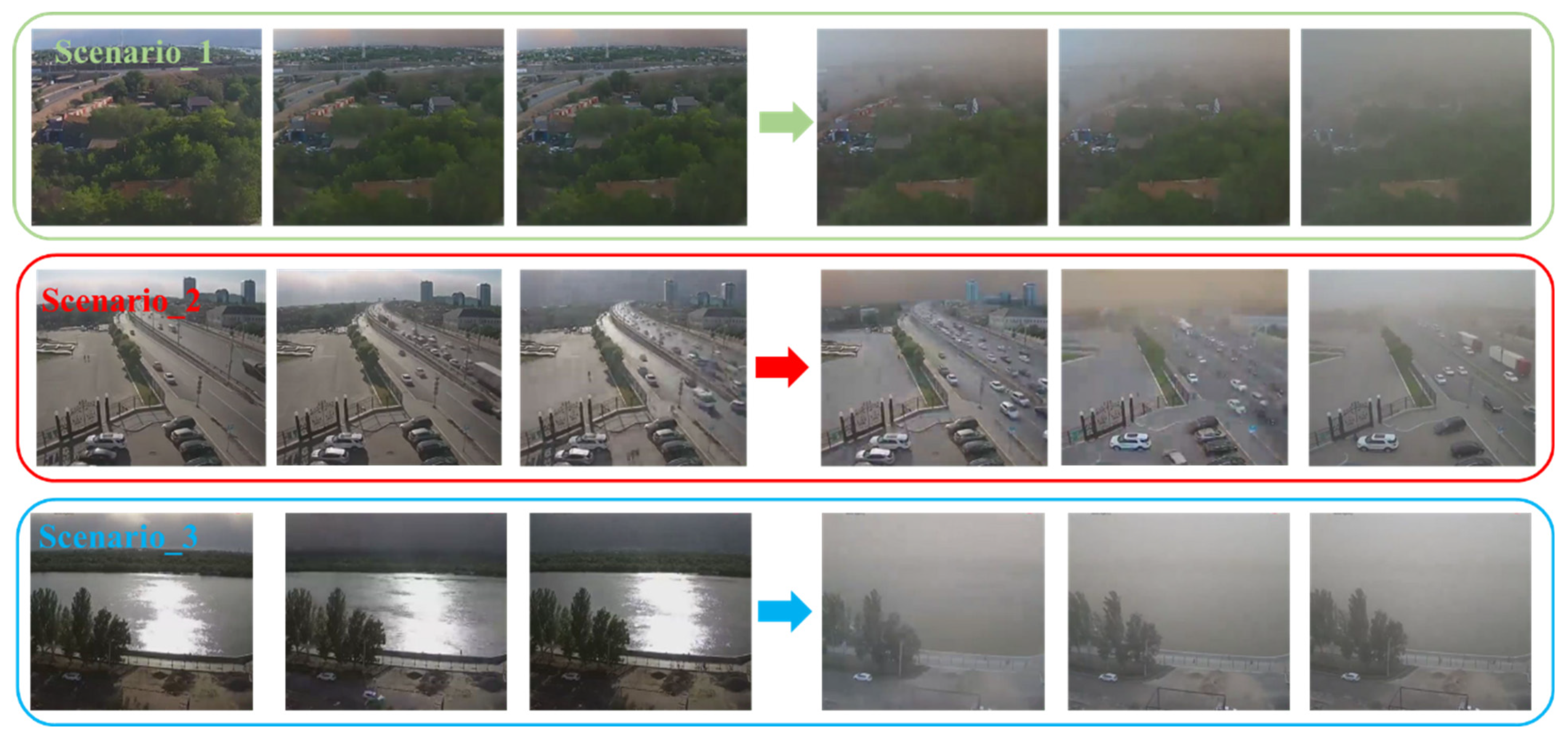
3.2. Experiments in Real-World Scenarios

Next, we evaluate the performance of the different SDS monitor algorithms in a real-world surveillance scenario. As shown in Figure 7, three surveillance videos that recorded the SDS from its appearance in the distance to its passage through the filming site were selected. Each video was fed into the SDS monitor algorithms in the form of a single frame. In the end, scenario_1 produced 375 images, while that of scenario_2 and scenario_3 were 241 and 282, respectively.

The experiment results of the three abovementioned real-world surveillance scenarios are reported in

Table 4. Performance of different algorithms in real-world surveillance scenario_1.

	Precision	F1_Score	Recall
VGG16	0.86	0.883	0.902
VGG19	0.891	0.912	0.925
NasNetMobile	0.925	0.936	0.957
Xception	0.887	0.892	0.865
ResNet50	0.785	0.832	0.804
Mobile Net V1	0.742	0.788	0.769
Mobile Net V2	0.924	0.939	0.94
InceptionV3	0.879	0.886	0.897
DenseNet121	0.897	0.913	0.944
MA-CNN (Ours)	0.945	0.967	0.956

Note: The best results are highlighted in bold.

,

Table 5. Performance of different algorithms in real-world surveillance scenario_2.

	Precision	F1_Score	Recall
VGG16	0.823	0.835	0.870
VGG19	0.856	0.894	0.908
NasNetMobile	0.842	0.851	0.850
Xception	0.822	0.817	0.834
ResNet50	0.771	0.820	0.799
Mobile Net V1	0.692	0.722	0.743
Mobile Net V2	0.870	0.895	0.913
InceptionV3	0.887	0.913	0.920
DenseNet121	0.906	0.923	0.926
MA-CNN (Ours)	0.919	0.936	0.934

Note: The best results are highlighted in bold.

and

Table 6. Performance of different algorithms in real-world surveillance scenario_3.

	Precision	F1_Score	Recall
VGG16	0.764	0.792	0.800
VGG19	0.902	0.933	0.941
NasNetMobile	0.910	0.934	0.922
Xception	0.861	0.823	0.842
ResNet50	0.845	0.883	0.871
Mobile Net V1	0.797	0.811	0.826
Mobile Net V2	0.853	0.892	0.887
InceptionV3	0.915	0.935	0.946
DenseNet121	0.922	0.971	0.957
MA-CNN (Ours)	0.953	0.967	0.948

Note: The best results are highlighted in bold.

.

Table 4 shows that, in surveillance scenario_1, the proposed algorithm achieves a Precision of 0.945 and an F1 _Score of 0.967, which is the highest among the listed algorithms; although NasNet has the highest Recall of 0.957, this is only 0.001 higher than that of our proposed MA-CNN; Table 5 illustrates that the MA-CNN achieved the best performance in surveillance scenario_2 with a Precision, F1 _Score, and Recall of 0.919, 0.936, and 0.934, respectively; Table 6 demonstrates that in surveillance scenario_3, DenseNET achieves the maximum values of F1 _Score and Recall, 0.971 and 0.955, which are 0.004 and 0.009 higher than the algorithm proposed in this paper, respectively; however, in terms of accuracy, the algorithm in this paper achieves the optimal performance of 0.953, which is 0.031 higher than DenseNet. The proposed MA-CNN performs stable and well for SDS monitoring in the above three real-world surveillance scenarios and can be considered the optimal model.

After that, the performance of different algorithms with spatial attention mechanisms in the three real-world surveillance scenarios was also used for comparison, as presented in

Table 7. Performance of different algorithms in real-world surveillance scenario_1 after spatial attention mechanisms were added.

	Precision	F1_Score	Recall
VGG16	0.875	0.891	0.884
VGG19	0.912	0.918	0.914
NasNetMobile	0.864	0.859	0.862
Xception	0.824	0.83	0.832
ResNet50	0.812	0.809	0.822
Mobile Net V1	0.787	0.789	0.792
Mobile Net V2	0.933	0.944	0.938
InceptionV3	0.902	0.911	0.907
DenseNet121	0.919	0.923	0.954
MA-CNN (Ours)	0.945	0.967	0.956

Note: The best results are highlighted in bold.

,

Table 8. Performance of different algorithms in real-world surveillance scenario_2 after spatial attention mechanisms were added.

	Precision	F1_Score	Recall
VGG16	0.852	0.859	0.862
VGG19	0.873	0.889	0.878
NasNetMobile	0.792	0.783	0.801
Xception	0.754	0.753	0.759
ResNet50	0.742	0.732	0.753
Mobile Net V1	0.725	0.737	0.734
Mobile Net V2	0.798	0.803	0.808
InceptionV3	0.907	0.915	0.918
DenseNet121	0.916	0.917	0.917
MA-CNN (Ours)	0.919	0.936	0.934

Note: The best results are highlighted in bold.

and

Table 9. Performance of different algorithms in real-world surveillance scenario_3 after spatial attention mechanisms were added.

	Precision	F1_Score	Recall
VGG16	0.814	0.807	0.815
VGG19	0.917	0.923	0.921
NasNetMobile	0.922	0.913	0.917
Xception	0.87	0.863	0.872
ResNet50	0.817	0.823	0.821
Mobile Net V1	0.825	0.818	0.834
Mobile Net V2	0.914	0.925	0.917
InceptionV3	0.929	0.933	0.952
DenseNet121	0.928	0.944	0.953
MA-CNN (Ours)	0.953	0.967	0.948

Note: The best results are highlighted in bold.

.

Table 7, Table 8 and Table 9 show that the MA-CNN still achieves optimal performance compared to other algorithms with spatial attention mechanisms. In addition, the accuracy of some comparison algorithms after the spatial attention mechanism was added shows a certain degree of degradation in real-world surveillance scenarios; for example, in surveillance scenarios 2 and 3, the Resnet50 algorithm shows a degradation in accuracy of 0.029 and 0.028 (please see Table 5, Table 6, Table 8 and Table 9). This phenomenon also occurs on the SDSI dataset, further indicating that the spatial attention mechanism is not suitable to be added to all deep learning algorithms.

For a more intuitive understanding of the SDS recognition pattern of the proposed algorithm, we compare the attention feature maps extracted by different deep learning algorithms shown in

Table A1. Attention feature maps extracted by different deep learning algorithms.

Images from scenario_1
VGG16
VGG19
NasNet
Xception
ResNet50
Mobile Net V1
MobileNet V2
InceptionV3
DenseNet121
MA-CNN (Ours)

and

Table A2. Attention feature maps extracted by different deep learning algorithms after attention mechanism.

Images from scenario_1
VGG16
VGG19
NasNet
Xception
ResNet50
Mobile Net V1
MobileNet V2
InceptionV3
DenseNet121
MA-CNN (Ours)

(Please see Appendix A). In Table A1 and Table A2, the first row show four SDS figures randomly selected from surveillance scenario_1, and from the second row onwards, the corresponding attention maps extracted by different algorithms are presented.

In the first two images, the SDS appears in the upper area of the surveillance images, correctly identified by most comparison algorithms. For the last two images, when the SDS is diffused throughout the image, more significant uncertainty emerges in the performance of different comparison algorithms. In contrast, Table A1 and Table A2 demonstrate that, in the four selected images, the attention feature maps of our MA-CNN method can match well with the changes of the pixels blurred by SDS, which indicates that the MA-CNN can identify and localize the SDSs that appear in the surveillance scenarios well. The visualization results further indicate that the proposed MA-CNN algorithm is more suitable for SDS monitoring via surveillance cameras.

4. Discussion

Compared to existing studies, the main contribution of our study is the use of surveillance cameras for SDS monitoring tasks, which sheds light on building a low-cost, high temporal and spatial resolution SDS monitoring network based on existing urban surveillance resources. However, some shortcomings need to be addressed.

(1)

Although the proposed MA-CNN model brings an improvement in SDS accuracy, it suffers from a long computational delay due to a relatively large number of parameters (as presented in Table 2 and Table 3). Taking the experimental platform shown in Section 2.3.1 as an example, the MA-CNN algorithm costs 0.78 s to judge whether an SDS appears in a surveillance image with a resolution of 1920 × 1080, whereas VGG16, VGG19, NasNetMobile, Xception, ResNet50, Mobile Net V1, Mobile Net V2, InceptionV3, and DenseNet121 take 0.39 s, 0.52 s, 0.27 s, 0.54 s, 0.65 s, 0.25 s, 0.21 s, 0.62 s, and 0.44 s, respectively. In practical applications, increasing the computational capability of the hardware devices or adopting a distributed computing manner are alternative solutions to reduce the abovementioned latency.

(2)

In this study, we detect SDSs in visible light surveillance video captured during the daytime, while in low-light scenarios such as nighttime, it is difficult to capture the appearance of an SDS in visible light surveillance video, and the MA-CNN method will on not work. Extensive research has shown that ordinary surveillance cameras can have “night vision” through near-infrared (NIR) video to perceive low-light scenarios [39], which provides the opportunity to monitor SDSs at night. Research on NIR video-based SDS monitoring, thereby constructing an all-weather observation system, will be the focus of the next step.

(3)

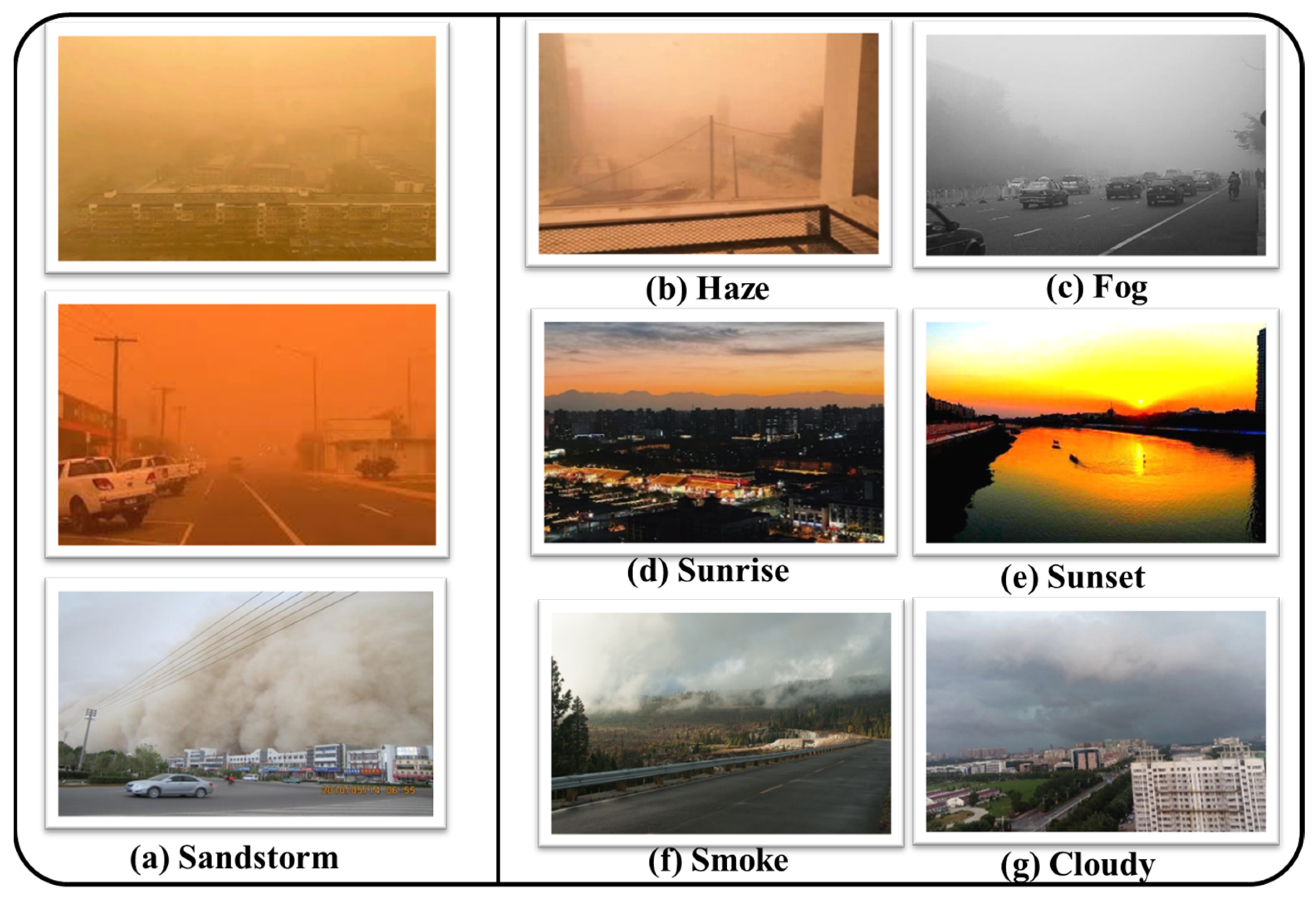
Rapid changes over time are an important distinction between SDSs and similar weather events (e.g., fog, haze, and smoke). Understanding SDSs from both temporal and spatial dimensions is an effective strategy to improve SDS monitoring accuracy. The proposed MA-CNN algorithm can mine the image features of SDSs from the spatial dimension, and the patterns of SDSs in the temporal dimension are not utilized. The main reason is that few dust storm videos can be collected currently, making it challenging to build a deep learning dataset for describing an SDS’s spatial and temporal features. Therefore, more SDS and similar weather video data should be collected in the future, which is the basis for the study of more accurate SDS monitoring methods.

5. Conclusions

In this paper, we attempt to build urban surveillance cameras as SDS monitors. After analyzing the image features of SDSs, RGB images were selected as the input of the recognition algorithm; attentive mechanisms were introduced, and a deep learning model named MA-CNN was proposed for the accurate discrimination of SDSs via surveillance images. In addition, the SDSI dataset was constructed for the training and testing of the model. The experimental results on the SDSI dataset show that compared with 18 related deep learning algorithms, the MA-CNN model achieves the best performance with a precision, F1_score, and recall of 0.857, 0.868, and 0.866, respectively. Moreover, the performance on three real-world surveillance scenarios also demonstrates that the MA-CNN can effectively identify an SDS’s occurrence in surveillance images. The constructed SDS monitor can be deployed on existing urban surveillance resources, which has the advantage of a low cost and provides a promising means for high spatiotemporal resolution SDS observation.

However, the monitors proposed in this study can only determine the occurrence of SDS events, resulting in limited practical value. Quantifying SDS levels from surveillance images or videos will be our focus in the future.

References

1. Shepherd, G.; Terradellas, E.; Baklanov, A.; Kang, U.; Sprigg, W.; Nickovic, S.; Boloorani, A.D.; Al-Dousari, A.; Basart, S.; Benedetti, A. Global Assessment of Sand and Dust Storms; United Nations Environment Programme: Nairobi, Kenya, 2016. [Google Scholar]
2. Jiao, P.; Wang, J.; Chen, X.; Ruan, J.; Ye, X.; Alavi, A.H. Next-Generation Remote Sensing and Prediction of Sand and Dust Storms: State-of-the-Art and Future Trends. Int. J. Remote Sens. 2021, 42, 5277–5316. [Google Scholar]
3. Nickovic, S.; Agulló, E.C.; Baldasano, J.M.; Terradellas, E.; Nakazawa, T.; Baklanov, A. Sand and Dust Storm Warning Advisory and Assessment System (Sds-Was) Science and Implementation Plan: 2015–2020; World Meteorological Organization: Geneva, Switzerland, 2015. [Google Scholar]
4. Behzad, R.; Barati, S.; Goshtasb, H.; Gachpaz, S.; Ramezani, J.; Sarkheil, H. Sand and Dust Storm Sources Identification: A Remote Sensing Approach. Ecol. Indic. 2020, 112, 106099. [Google Scholar]
5. Muhammad, A.; Sheltami, T.R.; Mouftah, H.T. A Review of Techniques and Technologies for Sand and Dust Storm Detection. Rev. Environ. Sci. Bio Technol. 2012, 11, 305–322. [Google Scholar]
6. Gutierrez, J. Automated Detection of Dust Storms from Ground-Based Weather Station Imagery Using Neural Network Classification. Ph.D. Thesis, New Mexico State University, Las Cruces, NM, USA, 2020. [Google Scholar]
7. McPeters, R.D. Nimbus-7 Total Ozone Mapping Spectrometer (Toms) Data Products User’s Guide; National Aeronautics and Space Administration, Scientific and Technical: Washington, DC, USA, 1996; Volume 1384. [Google Scholar]
8. Sassen, K.; Wang, Z.; Liu, D. Global Distribution of Cirrus Clouds from Cloudsat/Cloud-Aerosol Lidar and Infrared Pathfinder Satellite Observations (Calipso) Measurements. J. Geophys. Res. Atmos. 2008, 113, D00A12. [Google Scholar]
9. Bukhari, S.A. Depicting Dust and Sand Storm Signatures through the Means of Satellite Images and Ground-Based Observations for Saudi Arabia. PhD Thesis, University of Colorado at Boulder, Boulder, CO, USA, 1993. [Google Scholar]
10. Narasimhan, S.G.; Nayar, S.K. Vision and the Atmosphere. Int. J. Comput. Vis. 2002, 48, 233. [Google Scholar] [CrossRef]
11. Jr, C.; Pat, S.; Mackinnon, D.J.; Reynolds, R.L.; Velasco, M. Monitoring Dust Storms and Mapping Landscape Vulnerability to Wind Erosion Using Satellite and Ground-Based Digital Images. Arid. Lands. Newsl. 2002, 51, 1–8. [Google Scholar]
12. Dagsson-Waldhauserova, P.; Magnusdottir, A.Ö.; Olafsson, H.; Arnalds, O. The Spatial Variation of Dust Particulate Matter Concentrations During Two Icelandic Dust Storms in 2015. Atmosphere 2016, 7, 77. [Google Scholar] [CrossRef]
13. Urban, F.E.; Goldstein, H.L.; Fulton, R.; Reynolds, R.L. Unseen Dust Emission and Global Dust Abundance: Documenting Dust Emission from the Mojave Desert (USA) by Daily Remote Camera Imagery and Wind-Erosion Measurements. J. Geophys. Res. Atmos. 2018, 123, 8735–8753. [Google Scholar]
14. Abdulameer, F.S. Using Color Spaces Hsv, Yiq and Comparison in Analysis Hazy Image Quality. Adv. Phys. Theor. Appl 2019, 76, 15–23. [Google Scholar]
15. Fattal, R. Single Image Dehazing. ACM Trans. Graph. (TOG) 2008, 27, 1–9. [Google Scholar] [CrossRef]
16. Narasimhan, S.G.; Nayar, S.K. Chromatic Framework for Vision in Bad Weather. In Proceedings of the IEEE Conference on Computer Vision and Pattern Recognition, CVPR 2000 (Cat. No. PR00662), Hilton Head, SC, USA, 15 June 2000. [Google Scholar]
17. Xu, G.; Wang, X.; Xu, X. Single Image Enhancement in Sandstorm Weather Via Tensor Least Square. IEEE/CAA J. Autom. Sin. 2020, 7, 1649–1661. [Google Scholar] [CrossRef]
18. Sun, K.J.; Tang, X. Single Image Haze Removal Using Dark Channel Prior. IEEE Trans. Pattern Anal. Mach. Intell. 2010, 33, 2341–2353. [Google Scholar]
19. Cheng, Y.; Jia, Z.; Lai, H.; Yang, J.; Kasabov, N.K. Blue Channel and Fusion for Sandstorm Image Enhancement. IEEE Access 2020, 8, 66931–66940. [Google Scholar] [CrossRef]
20. Shi, F.; Jia, Z.; Lai, H.; Kasabov, N.K.; Song, S.; Wang, J. Sand-Dust Image Enhancement Based on Light Attenuation and Transmission Compensation. Multimed. Tools Appl. 2023, 82, 7055–7077. [Google Scholar] [CrossRef]
21. Fu, X.; Huang, Y.; Zeng, D.; Zhang, X.-P.; Ding, X. A Fusion-Based Enhancing Approach for Single Sandstorm Image. In Proceedings of the 2014 IEEE 16th International Workshop on Multimedia Signal Processing (MMSP), Jakarta, Indonesia, 22–24 September 2014. [Google Scholar]
22. Lee, H.S. Efficient Sandstorm Image Enhancement Using the Normalized Eigenvalue and Adaptive Dark Channel Prior. Technologies 2021, 9, 101. [Google Scholar] [CrossRef]
23. Ding, B.; Zhang, R.; Xu, L.; Cheng, H. Sand-Dust Image Restoration Based on Gray Compensation and Feature Fusion. Acta Armamentarii 2022. [Google Scholar] [CrossRef]
24. Gao, G.; Lai, H.; Liu, Y.; Wang, L.; Jia, Z. Sandstorm Image Enhancement Based on Yuv Space. Optik 2021, 226, 165659. [Google Scholar] [CrossRef]
25. Brauwers, G.; Frasincar, F. A General Survey on Attention Mechanisms in Deep Learning. IEEE Trans. Knowl. Data Eng. 2021, 35, 3279–3298. [Google Scholar]
26. Hassanin, M.; Anwar, S.; Radwan, I.; Khan, F.S.; Mian, A. Visual Attention Methods in Deep Learning: An in-Depth Survey. arXiv 2022, arXiv:2204.07756. [Google Scholar]
27. Niu, Z.; Zhong, G.; Yu, H. A Review on the Attention Mechanism of Deep Learning. Neurocomputing 2021, 452, 48–62. [Google Scholar]
28. Hafiz, M.A.; Parah, S.A.; Bhat, R.U.A. Attention Mechanisms and Deep Learning for Machine Vision: A Survey of the State of the Art. arXiv 2021, arXiv:2106.07550. [Google Scholar]
29. Maas, A.L.; Hannun, A.Y.; Ng, A.Y. Rectifier Nonlinearities Improve Neural Network Acoustic Models. In Proceedings of the 30th International Conference on Machine Learning, Atlanta, GA, USA, 16–21 June 2013. [Google Scholar]
30. Woo, S.; Park, J.; Lee, J.-Y.; Kweon, I.S. Cbam: Convolutional Block Attention Module. In Proceedings of the European Conference on Computer Vision (ECCV), Munich, Germany, 8–14 September 2018. [Google Scholar]
31. Tompson, J.; Goroshin, R.; Jain, A.; LeCun, Y.; Bregler, C. Efficient Object Localization Using Convolutional Networks. In Proceedings of the IEEE Conference on Computer Vision and Pattern Recognition, Boston, MA, USA, 7–12 June 2015. [Google Scholar]
32. Simonyan, K.; Zisserman, A. Very Deep Convolutional Networks for Large-Scale Image Recognition. arXiv 2014, arXiv:1409.1556. [Google Scholar]
33. Zoph, B.; Vasudevan, V.; Shlens, J.; Le, Q.V. Learning Transferable Architectures for Scalable Image Recognition. In Proceedings of the IEEE Conference on Computer Vision and Pattern Recognition, Salt Lake City, UT, USA, 18–23 June 2018. [Google Scholar]
34. Chollet, F. Xception: Deep Learning with Depthwise Separable Convolutions. In Proceedings of the IEEE Conference on Computer Vision and Pattern Recognition, Honolulu, HI, USA, 21–26 July 2017. [Google Scholar]
35. Zhang, K.X.; Ren, S.; Sun, J. Deep Residual Learning for Image Recognition. In Proceedings of the IEEE Conference on Computer Vision and Pattern Recognition, Las Vegas, NV, USA, 27–30 June 2016. [Google Scholar]
36. Howard, A.G.; Zhu, M.; Chen, B.; Kalenichenko, D.; Wang, W.; Weyand, T.; Andreetto, M.; Adam, H. Mobilenets: Efficient Convolutional Neural Networks for Mobile Vision Applications. arXiv 2017, arXiv:1704.04861. [Google Scholar]
37. Szegedy, C.; Vanhoucke, V.; Ioffe, S.; Shlens, J.; Wojna, Z. Rethinking the Inception Architecture for Computer Vision. In Proceedings of the IEEE Conference on Computer Vision and Pattern Recognition, Las Vegas, NV, USA, 27–30 June 2016. [Google Scholar]
38. Huang, G.; Liu, Z.; Van Der Maaten, L.; Weinberger, K.Q. Densely Connected Convolutional Networks. In Proceedings of the IEEE Conference on Computer Vision and Pattern Recognition, Honolulu, HI, USA, 21–26 July 2017. [Google Scholar]
39. Wang, X.; Wang, M.; Liu, X.; Zhu, L.; Shi, S.; Glade, T.; Chen, M.; Xie, Y.; Wu, Y.; He, Y. Near-Infrared Surveillance Video-Based Rain Gauge. J. Hydrol. 2023, 618, 129173. [Google Scholar] [CrossRef]
Figure 1. Comparison of HSV histogram of different weather conditions. (a) Haze; (b) Fog; (c) Smog; (d) SDS.
Remotesensing 15 05227 g001
Figure 2. Comparison of HSV histogram of similar surveillance scenarios.
Remotesensing 15 05227 g002
Figure 3. Comparison of HSV histogram of moving SDS events.
Remotesensing 15 05227 g003
Figure 4. The architecture of an MA-CNN. (⊕ is the feature concatenate operation).
Remotesensing 15 05227 g004
Figure 5. The architecture of the spatial attention mechanism.
Remotesensing 15 05227 g005
Figure 6. Surveillance scenarios obtained in the SDSI dataset. (a) Sandstorm; (b) Haze; (c) Fog; (d) Sunrise; (e) Sunset; (f) Smoke; (g) Cloudy.
Remotesensing 15 05227 g006
Figure 7. Three real-world SDS events recorded by surveillance cameras.
Remotesensing 15 05227 g007