GLTF-Net: Deep-Learning Network for Thick Cloud Removal of Remote Sensing Images via Global–Local Temporality and Features

Abstract

Remote sensing images are very vulnerable to cloud interference during the imaging process. Cloud occlusion, especially thick cloud occlusion, significantly reduces the imaging quality of remote sensing images, which in turn affects a variety of subsequent tasks using the remote sensing images. The remote sensing images miss ground information due to thick cloud occlusion. The thick cloud removal method based on a temporality global–local structure is initially suggested as a solution to this problem. This method includes two stages: the global multi-temporal feature fusion (GMFF) stage and the local single-temporal information restoration (LSIR) stage. It adopts the fusion feature of global multi-temporal to restore the thick cloud occlusion information of local single temporal images. Then, the featured global–local structure is created in both two stages, fusing the global feature capture ability of Transformer with the local feature extraction ability of CNN, with the goal of effectively retaining the detailed information of the remote sensing images. Finally, the local feature extraction (LFE) module and global–local feature extraction (GLFE) module is designed according to the global–local characteristics, and the different module details are designed in this two stages. Experimental results indicate that the proposed method performs significantly better than the compared methods in the established data set for the task of multi-temporal thick cloud removal. In the four scenes, when compared to the best method CMSN, the peak signal-to-noise ratio (PSNR) index improved by 2.675, 5.2255, and 4.9823 dB in the first, second, and third temporal images, respectively. The average improvement of these three temporal images is 9.65%. In the first, second, and third temporal images, the correlation coefficient (CC) index improved by 0.016, 0.0658, and 0.0145, respectively, and the average improvement for the three temporal images is 3.35%. Structural similarity (SSIM) and root mean square (RMSE) are improved 0.33% and 34.29%, respectively. Consequently, in the field of multi-temporal cloud removal, the proposed method enhances the utilization of multi-temporal information and achieves better effectiveness of thick cloud restoration.

1. Introduction

Due to their abundance of data, stable geometrical characteristics, intuitive and interpretable characteristics, and other features, remote sensing images have been widely used in resource investigation, environmental monitoring, military reconnaissance, and other fields in recent years. Cloud occlusion is one of the major challenges to information extraction from remote sensing images. According to the relevant literature [1], the ground occlusion feature in the remote sensing images is typically obscured by cloud and shadow under the influence of geographic environment and weather conditions, reaching about 55% over land and 72% over the ocean. By restoring the scene information under cloud occlusion, particularly thick cloud occlusion, in remote sensing images, employing the appropriate cloud removal method, the availability of remote sensing image data can be significantly increased [2,3,4,5].

The last ten years have seen a rapid advancement in deep learning technology, and both domestically and internationally, many academics have conducted studies on remote sensing images cloud removal using this technology. However, there is still a significant need for study on how to more effectively use deep learning technology to address the remote sensing images cloud removal challenge, particularly in the aspect of recovery accuracy and processing efficiency. This work is different from our previous work [6], which mainly adopts the traditional CNN in deep learning technology to construct the network. Due to the recent rapid development of Transformer [5], it is difficult to capture long-distance dependencies because the network’s information transfer path is shorter. However, the addition of the self-attention mechanism facilitates simultaneous consideration of all input sequence positions, which enhances the ability to capture global contextual information [7]. We combine the traditional CNN and Transformer, which takes into account both short and long paths for information acquisition, meaning that the local and global features are both considered. When designing the deep learning network, the temporality global–local structure is additionally added to the feature global–local structure. In order to more successfully combine the conventional CNN and Transformer in the field of multi-temporal remote sensing images cloud removal, we also adopt the temporality global–local structure in the dimension of the data input in addition to the feature global–local structure in the network. The specific contributions are as follows:

• A method for thick cloud removal based on the temporality global–local structure is designed in this paper. The structure is a two-stage idea. It is divided into the global multi-temporal feature fusion (GMFF) stage and the local single-temporal information restoration (LSIR) stage. Additionally, the loss function of the temporality global–local structure is designed to make better use of the multi-temporal feature to remove remote sensing images thick cloud.
• The feature global–local structure is proposed that combines the advantages of Transformer’s global feature capture and CNN’s local feature extraction ability. To better adapt to the task of removing global–local thick cloud, the structure contains the LFE and GLFE modules proposed by us, which can extract the local spatial features while extracting the global channel features.
• Four different scenes are adopted to test the proposed method for multi-temporal thick cloud removal. In comparison to the comparative methods WLR, STS, PSTCR, and CMSN, the proposed method improves 25.62%, 31.08%, 16.43%, and 9.65% in peak signal-to-noise ratio (PSNR), 3.6%, 2.58%, 0.96% and 0.33% in structural similarity(SSIM), 12.04%, 13.17%, 4.45%, and 3.35% in correlation coefficient (CC), 69.54%, 71.95% 53.06% and 34.29% in root mean square (RMSE), respectively.

2. Related Work

Many researchers have been working on the challenging issue of removing remote sensing image clouds in recent years, and various technical solutions have been presented. These solutions can basically be divided into three types: multi-spectral-based methods, inpainting-based methods, and multi-temporal-based methods [8], as shown in

Table 1. Summary of cloud removal methods.

Methods	Example Studies
Multi-spectral-based methods	FSSRF [9]
	MGLRTA [10]
	MEcGANs [11]
	Slope-Net [12]
Inpainting-based methods	RSTRS [13]
	RFR-Net [14]
	SICR [15]
	MEN-UIN [16]
	AACNet [17]
Multi-temporal-based methods	TRGFid [18]
	RTCR [19]
	WLR [20]
	STS-CNN [21]
	CMSN [6]

.

2.1. Multi-Spectral Based Methods

The multi-spectral-based method relies on the different spectral responses of the cloud in the image across multi-spectral bands, combining the spatial characteristics of each band and the correlation between them, establishing an inclusive functional relationship, and subsequently restoring the pertinent information of the cloud occlusion region of the remote sensing images [22].

This multi-spectral-based method tends to achieve more satisfactory results when removing thin clouds, but it can occupy a wider redundant band and has higher requirements for sensor precision and alignment technology. However, thick clouds are present in the majority of bands in the remote sensing images, making multi-spectral-based methods ineffective for dealing with images involving thick clouds [23].

Typical representations of this type of method are as follows: Based on the spatial–spectral random forests (SSRF) method, Wang et al. proposed a fast spatial–spectral random forests (FSSRF) method. Principal component analysis is used by FSSRF to extract useful information from hyperspectral bands with plenty of redundant information; as a result, it increases computational efficiency while maintaining cloud removal accuracy [9]. By combining proximity-related geometrical information with low-rank tensor approximation (LRTA), Liu et al. improved the hyperspectral image and hyperspectral imagery (HSI) restoration method’s ability for restoration [10]. To remove clouds from remote sensing images, Hasan et al. proposed the multi-spectral edge-filtered conditional generative adversarial networks (MEcGANs) method. In this method, the discriminator identifies and restores the cloud occlusion region and compares the generated and target images with their respective edge-filtered versions [11]. The thin cloud thickness maps of the various bands are calculated by Zi et al. using U-Net and Slope-Net to estimate the thin cloud thickness maps and the thickness coefficients of each band, respectively. The thin cloud thickness maps are then subtracted from the cloud occlusion images to produce cloud-free images [12].

2.2. Inpainting Based Methods

The amount of information that can be acquired is relatively limited due to the low multi-spectral resolution and wide band, and inpainting-based methods can effectively avoid the aforementioned issue of relying on multi-spectral-based methods. The inpainting-based methods aim to restore the texture details of the cloud occlusion region by the nearby cloud-free parts in the same image and patch the cloud occlusion part [2].

These methods generally depend on mathematical and physical methods to estimate and restore the information of the cloud occlusion part by the information surrounding the region covered by thick clouds. They are primarily used in situations where the scene is simple, the region covered by thick cloud is small, and the texture is repetitive.

Deep-learning technology in computer vision has advanced quickly in recent years as a result of the widespread use of high-performance image processors (GPUs) and the convenience with which big data can be accessed. The benefit of deep learning technology is that it can train cloud removal models with plenty of remote sensing image data by making use of its neural network’s feature learning and characterization ability. The remote sensing image cloud removal task’s semantic reasonableness and detailed features are significantly improved by the excellent feature representation ability of deep learning technology as compared to traditional cloud removal methods. However, the limitation is that it is still challenging to implement the method of restoring the image according to the autocorrelation when the cloud occlusion part is large [18].

These are typical illustrations of this type of method: By employing comparable pixels and distance weights to determine the values of missing pixels, Wang et al. create a quick restoration method for restoring cloud occlusion images of various resolutions [13]. In order to restore a cloud occlusion image, Li et al. propose a recurrent feature reasoning network (RFR-Net), which gradually enriches the information for the masked region [14]. To complete the cloud removal goal, Zheng et al. propose a two-stage method that first uses U-Net for cloud segmentation and thin cloud removal and then uses generative adversarial networks (GANs) for remote sensing images restoration of thick cloud occlusion regions [15]. To achieve the function of image restoration using a single data source as input, Shao et al. propose a GAN-based unified framework with a single input for the restoration of missing information in remote sensing images [16]. When restoring missing information from remote sensing images, Huang et al. propose an adaptive attention method that makes use of an offset position subnet to dynamically reduce irrelevant feature dependencies and avoid the introduction of irrelevant noise [17].

2.3. Multi-Temporal Based Methods

When the thick cloud occludes a large region, it is difficult for either of these types of methods to implement cloud removal, so multi-temporal-based methods can be used instead. By using the inter-temporal image correlation between each temporality, the multi-temporal-based methods seek to restore the cloudy region [18]. With the rapid advancement of remote sensing (RS) technology in the past few decades, it has become possible to acquire multi-temporal remote sensing images of the same region. In order to restore the information from the thick cloud occlusion images, it makes use of the RS platform to acquire the same region at various times and acquire the complementary image information. The information restoration of thick cloud and large cloud occlusion regions is more frequently achieved using the multi-temporal-based method.

Multi-temporal-based methods have also transitioned from traditional mathematical models to deep learning technology. The restored image has a greater advantage in terms of both the objective image evaluation indexes and the naturalness of visual performance when compared to methods based on traditional mathematical models because deep-learning-based methods can independently learn the distribution characteristics of image data. These methods also better account for the overall image information. However, the limitations are also more obvious, namely that this method requires a great deal of time and effort to establish a multi-temporal matching data set and that deep learning technology itself has a high parameter complexity. Therefore, when processing a large number of RS cloud images, this type of method has poor efficiency and cloud removal performance needs to be improved [24,25].

The following are the typical illustrations of this type of method: By using remote sensing images of the same scene with similar gradients at various temporalities and by estimating the gradients of cloud occlusion regions from cloud-free regions at various temporalities, Li et al. propose a low-rank tensor ring decomposition model based on gradient-domain fidelity (TRGFid) to solve the problem of thick cloud removal in multi-temporal remote sensing images [18]. By combining tensor factorization and an adaptive threshold algorithm, Lin et al. propose a robust thick cloud/shadow removal (RTCR) method to accurately remove clouds and shadows from multi-temporal remote sensing images under inaccurate mask conditions. They also propose a multi-temporal information restoration model to restore cloud occlusion region [19]. With the help of a regression model and a non-reference regularization algorithm to achieve padding, Zeng et al. propose an integration method that predicts the missing information of the cloud occlusion region and restores the scene details [20]. A unified spatio-temporal spectral framework based on deep convolutional neural networks is proposed by Zhang et al., who additionally propose a global–local loss function and optimize the training model by cloud occlusion region [21]. Using the law of thick cloud occlusion images in frequency domain distribution, Jiang et al. propose a learnable three-input and three-output network CMSN that divides the thick cloud removal problem into a coarse stage and a refined stage. This innovation offers a new technical solution for the thick cloud removal issue [6].

3. Methodology

In this section, the temporality global–local structure of GLTF-Net, the LFE module and the GLFE module that constitute the feature global–local structure, the cross-stage information transfer method, and the loss function based on the temporality global–local structure are introduced, respectively. In order to facilitate understanding, we refer to the stage of global multi-temporal feature fusion as GMFF, and the stage of local single-temporal information restoration as LSIR.

3.1. Overall Framework

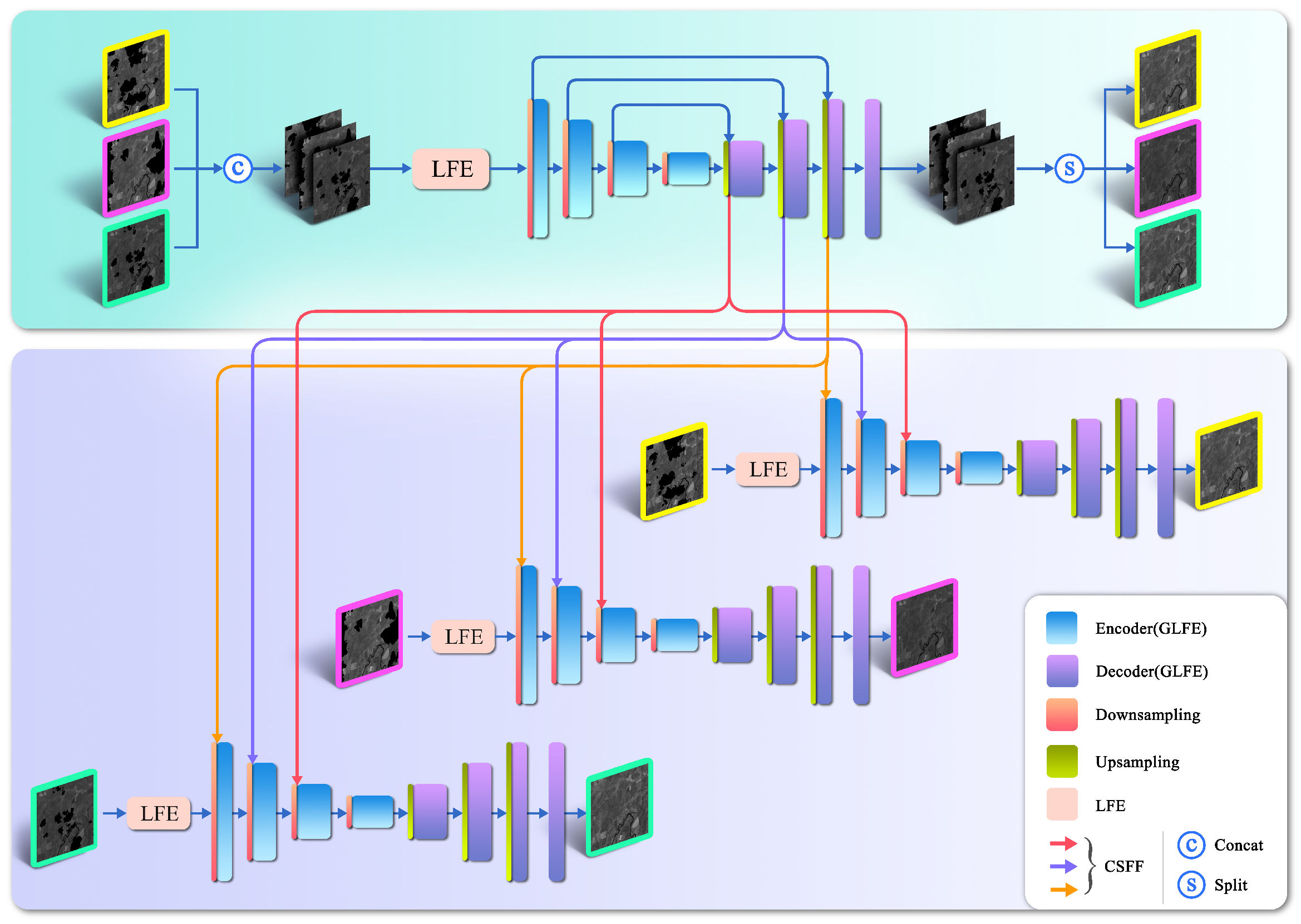
The overall framework of GLTF-Net is the TGL structure, which consists of two stages: the GMFF stage and the LSIR stage, as shown in the upper and lower parts of Figure 1. Each stage is composed of the feature global–local structure, which is a Transformer–CNN structure, combining the local feature extraction ability of CNN and the global feature fusion ability of Transformer. When restoring information in thick cloud occlusion regions, it ensures that multi-temporal information is fully utilized and the fine-grained information of the image is retained to a great extent. The two stages are detailed in

Table 2. Details of the GMFF and LSIR structures, where G represents the number of input phases, C represents the input channel, and H and W represent the height and width of the image, respectively.

Modules	Layer	Input	Output
LFE	Conv3 × 3	GC × H × W	GC1 × H × W
	Conv3 × 3	GC1 × H × W	GC1 × H × W
	Conv3 × 3	GC1 × H × W	C1 × H × W
	Conv1 × 1	GC × H × W	C1 × H × W
Encoder1	Conv3 × 3	C1 × H × W	GC1 × H × W
	Normalization	GC1 × H × W	GC1 × H × W
	Conv3 × 3	GC1 × H × W	C1 × H × W
	Transformer	C1 × H × W	C1 × H × W
⋮	⋮	⋮	⋮
Mid	Conv4 × 4	4C1 × H/4 × W/4	8C1 × H/8 × W/8
	Conv3 × 3	8C1 × H/8 × W/8	8GC1 × H/8 × W/8
	Normalization	8GC1 × H/8 × W/8	8GC1 × H/8 × W/8
	Conv3 × 3	8GC1 × H/8 × W/8	8C1 × H/8 × W/8
	Transformer	8C1 × H/8 × W/8	8C1 × H/8 × W/8
⋮	⋮	⋮	⋮
Decoder3	Conv2 × 2	2C1 × H/2 × W/2	C1 × H × W
	Conv3 × 3	C1 × H × W	GC1 × H × W
	Normalization	GC1 × H × W	GC1 × H × W
	Conv3 × 3	GC1 × H × W	C1 × H × W
	Transformer	C1 × H × W	C1 × H × W
Refinement	Conv3 × 3	C1 × H × W	GC1 × H × W
	Normalization	GC1 × H × W	GC1 × H × W
	Conv3 × 3	GC1 × H × W	C1 × H × W
	Transformer	C1 × H × W	C1 × H × W
OutLayer	Conv3 × 3	C1 × H × W	GC × H × W

.

(1) Global multi-temporal feature fusion stage: This stage focuses on the global multi-temporal feature fusion; therefore, the input at this stage is a cascade image $\widehat{X}$ of three temporal images $X^1$, $X^2$ and $X^3$ in the channel dimension. The LFE module performs local feature extraction for the multi-temporal feature map and the single-temporal feature map in two stages, retaining the fine-grained information in the original image, and then the encoding-decoding structure composed of the GLFE module fuses and extracts features on the multi-scale feature map by upsampling and downsampling. In the Transformer–CNN structure of the GLFE module, the Transformer structure integrates the global multi-temporal feature in the channel dimension, while the CNN structure retains the local fine-grained information during the feature fusion process, and prevents the edge and texture details in the single-temporal images during the multi-temporal fusion. At the end of the GMFF stage, the feature map is separated, and $\widehat{X^1}$, $\widehat{X^2}$ and $\widehat{X^3}$ are the output of this stage. The structure is as follows:

$$\widehat{X}=Concat(X^1,X^2,X^3)$$

(1)

$$\widehat{X_1}=\mathcal{R}(\mathcal{S}\left(\widehat{X}\right)+\widehat{X})+\widehat{X}$$

(2)

$$\widehat{X_1^1},\widehat{X_1^2},\widehat{X_1^3}=Split\left(\widehat{X_1}\right)$$

(3)

where $\mathcal{S}(·)$ represents the LFE module, $\mathcal{R}(·)$ represents the GLFE module, and $Concat(·)$ and $Split(·)$ represent the concatenation and separation of features, respectively.

(2) Local single-temporal information restoration stage: This stage focuses on local single-temporal information restoration. Although the network for each temporal image is roughly similar to the GMFF stage, there are specific differences in module details that better align with the global–local characteristics. In the LSIR stage, the individual temporal image $X^k$ is input, respectively. The outputs of each layer of the GMFF stage are combined to obtain fusion features at different scales. These fusion features are integrated into this stage as auxiliary information to promote the single-temporal information restoration and achieve accurate and comprehensive thick cloud removal. The structure is as follows:

$$\widehat{X_2^k}=\mathcal{R}\left(Concat(\mathcal{S}\left(X^k\right)+X^k,X^{\mathcal{R}})\right)+X^k,k\in \{1,2,3\}$$

(4)

where $\widehat{X_2^k}$ represents the output corresponding to the $k_{th}$ temporal image in the LSIR stage, while $X^R$ represents the fusion feature information that the GLFE module transmits across phases in the GMFF stage.

3.2. Local Feature Extraction Module

In the task of multi-temporal thick cloud removal, detailed information is important for the restoration of thick cloud occlusion information. Although the Transformer network performs well in global feature extraction, we believe that CNN is more effective in local feature extraction and can provide stable optimization for subsequent deep feature fusion and extraction. The LFE module, which is a CNN component within the Transformer–CNN structure, is located at the front of each stage network. By doing so, it can focus more on the local feature extraction in the feature global–local structure. It is worth noting that the LFE module intentionally avoids downsampling operations, ensuring that the spatial resolution of the feature maps remains consistent with the original image. Consequently, this module can concentrate on fine-grained feature extraction such as local textures, edges, etc.

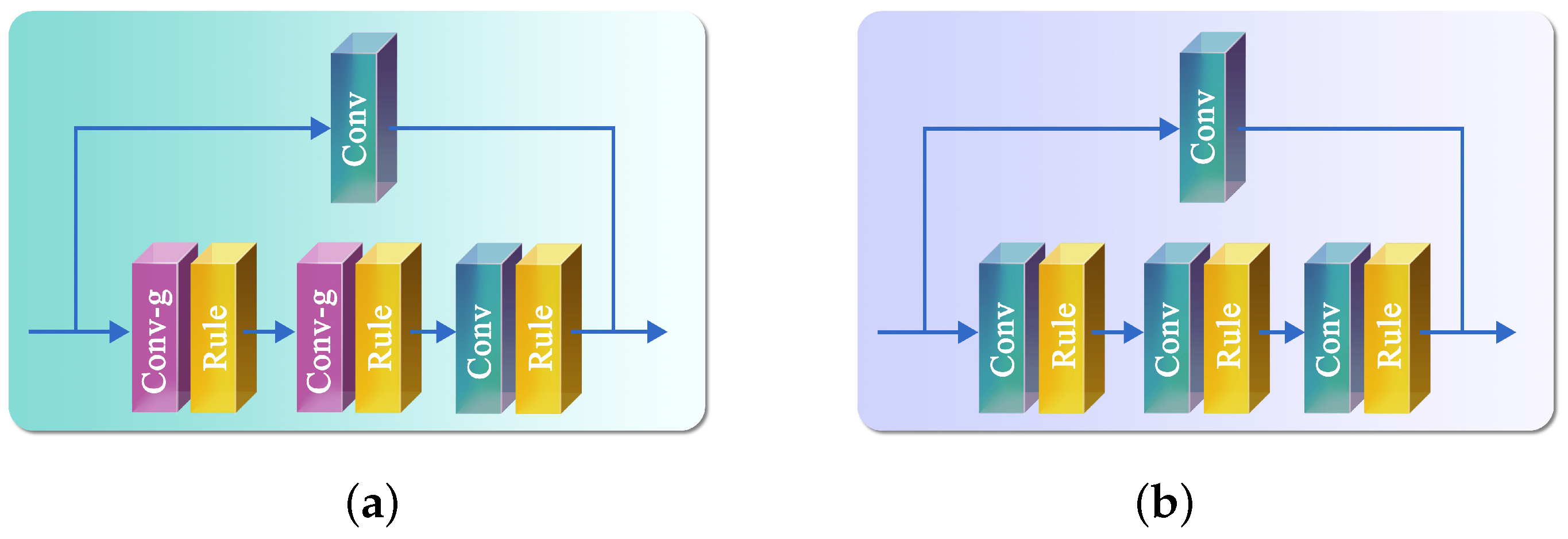
The LFE module consists of convolutional layers and ReLU non-linear activation functions. The initial two convolutions employ group convolution. In the GMFF stage, there are three groups corresponding to the concatenated input of three temporal images. This allows for the local feature extraction from each temporality at a local temporal level. Subsequently, after two ordinary convolutions and ReLU activation functions, the local features at the global temporality level in the cascaded image are extracted, as shown in the first part of Figure 2. In the LSIR stage, three single temporal images are inputted separately, and there is no need for group convolution, so the group parameter is set to 1, as shown in the second part of Figure 2. The embedding process of the LFE module is as follows:

$$X_g=Relu\left(Con{v}_g\left(Relu\left(Con{v}_g\left(X\right)\right)\right)\right)$$

(5)

$$\widehat{X_{\mathcal{S}}}=Conv\left(X\right)+Relu\left(Conv\left(Relu\left(Conv\left(X_g\right)\right)\right)\right)$$

(6)

where X represents the input image, $X_g$ and $\widehat{X_{\mathcal{S}}}$ represent the output feature map of the group convolution and the output of the LFE module, respectively, and $Conv(·)$, $Con{v}_g(·)$, and $Relu(·)$ represent the ordinary convolution, group convolution, and Relu activation function, respectively.

3.3. Global–Local Feature Extraction Module

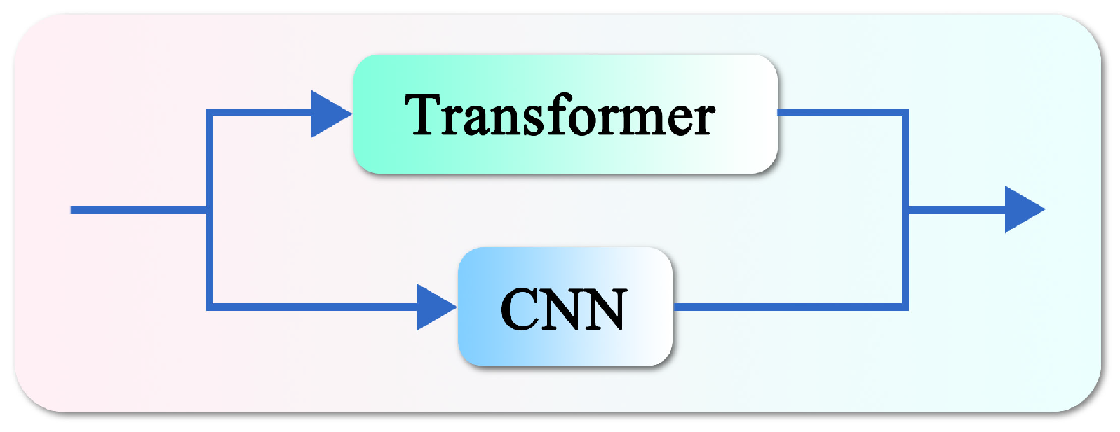
The GLFE module consists of a Transformer–CNN structure, as shown in Figure 3. The Transformer [26] introduced in this paper is different from the window attention-based Transformer [27,28] as described here. It implicitly encodes global context information by calculating attention on the channel, and the global feature can be extracted and fused from the input image in the channel dimension. Additionally, it employs a gate network to further filter out useful information. The structured process is as follows. In the task of multi-temporal thick cloud removal, it is particularly suitable for fusing long-distance dependent features of the global multi-temporal feature maps in feature global–local structure. By combining the information from cloud-free regions in different temporal images, it is able to restore the local single-temporal image missing ground information. However, because the Transformer focuses on capturing global information interaction, its ability to extract fine-grained details, such as local texture, is generally moderate. In the cloud removal task, the characteristics of fine-grained information such as edges and textures are crucial. Therefore, a CNN branch is added to the GLFE module to retain as much local detailed information as possible while fusing global channel features. The embedding process of the GLFE module is as follows:

$$\widehat{X_{\mathcal{G}}}=\widehat{X_{\mathcal{C}}}+\widehat{X_{\mathcal{T}}}$$

(7)

$$\widehat{X}=W_{p}Attention(\widehat{Q},\widehat{K},\widehat{V})+X$$

(8)

$$Attention(\widehat{Q},\widehat{K},\widehat{V})=\widehat{V}·Softmax(\widehat{K}·\widehat{Q}/\alpha )$$

(9)

$$\widehat{X_{\mathcal{T}}}=W_p^{0}Gating\left(\widehat{X}\right)+\widehat{X}$$

(10)

$$Gating\left(\widehat{X}\right)=\phi \left(W_d^1{W}_p^1\left(LN\left(X\right)\right)\right)\odot W_d^2{W}_p^2\left(LN\left(X\right)\right)$$

(11)

where $\widehat{X_{\mathcal{G}}}$, $\widehat{X_{\mathcal{C}}}$, and $\widehat{X_{\mathcal{T}}}$ represent the output of the GLFE module, Transformer branch and CNN branch, respectively. X and $\widehat{X}$ are the input and output feature maps. $\widehat{Q}$, $\widehat{V}\in R^{\widehat{H}\widehat{W}\times \widehat{C}}$, and $\widehat{K}\in R^{\widehat{C}\times \widehat{H}\widehat{W}}$ matrices are obtained after reshaping tensors from the original size $R^{\widehat{H}\times \widehat{W}\times \widehat{C}}$. Here, $\alpha$ is a learnable scaling parameter. $W_p^{(·)}$ is the 1 × 1 point-wise convolution and $W_d^{(·)}$ is the 3 × 3 depth-wise convolution. ⊙ denotes element-wise multiplication, $\phi$ represents the GELU non-linearity, and LN is the layer normalization.

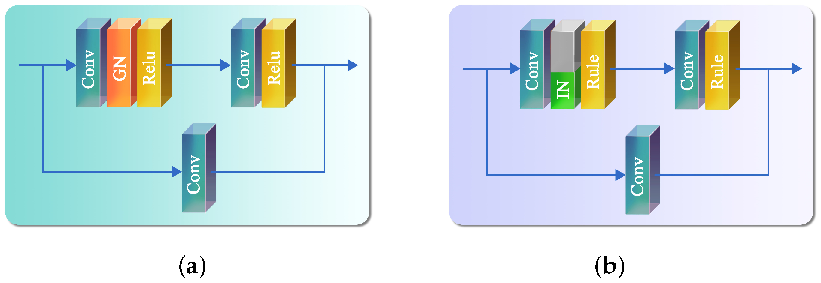
The CNN branch in the Transformer–CNN structure of the GLFE module is based on the half instance normalization block [29]. To better align with the feature global–local structure, we have made appropriate improvements to the half-instance normalization block. The difference between the GMFF stage and the LSIR stage lies in the normalization method: In the GMFF stage, group normalization is applied to the global multi-temporal feature map across all channels. Since the input in this stage is a concatenation of three temporal images, group normalization divides the feature map into three groups in the channel dimension. It calculates and normalizes the mean and variance of features at the local level, ensuring the accuracy of information interaction during feature fusion, as shown in the first part of Figure 4. In the LSIR stage, the local single-temporal feature map is divided into two parts in the channel dimension. The first half is instance-normalized and then concatenated with the second half in the channel dimension to restore the original size of the feature map, as shown in the second part of Figure 4. Additionally, to further balance the weights of residual connections and improve the feature extraction ability of the structure, the learnable parameters to both branches have been added, as shown in Equation (10). The CNN embedding process in the Transformer–CNN structure of the GLFE module is as follows:

$$\widehat{X_{\mathcal{C}1}}=Relu\left(Conv\left(Relu\left(Norm\left(Conv\left(\widehat{X_{\mathcal{G}1}}\right)\right)\right)\right)\right)$$

(12)

$$\widehat{X_{\mathcal{C}2}}=Conv\left(\widehat{X_{\mathcal{G}1}}\right)$$

(13)

$$\widehat{X_{\mathcal{C}}}=\alpha \widehat{X_{\mathcal{C}1}}+(1-\alpha )\widehat{X_{\mathcal{C}2}}$$

(14)

where $\widehat{X_{\mathcal{C}1}}$, $\widehat{X_{\mathcal{C}2}}$, and $\widehat{X_{\mathcal{C}}}$ represent the outputs of the first convolution branch, the second convolution branch, and the combined output of the convolutional, respectively. $Norm(·)$ represents normalization.

3.4. Cross-Stage Information Transfer

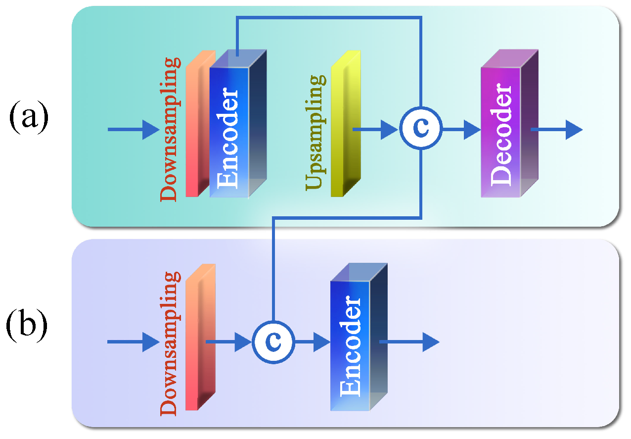
Referring to the idea of cross-stage feature fusion [30], a new cross-stage information transfer method is designed according to the temporality global–local structure. In the GMFF stage, the features of cloud-free regions between multi-temporal are integrated. As auxiliary information, these fusion features are transmitted to the LSIR stage across stages and promote the restoration of thick cloud occlusion information. The specific structure is shown in Figure 5.

In the GMFF stage, the skip connection of the encoder is cascaded with the output of upsampling. It is passed to the decoder first and then passed to the LSIR stage, where it is combined with the output of the downsampling concatenate before being transmitted to the encoder. It is worth noting that cross-stage information transfer operations are performed in each GLFE module to ensure the integrity of information at different scales, thereby helping to restore the information in the LSIR stage.

3.5. Loss Function Design

A temporality global–local loss function based on the temporality global–local structure is proposed. Specifically, the loss function is calculated separately in the GMFF stage and the LSIR stage. In the GMFF stage, considering that the local differences among multi-temporal images can affect the restoration of thick cloud occlusion information with global consistency, the loss function is calculated. The goal is to eliminate the imbalance between global invariance and local variations. In the LSIR stage, the loss function is calculated to ensure the accuracy of restoring the local single-temporal image thick cloud occlusion information, aiming to make the restored image closer to the real cloud-free image. The expression of the temporality global–local loss function $Loss$ is as follows:

$$Loss={\lambda }_{1}Los{s}_1+{\lambda }_{2}Los{s}_2$$

(15)

where $Los{s}_1$ and $Los{s}_2$ represent the loss function in the GMFF stage and LSIR stage loss function, respectively, and ${\lambda }_1$ and ${\lambda }_2$ are the weight parameters for balancing the loss of the two stages.

Considering the global–local feature, the loss function in each stage is divided into two parts: In the first part, the overall difference between the restored thick cloud image and the real cloud-free image can be measured by calculating their L1 distance, aiming to maintain global consistency. In the second part, the loss function focuses on the detailed information occluded by the thick cloud, ensuring the local detail consistency between the restored thick cloud image and the real cloud-free image. The expression of the loss function is as follows:

$$\begin{array}{cc}\hfill Los{s}_{1,2}=& \sum _{k=1}^3\left(\frac{1}{N}\sum _{i=1}^N(I_i^k-\widehat{I_i^k})\right)+\sum _{k=1}^3(\frac{1}{N_{repair}}\sum _{i=1}^{N_{repair}}(I_i^k-\widehat{I_i^k})\hfill \\ & +{\lambda }_3\frac{1}{N_{non-repair}}\sum _{i=1}^{N_{non-repair}}(I_i^k-\widehat{I_i^k}))\hfill \end{array}$$

(16)

where N, $N_{repair}$, and $N_{non-repair}$ represent the total number of image pixels, the number of pixels blocked by thick cloud and the number of pixels not blocked, respectively, $I_k$ and $\widehat{I_k}$ represent the generated image of the $k_{th}$-temporal image and the real cloud-free image, and ${\lambda }_3$ is used to balance the global and local relations.

4. Experiment

On various data sets, we ran comparative experiments to verify the performance of the proposed GLTF-Net. In this section, we first describe the data sets and the comparative methods used, then introduce the environment and parameter settings for model training. Finally, we compared the proposed method to four comparative methods in different scenes, presented the quantitative and qualitative experimental results, and analyzed the experimental results.

4.1. Data Set and Comparative Methods

As seen in

Table 3. Data set descriptions.

Region	Data	Number	Scene	Size	Band
Canberra	21 November 2021	2400 (200 × 4 × 3)	Farmland River	$256\times 256$	B2 (Blue) B3 (Green) B4 (Red) B5 (NIR)
	3 December 2021
	21 December 2021
Wuhan	12 May 2013	2988 (996 × 4 × 3)	Town Road
	13 June 2013
	31 July 2013
Tongchuan	22 November 2021	576 (48 × 4 × 3)	Mountain
	1 January 2022
	9 January 2022

, a total of 5964 remote sensing images with a size of $256\times 256$ pixels made up the synthetic data set used in this paper. Four spectral bands of Landsat8—B2 (blue), B3 (green), B4 (red), and B5 (NIR)– are present for each temporality in each of the three temporal images that make up each image. The synthetic data set consists of four scenes that were acquired in Canberra, Tongchuan, and Wuhan. The four scenes represent farmland, mountain, river, and town road, respectively.

We employed the Landsat 8 OLI/OLI-TIRS Level-1 Quality Assessment (QA) 16-bit bands to produce synthetic cloud masks, where pixels that visually resemble clouds are labeled as clouds, resulting in synthetic cloud masks. For the first, second, and third temporal images, the cloud occlusion percentages are kept at 20% to 30%, 10% to 20%, and 5% to 15%, respectively.

We tested four scenes, each with 36 images of size $256\times 256$, in the test data set to assess the restoration precision by the proposed GLTF-Net on different scene data sets. To confirm the effectiveness of the proposed method on test data in the real world, we also use the Sentinel-2 real data set. This data set has a spatial resolution of 20 m and consists of the spectral bands B5, B7, and B11. The test images comprise a total of 9 images with the size of 3000 × 3000.

Both the training and test data sets in this paper are sourced from the United States Geological Survey (USGS) (https://www.usgs.gov/).

The comparative methods chosen in this section are WLR, STS, PSTCR [31], and CMSN. Among these, the WLR is a classical method for multi-temporal cloud removal and can directly accept the missing image and supplemental images from the other temporality as input and does not require training and learning. The official version of WLR used in this section is 2016.11.3_2.0. STS and PSTCR are two commonly used deep learning methods, while CMSN is currently the best-performing method for multi-temporal cloud removal in deep learning. Therefore, these four methods were selected for comparative experiments. The comparative results are shown in Figure 6.

4.2. Implementation Details

The system and software environments in this experiment are Ubuntu 20.04 and Pytorch 1.11.0+cu113, respectively. The NVIDIA TESLA V100 GPU and NVIDIA RTX A5000 GPU are used for training and testing, respectively, for the methods based on deep learning.

During training, the Adam optimizer is used to optimize the model’s parameters with an initial learning rate set to 0.0003. Every 20 epochs, the learning rate is decreased by a factor of 0.8. There are 200 training epochs in total. The batch size is set to 3. The values of ${\lambda }_1$, ${\lambda }_2$ and ${\lambda }_3$ are 0.3, 0.7 and 0.15, respectively. All deep learning methods compared in this section are trained using the same training data set and on the same hardware and software platforms to ensure fairness.

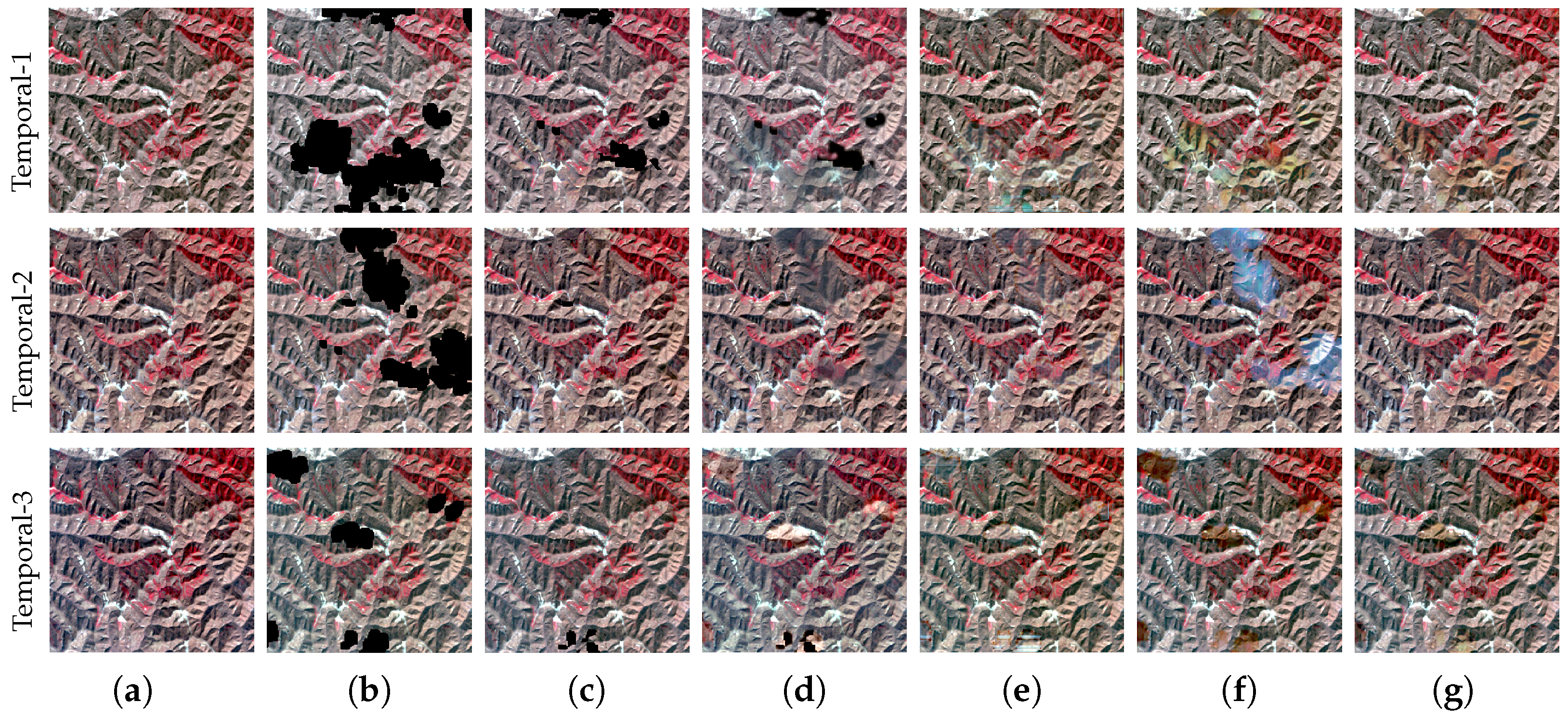
First, the restoration performances by various methods are evaluated quantitatively using four widely used indexes: PSNR, SSIM (structural similarity), CC, and RMSE (root mean square error). The average quantitative results are shown in

Table 4. The average quantitative evaluation indexes of the four testing images in different scenarios. The average values of four bands, including B2, B3, B4, and NIR, are considered. Red indicates the best performance and blue indicates the second best.

Index	Temporal	WLR	STS	PSTCR	CMSN	GLTF
PSNR	Temporal-1	37.1015	36.5240	39.5575	42.7643	45.4393
	Temporal-2	38.7784	35.5123	41.0762	42.4402	47.6657
	Temporal-3	40.4874	39.5753	44.5759	48.2452	53.2275
	Average	38.7891	37.2039	41.7365	44.4832	48.7775
SSIM	Temporal-1	0.9563	0.9698	0.9829	0.9929	0.9951
	Temporal-2	0.9693	0.9698	0.9873	0.9910	0.9970
	Temporal-3	0.9611	0.9758	0.9920	0.9971	0.9986
	Average	0.9622	0.9718	0.9874	0.9936	0.9969
CC	Temporal-1	0.8709	0.8716	0.9279	0.9651	0.9811
	Temporal-2	0.9048	0.8952	0.9544	0.9193	0.9851
	Temporal-3	0.8637	0.8778	0.9545	0.9787	0.9932
	Average	0.8798	0.8815	0.9456	0.9544	0.9864
RMSE	Temporal-1	0.0183	0.0180	0.0125	0.0079	0.0061
	Temporal-2	0.0120	0.0169	0.0096	0.0089	0.0050
	Temporal-3	0.0149	0.0142	0.0073	0.0043	0.0028
	Average	0.0151	0.0164	0.0098	0.0070	0.0046

. The quantitative results for the various methods in different scenarios are shown in

Table 5. Quantitative evaluation indexes for simulated experiments in farmland scenes. The value of each temporal image is displayed in the format of Temporal-1/Temporal-2/Temporal-3. Red indicates the best performance and blue indicates the second best.

Index	Band	WLR	STS	PSTCR	CMSN	Ours
PSNR	B2	44.1876/38.4585/44.6980	41.7397/37.4393/44.4925	45.0408/45.4720/47.5060	47.8481/39.2984/50.3178	52.8676/51.7432/54.9451
	B3	41.6750/36.1619/42.1653	40.9196/35.2803/41.7105	42.5667/43.2027/45.8016	45.6621/43.3613/47.8202	51.0967/51.6316/54.4066
	B4	39.4027/34.8883/39.7899	38.8772/33.9929/39.6632	41.0923/41.4258/44.4575	43.5455/43.4757/45.6413	47.6637/49.3275/51.0192
	NIR	30.7066/26.8822/31.5439	30.8134/26.6185/31.3726	33.5616/41.4257/35.7688	41.7619/45.1603/45.1902	42.4717/46.1059/46.1152
SSIM	B2	0.9680/0.9639/0/9685	0.9791/0.9674/0.9820	0.9929/0.9925/0.9956	0.9968/0.9856/0.9975	0.9988/0.9986/0.9992
	B3	0.9617/0.9607/0.9640	0.9785/0.9649/0.9786	0.9907/0.9901/0.9944	0.9965/0.9941/0.9974	0.9986/0.9987/0.9992
	B4	0.9577/0.9593/0.9599	0.9755/0.9630/0.9762	0.9880/0.9873/0.9931	0.9950/0.9939/0.9964	0.9972/0.9978/0.9985
	NIR	0.9379/0.9473/0.9467	0.9572/0.9447/0.9585	0.9682/0.9731/0.9807	0.9935/0.9961/0.9963	0.9936/0.9963/0.9967
CC	B2	0.8653/0.7948/0.8780	0.8064/0.7709/0.8893	0.8922/0.9731/0.9413	0.9410/0.7822/0.9642	0.9795/0.9858/0.9886
	B3	0.8674/0.8349/0.8900	0.8673/0.8159/0.8978	0.9225/0.9525/0.9618	0.9615/0.9482/0.9752	0.9882/0.9939/0.9944
	B4	0.9147/0.8953/0.9269	0.9201/0.8829/0.9305	0.9535/0.9712/0.9772	0.9729/0.9815/0.9825	0.9889/0.9959/0.9944
	NIR	0.7747/0.7127/0.7356	0.7839/0.7047/0.7551	0.8719/0.8935/0.8903	0.9856/0.9909/0.9872	0.9871/0.9916/0.9893
RMSE	B2	0.0073/0.1213/0.0066	0.0086/0.0138/0.0063	0.0056/0.0058/0.0042	0.0041/0.0114/0.0031	0.0023/0.0084/0.0018
	B3	0.0106/0.0159/0.0090	0.0103/0.0177/0.0087	0.0076/0.0076/0.0052	0.0053/0.0072/0.0041	0.0028/0.0027/0.0019
	B4	0.0134/0/0183/0.0110	0.0129/0.0208/0.0107	0.0091/0.0093/0.0061	0.0068/0.0071/0.0053	0.0042/0.0035/0.0029
	NIR	0.0373/0.0456/0.0331	0.0339/0.0474/0.0312	0.0242/0.0227/0.0185	0.0082/0.0062/0.0060	0.0077/0.0057/0.0054

,

Table 6. Quantitative evaluation indexes for simulated experiments in town road scenes. The value of each temporal image is displayed in the format of Temporal-1/Temporal-2/Temporal-3. Red indicates the best performance and blue indicates the second best.

Index	Band	WLR	STS	PSTCR	CMSN	Ours
PSNR	B2	38.7173/37.0642/38.6127	38.2585/36.4365/39.6303	41.1198/41.7825/44.5351	43.2101/43.0855/48.8004	46.0383/50.0596/52.1968
	B3	35.5017/34.5651/35.7913	36.1655/34.1450/37.0481	38.8712/39.4097/41.8833	41.8974/46.4160/45.1040	44.4856/48.7407/50.0584
	B4	33.0758/32.3934/33.4166	33.9309/32.1194/34.4064	36.9622/36.7149/39.0813	40.0231/42.9447/42.6631	41.6520/45.2349/46.2871
	NIR	26.2572/26.2499/26.3383	27.4102/26.4647/27.7358	29.5522/30.8273/34.4811	36.6979/40.6828/42.3910	37.1817/40.6343/43.2253
SSIM	B2	0.9568/0.9524/0.9465	0.9726/0.9672/0.9715	0.9879/0.9906/0.9919	0.9932/0.9933/0.9972	0.9962/0.9982/0.9985
	B3	0.9482/0.9454/0.9371	0.9726/0.9637/0.9674	0.9847/0.9874/0.9893	0.9934/0.9940/0.9955	0.9955/0.9978/0.9980
	B4	0.9368/0.9418/0.9277	0.9646/0.9588/0.9590	0.9790/0.9811/0.9838	0.9902/0.9939/0.9934	0.9920/0.9956/0.9959
	NIR	0.9198/0.9275/0.9116	0.9459/0.9401/0.9418	0.9516/0.9643/0.9726	0.9853/0.9920/0.9941	0.9857/0.9914/0.9946
CC	B2	0.8664/0.8500/0.8359	0.8464/0.9400/0.8619	0.9118/0.9439/0.9384	0.9432/0.9484/0.9751	0.9710/0.9908/0.9877
	B3	0.8296/0.8291/0.8130	0.8393/0.8338/0.8460	0.9022/0.9362/0.9285	0.9502/0.9482/0.9618	0.9716/0.9917/0.9870
	B4	0.8426/0.8670/0.8425	0.8623/0.8682/0.8667	0.9210/0.9440/0.9435	0.9613/0.9814/0.9728	0.9730/0.9914/0.9877
	NIR	0.7955/0.8301/0.7412	0.8355/0.8427/0.7886	0.8868/0.9304/0.9416	0.9729/0.9904/0.9901	0.9752/0.9905/0.9946
RMSE	B2	0.0117/0.0143/0.0118	0.0122/0.0152/0.0105	0.0088/0.0081/0.0061	0.0071/0.0075/0.0038	0.0050/0.0032/0.0026
	B3	0.0169/0.0192/0.0164	0.0155/0.0198/0.0141	0.0114/0.0107/0.0083	0.0083/0.0072/0.0059	0.0059/0.0038/0.0034
	B4	0.0223/0.0245/0.0214	0.0201/0.0250/0.0190	0.0141/0.0147/0.0115	0.0100/0.0071/0.0080	0.0082/0.0056/0.0052
	NIR	0.0489/0.0607/0.0488	0.0427/0.0491/0.0414	0.0334/0.0287/0.0197	0.0146/0.0100/0.0079	0.0139/0.0100/0.0073

,

Table 7. Quantitative evaluation indexes for simulated experiments in river scenes. The value of each temporal image is displayed in the format of Temporal-1/Temporal-2/Temporal-3. Red indicates the best performance and blue indicates the second best.

Index	Band	WLR	STS	PSTCR	CMSN	Ours
PSNR	B2	42.1776/47.4429/45.0453	42.4433/39.3398/45.1556	44.5265/45.9298/49.5491	47.3045/41.1645/54.5883	50.4506/52.3916/59.2241
	B3	39.2449/45.2949/41.9808	40.6094/37.2447/42.1135	42.3560/43.8700/48.7175	45.5671/45.3435/50.7487	48.7172/50.6990/57.7561
	B4	36.7982/42.7598/39.9649	38.0949/35.9445/40.0553	39.4058/41.5597/47.0276	41.7003/44.4141/48.7017	44.1523/47.5465/54.6828
	NIR	29.9649/36.8284/31.0532	30.0344/29.0705/31.1859	31.9493/34.9691/40.3278	38.3284/43.6823/48.8393	39.3180/43.5832/47.0305
SSIM	B2	0.9744/0.9938/0.9740	0.9881/0.9830/0.9863	0.9925/0.9957/0.9971	0.9961/0.9919/0.9990	0.9980/0.9990/0.9996
	B3	0.9669/0.9919/0.9689	0.9878/0.9827/0.9833	0.9910/0.9942/0.9972	0.9960/0.9960/0.9982	0.9979/0.9986/0.9996
	B4	0.9568/0.9888/0.9657	0.9822/0.9804/0.9803	0.9846/0.9911/0.9972	0.9919/0.9955/0.9976	0.9943/0.9976/0.9991
	NIR	0.9452/0.9864/0.9504	0.9632/0.9672/0.9611	0.9648/0.9802/0.9905	0.9901/0.9964/0.9982	0.9907/0.9964/0.9982
CC	B2	0.9231/0.9638/0.8471	0.8718/0.8156/0.8729	0.9167/0.9486/0.9566	0.9578/0.8700/0.9861	0.9906/0.9865/0.9952
	B3	0.9094/0.9694/0.8510	0.8960/0.8450/0.8743	0.9308/0.9560/0.9744	0.9578/0.9709/0.9830	0.9844/0.9902/0.9968
	B4	0.9240/0.9789/0.8972	0.9241/0.9103/0.9102	0.9423/0.9704/0.9848	0.9669/0.9857/0.9889	0.9812/0.9926/0.9972
	NIR	0.9199/0.9767/0.8257	0.9096/0.8948/0.8464	0.9378/0.9616/0.9818	0.9848/0.9949/0.9973	0.9880/0.9950/0.9961
RMSE	B2	0.0080/0.0043/0.0068	0.0076/0.0110/0.0061	0.0059/0.0051/0.0033	0.0043/0.0089/0.0019	0.0030/0.0024/0.0011
	B3	0.0112/0.0055/0.0096	0.0094/0.0140/0.0087	0.0076/0.0064/0.0036	0.0053/0.0054/0.0030	0.0037/0.0030/0.0013
	B4	0.0147/0.0073/0.0118	0.0126/0.0162/0.0110	0.0107/0.0084/0.0045	0.0083/0.0060/0.0038	0.0062/0.0042/0.0019
	NIR	0.0328/0.0149/0.0336	0.0317/0.0357/0.0307	0.0253/0.0187/0.0097	0.0123/0.0068/0.0037	0.0109/0.0068/0.0046

and

Table 8. Quantitative evaluation indexes for simulated experiments in mountain scenes. The value of each temporal image is displayed in the format of Temporal-1/Temporal-2/Temporal-3. Red indicates the best performance and blue indicates the second best.

Index	Band	WLR	STS	PSTCR	CMSN	Ours
PSNR	B2	42.9039/48.0421/51.6107	40.6483/46.0219/48.5294	44.6641/47.0648/49.7992	45.0606/37.1116/51.2637	46.1398/48.4159/60.0855
	B3	42.4303/47.3274/51.1078	38.5194/43.5410/47.5681	43.2432/45.9790/49.4113	43.3928/39.5783/50.9519	45.4958/46.8025/59.9930
	B4	39.4292/45.5683/49.7189	36.5393/40.6250/45.4254	41.7083/44.4609/49.4113	41.5548/39.5783/50.2897	45.6151/45.8549/58.9068
	NIR	32.7085/40.5275/44.9591	29.3784/33.9126/37.1121	36.2990/39.7538/46.0796	40.6736/42.7263/48.6113	43.2822/43.8790/55.6783
SSIM	B2	0.9681/0.9895/0.9913	0.9757/0.9931/0.9944	0.9924/0.9952/0.9978	0.9932/0.9691/0.9982	0.9940/0.9971/0.9997
	B3	0.9667/0.9887/0.9912	0.9699/0.9895/0.9943	0.9905/0.9940/0.9976	0.9922/0.9799/0.9980	0.9934/0.9957/0.9997
	B4	0.9648/0.9875/0.9906	0.9647/0.9840/0.9943	0.9886/0.9925/0.9974	0.9900/0.9869/0.9980	0.9947/0.9953/0.9996
	NIR	0.9575/0.9837/0.9883	0.9396/0.9660/0.9840	0.9777/0.9864/0.9956	0.9930/0.9943/0.9979	0.9953/0.9955/0.9993
CC	B2	0.8947/0.9451/0.8775	0.8741/0.9331/0.8946	0.9443/0.9506/0.9263	0.9472/0.6611/0.9477	0.9595/0.9644/0.9898
	B3	0.9277/0.9653/0.9308	0.9017/0.9463/0.9353	0.9645/0.9693/0.9586	0.9666/0.8495/0.9701	0.9763/0.9742/0.9952
	B4	0.9406/0.9735/0.9558	0.9159/0.9493/0.9504	0.9734/0.9783/0.9772	0.9703/0.9429/0.9832	0.9885/0.9841/0.9973
	NIR	0.9269/0.9777/0.9696	0.8904/0.9393/0.9247	0.9740/0.9821/0.9888	0.9906/0.9913/0.9938	0.9950/0.9934/0.9987
RMSE	B2	0.0076/0.0042/0.0035	0.0092/0.0053/0.0039	0.0058/0.0044/0.0032	0.0055/0.0145/0.0027	0.0050/0.0039/0.0010
	B3	0.0090/0.0047/0.0036	0.0118/0.0070/0.0043	0.0068/0.0051/0.0033	0.0071/0.0110/0.0028	0.0054/0.0047/0.0010
	B4	0.0113/0.0058/0.0043	0.0149/0.0097/0.0054	0.0082/0.0061/0.0036	0.0092/0.0094/0.0030	0.0053/0.0052/0.0011
	NIR	0.0251/0.0109/0.0076	0.0341/0.0205/0.0140	0.0153/0.0104/0.0051	0.0093/0.0073/0.0038	0.0069/0.0065/0.0017

, respectively. Each table involves the experimental results for the three temporal images and four spectral bands. Better restoration performance is typically indicated by higher PSNR, SSIM, and CC values as well as lower RMSE values. The restoration results of four scenes—farmland, mountain, river, and town road—are then compared as part of a qualitative evaluation. The first, second, and third rows in Figure 7, Figure 8, Figure 9 and Figure 10 correspond to the first, second, and third temporal images, respectively. We analyze factors like image clarity, detail preservation, and color distortion to assess how well various methods perform in different scenes. Finally, we plotted the scatter plots of the cloud-free images and the reconstructed images from the first temporal images for four different scenarios, as shown in Figure 11.

$$\begin{array}{c}\hfill \mathrm{MSE}=\frac{1}{n}\sum _{i=1}^n{(x-y)}^2\end{array}$$

(17)

where n represents the number of samples, x is the actual observed value, and y is the predicted value.

$$\begin{array}{c}\hfill \mathrm{PSNR}=10·{log}_{10}\left(\frac{L^2}{\mathrm{MSE}}\right)\end{array}$$

(18)

where L represents the maximum range of pixel values (for example, for an image, $L=255$ means a maximum of 255 per pixel).

$$\begin{array}{c}\hfill \mathrm{SSIM}(x,y)=\frac{(2{\mu }_x{\mu }_y+C_1)(2{\sigma }_{xy}+C_2)}{({\mu }_x^2+{\mu }_y^2+C_1)({\sigma }_x^2+{\sigma }_y^2+C_2)}\end{array}$$

(19)

where x and y represent the two images, respectively, $\mu$ represents the mean of the images, $\sigma$ represents the standard deviation of the images, ${\sigma }_{x}y$ represents the covariance of the two images, and $C1$ and $C2$ are constants.

$$\begin{array}{c}\hfill \mathrm{CC}(x,y)=\frac{{\sum }_{i=1}^n(x_i-\overline{x})(y_i-\overline{y})}{\sqrt{{\sum }_{i=1}^n{(x_i-\overline{x})}^2}\sqrt{{\sum }_{i=1}^n{(y_i-\overline{y})}^2}}\end{array}$$

(20)

where x and y represent the two images, respectively, $x_i$ and $y_i$ represent the pixels in them, respectively, n represents the number of elements in the dataset, and $\overline{x}$ and $\overline{y}$ represent the mean of x and y.

$$\begin{array}{c}\hfill \mathrm{RMSE}=\sqrt{\mathrm{MSE}}\end{array}$$

(21)

4.3. Experimental Results

On a synthetic data set of four scenes—farmland, mountain, river and town road—we thoroughly evaluate the proposed method and the comparative methods in this section.

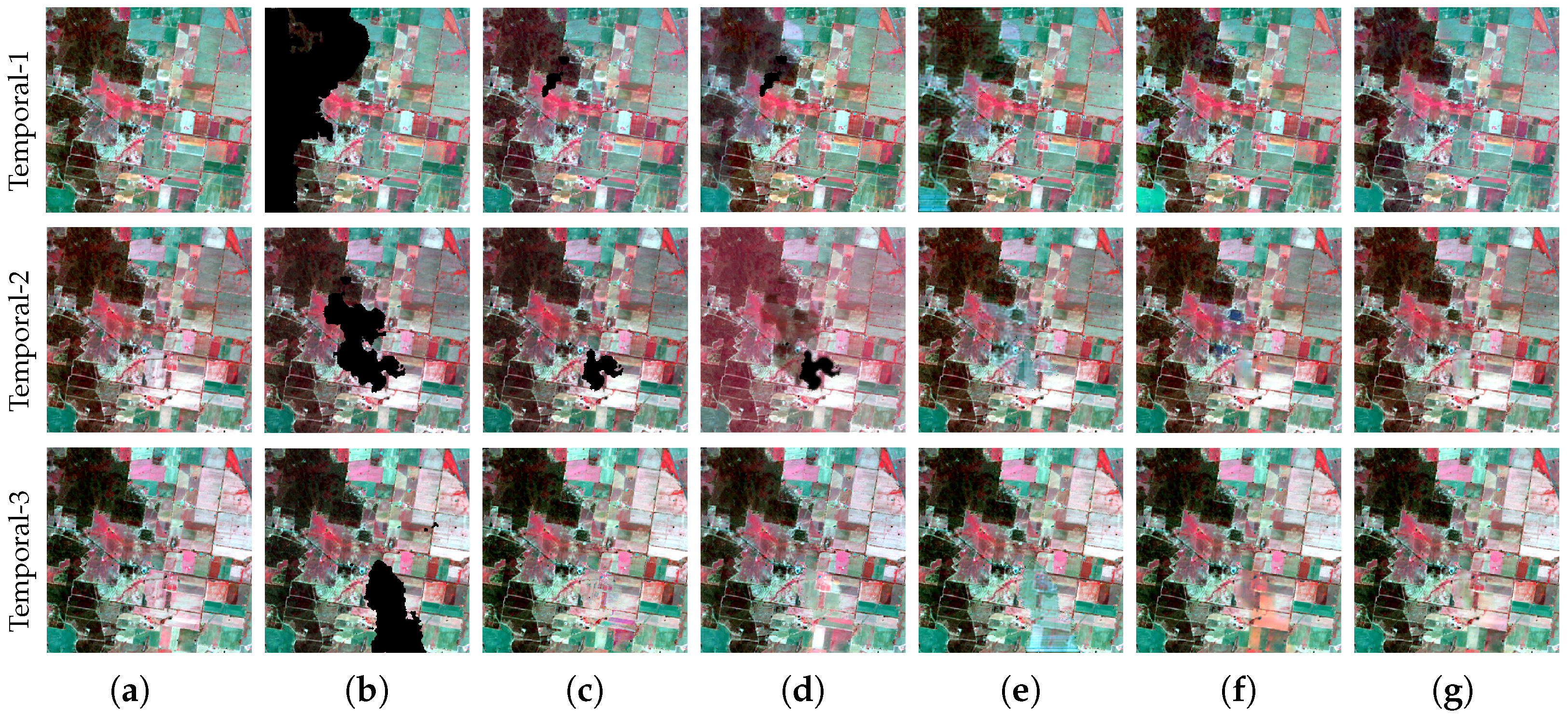
Farmland scenes: Figure 7 and Table 5 display the effects of five methods on the three temporal images in the farmland scenes when the thick cloud is removed. The figure shows that the WLR and STS methods have a limited ability to restore from overlapping cloud occlusion, leading to a significant amount of residual cloud and an incomplete restoration of ground information. In the qualitative experiments, the synthesized images are pseudo-colored images, and their colors are for reference purposes only. The PSTCR method shows obvious color distortion and has a poor ability to restore detailed information. In comparison, the results of the qualitative experiments show a significant improvement for both the CMSN and GLTF-Net. We find that the GLTF-Net performs better in restoring complex details when compared to the CMSN method. In the first temporal restored image’s lower left corner and left edge, as well as more noise in the dark region, the CMSN method exhibits observable color distortion. The GLTF-Net method’s overall restoration result is more realistic and similar to the original image, with better restoration of specific details.

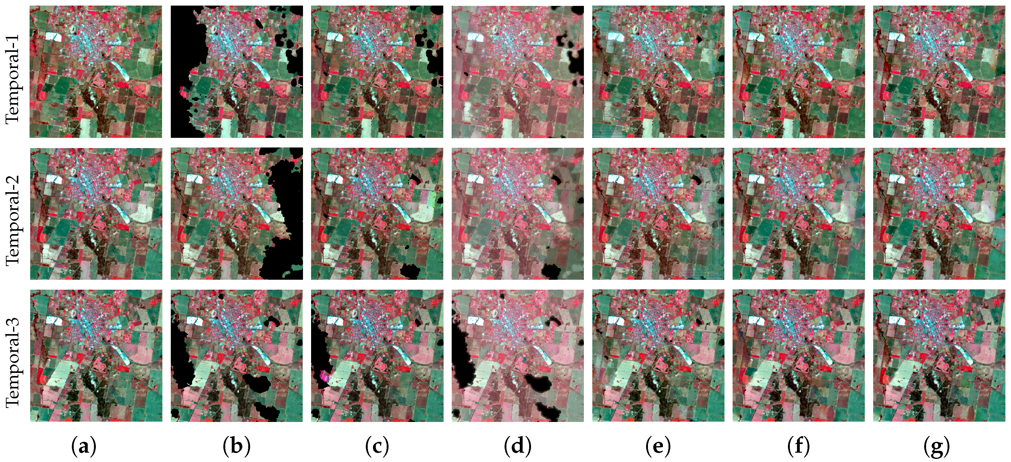
Town road scenes: Figure 8 and Table 6 demonstrate the effect of removing thick clouds from these scenes. The WLR, STS, and PSTCR methods exhibit limited ability of thick cloud removal, similar to agricultural field scenes. They result in noticeable color distortions in cloud occlusion regions and fall short of entirely removing residual clouds within the continuous range. The proposed GLTF-Net and the CMSN show better visual results. It is essential to note that the other two temporal images have a significant impact on the CMSN method, particularly in the first temporal image. The information interaction between the three temporal images has a minimal impact on the restoration results when the differences between each temporal image are small. However, there may be substantial differences in certain regions between the three temporal images that have a negative effect on the restoration’s quality. For instance, the first temporal image’s bottom left corner clearly exhibits color distortion, and the second temporal image’s middle-right region has an identical issue. In contrast, the proposed method outperforms the CMSN method and is less prone to the influence of temporal image inconsistencies, producing restoration outputs that closely resemble the original, cloud-free image.

River scenes: Figure 9 and Table 7 show the thick cloud removal effect in the river scenes. To accurately restore the river edge, a high level of detail restoration ability is required. If not, the river edge might be blurred, which can bring about an unnatural visual texture and loss of small details. Based on the qualitative findings, the bottom left corner of the second temporal images of all four comparative methods exhibit blurred river edge and color distortion. In order to precisely restore the river edge, a thick cloud restoration method with excellent detail restoration ability is essential. In this scene, the proposed GLTF-Net exhibits a superior ability to restore detailed features, leading to a more thorough restoration of the river edge. The near-infrared band of the third temporal image has a slightly weaker ability for information restoration, according to the quantitative experimental results.

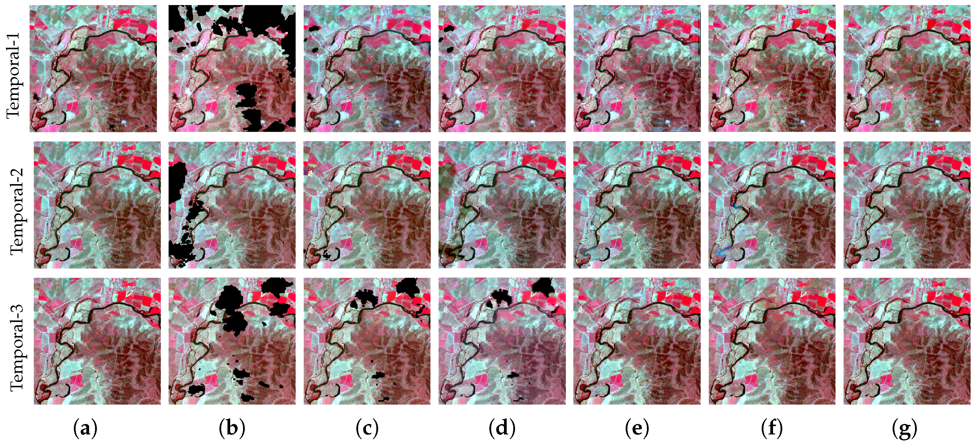
Mountain scenes: Figure 10 and Table 8 show the cloud removal results in a scene with mountains. Because of how uniform the colors are in mountainous settings, color distortion can have a big effect. Mountainous regions contain a lot of details, which pose challenges in fully restoring all the details. The four comparative methods are outperformed by the proposed GLTF-Net in both qualitative and quantitative experimental results. In the first and second temporal images, respectively, WLR and STS methods have issues with incomplete restoration, while PSNR and CMSN methods have issues with feature loss and color distortion. Quantitative experiments further show that the CMSN method performs poorly in restoring the second temporal image for the mountain scenes. Significant improvements have been made in addressing color distortion challenges by the planned GLTF-Net.

Real image: Figure 12 illustrates the cloud removal result in a scene with actual cloud occlusion. The first temporal image is more indicative of the cloud removal effect because it has more cloud occlusion. There are some overlaps of thick cloud occlusion in the second and third temporal images, and it is possible to observe how different cloud removal methods affect these overlaps. While the CMSN and STS methods show color distortion in the first temporal image, the WLR method encounters difficulties in eliminating the thick cloud occlusion. The PSTCR method performs well in color restoration suppression, but it introduces noticeable grid-like patterns in the restored regions, making ground details difficult to observe. It is clear from the second and third temporal images that the STS method falls short of fully restoring the ground information in the cloud occlusion regions where there is overlap. The PSTCR method yields poor restoration results with observable texture information loss. In the CMSN method, inter-temporal differences in the second temporal image’s lower right corner cause the brown region to be restored as green. The proposed GLTF-Net outperforms the previously mentioned methods in terms of both color restoration and detail restoration.

5. Discussion

The LFE and GLFE modules serve as the network’s fundamental blocks, and in this section, we conduct the ablation experiments on the established data set to evaluate how well the two modules work.

5.1. Effectiveness of LFE Module

To evaluate the effectiveness and necessity of the LFE module, a regular convolution is utilized in the GLTF-Net in place of the LFE module, the training is conducted while all other parameters are held constant, and the resulting model is tested on 900 images of the Canberra region test set, as depicted in Figure 13. The quantitative indexes of the ablation experiments are displayed in

Table 9. Quantitative evaluation of ablation experiment.

	PSNR	SSIM	CC	RMSE
GLTF without LFE	43.4894/48.9489/49.9420	0.9927/0.9976/0.9978	0.9609/0.9906/0.9868	0.0078/0.0042/0.0038
GLTF without GLFE-Trans	37.9671/41.4924/43.2449	0.9777/0.9892/0.9916	0.8718/0.9512/0.9453	0.0148/0.0100/0.0080
GLTF without GLFE-CNN	43.4334/48.5977/49.7107	0.9927/0.9975/0.9978	0.9605/0.9888/0.9860	0.0078/0.0044/0.0039
GLTF	43.8429/49.2274/50.1430	0.9932/0.9978/0.9979	0.9636/0.9908/0.9874	0.0075/0.0041/0.0037

. The terms GLTF without LFE and GLTF with LFE refer to the model with and without the LFE module, respectively. The PSNR, SSIM, and CC are improved by an average of 0.59%, 0.03%, and 0.12% for the average of three temporal images across the four bands, respectively, while the RMSE is reduced by 3.27%. In qualitative experiments, it is easier to see the color distortion between the upper left and upper right corners of GLTF without LFE. Quantitative experiments show that the LFE module may significantly improve the network’s ability to restore information during the cloud removal process and optimizes the subsequent feature fusion and extraction.

5.2. Effectiveness of GLFE Module’s Two Branches

The GLFE module includes a Transformer–CNN structure, in which we evaluate the effectiveness of the Transformer and the CNN branches, respectively, to more effectively extract global–local features. The qualitative assessment is shown in Figure 14.

First, we examine the effectiveness of the Transformer branch in the GLFE module. Table 9 displays the results of its ablation experiment. By introducing the Transformer branch in the GLFE module, under the average of four bands and three temporal images, there was an average increase of 16.71% in PSNR, 1.03% in SSIM, and 6.27% in CC. Additionally, there was an average reduction of 53.35% in RMSE. Without a Transformer branch, GLFE has a poor visual effect.

As shown in Table 9, the Transformer introduces the convolutional branch, thereby improving the GLFE module’s ability for missing information restoration. The GLFE module only uses the Transformer branch, not the convolutional branch, as indicated by GLTF without the GLFE-CNN branch. By introducing the Transformer branch in the GLFE module, under the average of four bands and three temporal images, there was an average increase of 0.1% in PSNR, 0.03% in SSIM, and 0.22% in CC. Additionally, there was an average reduction of 5.23% in RMSE. Without a CNN branch, GLFE faces the issue of an unnatural texture on the edge of a cloud occlusion region in terms of visual effects.

The results of the experiment indicate that the Transformer branch has a strong ability to capture global features and that the Transformer model can capture local information more effectively when combined with a convolution structure.

5.3. Limitations

Although the GLTF-Net proposed in this paper can remove the thick cloud more effectively, it has some disadvantages. First, even though the Transformer used in GLTF-Net is based on channel-based attention as opposed to window-based attention, it still has higher hardware requirements, which restricts study on thick cloud removal from a wider range of remote sensing images. Second, the synthetic data set used in this paper only includes the four bands of blue, green, red, and near-infrared, excluding other bands that have different reflectance and absorption properties. More band information may be beneficial in the restoration of thick cloud occlusion regions because different bands have different reflectance and absorption properties. However, this method is limited by the creation of the data set and the hardware conditions, as it only focuses on removing clouds from three temporalities in multi-temporal imagery. It does not attempt to remove clouds from a greater number of temporalities. Finally, the GLTF-Net can enhance the restoration ability of fine-grained information, but this improvement is only generalized to scenes with more complex detailed information. It is essential to further develop the method to increase the ability to restore fine-grained information. The future research direction is to develop lighter models specifically for Transformers. For example, this can be achieved by incorporating gating mechanisms to filter out unnecessary feature information that does not require computation or by modifying attention mechanisms to reduce computational costs. These advancements will enable the models to handle a wider range of spectral bands and effectively remove thick clouds in large-scale areas. Additionally, there will be attempts to extend the application of thick cloud removal to multi-modal data.

6. Conclusions

In this paper, we propose GLTF-Net, a network for remote sensing thick cloud removal that aggregates global–local temporalities and features. We first design the temporality global–local structure that distinguishes between multi-temporal inputs and single-temporal inputs, and then design the feature global–local structure and its LFE and GLFE modules combining Transformer’s global feature extraction with CNN’s local feature extraction in the GMFF stage and the LSIR stage.

In order to combine global temporal and spatial information and restore information from the local thick cloud occlusion region, single-temporal image self-correlation and multi-temporal image inter-correlation are used. In the GMFF stage, the cloud-free region features of each temporality are combined while retaining the detailed information. To make full use of the inter-correlation of the multi-temporal, the multiscale fusion information from the GMFF stage is added when restoring the thick cloud occlusion information in the local single-temporal information restoration stage. The temporality global–local sturcture’s processing method also fully considers the consistency and difference between temporal images, and the restoration in the LSIR stage is dominated by the current temporal image, supplemented by the fusion information in the GMFF stage, reducing the inaccuracy of the restored information due to the difference between temporalities. The problem is further solved by designing a loss function based on the temporality global–local structure.

References

1. King, M.D.; Platnick, S.; Menzel, W.P.; Ackerman, S.A.; Hubanks, P.A. Spatial and temporal distribution of clouds observed by MODIS onboard the Terra and Aqua satellites. IEEE Trans. Geosci. Remote Sens. 2013, 51, 3826–3852. [Google Scholar] [CrossRef]
2. Tao, C.; Fu, S.; Qi, J.; Li, H. Thick cloud removal in optical remote sensing images using a texture complexity guided self-paced learning method. IEEE Trans. Geosci. Remote Sens. 2022, 60, 1–12. [Google Scholar] [CrossRef]
3. Imran, S.; Tahir, M.; Khalid, Z.; Uppal, M. A Deep Unfolded Prior-Aided RPCA Network for Cloud Removal. IEEE Signal Process. Lett. 2022, 29, 2048–2052. [Google Scholar] [CrossRef]
4. Xu, M.; Deng, F.; Jia, S.; Jia, X.; Plaza, A.J. Attention mechanism-based generative adversarial networks for cloud removal in Landsat images. Remote Sens. Environ. 2022, 271, 112902. [Google Scholar] [CrossRef]
5. Vaswani, A.; Shazeer, N.; Parmar, N.; Uszkoreit, J.; Jones, L.; Gomez, A.N.; Kaiser, Ł.; Polosukhin, I. Attention is all you need. Adv. Neural Inf. Process. Syst. 2017, 30, 1706.03762. [Google Scholar]
6. Jiang, B.; Li, X.; Chong, H.; Wu, Y.; Li, Y.; Jia, J.; Wang, S.; Wang, J.; Chen, X. A deep learning reconstruction method for remote sensing images with large thick cloud cover. Int. J. Appl. Earth Obs. Geoinf. 2022, 115, 103079. [Google Scholar] [CrossRef]
7. Ma, N.; Sun, L.; He, Y.; Zhou, C.; Dong, C. CNN-TransNet: A Hybrid CNN-Transformer Network with Differential Feature Enhancement for Cloud Detection. IEEE Geosci. Remote Sens. Lett. 2023, 20, 1–5. [Google Scholar]
8. Chen, Y.; He, W.; Yokoya, N.; Huang, T.Z. Total Variation Regularized Low-Rank Sparsity Decomposition for Blind Cloud and Cloud Shadow Removal from Multitemporal Imagery. In Proceedings of the IGARSS 2019—2019 IEEE International Geoscience and Remote Sensing Symposium, Yokohama, Japan, 28 July–2 August 2019; pp. 1970–1973. [Google Scholar]
9. Wang, L.; Wang, Q. Fast spatial–spectral random forests for thick cloud removal of hyperspectral images. Int. J. Appl. Earth Obs. Geoinf. 2022, 112, 102916. [Google Scholar]
10. Liu, N.; Li, W.; Tao, R.; Du, Q.; Chanussot, J. Multigraph-based low-rank tensor approximation for hyperspectral image restoration. IEEE Trans. Geosci. Remote Sens. 2022, 60, 1–14. [Google Scholar]
11. Hasan, C.; Horne, R.; Mauw, S.; Mizera, A. Cloud removal from satellite imagery using multispectral edge-filtered conditional generative adversarial networks. Int. J. Remote Sens. 2022, 43, 1881–1893. [Google Scholar] [CrossRef]
12. Zi, Y.; Xie, F.; Zhang, N.; Jiang, Z.; Zhu, W.; Zhang, H. Thin cloud removal for multispectral remote sensing images using convolutional neural networks combined with an imaging model. IEEE J. Sel. Top. Appl. Earth Obs. Remote Sens. 2021, 14, 3811–3823. [Google Scholar]
13. Wang, Y.; Zhang, W.; Chen, S.; Li, Z.; Zhang, B. Rapidly Single-Temporal Remote Sensing Image Cloud Removal based on Land Cover Data. In Proceedings of the IGARSS 2022-2022 IEEE International Geoscience and Remote Sensing Symposium, Kuala Lumpur, Malaysia, 17–22 July 2022; pp. 3307–3310. [Google Scholar]
14. Li, J.; Wang, N.; Zhang, L.; Du, B.; Tao, D. Recurrent feature reasoning for image inpainting. In Proceedings of the IEEE/CVF Conference on Computer Vision and Pattern Recognition, Seattle, WA, USA, 13–19 June 2020; pp. 7760–7768. [Google Scholar]
15. Zheng, J.; Liu, X.Y.; Wang, X. Single image cloud removal using U-Net and generative adversarial networks. IEEE Trans. Geosci. Remote Sens. 2020, 59, 6371–6385. [Google Scholar] [CrossRef]
16. Shao, M.; Wang, C.; Zuo, W.; Meng, D. Efficient pyramidal GAN for versatile missing data reconstruction in remote sensing images. IEEE Trans. Geosci. Remote Sens. 2022, 60, 1–14. [Google Scholar] [CrossRef]
17. Huang, W.; Deng, Y.; Hui, S.; Wang, J. Adaptive-Attention Completing Network for Remote Sensing Image. Remote Sens. 2023, 15, 1321. [Google Scholar] [CrossRef]
18. Li, L.Y.; Huang, T.Z.; Zheng, Y.B.; Zheng, W.J.; Lin, J.; Wu, G.C.; Zhao, X.L. Thick Cloud Removal for Multitemporal Remote Sensing Images: When Tensor Ring Decomposition Meets Gradient Domain Fidelity. IEEE Trans. Geosci. Remote Sens. 2023, 61, 1–14. [Google Scholar] [CrossRef]
19. Lin, J.; Huang, T.Z.; Zhao, X.L.; Chen, Y.; Zhang, Q.; Yuan, Q. Robust thick cloud removal for multitemporal remote sensing images using coupled tensor factorization. IEEE Trans. Geosci. Remote Sens. 2022, 60, 1–16. [Google Scholar] [CrossRef]
20. Zeng, C.; Shen, H.; Zhang, L. Recovering missing pixels for Landsat ETM+ SLC-off imagery using multi-temporal regression analysis and a regularization method. Remote Sens. Environ. 2013, 131, 182–194. [Google Scholar]
21. Zhang, Q.; Yuan, Q.; Zeng, C.; Li, X.; Wei, Y. Missing data reconstruction in remote sensing image with a unified spatial–temporal–spectral deep convolutional neural network. IEEE Trans. Geosci. Remote Sens. 2018, 56, 4274–4288. [Google Scholar] [CrossRef]
22. Grohnfeldt, C.; Schmitt, M.; Zhu, X. A conditional generative adversarial network to fuse SAR and multispectral optical data for cloud removal from Sentinel-2 images. In Proceedings of the IGARSS 2018—2018 IEEE International Geoscience and Remote Sensing Symposium, Valencia, Spain, 22–27 July 2018; pp. 1726–1729. [Google Scholar]
23. Zhang, C.; Li, Z.; Cheng, Q.; Li, X.; Shen, H. Cloud removal by fusing multi-source and multi-temporal images. In Proceedings of the 2017 IEEE International Geoscience and Remote Sensing Symposium (IGARSS), Fort Worth, TX, USA, 23–28 July 2017; pp. 2577–2580. [Google Scholar]
24. Candra, D.S.; Phinn, S.; Scarth, P. Cloud and cloud shadow removal of landsat 8 images using Multitemporal Cloud Removal method. In Proceedings of the 2017 6th International Conference on Agro-Geoinformatics, Fairfax VA, USA, 7–10 August 2017; pp. 1–5. [Google Scholar]
25. Ebel, P.; Xu, Y.; Schmitt, M.; Zhu, X.X. SEN12MS-CR-TS: A remote-sensing data set for multimodal multitemporal cloud removal. IEEE Trans. Geosci. Remote Sens. 2022, 60, 1–14. [Google Scholar] [CrossRef]
26. Zamir, S.W.; Arora, A.; Khan, S.; Hayat, M.; Khan, F.S.; Yang, M.H. Restormer: Efficient transformer for high-resolution image restoration. In Proceedings of the IEEE/CVF Conference on Computer Vision and Pattern Recognition, New Orleans, LA, USA, 18–24 June 2022; pp. 5728–5739. [Google Scholar]
27. Dosovitskiy, A.; Beyer, L.; Kolesnikov, A.; Weissenborn, D.; Zhai, X.; Unterthiner, T.; Dehghani, M.; Minderer, M.; Heigold, G.; Gelly, S.; et al. An image is worth 16x16 words: Transformers for image recognition at scale. arXiv 2020, arXiv:2010.11929. [Google Scholar]
28. Liu, Z.; Lin, Y.; Cao, Y.; Hu, H.; Wei, Y.; Zhang, Z.; Lin, S.; Guo, B. Swin transformer: Hierarchical vision transformer using shifted windows. In Proceedings of the IEEE/CVF International Conference on Computer Vision, Montreal, BC, Canada, 11–17 October 2021; pp. 10012–10022. [Google Scholar]
29. Chen, L.; Lu, X.; Zhang, J.; Chu, X.; Chen, C. Hinet: Half instance normalization network for image restoration. In Proceedings of the IEEE/CVF Conference on Computer Vision and Pattern Recognition, Nashville, TN, USA, 20–25 June 2021; pp. 182–192. [Google Scholar]
30. Zamir, S.W.; Arora, A.; Khan, S.; Hayat, M.; Khan, F.S.; Yang, M.H.; Shao, L. Multi-stage progressive image restoration. In Proceedings of the IEEE/CVF Conference on Computer Vision and Pattern Recognition, Nashville, TN, USA, 20–25 June 2021; pp. 14821–14831. [Google Scholar]
31. Zhang, Q.; Yuan, Q.; Li, J.; Li, Z.; Shen, H.; Zhang, L. Thick cloud and cloud shadow removal in multitemporal imagery using progressively spatio-temporal patch group deep learning. ISPRS J. Photogramm. Remote Sens. 2020, 162, 148–160. [Google Scholar] [CrossRef]
Figure 1. Network architecture of proposed GLTF-Net. Top: The GMFF stage. Bottom: The LSIR stage.
Remotesensing 15 05145 g001
Figure 2. Local feature extraction module. (a) The LFE module in the GMFF stage. (b) The LFE module in the LSIR stage.
Remotesensing 15 05145 g002
Figure 3. Global–local feature extraction module.
Remotesensing 15 05145 g003
Figure 4. The CNN structure of GLFE. (a) The CNN branch of GLFE in the GMFF stage. (b) The CNN branch of GLFE in the LSIR stage.
Remotesensing 15 05145 g004
Figure 5. Cross-stage feature fusion. (a) The GMFF stage. (b) The LSIR stage.
Remotesensing 15 05145 g005
Figure 6. The average quantitative index of five methods on three temporal images in four different scenes. (a) PSNR. (b) SSIM. (c) CC. (d) RMSE.
Remotesensing 15 05145 g006
Figure 7. Results of simulated experiments in farmland scenes: (a) Cloud-free images. (b) Synthetic cloud occlusion images. (cg) Results of WLR, STSCNN, PSTCR, CMSN, and ours. The cloud occlusion percentages from top to bottom are 29.78% (Temporal-1), 9.06% (Temporal-2), and 8.45% (Temporal-3). In the false-color images, red, green, and blue represent B5, B4, and B3, respectively.
Remotesensing 15 05145 g007
Figure 8. Results of simulated experiments in town road scenes: (a) Cloud-free images. (b) Synthetic cloud occlusion images. (cg) Results of WLR, STSCNN, PSTCR, CMSN, and ours. The cloud occlusion percentages from top to bottom are 25.07% (Temporal-1), 20.65% (Temporal-2), and 11.13% (Temporal-3). In the false-color images, red, green, and blue represent B5, B4, and B3, respectively.
Remotesensing 15 05145 g008
Figure 9. Results of simulated experiments in river scenes: (a) Cloud-free images. (b) Synthetic cloud occlusion images. (cg) Results of WLR, STSCNN, PSTCR, CMSN, and ours. The cloud occlusion percentages from top to bottom are 24.13% (Temporal-1), 12.21% (Temporal-2), and 8.33% (Temporal-3). In the false-color images, red, green, and blue represent B5, B4, and B3, respectively.
Remotesensing 15 05145 g009
Figure 10. Results of simulated experiments in mountain scenes: (a) Cloud-free images. (b) Synthetic cloud occlusion images. (cg) Results of WLR, STSCNN, PSTCR, CMSN, and ours. The cloud occlusion percentages from top to bottom are 20.27% (Temporal-1), 16.47% (Temporal-2), and 8.27% (Temporal-3). In the false-color images, red, green, and blue represent B5, B4, and B3, respectively.
Remotesensing 15 05145 g010
Figure 11. Scatter diagram between original and reconstructed pixels on the first temporal images of four scenes. From top to bottom: farmland scenes, town road scenes, river scenes, mountain scenes.
Remotesensing 15 05145 g011
Figure 12. Sentinel-2 real data set experiment results: (a) Real cloud image. (bf) Results of WLR, STSCNN, PSTCR, CMSN and ours. The overall reconstruction results of the proposed method are shown in the figure. Red frame represents the zoomed-in images on the right.
Remotesensing 15 05145 g012
Figure 13. Qualitative evaluation of ablation experiment on LFE module: (a) Cloud-free image. (b) Synthetic cloud occlusion image. (c) GLTF without LFE module. (d) GLTF.
Remotesensing 15 05145 g013
Figure 14. Qualitative evaluation of ablation experiment on GLFE module’s two branches: (a) Cloud-free image. (b) Synthetic cloud occlusion image. (c) GLTF without Transformer branch. (d) GLTF without CNN branch. (e) GLTF.
Remotesensing 15 05145 g014