Abstract
The monitoring of rapidly changing land surface processes requires remote sensing images with high spatiotemporal resolution. As remote sensing satellites have different satellite orbits, satellite orbital velocities, and sensors, it is challenging to acquire remote sensing images with high resolution and dense time series within a reasonable temporal interval. Remote sensing spatiotemporal fusion is one of the effective ways to acquire high-resolution images with long time series. Most of the existing STF methods use artificially specified fusion strategies, resulting in blurry images and poor generalization ability. Additionally, some methods lack continuous time change information, leading to poor performance in capturing sharp changes in land covers. In this paper, we propose an adaptive multiscale network for spatiotemporal fusion (AMS-STF) based on a generative adversarial network (GAN). AMS-STF reconstructs high-resolution images by leveraging the temporal and spatial features of the input data through multiple adaptive modules and multiscale features. In AMS-STF, for the first time, deformable convolution is used for the STF task to solve the shape adaptation problem, allowing for adaptive adjustment of the convolution kernel based on the different shapes and types of land use. Additionally, an adaptive attention module is introduced in the networks to enhance the ability to perceive temporal changes. We conducted experiments comparing AMS-STF to the most widely used and innovative models currently available on three Landsat-MODIS datasets, as well as ablation experiments to evaluate some innovative modules. The results demonstrate that the adaptive modules significantly improve the fusion effect of land covers and enhance the clarity of their boundaries, which proves the effectiveness of AMS-STF.
1. Introduction
Reliable land surface dynamic information plays an increasingly important role in geoscience applications, including agricultural and environmental monitoring [1], land cover change detection [2], and crop yield estimation [3]. Therefore, there is a growing need for dense time-series satellite images with high spatial resolution to monitor complex changes on the land surface. However, it is hard to capture images with both high spatial and temporal resolutions from a single satellite due to the constraints of sensor technology and resource allocation [4]. In addition, noise caused by the diffuse reflection of aerosols and cloud occlusion further pose challenges for continuous land surface observations [5].
In light of these challenges, spatiotemporal fusion (STF) has emerged as a necessary means to reconstruct high-resolution time series. STF aims to synthesize high-spatiotemporal-resolution remote sensing images by combining low-spatial-but-high-temporal-resolution (LSHT) images with high-spatial-but-low-temporal-resolution (HSLT) images [6]. This approach helps to fill the gaps in historical time-series images and enables better monitoring of the changes on the land surface. Based on the specific techniques used to synthesize LSHT and HSLT images, the STF models can be divided into five categories [7]: weight function-based methods, Bayesian-based methods, unmixing-based methods, hybrid methods, and learning-based methods.
Among the weight function-based methods, the spatial and temporal adaptive reflectance fusion model (STARFM) [8] is perhaps the most widely used algorithm. STARFM identifies similar pixels within the neighborhood of the target pixel, and weights the similar pixels according to their spectral, temporal, and spatial similarities to reconstruct the image at the prediction time. STARFM assumes that all pixels in the coarse image are pure and the land cover remains stable over time, while this assumption can hardly hold in practice. Many efforts have been made to enhance the applicability of STARFM in complex landscapes. Examples including the spatiotemporal adaptive algorithm for mapping reflection changes (STAARCH) [9] and the enhanced spatial and temporal adaptive reflectance fusion model (ESTARFM) [10], which provide improvements in handling land cover changes and disturbances.
Bayesian-based methods transform the STF task into a maximum a posteriori (MAP) problem. The core problem is how to reasonably define the maximum posterior probability according to the relationship between LSHT and HSLT images. To address this challenge, several methods based on Bayesian principles have been developed. One such method proposed by Li et al. [11] uses a covariance function to capture the statistical properties of the images and estimate the posterior probability. Moreover, Huang et al. proposed a Bayesian framework [12] to generate synthetic satellite images with high spatial, temporal, and spectral resolution simultaneously.
The unmixing-based methods assume that the pixels in the low-resolution image are composed of a mixture of high-resolution end-members, which can be estimated using spectral unmixing technology. Zhukov et al. proposed a multisensor resolution technology (MMT) [13], which introduces a method for calculating pixel reflectivity within a moving window. Several methods have been proposed to improve the accuracy of MMT. Wu et al. proposed the spatial and temporal data fusion approach (STDFA) [14], which determines spatially subpixelated surface reflectance from multitemporal coarse resolution and two fine-resolution remote sensing images. This method overcomes the limitations of using coarse resolution images alone by incorporating high-resolution images. Zhang et al. proposed an enhanced STDFM (ESTDFM) [15], which introduces a patch-based ISODATA classification method, sliding window technology, and the temporal-weight concept. Wang et al. proposed the Fit-FC algorithm [16], which combines the methods of regression model fitting, spatial filtering, and residual compensation to handle strong seasonal variations for the fusion of Sentinel-2 and Sentinel-3 images.
The hybrid method combines the ideas of the previous approaches to obtain a better fusion result. In order to accurately capture rapid land cover changes, Zhu et al. proposed a flexible spatiotemporal data fusion (FSDAF) [17] algorithm. FSDAF first uses the unmixing method to obtain transition images and then uses weighted functions to improve the fusion result of the transition images. This method is well known for its ability to accurately capture sudden changes in the ground (e.g., flooding) with only one pair of reference images. As an improved FSDAF method, IFSDAF [18] introduces a constrained least squares method to integrate a time-dependent increment with linear unmixing and a space-dependent increment. SFSDAF [19] uses subpixel changes, allowing for a more accurate acquisition of spectral information. The spatial and temporal reflectance unmixing model (STDFM) [20] combines STARFM and an unmixing-based method to incorporate prior spectral information.
The learning-based methods can be categorized into two types: dictionary learning-based methods and machine learning-based methods. The dictionary-based method is a shallow learning approach that uses a learned coupled dictionary to reconstruct high-resolution images, such as the sparse-representation-based spatiotemporal reflectance fusion model (SPSTFM) [21]. With the continuous development of machine learning, end-to-end deep convolutional neural networks (CNN) have attracted extensive attention due to their ability in complex mapping and nonlinear transformation. At present, numerous CNN-based STF models have been developed, such as spatiotemporal satellite image fusion using deep convolutional neural networks (STFDCNN) [22], the two-stream CNN for spatiotemporal image fusion (StfNet) [23], the deep convolution STF network (DCSTFN) [24], the enhanced DCSTFN (EDCSTFN) [25], and the bias-driven spatiotemporal fusion model (BiaSTF) [26]. These methods aim to improve the adaptability of STF by designing specific CNN network structures, feature extraction modules, and loss functions. Due to the limited capabilities of CNNs, these models may experience a loss of details. Recently, some STF models utilize generative adversarial networks (GAN) [27] to restore realistic and delicate details in remote sensing images. These models include STFGAN [28] to fuse remote sensing images through an end-to-end GAN, spatiotemporal fusion using CycleGAN [29], a GAN-based spatiotemporal fusion model (GAN-STFM) [30], multilevel feature fusion with GAN (MLFF-GAN) [31], and a robust spatiotemporal fusion network (RSFN) [32].
Although these models can obtain satisfactory results in specific applications, they still face many challenges. Many previous STF methods use fixed convolution kernels. Because features of remote sensing images are usually irregular in shape, convolution with fixed kernels results in the accumulation of information that is unrelated to the output pixels, which can not adapt well to the spatial changes of the remote sensing images. Although some STF methods use techniques like atrous spatial pyramid pooling [33] to expand the receptive field, they have limited optimization. Some GAN-based STF models [30,32,34] solely rely on deep high-dimensional features, disregarding shallow low-dimensional features. Consequently, these models may fail to capture critical spatial details and generate blurry images. Some GAN-based STF models [30,31] only input a reference image of prediction date to reduce the conditional constraints of the input. But such a design lacks continuous time change information, resulting in poor performance when the landscape changes sharply.
To address the above issues, this paper proposes an adaptive multiscale spatiotemporal fusion network (AMS-STF). The contributions of this paper are summarized as follows:
- We design an efficient adaptive multiscale pyramidal network structure that effectively captures feature information at different scales, thereby enhancing feature representation and robustness in STF tasks.
- To fully perceive information on the temporal variability of HSLT, we augment the model with an adaptive attention module that effectively captures diverse variability.
- We design a deformable convolutional module for STF. This module learns spatially adaptive offsets and masks from temporal variation information at different scales, enabling our network to effectively capture temporal reflectance trends and dynamically expand the receptive fields.
- With these improvements, our AMS-STF method can blend remote sensing images effectively and efficiently, and achieves SOTA performance.
2. Methodology
2.1. AMS-STF Architecture
In this paper, we use Landsat as HSLT and MODIS as LSHT. mentioned below represents the LSHT image or feature maps and represents the HSLT image or feature maps. As mentioned in Section 1, most learning-based STF methods only use a pair of dated low–high-resolution remote sensing images for fusion [30,31,35,36]. They rely only on LSHT images to provide information on temporal changes, and can hardly predict the changes in tiny objects. AMS-STF uses a similar image input to ESTARFM, i.e., two pairs of reference remote sensing images. AMS-STF extracts the temporal change information from not only three LSHT images (time at ) but also two fine images (time at ). Our goal is to generate a high-spatial-resolution image of the predicted date from two pairs of HSLT and LSHT images , and . It can be fomulated as follows:
where denotes our model in Equation (1); refers to a certain time; and are the previous time and next time of certain time, respectively.
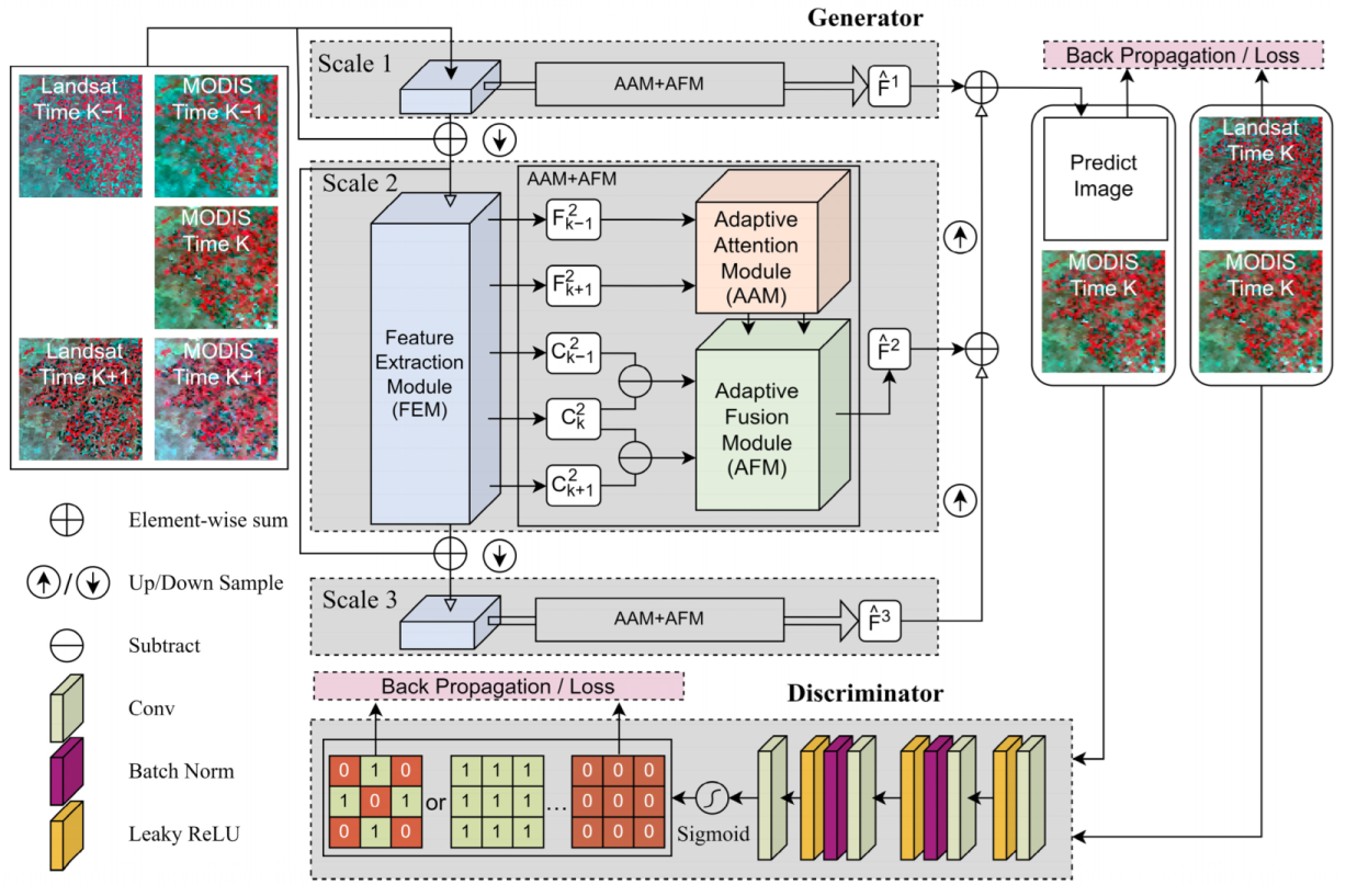
The overall structure of AMS-STF is shown in Figure 1. AMS-STF is based on GAN and consists of two parts: a generator and a discriminator. The generator employs a multiscale pyramidal network architecture to fully make use of both deep and shallow features. At each scale, the generator of AMS-STF is composed of three main submodules: a feature extraction module (FEM), an adaptive attention module (AAM), and an adaptive fusion module (AFM). The FEM is responsible for extracting the feature maps of remote sensing images. The AAM is a self-attention module based on residual blocks (RB) [37] and temporal adaptive blocks (TAB) [38]. It can effectively capture the temporal changes and enhance the multitemporal feature representations. By using deformable convolution (DConv) [39], the AFM can dynamically adjust the position and weight of the convolution kernel and enhance fusion performance for abrupt land covers. This module allows for more accurate use of features of land covers, and therefore leads to enhanced fusion performance for the sudden changes of land covers and higher-quality fusion images. GANs normally face some challenges, such as uncontrolled sample generation, unstable training, and mode collapse [40]. To improve the accuracy of the prediction results, this paper proposes a new discriminator network that combines Patch-GAN [41] and CGAN [40]. The original discriminator of GAN only outputs a general evaluation of the entire input image, which can result in inaccurate judgments for local regions with significant differences. The new discriminator addresses these issues and guides the generator to make more accurate predictions. Moreover, we design a loss function i.e., the weighted sum of adversarial loss and content loss, to speed up the convergence of the model and optimize the model performance. The rest of this section will describe the design of AMS-STF for its generator, discriminator, and loss function.

Figure 1.
Overall structure of AMS-STF.
2.2. Generator
The generator adopts the classic “encode-fusion-decode” structure to improve the information flow in different stages. In the encode stage, we use the FEM as the encoder to extract the feature maps of each input remote sensing image. During the fusion stage, the AAM and the AFM are used. The former is responsible for capturing more fine-grained spatiotemporal change information, and the latter is responsible for adaptively fusing feature maps in the temporal, spatial, and sensor dimensions. Together, these two modules enable the fusion stage to effectively integrate information from multiple sources and dimensions, resulting in improved STF results. In the decode stage, the decoder is responsible for the reconstruction of remote sensing images.
2.2.1. Overview of Multiscale Workflow
Inspired by the feature pyramid network and UNet [42], the generator of AMS-STF uses a multiscale structure to make full use of both deep high-dimensional features and shallow low-dimensional ones. The multiscale structure is effective to expand the receptive field of AMS-STF and adaptive to complex land covers, and hence can significantly improve the performance of image reconstruction.
As illustrated in Figure 1, three groups of multiscale features are extracted in the encode stage. They can be expressed by the following equation:
where and represent the LSHT image feature map and HSLT image feature map of scale at date , respectively; and represent the encoder of the LSHT image and HSLT image to scale , respectively. The extracted feature map is not only used for the fusion of the same layer, but also as the input of next stage. It should be noted that both and should be resampled to have the same size.
During the fusion stage, each group of multiscale features serves as the input to the fusion function, which can be expressed by the following equation:
where represents the fusion function of scale , and represents the feature map of the fusion output, which corresponds to scale at time .
In the decode stage, the high-level feature map is passed through the decoder to obtain an upsampled result, which is then added to the low-level feature map. This process continues recursively until the last scale is reached, resulting in a final set of feature maps that have been incrementally refined through the multiscale decoder. It can be expressed by the following equation:
where represents the result feature map of scale at time , and represents the decoder of scale . Finally, inspired by dropout-last [43], we use the structure of RB-Dropout-RB to generate the remote sensing image of the predicted date. This design benefits the generalization ability of the CNN networks for image reconstruction tasks.
2.2.2. Encoder and Decoder Structure
As the encoder, the feature extraction module (FEM) uses the basic components of RB. RB uses Leaky ReLU as the activation function and employs skip connections (elementwise-sum) to address the problems of gradient explosion and vanishing, and uses batch normalization to improve the convergence speed and alleviate the problem of poor activation function under deep neural network. To achieve a multiscale structure, the first convolution at each scale (excluding the first scale) uses a downsampling stride of 2. This enables the extraction of feature maps , , and at different scales, which are crucial for multiscale feature extraction. It is worth noting that we use a uniform encoder structure to extract features from remote sensing images obtained from different sensors. This implies that images captured by the same sensor can have identical representations during feature extraction. As a result, the encoder of each sensor shares network weights to streamline subsequent data processing and fusion. This approach ensures that different sensors are assigned distinct weights while maintaining consistent network architecture across different encoders.
In the decode stage, the decoder is responsible for fusing the above predicted feature maps and reconstructing the remote sensing images for the predicted date. UNet typically uses a deconvolution as the decoder, which may introduce unpleasant checkerboard artifact to the STF results [31]. To address the issue, our decoder uses a nearest neighbor interpolation algorithm for upsampling and an RB for removing artifacts, thus enabling the production of predicted images with better qualities. Using the decoder at scale 3 to scale 2 as an example, the predicted feature map is first upsampled to match the size by the nearest neighbor interpolation algorithm. After an RB, the result feature map is fused with the predicted feature map using element-wise sum.
2.2.3. Adaptive Attention Module Structure
In the fusion stage, in order to capture fine-grained spatiotemporal change information, we use an adaptive attention module (AAM) based on RB and temporal adaptive blocks (TAB) [38]. This implementation can well perceive temporal change information and contribute to more efficient and robust temporal modeling.
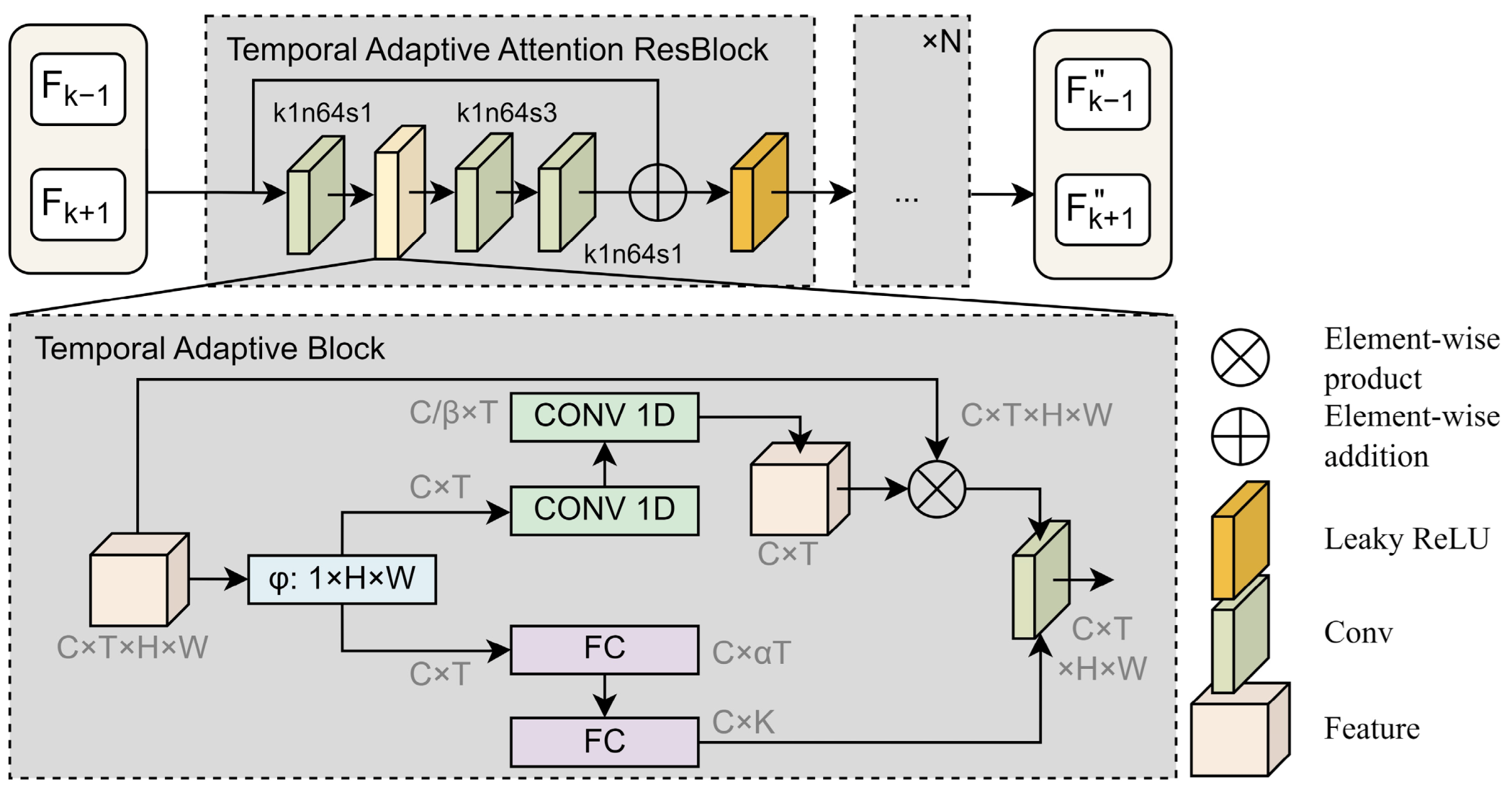
In this paper, the AAM is responsible for perceiving the fine feature maps and and produces the feature maps and , which are further enhanced with temporal feature information. The specific module structure is shown in Figure 2. The AAM consists of the Temporal Adaptive Attention ResBlock (TAAR). This block structure combines a bottleneck residual block with a TAB. By incorporating the TAAR, the AAM can effectively reduce computational resources while improving the ability of the model to perceive temporal changes and accuracy in processing time-series data.
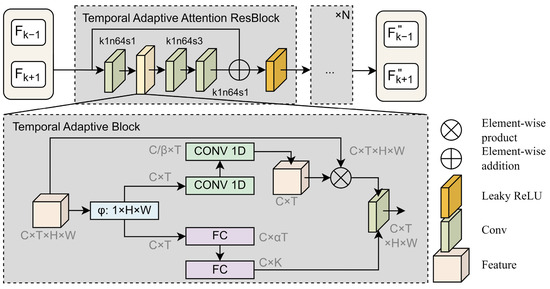
Figure 2.
The AAM structure, where k represents kernel size, n represents kernel, and s represents stride.
To provide a better understanding of the input data, let refer to continuous-time remote sensing image feature maps; represents the number of channels; and , , and represent the dimensions of time and space. The structure of the TAB is shown in the subfigure of Figure 2. It consists of a local branch and a global branch . The local branch aims to learn the sensitivity features of time and position, and the global branch aims to generate weight values with invariant location for convolution kernels. Finally, the information along the temporal dimension is adaptively computed through convolution, allowing for dynamic aggregation of temporal information. The formula for the TAB can be expressed as follows:
where represents convolutional operator, means element-wise product. Specifically, the local branch consists of two Conv-1D layers with ReLU activation functions. The first Conv-1D first reduces the number of channels from to , and then the second Conv-1D, together with the sigmoid activation function, generates temporal and positional sensitive feature weights. The global branch is location-invariant and generates the adaptive kernels through temporal information by two fully connected (FC) layers. One set of features is fed into the first FC layer, which increases the number of channels from to . After passing through the batch normalization layer, the features are then inputted into the second FC layer, which reduces the number of channels to . K is the size of the convolutional kernel.
2.2.4. Adaptive Fusion Module Structure
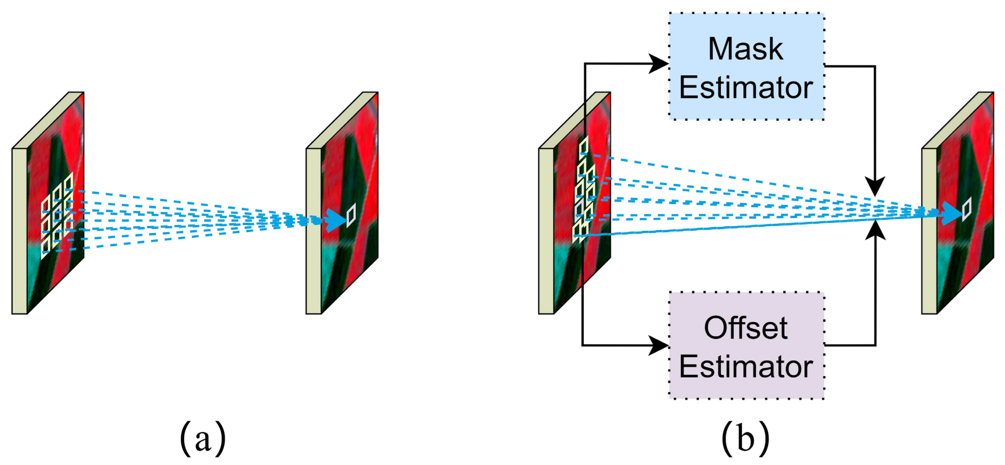
In this paper, we design an adaptive fusion module (AFM) for remote sensing images based on DConv to improve the fusion capacity of the STF model [39], which can be simply shown as Figure 3. In contrast to previous models that directly input the feature maps of MODIS to the convolutional layers, our approach utilizes a novel convolution technique combined with an attention mechanism. The developed AFM has three main components: deformable convolution operator, offset estimator, and mask estimator. Specifically, the deformable convolution operator uses an adaptive filter to vary the size and shape of convolution kernel, resulting in a flexible receptive field. The offset estimator dynamically adjusts the position of convolution kernel to selectively emphasize changing land cover patterns in different temporal and spatial contexts, resulting in enhanced fusion performance for abrupt land covers. The mask estimator generates a time-varying weight map from the MODIS feature map, which guides the convolution process of the Landsat feature. During the fusion stage, the developed AFM can adaptively fuse feature maps in the temporal, spatial, and spectral dimensions.
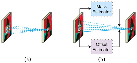
Figure 3.
The convolution method using two different types of convolution kernels: (a) normal convolution and (b) deformable convolution.
We begin by briefly describing the principle of the implementation of DConv. In this paper, we use deformable convolution V2 [44] as the operator. Suppose we have a convolution kernel with sampled positions, and let and denote the weight at the position and the offset originally specified by the convolution kernel, respectively. Let and denote the features at position from the input feature map and the output feature map , respectively. Then, the DConv operator can be expressed as:
where and denote the learnable offset and modulation scalar at the position, respectively. The modulation scalar lies in the range [0, 1], while is a real number with an unconstrained range. Therefore, we can input the learned and to make the convolutional kernel no longer present regular geometric shapes, but instead adaptively focus on the location of relevant objects, cleverly solving the problem of accumulation of pixel-independent information. DConv enlarges the receptive field of the convolutional kernel in STF tasks, which facilitates the adaptation to changing and complex local features, and more accurately utilizes object features to generate higher-quality fusion images.
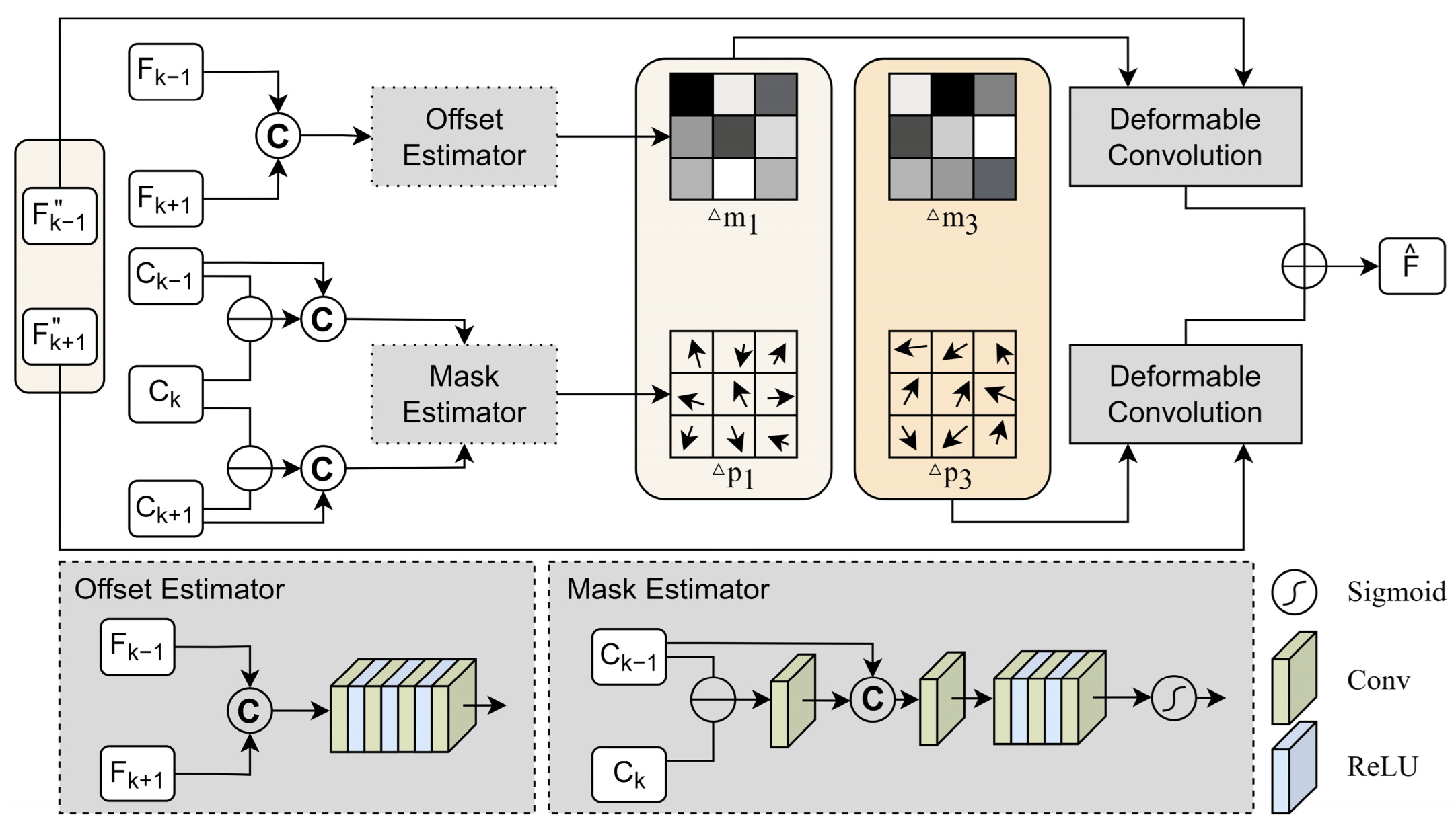
The specific implementation of the AFM is shown in Figure 4. The AFM demand imports two pairs of reference images and at time and , attention maps of HSLT image , and the LSHT image at a predicted time . Among them, L represents a certain scale within the range of ; t represents a specific time within the range of . Assume that the date to be predicted is day and the reference dates are day and day . One set is the reference date and the target date . The set contains the Landsat image feature for the reference date, the MODIS image feature for the target date, and the MODIS image change feature map for the reference date and the target date. Then, the AFM can be expressed by the following equation:
where Concat stands for concatenation, Offset stands for offset estimator, Mask stands for mask estimator, DConv stands for deformable convolution operator, and is the predicted feature map of the scale.
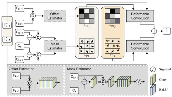
Figure 4.
The adaptive fusion module (AFM) structure.
The offset estimator generates the offset required for DConv by self-learning. The specific implementation details are shown by the Offset Estimator subfigure of Figure 4. To emphasize regions exhibiting significant temporal and spatial changes, the offset estimator concatenates feature maps of Landsat remote sensing images from two reference dates as input, and utilizes multiple convolution kernels and ReLU activation functions to extract temporal and spatial variation features. The Landsat data are preferred over MODIS as they provide more detailed information to support subsequent DConv operations.
The mask estimator is responsible for learning local feature variations in the temporal dimension and guiding the adaptive convolution kernel to eliminate sensor errors. The mask estimator achieves this by learning to generate a modulation scalar for DConv. To focus on the change in the temporal dimension of LSHT features, the MODIS feature map for the reference date t days is firstly subtracted from the feature map for the predicted date , and then a convolution is performed to obtain the change feature map for the two-day periods. The change feature map is then concatenated with to form a change feature map with LSHT image information, and the output channel is finally fed to the sigmoid layer through a structure like the offset estimator to obtain the temporal change modulation scalar required by the DConv.
Finally, the DConv operator uses a self-learning adaptive convolution kernel to generate the feature . The equation is shown in Equation (10), where the attention feature map is used as , the adaptive offset feature map is used as , and the temporal change modulation scalar is used as . As shown in Equation (11), the output feature maps from the two references are summed to reconstruct the predicted feature map for the scale.
2.3. Discriminator
The discriminator of the original GAN only outputs a true or false evaluation of the complete input image. This can lead to incorrect judgment values when using global metrics to measure local regions with large differences and fail to guide the generator to generate more accurate prediction results. To address these issues, this paper proposes a discriminator network that combines the Patch-GAN and CGAN approaches to generate more accurate prediction results. The specific details are shown in Figure 1, Discriminator.
The Patch-GAN discriminator can effectively address the aforementioned issues by outputting an matrix, called the confidence map, which consists of pixel values (0 or 1) representing the confidence level of the discriminator for a specific patch of the input image. The patch size in the Patch-GAN discriminator is equal to the receptive field size, which enables it to focus effectively on local details and generate sharper edges in the generated images.
CGAN is an effective approach for stabilizing the training process of traditional GAN networks. GAN training is unsupervised and can be highly unstable, leading to issues such as gradient vanishing or exploding. CGAN addresses these problems by introducing label constraints into the discriminator when input data need to be discriminated. In this way, CGAN improves the stability and convergence of the GAN training process. In this paper, the predicted image and the MODIS image on the predicted date are added as the label constraint during the discriminator working.
In this paper, we aim to concatenate the prediction and MODIS data in the channel dimension, as well as the Landsat and MODIS data, in order to obtain a full-false matrix output from the discriminator when the input is prediction and a full-true matrix output when the input is Landsat. We can express this process using the following equation:
where stands for the predicted date.
2.4. Loss Function
The loss function of AMS-STF is comprised of a weighted sum of adversarial loss and content loss, which ensures convergence of the model. The optimization objective of the adversarial loss is a minimax problem. The generator needs to minimize the loss value of the predicted output, i.e., minimize the loss, as follows:
The discriminator needs to accurately distinguish between the prediction and the target, so it needs to minimize the discrimination loss, as follows:
Rewriting Equation (14), it will look like this:
According to Equations (13) and (15), the adversarial loss of the generator and discriminator can be expressed as:
In addition, the generator loss consists of a combination of adversarial loss and content loss, and its expression can be represented by the following formula:
where is the weight coefficients of the adversarial loss. The content loss component uses a composite loss function that integrates perceptual loss, pixel loss, spectral loss, and vision loss. The content loss formula can be expressed as follows:
where is the weight coefficients of spectral loss function. Inspired by Tan [32], as shown in Equation (19), perceptual loss calculates the MSE spatial information loss of features after passing through the Sobel operator, which can effectively measure the degree of texture detail restoration in remote sensing images.
Pixel loss directly calculates the loss between the target and predicted values. It can be expressed as Equation (20):
Spectral loss and vision loss are defined according to the cosine similarity and multiscale structural similarity (MS-SSIM), respectively. They can be expressed as:
3. Experiments
3.1. Study Areas and Datasets
In the experiments, three open-source datasets are used to test the proposed model: the Coleambally Irrigation Area (CIA) and the Lower Gwydir Catchments (LGC) [45] located in New South Wales, Australia, as well as Tianjin [6] in China.
The CIA dataset consists of 17 pairs of cloud-free MODIS-Landsat images captured between October 2001 and May 2002. The primary land cover types in the dataset are forests, water, farmland, and bare land, which provide rich phenological change information. The spectral information in the images varies greatly with the seasons. The Landsat data were acquired using Landsat-7 Enhanced Thematic Mapper Plus (ETM+) with a spatial resolution of 30 m, while the MODIS data were sourced from MODIS Terra MOD09GA Collection 5. Both the MODIS and Landsat images were interpolated to a size of 2040 × 1720 at a 30-m resolution. It is worth mentioning that some Landsat images in the CIA dataset have missing data in corners. To avoid interference from these missing areas, the CIA dataset was cropped to a size of 2040 × 1360 during the training and evaluation processes.
The LGC dataset consists of 14 pairs of cloud-free MODIS-Landsat images captured between April 2004 and April 2005. The primary land cover types in the dataset are forests and farmland. During this period, a flood event occurred in mid-December 2004, which caused a large amount of farmland and land to be inundated. The floodwaters receded in late December, resulting in the images of the LGC dataset containing more sudden changes in land cover types. The Landsat data were acquired using Landsat-5 Thematic Mapper (TM), which has been atmospherically corrected using MODTRAN4. The MODIS data were also sourced from MODIS Terra MOD09GA Collection 5. Both the MODIS and Landsat images were interpolated to a size of 2720 × 3200.
The Tianjin dataset consists of 27 pairs of cloud-free MODIS-Landsat images captured between September 2013 and September 2019. The primary land cover types in the dataset are urban buildings, roads, and farmland. The Tianjin dataset contains images captured over a large time span, resulting in the observation of seasonal changes in urban landscapes and sudden changes in urban land cover types. The Landsat data in the dataset were acquired using Landsat-8 Operational Land Imager (OLI) with a spatial resolution of 30 m. The MODIS data were sourced from MODIS AQUA MOD02HKM. Both the Landsat and MODIS images in the dataset have been interpolated to a size of 1970 × 2100. It should be noted that the MODIS images in the Tianjin dataset exhibit noticeable band noise in the two short-wave infrared bands. Taking these issues into consideration, the two short-wave infrared bands will not be included in the experiment conducted.
3.2. Models and Evaluation Metrics
In order to verify the advanced nature of this model, we first compare the results of the AMS-STF model with those of six state-of-the-art STF models: ESTARFM [8], FSDAF [17], EDCSTFN [25], GAN-STFM [30], RSFN [32], and MLFF-GAN [31]. ESTARFM and FSDAF belong to the rule-based model, while the other four are deep learning-based models. In addition, to verify the effectiveness of each module, we also conducted ablation experiments on multiple modules in the AMS-STF model.
To ensure a fair comparison of the performance of each model, this paper employs four representative evaluation indicators: root mean square error (RMSE) [46], peak signal-to-noise ratio (PSNR), correlation coefficient (CC), and structural similarity (SSIM) [47].
3.3. Model Implementation and Settings
The implementation of AMS-STF is based on the PyTorch deep learning framework and the Python programming language. The experiments for both the proposed model and the comparative model were conducted on an Intel Xeon CPU E5-2680 v3 core with 128 GB of memory and four NVIDIA GeForce RTX 2080 Ti GPUs. All deep models were trained end-to-end using the same training dataset.
In the AMS-STF experiment, the CIA dataset of Landsat-MODIS images with 17 dates was divided into 15 groups, the LGC dataset with 14 dates of images was divided into 12 groups, and the Tianjin dataset with 27 dates of images was divided into 25 groups. Each dataset contained Landsat and MODIS images corresponding to three times: , , and . Two pairs of Landsat-MODIS images at and times were used as reference images, and the time k image was used as the predicted image. To ensure that the training and testing sets were not repeated, the images captured in the CIA dataset in 2002 (a total of 10 groups) were used for model training, and the images captured in 2001 (a total of 5 groups) were used for testing. The first seven sets of images in the LGC dataset were used as the training set, and the remaining five sets of images were used as the test set. The images from 2013 to 2017 in the Tianjin dataset (a total of 18 groups) were used for training, and the remaining data (a total of 7 groups) were used for testing.
The AMS-STF generator has 32, 64, and 128 output channels for each scale, respectively. Based on the recommendations in the TAM, the N is set to 1, the k is set to 3, and the s is set to 1 in the AAM. The dropout probability is set to 0.1. The Patch-GAN discriminator uses 3 layers, and the number of feature channels is set to 64. For the loss function, , . The Adam optimizer was used to train the model, with an initial learning rate of 0.0001 for the generator, a decay rate of 0.001, and a learning rate of 0.004 for the discriminator. During training, the batch size was set to 64, and the MODIS and Landsat images were cropped into small inputs of size 128 × 128 with a stride size of 128. Image slicing was performed dynamically during training. The number of iterations for all experiments was set to 200. The preparation of the dataset and hyperparameters for the other models were based on the specifications provided in published papers.
3.4. Experimental Results and Analysis
3.4.1. Contrast Experiments
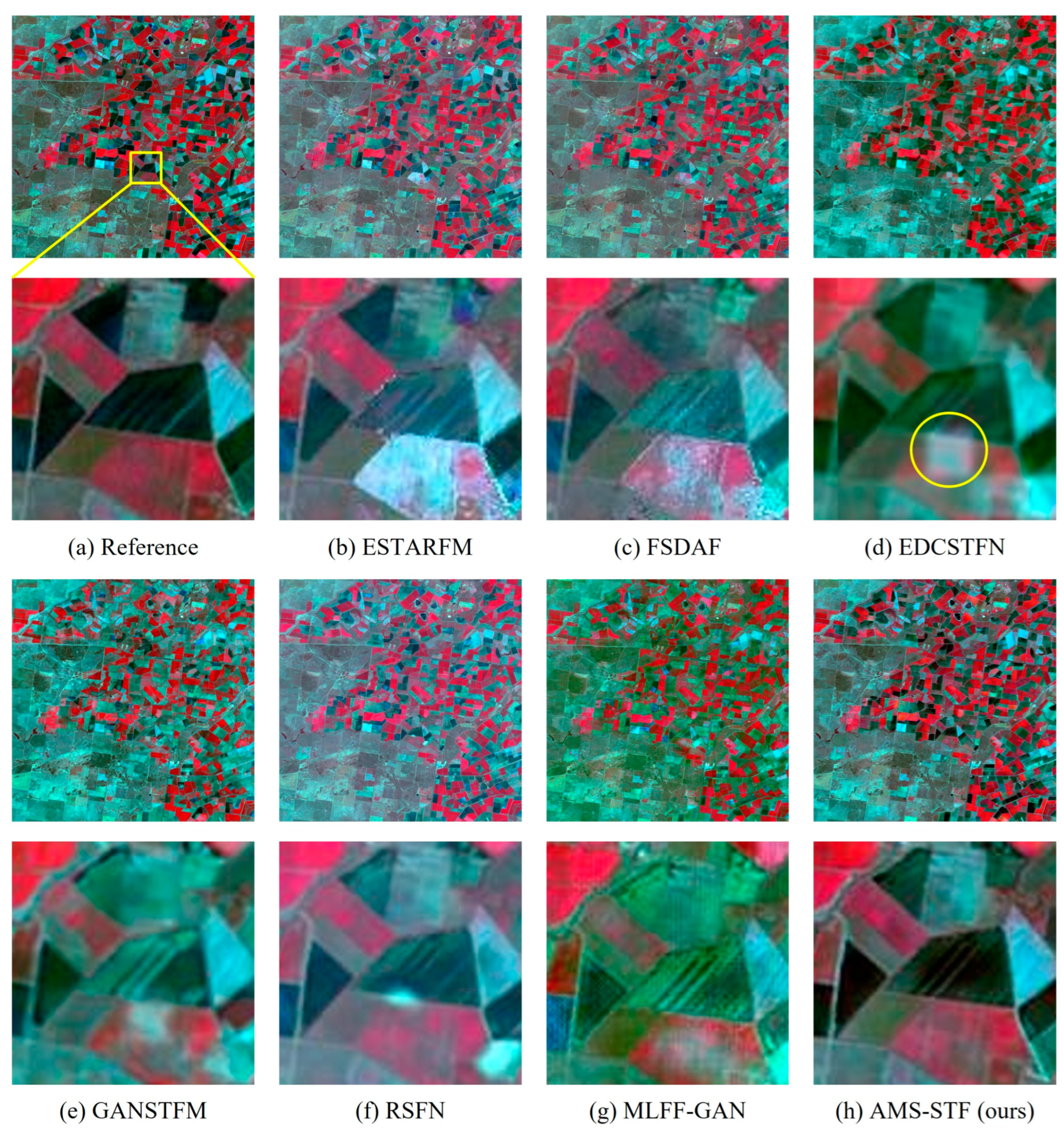
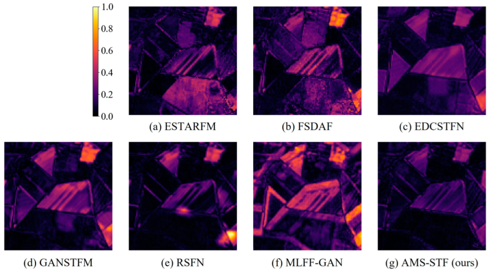
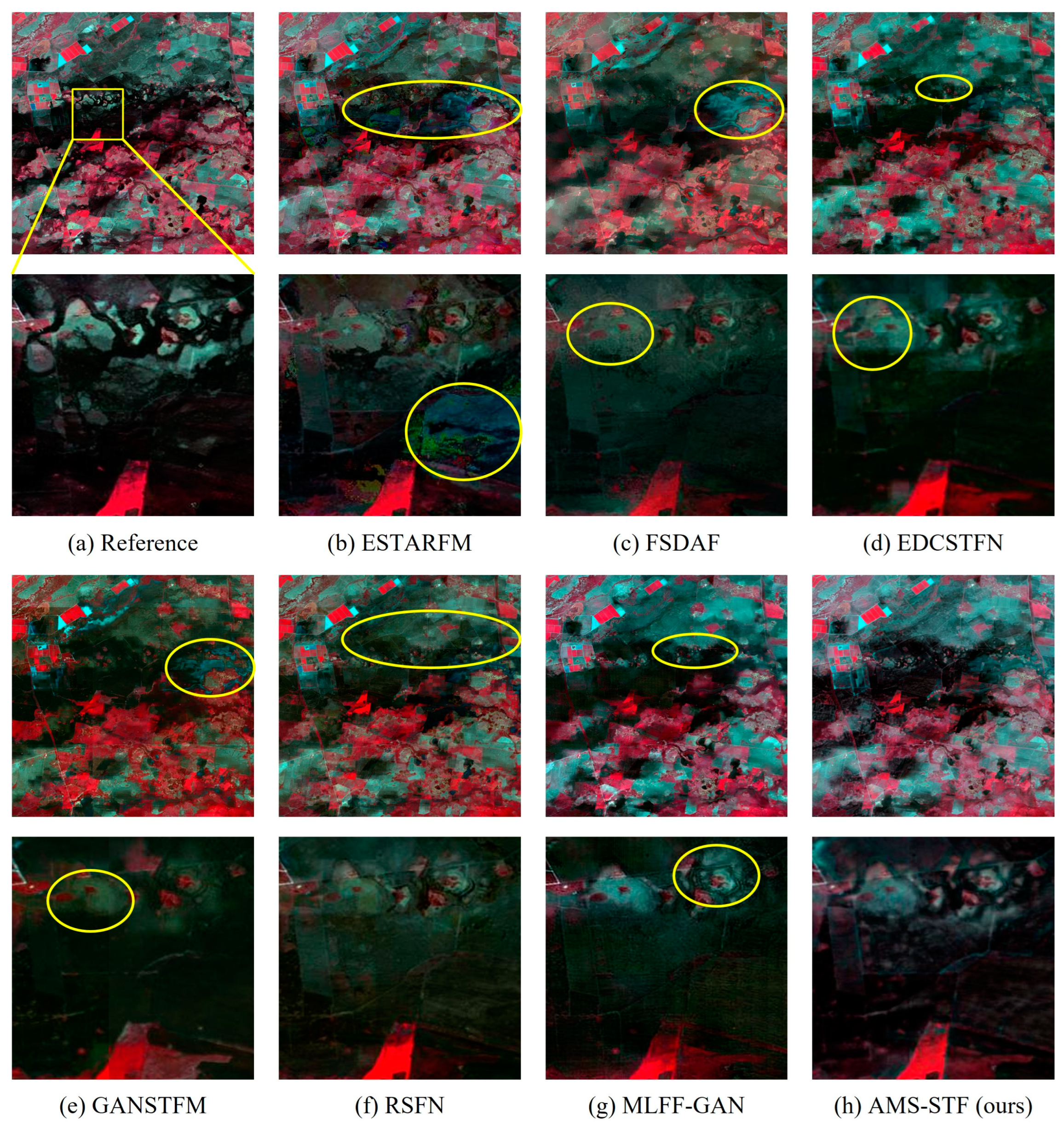
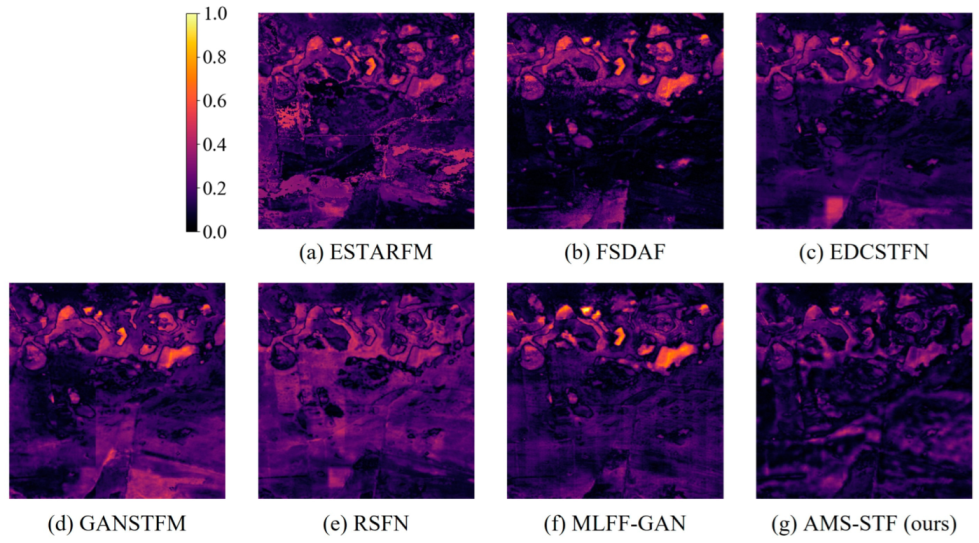
We conducted comparative experiments on three data sets. This section will show the results of each data set, as shown in Figure 5, Figure 6, Figure 7, Figure 8, Figure 9, Figure 10, Figure 11 and Figure 12. We select a set of test data in each dataset to visualize the experimental results, as shown in Figure 5, Figure 8 and Figure 11, respectively. Figure 5, Figure 8 and Figure 11 (top) show a thumbnail sketch of false-color (bands 4, 3, and 2) results from different models, while Figure 5a, Figure 8a and Figure 11a show the real Landsat image at a specific time. Figure 5, Figure 8 and Figure 11 (bottom) show a zoomed-in area in the yellow box corresponding to the top image. Figure 6, Figure 9 and Figure 12 show the sum of the absolute value differences of all bands between the ground truth and the prediction results of different models.

Figure 5.
Images of multiple models on the CIA. The top row is a local map, and the bottom row is a zoomed-in view of the area in the yellow square of the top row image.

Figure 6.
Visual images of difference maps in CIA.

Figure 7.
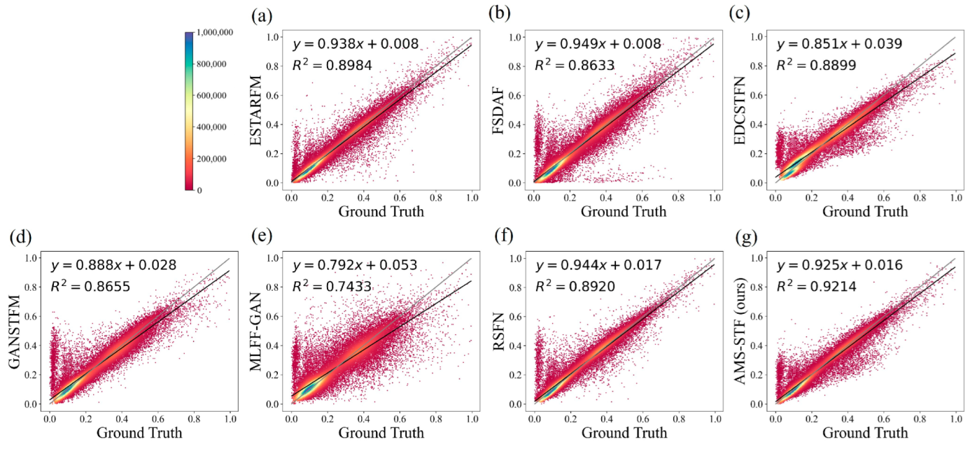
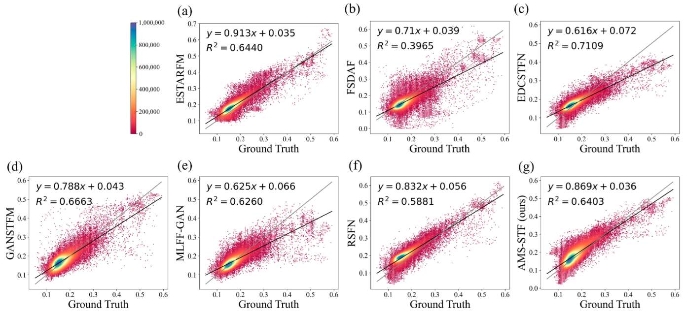
Scatter plots that compare observations with predictions on the CIA obtained by different models. The black line in the plots is the fitting line, and the grey line is the straight line with a slope of 1 for comparison. Different colors represent the density of points, where (a–f) are the results of ESTARFM, FSDAF, EDCSTFN, GANSTFM, MLFF-GAN, and RSFN models, respectively, and (g) is the result of our model.
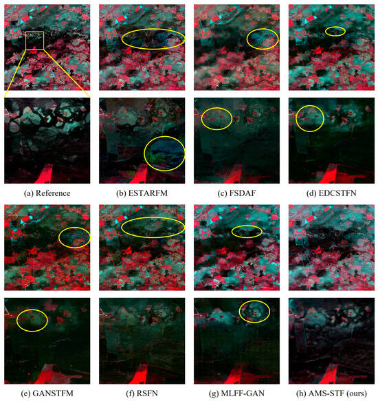
Figure 8.
Images of multiple models on the LGC. The top row is a local map, and the bottom row is a zoomed-in view of the area in the yellow square of the top row image.

Figure 9.
Visual images of difference maps in LGC.
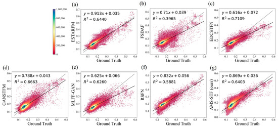
Figure 10.
Scatter plots that compare observations with predictions on the LGC obtained by different models. The black line in the plots is the fitting line, and the grey line is the straight line with a slope of 1 for comparison, where (a–f) are the results of ESTARFM, FSDAF, EDCSTFN, GANSTFM, MLFF-GAN, and RSFN models, respectively, and (g) is the result of our model.
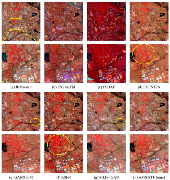
Figure 11.
Images of multiple models in the Tianjin dataset. The top row is a local map, and the bottom row is a zoomed-in view of the area in the yellow square of the top row image.
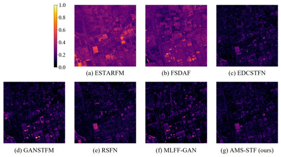
Figure 12.
Visual images of difference maps in Tianjin.
Figure 5 displays the prediction results of each model in the CIA dataset on 16 October 2001. It is evident that the proposed AMS-STF exhibits the best visual performance. We observed that the other STF models produce defective pixels due to the noise of MODIS. Among them, the ESTARFM and FSDAF models are most affected, resulting in a large area of unexpected noise. EDCSTFN and GAN-STFM generate grid-shaped noise like MODIS pixels. Models utilizing GAN, such as GAN-STFM, RSFN, MLFF-GAN, and AMS-STF, have achieved relatively good results in generating sharper edges. RSFN and MLFF-GAN produce unpleasant light spots and foggy noise, respectively. The proposed AMS-STF hardly exhibits such noise, and performs the sharpest land type edges, as shown in Figure 5h (bottom). Additionally, other STF methods have varying degrees of spectral distortion, particularly ESTARFM and RSFN. Compared to other models, AMS-STF fuses spectral information more tightly.
In Figure 6, the difference image corresponding to the enlarged image in the yellow box in Figure 5 is shown. Figure 6 shows more clearly the gap between the prediction results of each model and the real image. Surprisingly, MLFF-GAN presents the highest value in Figure 6, considering that this is because of the cumulative results of multiple bands, which proves that MLFF-GAN has serious spectral distortion in bands 1, 5, and 6. We find that EDCSTFN performs well on difference images, but still suffers from inaccurate prediction of the whole land, while AMS-STF performs better than EDCSTFN.
Figure 7 also shows the correlation of each model-predicted result image with the observed image for the CIA dataset on 16 October 2001. We found that the slopes of fitted lines for the ESTARFM, FSDAF, RSFN, and AMS-STF methods are all close to 1, and the R square of AMS-STF achieved the highest value. In general, according to the results of the scatter plot in Figure 7, the AMS-STF model has the best fitting result, which also indicates the superiority of the AMS-STF model.
Figure 8 displays the prediction results of each model in the LGC dataset on 28 December 2004. As mentioned in Section 3.1, the LGC area experienced flood disasters in mid-December 2004, and sudden changes in land cover types posed a challenge for the STF task. Because of the characteristics of LGC, we chose the dates when the floods occurred and then receded for visualization. Figure 8 (bottom) shows the predicted images of each model in the flood zone. We observed that most STF models exhibited some predictive ability for mutations, but the accuracy was still low. Among them, the image predicted by ESTARFM has serious noise, which greatly influences the fusion results for downstream applications. Although FSDAF has achieved better results than ESTARFM, it still cannot match deep learning-based models in predicting flood receding trends. As can be seen in Figure 8c, small pieces of spectral distortion appear in the FSDAF results. This phenomenon can also be observed (Figure 8 (top)) in the results fused by the other methods, except for MLFF-GAN and AMS-STF. From Figure 8 (bottom), the AMS-STF result successfully reveals the texture features of land divided by water flow, and shows better performance in the case of sudden land cover changes. In general, in terms of visual effects on the LGC dataset, the results of the GAN-based model performed better, and AMS-STF achieved the best results.
Similarly, we see through the results of the difference map in Figure 9 that AMS-STF achieves the dimmest result, which indicates that the difference between the results obtained by the AMS-STF model and the ground truth map is the smallest. RSFN shows relatively high values in the difference image, which might have resulted from spectral distortion. Through Figure 9, we can find that FSDAF has a good predictive ability for some ground object mutations and achieves a remarkable fusion performance. Figure 10 is the scatter plot result of the LGC on 28 December 2004. It shows that AMS-STF shows a better fitting effect.
Figure 11 displays the prediction results of each model in the Tianjin dataset on 3 February 2018. As mentioned in Section 3.1, the images in this dataset have a large imaging time span, and there are seasonal changes in urban landscapes and sudden changes in land cover types in some cities, which poses a greater challenge for STF. We found that in this dataset, the traditional models of ESTARFM and FSDAF perform poorly and suffer from severe spectral distortion effects. ESTARFM has obvious purple patches on the building plate, while the FSDAF image is generally reddish. The visual effects of deep learning-based models were similar in Figure 11 (top), and EDCSTFN and AMS-STF exhibited the best visual effects. Although RSFN recovers more detailed information, in the top of Figure 11f, the overall tone of the image is quite different from the reference image. Compared with EDCSTFN, GANSTFM, and MLFF-GAN, EDCSTFN still achieves the best results in remote sensing image fusion, which is the closest to the reference image. Comparing EDCSTFN with AMS-STF, the results of the two models have similar visual effects in the thumbnail sketch (Figure 11d,h (top)). However, upon zooming into the image and examining it closely (as shown in Figure 11d,h), it becomes apparent that the EDCSTFN approach produces a blurred surface texture that appears overly smoothed, and is not as visually pleasing. All in all, AMS-STF still managed to achieve the best visual performance among all methods on the Tianjin dataset.
Figure 12 shows the difference map of the Tianjin dataset. We found that the results based on the mathematical model have a relatively large overall difference, while the results of the model based on the deep learning method are only point-like high values. In the deep learning method, the difference map of the AMS-STF model achieves the best performance. This proves that the AMS-STF model is robust even on data sets with relatively large time spans.
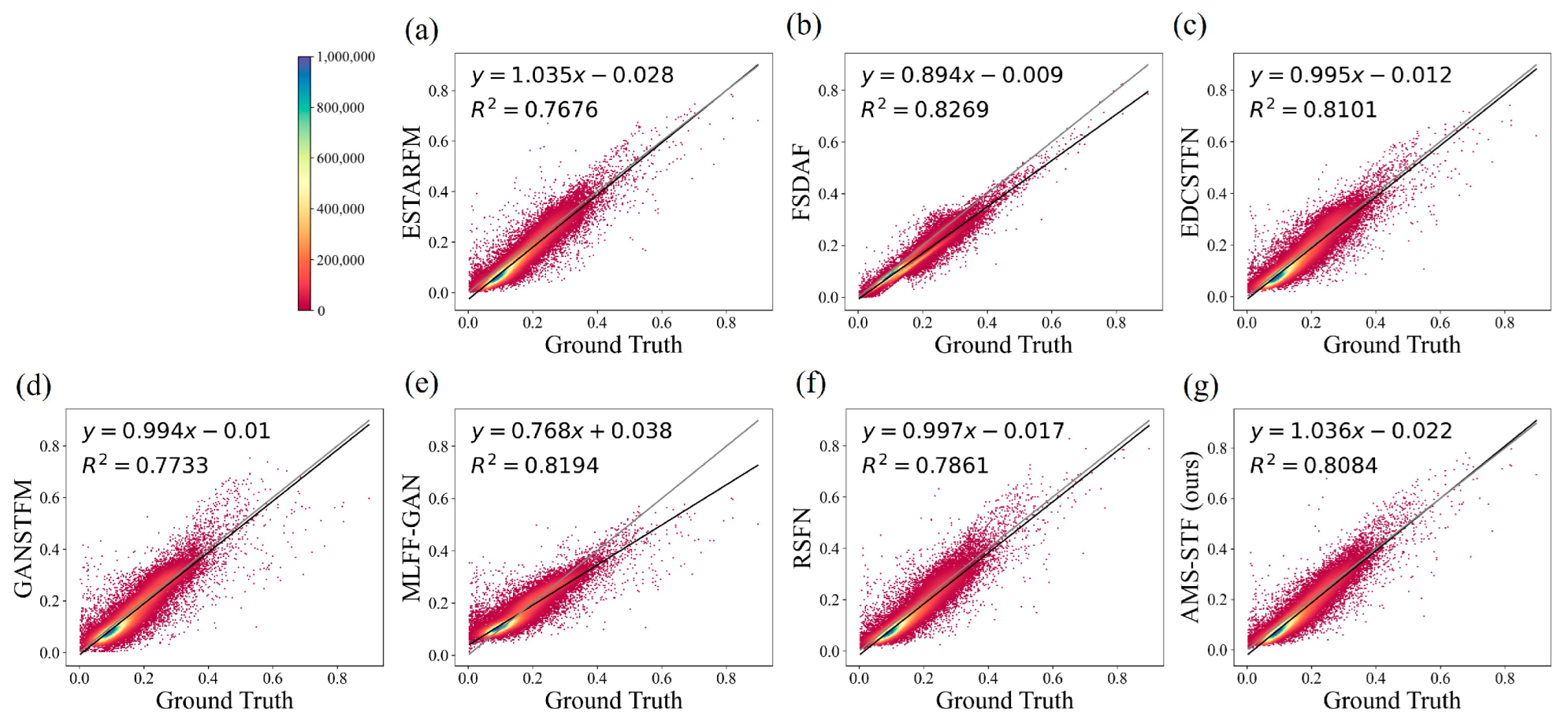
Figure 13 is the scatter plot result of the Tianjin dataset on 3 February 2018. We found that AMS-STF also achieved better results on the scatter plot. The slopes of the fitting lines of ESTARFM, EDCSTFN, GANSTFM, RSFN, and AMS-STF are all quite close to 1, while FSDAF, EDCSTFN, MLFF-GAN, and AMS-STF also have relatively high R squares. Overall, AMS-STF achieved good results and was only slightly inferior to EDCSTFN in terms of fitting performance on the Tianjin dataset.
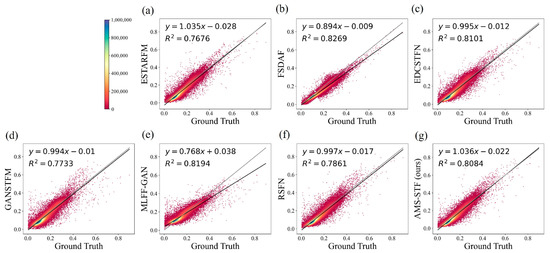
Figure 13.
Scatter plots that compare observations with predictions in the Tianjin dataset obtained by different models. The black line in the plots is the fitting line, and the grey line is the straight line with a slope of 1 for comparison. Different colors represent the density of points, where (a–f) are the results of ESTARFM, FSDAF, EDCSTFN, GANSTFM, MLFF-GAN, and RSFN models, respectively, and (g) is the result of our model. Table 1, Table 2 and Table 3 give the quantitative index evaluation of the three test groups in the CIA, LGC, and Tianjin datasets, respectively. For each evaluation metric, we use bold and underline to indicate the best results of the experiments. Based on Table 1, we observed that the models AMS-STF, ESTARFM, and RSFN, which input two high-resolution images of the reference date on the CIA dataset, performed well, with AMS-STF achieving the best result in most accuracy indicators. Table 2 shows that the AMS-STF model achieved better performance on the LGC dataset during floods, indicating a better ability to predict mutations. However, ESTARFM also exhibited good performance on some indicators, particularly in the test set to predict the date 20050129 DOY 029. Finally, Table 3 revealed that the prediction effect of various STF methods on the Tianjin dataset was not satisfactory, but the proposed AMS-STF model achieved leading performance in many indicators, especially in RMSE and PSNR. Overall, compared to existing STF models, AMS-STF exhibits better performance even under sudden ground changes, demonstrating robustness in multiple datasets with different characteristics.
3.4.2. Ablation Study
To verify the effectiveness of each module in the proposed method, we conducted three types of ablation experiments on three datasets and analyzed their impact on network performance by replacing or deleting different modules. Firstly, we deleted the AAM while keeping the rest of the structure unchanged to verify its influence on the network structure. Secondly, we replaced the AFM with ordinary convolution to verify the impact of deformable convolution on the network structure, while keeping the rest of the structure unchanged. Thirdly, we excluded the mask parameter of the AFM to verify the effect of the mask estimator, while keeping the rest of the structure unchanged. Finally, we explored the network structure without either the AAM or the AFM.
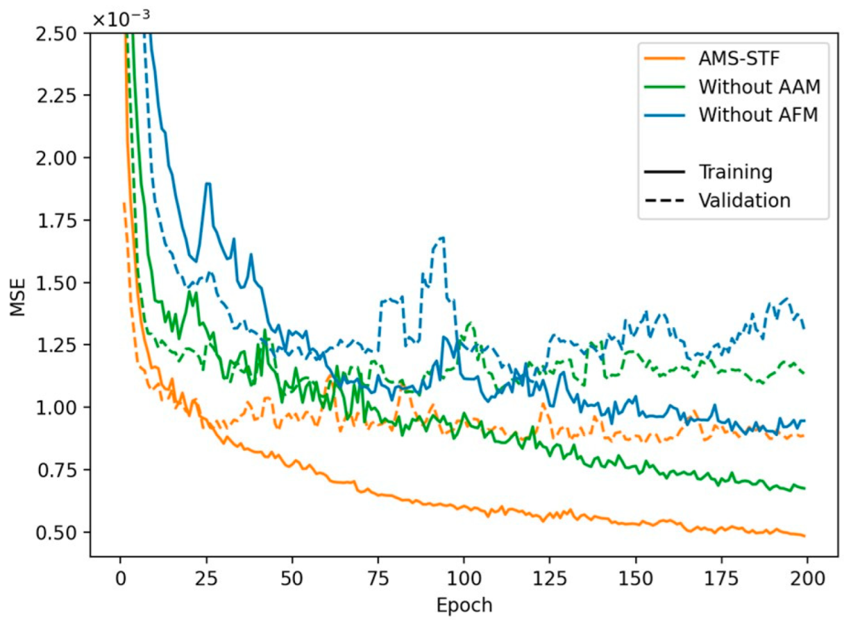
The quantitative comparison of the above experiments on the CIA, LGC, and Tianjin datasets is presented in Table 4, Table 5 and Table 6. The training and validation curves on the CIA dataset are shown in Figure 14.

Table 4.
Ablation experiment evaluation on CIA under AMS-STF. (“√” represents the use of this structure, and “×” represents no use of this structure).

Table 5.
Ablation experiment evaluation on LGC under AMS-STF. (“√” represents the use of this structure, and “×” represents no use of this structure).

Table 6.
Ablation experiment evaluation in Tianjin under AMS-STF. (“√” represents the use of this structure, and “×” represents no use of this structure).
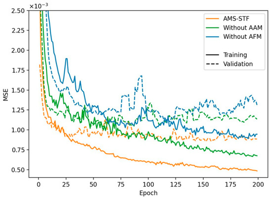
Figure 14.
Error curves of the ablation study in the CIA dataset.
We observed that both the AAM and AFM contributed to the improvement of the STF model, and the combination of the AAM and AFM yielded the best prediction results. Notably, the two structures with deformable convolution deleted exhibited the worst accuracy evaluation in most of the three datasets, indicating that AFM can effectively improve the accuracy of the STF model and enhance its robustness. Through comparison, we found that the network structure with AFM performed better when using AAM. The AAM provides more detailed feature change information, which can better guide deformable convolution to learn changes, especially enhancing its ability to predict mutations. Furthermore, we have discovered that the AFM demonstrates superior performance when using the mask estimator. This is attributed to the capability of the mask estimator to capture local feature variations in the temporal dimension, guiding the adaptive convolution kernel towards effectively eliminating sensor errors.
4. Discussion
This study proposes the AMS-STF and conducts experiments on three publicly available datasets: CIA, LGC, and Tianjin. Experiment results demonstrated that the fusion performance of various STF models on the CIA and LGC datasets is better than that on the Tianjin dataset. This might be caused by the following two reasons: first, the time span of the Tianjin dataset is long, and serious seasonal changes occur, while the time span of the CIA and LGC datasets is shorter and the changes in land cover are less drastic than in Tianjin. Second, most of the coverage areas in the datasets are urban areas, which are more spatially heterogeneous. Meanwhile, the LGC dataset covers surface abrupt changes caused by floods, which leads to lower prediction accuracy on flood dates than on other dates.
In contrast, AMS-STF consistently exhibits stronger stability compared to other models and consistently achieves the best performance across multiple experimental results. However, it is worth noting that ESTARFM and RSFN have demonstrated better results on specific indicators for certain dates within certain datasets. ESTARFM stands out by leveraging prior knowledge to propose various hypotheses for STF. While ESTARFM may have certain advantages in accuracy indicators on specific dates, its performance tends to fluctuate. On the other hand, RSFN excels in handling noise or cloud inputs and utilizes the attention subnet to learn weights. This allows RSFN to assign lower weights to noisy areas, thereby maintaining its robustness when dealing with data containing noise.
In AMS-STF, the mask estimator of the AAM specifically uses MODIS images from two reference dates as inputs to generate a time-varying weight map. However, the presence of noise in MODIS images can significantly impact the quality of the final fusion result. To address this issue, an alternative solution is to take Landsat images as additional inputs to the mask estimator. By considering both Landsat and MODIS data, it may be possible to reduce the influence of noise and enhance the overall quality of the fusion process.
From the visual results compared with various models, rule-based models such as ESTARFM and FSDAF both exhibit serious salt and pepper noise and peculiar spectral color differences. Even though ESTARFM achieves good results in accuracy evaluation, it is particularly affected by the quality of the input reference image. In contrast, deep learning-based models exhibit less salt and pepper noise in the visual results. The deep learning-based models demonstrate superior quantitative accuracy, underscoring its greater potential compared to traditional rule-based methods. But the smoothing effect caused by convolution is evident. The comparison of different deep learning-based models reveals that the GAN method excels in preserving texture information compared to pure CNN models, making it more suitable for STF. Therefore, we can conclude that AMS-STF excels in STF tasks, particularly demonstrating promising prospects in practical applications involving extended time spans or abrupt surface changes.
Through the results of contrast experiments, it can be found that the effect of using two pairs of reference images is better than that of using a pair of reference images to a certain extent. In fact, most algorithms only use the temporal variation information of MODIS, but ignore the temporal variation information between two Landsat images. This results in more data being used without fully exploiting the underlying information within the data. At the same time, in AMS-STF, the AAM is used to pay attention to the temporal change information between the two Landsat images at and , which makes up for this shortcoming well. This highlights the significance of modeling temporal changes in a reasonable manner. In the future, we will explore additional temporal modeling techniques, such as LSTM, to enhance the accuracy of our models.
Among the five learning-based methods, only EDCSTFN stands out as a non-GAN model. However, despite having the smallest number of parameters, previous experiments have revealed its unsatisfactory performance. On the other hand, MLFF-GAN and AMS-STF are both UNet-like models. The generator in AMS-STF benefits from the AAM and the AFM, resulting in half the number of parameters compared to MLFF-GAN, which provides a significant advantage. Although the generator and discriminator of AMS-STF do not have the fewest parameters, we introduce a small number of additional parameters to enhance the generalization ability of the model. The specific number of parameters is shown in Table 7. This aspect is crucial for its adaptability to real-world problems.

Table 7.
Parameters of five learning-based methods.
Through our ablation experiments, we have determined that the performance improvement achieved solely by using AAM is relatively limited. We attribute this limitation to the fact that our prediction process only uses two pairs of reference images. It is well-known that data augmentation can improve the accuracy of models, and inputting additional pairs of reference images may result in further improved fusion results. The AAM, which was originally developed for video action recognition tasks, supports the input of multiple dates. By concatenating the feature maps of multiple dates as input to the TAAR, additional reference dates can be incorporated into the model. By inputting the data of adjacent dates into the AFM, the images can be fused and combined using a weighted sum to achieve a more comprehensive and accurate result. In this way, additional reference image pairs can be integrated into the AMS-STF model to further improve its performance and expand its capabilities.
The ablation experiment results demonstrate the crucial role of AFM in enhancing the model’s performance. This might be resulted by three reasons. Firstly, the input of AFM is the fine image feature map, which contains more detailed information. Secondly, the position of the convolution kernel dynamically adjusts with the fine image feature map, enabling the model to focus more on the changing land covers. Additionally, the mask generated by the change in the MODIS image feature map indirectly migrates the temporal change and effectively resolves the artifacts problem. AFM exhibits remarkable adaptability to displacement and deformation, making it a promising choice for geological disaster scenarios like landslides. Additionally, AFM proves to be well suited for situations involving significant disparities in image resolution, as observed in the case of Sentinel-2 and Sentinel-3, where there exists a substantial 30-fold resolution difference.
5. Conclusions
This paper presents AMS-STF, a new GAN-based model for spatiotemporal fusion of remote sensing images. The generator employs two adaptive modules to address the temporal, spatial, and spectral differences in remote sensing image fusion. The discriminator uses a combination of CGAN and Patch-GAN to provide better constraints on local information reconstruction.
AMS-STF offers several clear advantages. First, using GAN in deep learning for remote sensing image fusion can reduce the smoothing effect caused by convolutional layers and enhance the texture information of the images. Second, the multiscale structure used in the generator can extract features and fuse them in a way that is compatible with the characteristic of varying object sizes, while also combining the benefits of shallow and deep features. Finally, both adaptive modules are applied for the first time in remote sensing image fusion tasks and have demonstrated their effectiveness. The AMS-STF model outperformed six other models in terms of robustness and accuracy, and its superior performance is attributed to the combination of AAM and AFM, as demonstrated in ablation experiments.
Author Contributions
Design of the method and experiment, X.P.; writing—original draft preparation, X.P.; data preprocessing, X.P. and M.D.; writing—review and editing, X.P., Z.A. and Q.X. All authors have read and agreed to the published version of the manuscript.
Funding
This research was funded by the National Key R&D Program of China (grant nos. 2017YFA0604300 and 2017YFA0604302), the Natural Science Foundation of China (grant nos. U1811464 and 41875122), Guangdong Top Young Talents (grant no. 2017TQ04Z359), and Western Talents (grant no. 2018XBYJRC004).
Data Availability Statement
The Coleambally Irrigation Area study site collection (CIA) used in this study is available at https://data.csiro.au/collection/csiro:5846v3 (accessed on 19 May 2014). The remote sensing data for The Lower Gwydir Catchment study site (LGC) are available at https://data.csiro.au/collection/csiro:5847v003 (accessed on 19 May 2014). The Tianjin city data are available at https://drive.google.com/drive/folders/1mnLe8JqNt0fq7DlJkzR0RFq7FjaxNjOO (accessed on 17 January 2020). The experimental codes are available at https://github.com/xxsfish/AMS-STF (accessed on 20 August 2023).
Conflicts of Interest
The authors declare no conflict of interest.
References
- Zhang, F.; Zhu, X.; Liu, D. Blending MODIS and Landsat Images for Urban Flood Mapping. Int. J. Remote Sens. 2014, 35, 3237–3253. [Google Scholar] [CrossRef]
- Miah, M.T.; Sultana, M. Environmental Impact of Land Use and Land Cover Change in Rampal, Bangladesh: A Google Earth Engine-Based Remote Sensing Approach. In Proceedings of the 2022 4th International Conference on Sustainable Technologies for Industry 4.0 (STI), Dhaka, Bangladesh, 17–18 December 2022; pp. 1–7. [Google Scholar]
- Johnson, M.D.; Hsieh, W.W.; Cannon, A.J.; Davidson, A.; Bédard, F. Crop Yield Forecasting on the Canadian Prairies by Remotely Sensed Vegetation Indices and Machine Learning Methods. Agric. For. Meteorol. 2016, 218–219, 74–84. [Google Scholar] [CrossRef]
- Luo, X.; Wang, M.; Dai, G.; Chen, X. A Novel Technique to Compute the Revisit Time of Satellites and Its Application in Remote Sensing Satellite Optimization Design. Int. J. Aerosp. Eng. 2017, 2017, e6469439. [Google Scholar] [CrossRef]
- Liao, C.; Wang, J.; Dong, T.; Shang, J.; Liu, J.; Song, Y. Using Spatio-Temporal Fusion of Landsat-8 and MODIS Data to Derive Phenology, Biomass and Yield Estimates for Corn and Soybean. Sci. Total Environ. 2019, 650, 1707–1721. [Google Scholar] [CrossRef]
- Li, J.; Li, Y.; He, L.; Chen, J.; Plaza, A. Spatio-Temporal Fusion for Remote Sensing Data: An Overview and New Benchmark. Sci. China Inf. Sci. 2020, 63, 140301. [Google Scholar] [CrossRef]
- Zhu, X.; Cai, F.; Tian, J.; Williams, T.K.-A. Spatiotemporal Fusion of Multisource Remote Sensing Data: Literature Survey, Taxonomy, Principles, Applications, and Future Directions. Remote Sens. 2018, 10, 527. [Google Scholar] [CrossRef]
- Gao, F.; Masek, J.; Schwaller, M.; Hall, F. On the Blending of the Landsat and MODIS Surface Reflectance: Predicting Daily Landsat Surface Reflectance. IEEE Trans. Geosci. Remote Sens. 2006, 44, 2207–2218. [Google Scholar] [CrossRef]
- Hilker, T.; Wulder, M.A.; Coops, N.C.; Linke, J.; McDermid, G.; Masek, J.G.; Gao, F.; White, J.C. A New Data Fusion Model for High Spatial- and Temporal-Resolution Mapping of Forest Disturbance Based on Landsat and MODIS. Remote Sens. Environ. 2009, 113, 1613–1627. [Google Scholar] [CrossRef]
- Zhu, X.; Chen, J.; Gao, F.; Chen, X.; Masek, J.G. An Enhanced Spatial and Temporal Adaptive Reflectance Fusion Model for Complex Heterogeneous Regions. Remote Sens. Environ. 2010, 114, 2610–2623. [Google Scholar] [CrossRef]
- Li, A.; Bo, Y.; Zhu, Y.; Guo, P.; Bi, J.; He, Y. Blending Multi-Resolution Satellite Sea Surface Temperature (SST) Products Using Bayesian Maximum Entropy Method. Remote Sens. Environ. 2013, 135, 52–63. [Google Scholar] [CrossRef]
- Huang, B.; Zhang, H.; Song, H.; Wang, J.; Song, C. Unified Fusion of Remote-Sensing Imagery: Generating Simultaneously High-Resolution Synthetic Spatial–Temporal–Spectral Earth Observations. Remote Sens. Lett. 2013, 4, 561–569. [Google Scholar] [CrossRef]
- Zhukov, B.; Oertel, D.; Lanzl, F.; Reinhackel, G. Unmixing-Based Multisensor Multiresolution Image Fusion. IEEE Trans. Geosci. Remote Sens. 1999, 37, 1212–1226. [Google Scholar] [CrossRef]
- Wu, M.; Niu, Z.; Wang, C.; Wu, C.; Wang, L. Use of MODIS and Landsat Time Series Data to Generate High-Resolution Temporal Synthetic Landsat Data Using a Spatial and Temporal Reflectance Fusion Model. J. Appl. Remote Sens. 2012, 6, 063507. [Google Scholar] [CrossRef]
- Zhang, W.; Li, A.; Jin, H.; Bian, J.; Zhang, Z.; Lei, G.; Qin, Z.; Huang, C. An Enhanced Spatial and Temporal Data Fusion Model for Fusing Landsat and MODIS Surface Reflectance to Generate High Temporal Landsat-Like Data. Remote Sens. 2013, 5, 5346–5368. [Google Scholar] [CrossRef]
- Wang, Q.; Atkinson, P.M. Spatio-Temporal Fusion for Daily Sentinel-2 Images. Remote Sens. Environ. 2018, 204, 31–42. [Google Scholar] [CrossRef]
- Zhu, X.; Helmer, E.H.; Gao, F.; Liu, D.; Chen, J.; Lefsky, M.A. A Flexible Spatiotemporal Method for Fusing Satellite Images with Different Resolutions. Remote Sens. Environ. 2016, 172, 165–177. [Google Scholar] [CrossRef]
- Liu, M.; Yang, W.; Zhu, X.; Chen, J.; Chen, X.; Yang, L.; Helmer, E.H. An Improved Flexible Spatiotemporal DAta Fusion (IFSDAF) Method for Producing High Spatiotemporal Resolution Normalized Difference Vegetation Index Time Series. Remote Sens. Environ. 2019, 227, 74–89. [Google Scholar] [CrossRef]
- Li, X.; Foody, G.M.; Boyd, D.S.; Ge, Y.; Zhang, Y.; Du, Y.; Ling, F. SFSDAF: An Enhanced FSDAF That Incorporates Sub-Pixel Class Fraction Change Information for Spatio-Temporal Image Fusion. Remote Sens. Environ. 2020, 237, 111537. [Google Scholar] [CrossRef]
- Gevaert, C.M.; García-Haro, F.J. A Comparison of STARFM and an Unmixing-Based Algorithm for Landsat and MODIS Data Fusion. Remote Sens. Environ. 2015, 156, 34–44. [Google Scholar] [CrossRef]
- Huang, B.; Song, H. Spatiotemporal Reflectance Fusion via Sparse Representation. IEEE Trans. Geosci. Remote Sens. 2012, 50, 3707–3716. [Google Scholar] [CrossRef]
- Song, H.; Liu, Q.; Wang, G.; Hang, R.; Huang, B. Spatiotemporal Satellite Image Fusion Using Deep Convolutional Neural Networks. IEEE J. Sel. Top. Appl. Earth Obs. Remote Sens. 2018, 11, 821–829. [Google Scholar] [CrossRef]
- Liu, X.; Deng, C.; Chanussot, J.; Hong, D.; Zhao, B. StfNet: A Two-Stream Convolutional Neural Network for Spatiotemporal Image Fusion. IEEE Trans. Geosci. Remote Sens. 2019, 57, 6552–6564. [Google Scholar] [CrossRef]
- Tan, Z.; Yue, P.; Di, L.; Tang, J. Deriving High Spatiotemporal Remote Sensing Images Using Deep Convolutional Network. Remote Sens. 2018, 10, 1066. [Google Scholar] [CrossRef]
- Tan, Z.; Di, L.; Zhang, M.; Guo, L.; Gao, M. An Enhanced Deep Convolutional Model for Spatiotemporal Image Fusion. Remote Sens. 2019, 11, 2898. [Google Scholar] [CrossRef]
- Li, Y.; Li, J.; He, L.; Chen, J.; Plaza, A. A New Sensor Bias-Driven Spatio-Temporal Fusion Model Based on Convolutional Neural Networks. Sci. China Inf. Sci. 2020, 63, 140302. [Google Scholar] [CrossRef]
- Goodfellow, I.J.; Pouget-Abadie, J.; Mirza, M.; Xu, B.; Warde-Farley, D.; Ozair, S.; Courville, A.; Bengio, Y. Generative Adversarial Networks. In Proceedings of the Advances in Neural Information Processing Systems 27 (NIPS 2014), Montreal, QC, Canada, 8–13 December 2014. [Google Scholar]
- Zhang, H.; Song, Y.; Han, C.; Zhang, L. Remote Sensing Image Spatiotemporal Fusion Using a Generative Adversarial Network. IEEE Trans. Geosci. Remote Sens. 2021, 59, 4273–4286. [Google Scholar] [CrossRef]
- Chen, J.; Wang, L.; Feng, R.; Liu, P.; Han, W.; Chen, X. CycleGAN-STF: Spatiotemporal Fusion via CycleGAN-Based Image Generation. IEEE Trans. Geosci. Remote Sens. 2021, 59, 5851–5865. [Google Scholar] [CrossRef]
- Tan, Z.; Gao, M.; Li, X.; Jiang, L. A Flexible Reference-Insensitive Spatiotemporal Fusion Model for Remote Sensing Images Using Conditional Generative Adversarial Network. IEEE Trans. Geosci. Remote Sens. 2022, 60, 5601413. [Google Scholar] [CrossRef]
- Song, B.; Liu, P.; Li, J.; Wang, L.; Zhang, L.; He, G.; Chen, L.; Liu, J. MLFF-GAN: A Multilevel Feature Fusion with GAN for Spatiotemporal Remote Sensing Images. IEEE Trans. Geosci. Remote Sens. 2022, 60, 4410816. [Google Scholar] [CrossRef]
- Tan, Z.; Gao, M.; Yuan, J.; Jiang, L.; Duan, H. A Robust Model for MODIS and Landsat Image Fusion Considering Input Noise. IEEE Trans. Geosci. Remote Sens. 2022, 60, 5407217. [Google Scholar] [CrossRef]
- Cao, H.; Luo, X.; Peng, Y.; Xie, T. MANet: A Network Architecture for Remote Sensing Spatiotemporal Fusion Based on Multiscale and Attention Mechanisms. Remote Sens. 2022, 14, 4600. [Google Scholar] [CrossRef]
- Shang, C.; Li, X.; Yin, Z.; Li, X.; Wang, L.; Zhang, Y.; Du, Y.; Ling, F. Spatiotemporal Reflectance Fusion Using a Generative Adversarial Network. IEEE Trans. Geosci. Remote Sens. 2022, 60, 5400915. [Google Scholar] [CrossRef]
- Song, Y.; Zhang, H.; Huang, H.; Zhang, L. Remote Sensing Image Spatiotemporal Fusion via a Generative Adversarial Network With One Prior Image Pair. IEEE Trans. Geosci. Remote Sens. 2022, 60, 5528117. [Google Scholar] [CrossRef]
- Zhu, Z.; Tao, Y.; Luo, X. HCNNet: A Hybrid Convolutional Neural Network for Spatiotemporal Image Fusion. IEEE Trans. Geosci. Remote Sens. 2022, 60, 2005716. [Google Scholar] [CrossRef]
- He, K.; Zhang, X.; Ren, S.; Sun, J. Deep Residual Learning for Image Recognition. In Proceedings of the IEEE Conference on Computer Vision and Pattern Recognition, Las Vegas, NV, USA, 27–30 June 2016. [Google Scholar]
- Liu, Z.; Wang, L.; Wu, W.; Qian, C.; Lu, T. TAM: Temporal Adaptive Module for Video Recognition. In Proceedings of the 2021 IEEE/CVF International Conference on Computer Vision (ICCV), Montreal, QC, Canada, 10–17 October 2021; pp. 13688–13698. [Google Scholar]
- Dai, J.; Qi, H.; Xiong, Y.; Li, Y.; Zhang, G.; Hu, H.; Wei, Y. Deformable Convolutional Networks. In Proceedings of the IEEE International Conference on Computer Vision (ICCV), Venice, Italy, 22–29 October 2017. [Google Scholar]
- Mirza, M.; Osindero, S. Conditional Generative Adversarial Nets. arXiv 2014, arXiv:1411.1784. [Google Scholar]
- Isola, P.; Zhu, J.-Y.; Zhou, T.; Efros, A.A. Image-to-Image Translation with Conditional Adversarial Networks. In Proceedings of the IEEE Conference on Computer Vision and Pattern Recognition (CVPR), Honolulu, HI, USA, 21–26 July 2017. [Google Scholar]
- Ronneberger, O.; Fischer, P.; Brox, T. U-Net: Convolutional Networks for Biomedical Image Segmentation. In Proceedings of the MICCAI 2015: 18th International Conference, Munich, Germany, 5–9 October 2015. [Google Scholar]
- Kong, X.; Liu, X.; Gu, J.; Qiao, Y.; Dong, C. Reflash Dropout in Image Super-Resolution. In Proceedings of the IEEE/CVF Conference on Computer Vision and Pattern Recognition, New Orleans, LA, USA, 18–24 June 2022. [Google Scholar]
- Zhu, X.; Hu, H.; Lin, S.; Dai, J. Deformable ConvNets v2: More Deformable, Better Results. In Proceedings of the IEEE/CVF Conference on Computer Vision and Pattern Recognition (CVPR), Long Beach, CA, USA, 15–20 June 2019. [Google Scholar]
- Emelyanova, I.V.; McVicar, T.R.; Van Niel, T.G.; Li, L.T.; van Dijk, A.I.J.M. Assessing the Accuracy of Blending Landsat–MODIS Surface Reflectances in Two Landscapes with Contrasting Spatial and Temporal Dynamics: A Framework for Algorithm Selection. Remote Sens. Environ. 2013, 133, 193–209. [Google Scholar] [CrossRef]
- Wald, L. Data Fusion. Definitions and Architectures—Fusion of Images of Different Spatial Resolutions; Presses de l’Ecole, Ecole des Mines de Paris: Paris, France, 2002; p. 200. [Google Scholar]
- Wang, Z.; Bovik, A.C.; Sheikh, H.R.; Simoncelli, E.P. Image Quality Assessment: From Error Visibility to Structural Similarity. IEEE Trans. Image Process. 2004, 13, 600–612. [Google Scholar] [CrossRef]
Disclaimer/Publisher’s Note: The statements, opinions and data contained in all publications are solely those of the individual author(s) and contributor(s) and not of MDPI and/or the editor(s). MDPI and/or the editor(s) disclaim responsibility for any injury to people or property resulting from any ideas, methods, instructions or products referred to in the content. |
© 2023 by the authors. Licensee MDPI, Basel, Switzerland. This article is an open access article distributed under the terms and conditions of the Creative Commons Attribution (CC BY) license (https://creativecommons.org/licenses/by/4.0/).

