Article

Spring Phenology Outweighs Temperature for Controlling the Autumn Phenology in the Yellow River Basin

1
School of Public Administration and Human Geography, Hunan University of Technology and Business, Changsha 410205, China
2
School of Resources and Environmental Sciences, Wuhan University, Wuhan 430079, China
*
Author to whom correspondence should be addressed.
Remote Sens. 2023, 15(20), 5058; https://doi.org/10.3390/rs15205058
Submission received: 31 August 2023 / Revised: 12 October 2023 / Accepted: 19 October 2023 / Published: 21 October 2023

Abstract

:
Recent research has revealed that the dynamics of autumn phenology play a decisive role in the inter-annual changes in the carbon cycle. However, to date, the shifts in autumn phenology (EGS) and the elements that govern it have not garnered unanimous acknowledgment. This paper focuses on the Yellow River Basin (YRB) ecosystem and systematically analyzes the dynamic characteristics of EGS and its multiple controls across the entire region and biomes from 1982 to 2015 based on the long-term GIMMS NDVI3g dataset. The results demonstrated that a trend toward a significant delay in EGS (p < 0.05) was detected and this delay was consistently observed across all biomes. By using the geographical detector model, the association between EGS and several main driving factors was quantified. The spring phenology (SGS) had the largest explanatory power among the interannual variations of EGS across the YRB, followed by preseason temperature. For different vegetation types, SGS and preseason precipitation were the dominant driving factors for the EGS in woody plants and grasslands, respectively, whereas the explanatory power for each driving factor on cultivated land was very weak. Furthermore, the EGS was controlled by drought at different timescales and the dominant timescales were concentrated in 1–3 accumulated months. Grasslands were more significantly influenced by drought than woody plants at the biome level. These findings validate the significance of SGS on the EGS in the YRB as well as highlight that both drought and SGS should be considered in autumn fall phenology models for improving the prediction accuracy under future climate change scenarios.

1. Introduction

Vegetation phenology is a crucial aspect of understanding how plants and ecosystems respond to the surrounding environmental conditions [1,2]. The timing of phenological events not only reflects the changes in terrestrial ecosystems but also enables the monitoring of climate change across various regions and scales [3,4]. Currently, plenty of investigations utilizing satellite remote sensing data and in-situ records have considerably advanced our comprehension of spring phenology (start of growing season, SGS) in recent decades [5,6,7,8] and a unanimous conclusion has been reached that temperature is the first key to controlling changes in SGS [9]. By contrast, there have been significant works pointing to the spatial pattern of autumn phenology (end of growing season, EGS) trends that are much more heterogeneous than that of SGS. For example, a delayed trend of EGS over the past decades has been found across North America [10], Eurasia [11] and China [12] by using satellite data, yet, an advanced trend has been observed in EGS in Siberia, Central Eurasia [13] and the Great Lakes region of Central Asia [14]. Furthermore, inconsistent trends in EGS have been observed across different study periods [15,16] and there is no trend in EGS during the global warming hiatus [17]. Though the trends of the seen changes are not yet clear, earlier studies indicate the variation in EGS is closely associated with climate change [18,19] and highlight that it could play a fundamental role in controlling inter-annual fluctuations in ecosystem productivity as well as in regulating the nutrients cycle [20,21,22]. Therefore, the investigation of EGS dynamic changes and their corresponding driving factors can help enrich our understanding of the response and feedback mechanisms of terrestrial ecosystems to climate change in the context of continuous global warming and is also of great significance in improving the accuracy of autumn phenology models.
From the perspective of plant physiology, the photoperiod is widely recognized as the principal factor influencing EGS. Multiyear experiments from controlled environments (e.g., growth chambers) have suggested that leaf senescence would be triggered when the photoperiod is below the critical threshold [23]. It has been discovered that leaf senescence in regions with severe winter conditions is heavily influenced by photoperiods [24] but there are no consistent conclusions in other regions. Additionally, a growing number of research speculates on the coregulatory effects of the photoperiod and temperature on EGS [25,26]. As demonstrated by Worrall [27], when the photoperiod shortens and temperatures decrease in autumn, an abscission zone begins to form at the base of the petiole, leading to the degradation of plant chlorophyll [28]. Meanwhile, some studies set out to focus on investigating the impacts of temperature on EGS, and pieces of evidence have proven that warming played a critical role in regulating EGS [29,30], especially for vegetation in lower altitude regions [31]. Recent studies have also proposed that the impacts of diurnal and night-time warming on EGS vary across different regions [32,33]. However, the spatial and temporal variations in EGS could not be fully explained by temperature, particularly in the water-constrained regions [34]. Precipitation controls the EGS by indirectly affecting the thermal requirement, nutrient availability and soil water content [35,36]. For instance, Zhang et al. [37] found that preseason precipitation had a more pronounced influence on EGS compared to SGS in Northern China. Liu et al. [13] demonstrated that preseason precipitation plays a dominant and positive role in the grassland across the Northern Hemisphere (NH), whereas the sensitivity of EGS to precipitation in the NH gradually decreased from 2001 to 2015 [15]. It follows that these intricate response patterns have given rise to significant heterogeneity in the relationship between the climate and EGS.
Although extensive research has been conducted on the impact of climate-forcing factors such as temperature, precipitation and photoperiod on the EGS (ecosystem goods and services), there is still a significant gap in understanding the effects of drought on EGS in different periods [38]. Drought, being a highly intricate climate phenomenon, has severe implications on vegetation growth, productivity and mortality as it disrupts the water network of vegetation roots [39,40,41]. Several studies on grasslands in China and Canada have observed that drought in summer and autumn advanced EGS [42,43], while the opposite result was found in deciduous trees in Northeastern USA [26,44]. According to a recent study, the advance of EGS in alpine and temperate grasslands in China is influenced more by meteorological drought than by temperature [45]. Moreover, Ge et al. [46] suggested that there is a strong link between EGS and drought, with the EGS of farmland and forest exhibiting considerable vulnerability to drought at monthly and annual scales, respectively. The impact of drought on EGS is evident, although it differs based on the region and vegetation type. Therefore, it is crucial to examine the influence of drought on EGS. Furthermore, considering the notable rise in the intensity and frequency of drought events in recent years, with further expected intensification in the coming decades, particularly in semiarid regions [47], a comprehensive exploration of the correlation between these factors could offer valuable insights into understanding future phenology in response to climate change.
Generally, the cycle of plant phenology is commonly considered as an integrated indicator, where the timing of each phenological stage depends, to some extent, on the development of the previous stage(s) [48,49]. This means that, in addition to being regulated by environmental factors, the EGS also has a strong dependence on the growth status of vegetation prior to EGS [16]. Previous studies have observed that an earlier SGS is associated with an earlier EGS in both temperate deciduous forests and grasslands of the NH. [13,18]. The mechanisms of interaction among phenological events might be attributed to excessive water consumption during earlier SGS, which leads to summer drought, ultimately causing the corresponding advancement of EGS. On the other hand, it is believed that carbon capture increases after earlier SGS, which inhibits the capacity of photosynthesis and constrains the productive season length in sink-limited plants [50]. Moreover, Peng et al. [51] reported that among various potential driving factors, SGS played a prominent role in influencing changes in EGS in the Tibetan Plateau. However, this is not unanimously recognized by other research results, and the importance of the effect of SGS on EGS varies between analyses. For instance, Ren et al. [52] and Fu et al. [53] discovered a notable negative correlation between EGS and SGS in temperate grasslands of the NH and the northeastern Greater Khingan. Evaluations conducted at the site level have also concluded that the contribution of SGS to EGS is relatively smaller compared to climatic factors. Furthermore, the EGS of tree species in China was found to be associated more with the combined effects of climate and phylogeny than with SGS [54].
The results mentioned above indicate that the responses and sensitivities of autumn phenology to environmental cues and SGS were diverse. This diversity further complicates the task of identifying the dominant factor that contributes to variations in EGS. Although previous studies have made strenuous efforts to explore the relationship between EGS and driving factors, research on quantifying the contributions of these factors to EGS remains challenging. Even though most studies attempt to quantify the control of the driving factor in the dynamic changes in EGS based on a linear hypothesis [55,56], in reality, the response of the ecosystem to factors has been shown to be nonlinear due to the existence of complex interactions and feedback mechanisms among the driving factors [57]. Therefore, how to effectively quantify the independent contributions of driving factors to the dynamic changes of EGS still needs further research.
The Yellow River Basin (YRB), the second-largest river basin in China, plays a pivotal role in China’s ecological security. The violently undulating terrain, complex and diverse landform types and various hydrothermal combinations contribute to the development of a wide range of vegetation types. Works in the literature have recorded that the temperature in the YRB has increased significantly, while precipitation has shown an insignificant decreasing trend since the 1950s [58,59]. Meanwhile, the drought coverage, frequency and trend in the whole basin have been constantly increasing [60]. Therefore, the YRB is an ideal region to investigate how autumn phenology responds to multiple environmental factors. Previous studies used different types of data to analyze the phenology of the Yellow River Basin and found that the delay in vegetation EGS in the region over the past three decades was regulated by the preseason night-time temperature [61] but since 2000, the influence of precipitation on EGS has become the dominant factor [62]. However, these studies were either limited to the study of climate effects on phenology or the analysis of phenology response to potential driving factors based on linear, trend and correlation methods, while ignoring the impact of spatial heterogeneity of factors, which has an important influence on the spatial distribution of phenology. Thus, the primary goals of this study were to (1) explore the spatial-temporal variation trend of EGS in the YRB and different vegetation types from 1982 to 2015; (2) unravel the relationship between each driving factor and EGS; (3) quantitatively measure the contribution of each driving factor on the EGS distribution and distinguish the disparities among vegetation types; and (4) investigate the effects of drought on the EGS.

2. Materials and Methods

2.1. Research Area

The YRB (95°53′–119°5′E, 32°10′–41°50′N) encompasses four geomorphic units from west to east and covers approximately 7.83% of China’s land area. One significant climatic characteristic of YRB is the marked temperature variation. From the southwest to the southeast, temperatures change from cold to warm, with an annual mean temperature ranging between −7 °C and 14 °C. Under the control of the typical monsoon climate, the mean annual precipitation is approximately 476 mm, with summer being the wettest period [51]. As a consequence of the complex terrain as well as varying hydrothermal conditions, the vegetation types in the YRB can be classified into five categories: deciduous broad-leaved forest (DBF), deciduous coniferous forest (DNF), evergreen coniferous forest (ENF), cultivated vegetation (CV) and grassland (Figure 1).

2.2. Dataset Sources

The third-generation NDVI (NDVI3g) used in this study was released by the Global Inventory Monitoring and Modeling Study (GIMMS) (https://ecocast.arc.nasa.gov/data/pub/gimms/3g.v1/ (accessed on 10 July 2022)). This dataset covered the period from 1982 to 2015, with a spatial resolution of 1/12 degree and 15-day time steps. The various negative effects and noises associated with the change in satellite sensors, orbital drift, atmospheric interference and nonvegetation dynamics were eliminated [63].
Data on gridded daily air temperature (Tem) and precipitation (Pre), with a resolution of 0.5° × 0.5°, were collected from the China Meteorological Administration for the period 1982–2015. The gridded daily absorbed downward shortwave solar radiation (Ssd) data with a resolution of 0.1° × 0.1° were provided by the China Meteorological Forcing Dataset [64]. Both of the two datasets have been applied in recent climate change and phenological research.
The vegetation type raster map was compiled by the Chinese Academy of Sciences (https://www.resdc.cn/data.aspx (accessed on 21 October 2023)).
The standardized precipitation and evapotranspiration index (SPEI), which is a multiscalar drought index that measures the imbalance between precipitation and potential evapotranspiration, was obtained from the SPEIbase v.2.5 (http://spei.csic.es/database.html (accessed on 18 April 2022)). The gridded monthly data have a spatial resolution of 0.5° [65]. SPEI on 1–12 month timescales and were utilized to capture the potential impacts of drought on vegetation growth cycles.
To fulfill the identical spatial resolution of the NDVI dataset, the resampling method was applied to all datasets analyzed in this study.

2.3. Extraction of Phenology Metrics

The original NDVI was processed using the Savitzky–Golay (SG) filter to eliminate abnormal values caused by residual noise. Considering that the bare soil and sparse vegetation will have a certain influence on the trend of NDVI, for subsequent analysis, pixels that displayed a mean annual NDVI lower than 0.1 over the entire duration of 34 years were excluded [66].
The Polyfit-Maximum method was employed to extract phenological information (SGS and EGS) from the NDVI time series [67,68]. The specific steps were as follows:
First, for every pixel, the average seasonal NDVI curves at 15-day intervals from 1982 to 2015 were calculated. Then, we applied the formula (Equation (1)) to ascertain the relative change.
N D V I r a t i o t = ( N D V I t + 1 N D V I t ) / N D V I t
where NDVIratio(t) is the relative change in NDVI and t is the time (temporal resolution of 15 days). We then detected the time, t, with the maximum NDVIratio and used the corresponding threshold, NDVI(t), to determine the SGS; similarly, the minimum NDVIratio at time, t, was detected and the corresponding threshold, NDVI(t+1), was used to determine the EGS. Additionally, the time series of NDVI data were filtered using an inverted 6-degree polynomial function (Equation (2)) [69].
N D V I t = a + a 1 t 1 + a 2 t 2 + a 3 t 3 + a 4 t 4 + a 5 t 5 + a 6 t 6
where t is the Julian days. a1, a2, a3…, a6 are the fitted coefficients obtained from the least square regression.

2.4. Statistics and Analysis

2.4.1. Trend Detection

The Theil–Sen median method was used to explore the magnitude of the trend in EGS across the YRB from 1982 to 2015 at the pixel level.
Q = m e d i a n x j x i j i       1 i < j n
where Q is the Sen’s slope; xj and xi indicate the sequence value at time, j and i, respectively; the median is calculated from all pairs of observations in the time series. Q > 0 suggests that the EGS is delayed, and Q < 0 suggests that the EGS is advanced. The Mann–Kendall nonparametric statistical test was used to determine the significance of the EGS variation trend [70].

2.4.2. Correlations between EGS and Driving Factors

The objective of this study was to investigate the impact of climatic factors on EGS through the implementation of a partial correlation analysis. This approach was adopted specifically to enable us to investigate the relationship between EGS and a single climatic factor and eliminate the compound effects of the other remaining factors [13]. Typically, the advance or delay of phenological events is influenced by their regulators over a specified period [71]. It has been found that the climatic conditions in the several days/months prior to phenological events play a pivotal role in the development of vegetation phenology [58,59]. Therefore, the term “preseason” is used to refer to a specific period before a phenological event [72]. Taking temperature as an example, for each pixel, the preseason in this study was defined as the period (with a one-month time step) before the averaged multiyear EGS date for which the partial correlation coefficient between EGS and mean temperature was highest, controlling for total precipitation, total solar radiation and SGS [73,74]. The precipitation and radiation involved here were for the same period as the mean temperature. According to past studies, the maximum range of this period for each pixel was set from June to the multiyear average date of EGS [51,66]. The preseason for precipitation and solar radiation was identified in the same way. Similarly, to determine the impact of SGS on EGS, a partial correlation analysis of SGS and EGS was implemented as well as controlling for preseason climate variables.

2.4.3. Geographical Detector Model

A GDM is a type of spatial statistical method that detects the consistency of spatial distribution patterns between dependent variables and independent variables through spatial heterogeneity and that reveals the relative importance of independent variables in explaining spatial differentiation [75]. This method has shown good performance in recent research applications in various fields [76,77]. In this study, we examined the explanatory power of climate factors and SGS on EGS by utilizing preseason climate factors and SGS as independent variables and the change rate of EGS as a dependent variable. The formula for the explanatory power of each factor is as follows:
q x = 1 h = 1 L N h σ h 2 N σ 2 = 1 S S W S S T
where qx (∈[0, 1]) is the power of the driving factor x; h = 1,…, L is the stratum (category) of EGS for driving factor x. The physical meaning of the q value is that the independent variable x explains 100 × q% of the dependent variable EGS; Nh and N are the total sample numbers of the h stratum and overall period (1982–2015), respectively; σ h 2 and σ 2 are the variances of EGS in the h stratum and overall period, respectively. SSW and SST are the number, variance and sum of the variance of units in h and the whole area, respectively.

2.4.4. Cumulative Effects of Drought on EGS

The Pearson correlation analysis was employed to assess the impact of drought on EGS, aiming to determine the cumulative effect [78]. Specific steps were represented as follows: First, we acquired the month of EGS for every pixel across the period of 1982–2015 (EGSm) and then extracted 12 monthly SPEI values corresponding to the EGSm from 1- to 12-month SPEI in each year. Next, the Pearson correlation was used to explore how EGS responded to accumulated SPEI at a 1- to 12-month time scale. Subsequently, all correlation coefficients between EGS and SPEI were considered to determine the cumulative effect at this pixel (Equation (5)). Finally, we retained the absolute maximum correlation coefficient (Rmax) along with the corresponding SPEI time scale in which Rmax was achieved (Equation (6)).
R j = c o r r E G S , S P E I j       1 j 12
R m a x = max R j       1 j 12
where Rj is the Pearson correlation coefficient between EGS and SPEI, j is the accumulated time from 1- to 12-month SPEI and Rmax is the maximum value of Rj.

3. Results

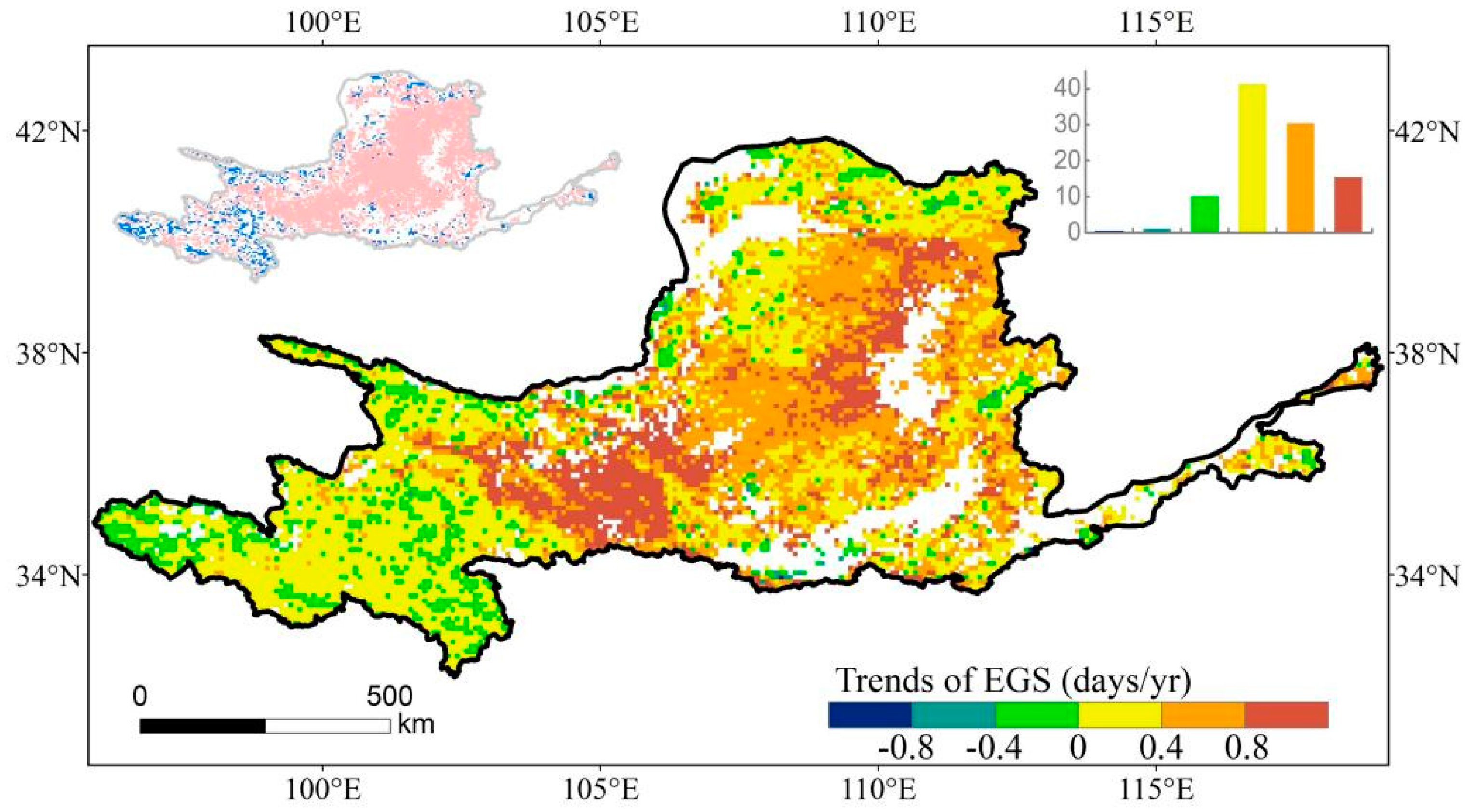
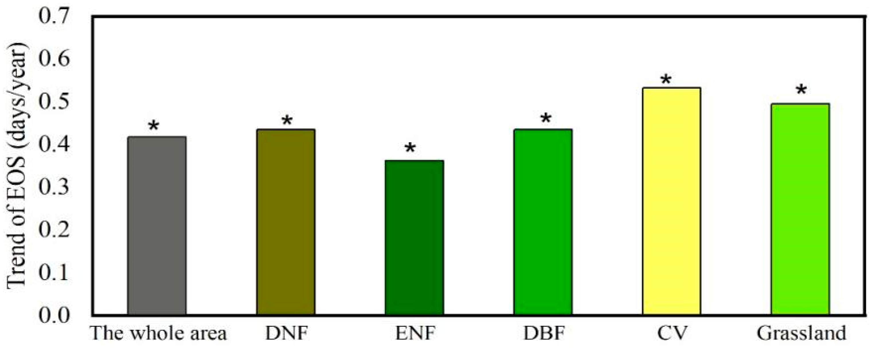
3.1. Spatio-Temporal Variations of EGS

Spatially, the postponement in EGS was observed across the majority of the YRB (89.3%) (Figure 2), and the pixels distributed in the central and western parts of the YRB showed significant delays. Conversely, a small percentage of 10.7% of the pixels exhibited an advanced trend, primarily found in the southwestern parts of the YRB. In terms of temporal changes in EGS, the YRB witnessed an annual increment in the mean delay of EGS by 0.42 days from 1982 to 2015 (Figure 3).
For different vegetation types, a uniformly significantly delayed trend in EGS was found with a range from approximately 0.37 to 0.53 days/yr. Specifically, the CV (0.53 days/yr) had the greatest delay in EGS, followed by grassland (0.50 days/yr) and DBF (0.44 days/yr).

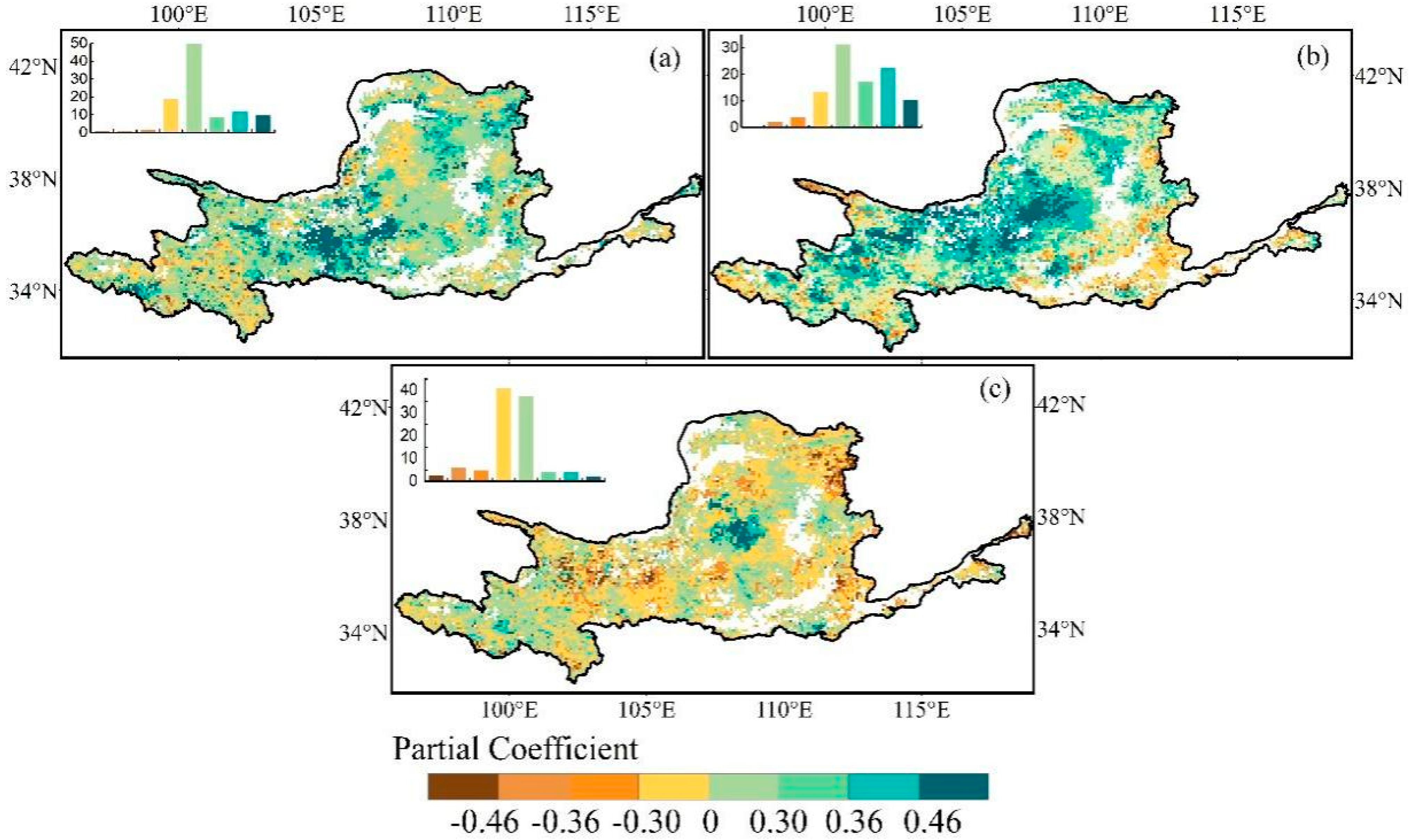
3.2. Relationships between Climatic Factors and EGS

In general, across the YRB, widespread positive correlations between EGS and preseason temperature (79.0%) and preseason precipitation (80.6%) were observed (Figure 4a,b). Specifically, in the southern region of the YRB, the preseason temperature displayed a noteworthy positive partial correlation with EGS (21.1%), whereas EGS demonstrated a concentrated positive partial correlation (32.4%) with preseason precipitation in the central areas of the YRB. Additionally, the areas where EGS was negatively correlated with preseason temperature/precipitation are concentrated in the northwestern parts and western parts, respectively. On the contrary, the spatial relationship between EGS and preseason solar radiation displayed considerable ambiguity (Figure 4c); that is, the proportion of positive (46.7%) and negative (53.3%) partial correlation coefficients was almost unanimous. The significant negative partial correlation between EGS and preseason solar radiation accounted for 8.3%, mainly distributed on the edge of the northeast of the YRB. However, EGS in the center of the YRB was significantly positively correlated with preseason solar radiation (5.2%).
For each type of vegetation, more than 70% of the pixels displayed a positive partial correlation between EGS and the preseason temperature. Out of these positive correlations, around 17% were deemed statistically significant (Figure 5). By contrast, the percentage of pixels demonstrating a notable positive partial correlation between EGS and preseason precipitation varied across different biomes. Specifically, the lowest proportion of significant positive partial correlation (1.7%) was found in the case of DNF. However, for grasslands, a much higher proportion of pixels (90.3%) displayed a positive relationship between EGS and preseason precipitation, with 36.5% of pixels being significant. Additionally, the partial correlations between EGS and preseason solar radiation were vegetation-type-dependent. Specifically, EGS was positively correlated with preseason solar radiation in DNF and DBF, whereas EGS for ENF was negatively correlated with preseason solar radiation. As for grassland and CV, the proportions of EGS negatively correlated with preseason solar radiation were 55% and 60.9%, respectively.

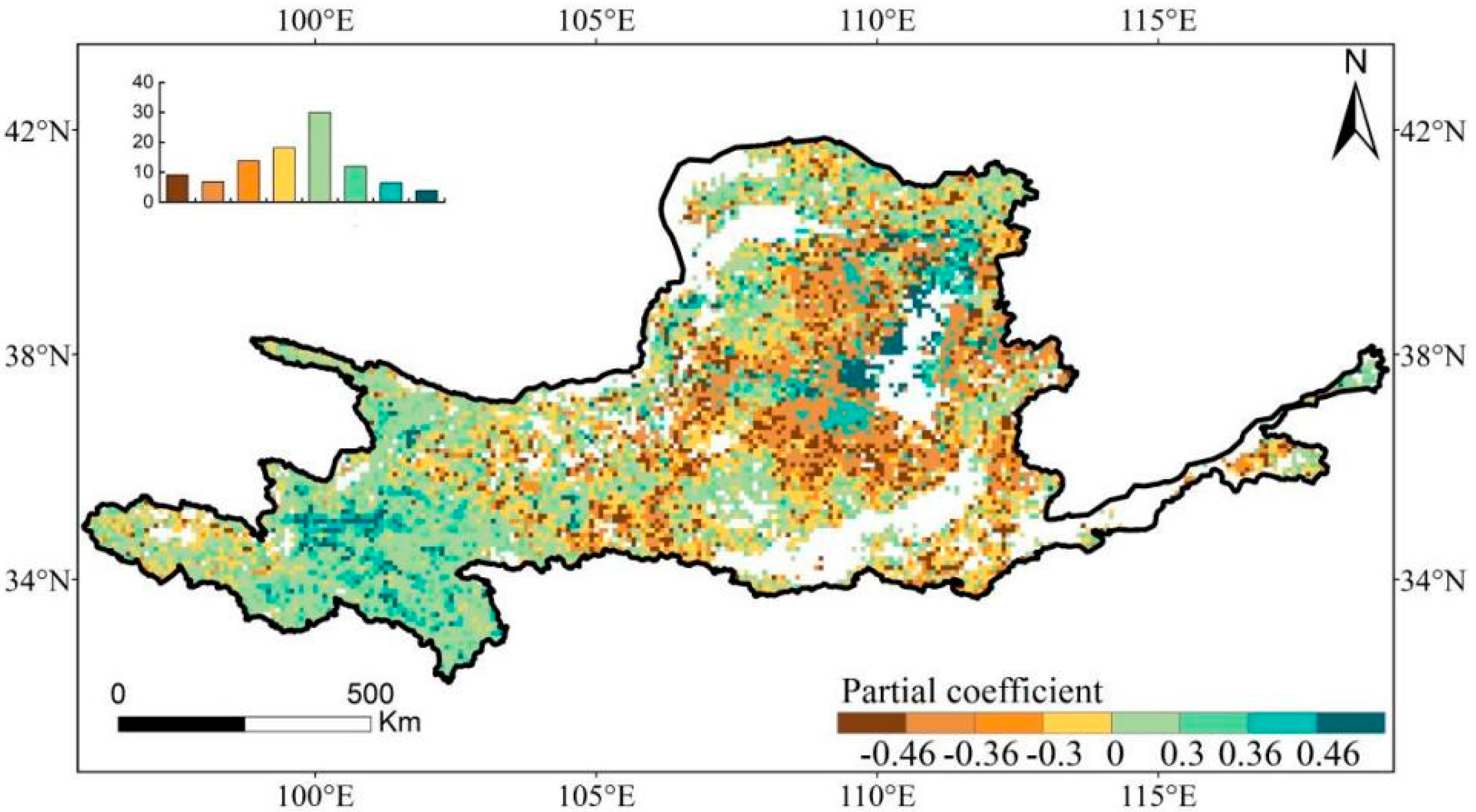
3.3. Relationships between SGS and EGS

In the western regions of the YRB, the distribution of EGS and SGS showed a positive partial correlation, which accounted for 52.1% of the pixels. Among these pixels, 10.2% exhibited statistically significant results. (Figure 6). Around 47.9% of the YRB’s central regions exhibited a negative correlation between the EGS and SGS, while approximately 15.9% of the pixels showed statistical significance.
For different biomes, SGS was positively correlated with the EGS of ENF and grassland (Figure 7) and the pixels showed a significant positive correlation of 9.2% and 12.5%, respectively. However, the EGS of other biomes had a negative correlation with SGS in more than 70% of the pixels, among which pixels with a significant negative correlation accounted for more than 20%.

3.4. Contributions of Driving Factors to the Dynamics of EGS

By utilizing GDM, the calculation for the explanatory power value of every driving factor was performed to ascertain the extent of each factor’s influence on the fluctuations of EGS over the study period (Table 1). The explanatory power value of SGS and preseason temperature was found to be the highest for the entire study area, with SGS accounting for 39.71% and preseason temperature accounting for 33.39% of the variation in EGS. This suggests that these two variables have a significant influence on the EGS. Additionally, the explanatory power of preseason precipitation was lower compared to SGS and temperature, only about 15.67%. In contrast, the preseason solar radiation had relatively less effect on the variation in EGS, with an explanatory power of 0.63%. In general, SGS exerts a substantial role in influencing the changes in EGS among driver factors.
The explanatory power of driving factors varied among different vegetation types. As far as woody plants are concerned, the explanatory power of SGS to the EGS of DBF, ENF and DNF was higher than climatic factors, which were 29.45%, 37.61% and 25.47%, respectively. Comparing the explanatory power of climatic factors for DBF, ENF and DNF, the explanatory power of solar radiation was the smallest (3.10%, 0.57% and 0.64%, respectively). The preseason temperature had the highest explanatory power for these three woody vegetation types, which reached 21.42%, 14.26% and 15.03%, respectively. One thing to note is that the explanatory power of preseason precipitation to ENF was considerably lower than that of DBF and DNF, only 5.35%. For herbaceous plants, preseason precipitation had the strongest explanatory power among all driving factors for the variation in EGS of grassland over the past 34 years, accounting for 41.61%. In contrast, the explanatory power of driving factors for CV was significantly lower than those of DBF, ENF, DNF and grassland, which means that these driving factors have limited explanatory power for the dynamic changes in the EGS of CV.

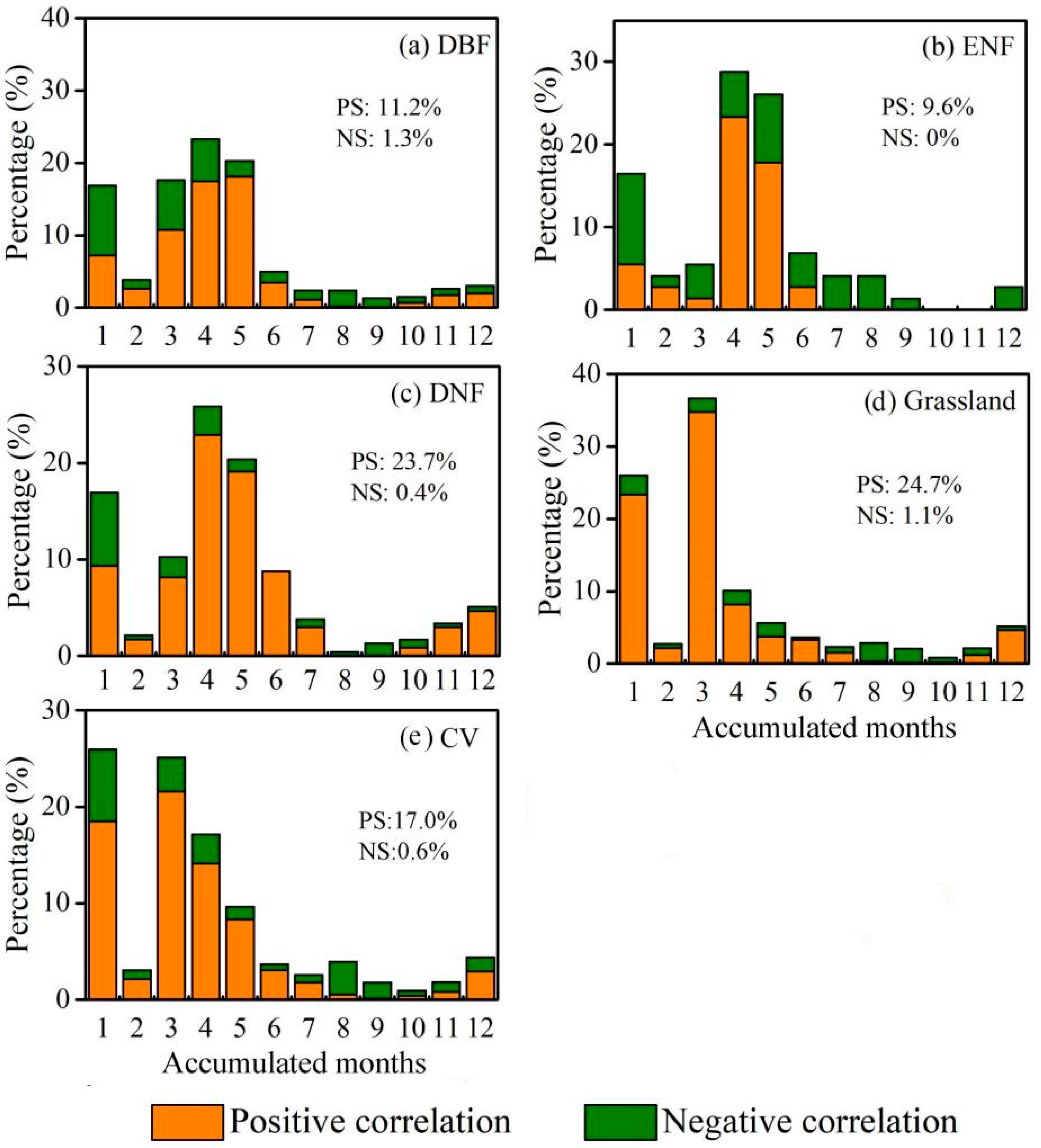
3.5. Investigating the Effect of Drought on EGS

The Rmax between EGS and SPEI reflects how the EGS responds to droughts and the accumulated months that Rmax occurred implies the sensitivity of EGS to droughts. Generally, widespread positive correlations were detected throughout the YRB (76.7%). Approximately 17.8% of pixels are statistically significant, primarily concentrated in the central areas (Figure 8). The remaining ~23.3% of all pixels located in the southern areas showed negative correlations with only 0.75% being significant. Furthermore, the accumulated months where the Rmax occurred were concentrated at 1–3 months, reaching a staggering 57.3%, which was concentrated in central and western regions. This implied that the EGS of vegetation biomes in these areas had a prompt response to drought. Additionally, approximately 28.1% of the Rmax were possessed by the 3-month SPEI, which is particularly true in the central parts. The pixels with Rmax that occurred at 4–6 months, accounting for 28.9%, were found on the edge of the eastern and western parts. Other pixels with Rmax that occurred at 7–12 months only accounted for 13.8%. These results suggested that the EGS in the YRB responded to drought at short and medium timescales.
According to the findings presented in Figure 9, the Rmax at different time scales exhibited predominantly positive values across various vegetation types. The highest percentage of maximum significant correlation was observed in grassland (25.8%), followed by DNF (24.1%) and shrub (19.8%), whereas the smallest proportion was observed in ENF (9.6%). As for the timescale of Rmax among different vegetation types, the dominant time scales for grasslands and CV seem concentrated in 1- to 4-month timescales, while the EGS of forest biomes (i.e., DBF, ENF and DNF) had slightly larger proportions with 3- to 6-month SPEI.

4. Discussion

4.1. Change in EGS across the YRB

This study reported an overall significant delayed trend in EGS of the YRB during 1982–2015, with a delaying trend of 0.42 days/yr. This delaying trend in the YRB was in accord with previous studies that investigated the variations of EGS in China based on satellite datasets provided by different sensors [13,79]. Furthermore, the delaying magnitude of EGS in our study is close to that of studies exploring a similar study area. For example, both Sun et al. [80] and Xie et al. [81] proved that EGS in the Loess Plateau region exhibited a noticeable delay trend based on the AVHRR LTDR dataset. However, the delay rate observed in the former study (0.66 days/yr) was slightly lower compared to the latter (0.74 days/yr). The slight differences among these studies are likely associated with variations in the data origins, the geographic location of the research area and the approach employed for phenology extraction. Nevertheless, as a whole, these findings suggest that our study outcomes can adequately elucidate the variations in EGS within the YRB.
Although all five types of community EGS have experienced delays over the past 34 years, there are variations in the temporal changes at the biome level. The delaying trend of cultivated vegetation was particularly prominent compared to other vegetation types. This could be attributed to the fact that cultivated vegetation is influenced not only by environmental cues but also by framing management. In certain cases, the impact of framing management outweighs that of environmental factors [82]. The delaying trend of EGS for grassland was stronger than that of woody plants (DBF/DNF/ENF) in the case of natural vegetation. This finding aligns with the results of Pei et al. [83] and Ma et al. [32], showing that the EGS of grassland on the Loess Plateau and Inner Mongolia Plateau was significantly delayed and the delaying trend was higher than that of forests and shrubs.

4.2. Regulatory Mechanisms for EGS

To evaluate the contributions of potential factors on the EGS, the GDM under the assumption of nonlinearity was implemented in this study. The results showed that among the possible driving factors, SGS has the largest explanatory power for the interannual variation in EGS at the regional scale, which is about 39.7%, followed by preseason temperature (Table 1). This indicated that SGS is the key factor governing the variations in EGS within the YRB. Previous studies undertaken in the Tibetan Plateau have likewise identified this strong control of SGS on EGS [51,84]. Additionally, the partial correlation between EGS and SGS also showed that earlier SGS might lead to earlier EGS (52.1%). This phenomenon has been extensively documented in previous studies on grasslands [13] or woody species [18] and it is predominantly connected to the self-regulation mechanism of vegetation; that is, the present phase of development shows a stronger correlation with its preceding phase [57]. Meanwhile, the adverse environmental conditions caused by changes in SGS are also considered to have an impact on EGS [85]. As proof, a colder temperature after an earlier spring budburst or an increase in pest attacks and insect outbreaks would make plants vulnerable to leaf damage [86,87]. Buermann et al. [88] suggested that soil water losses that arise from earlier SGS could increase the drought duration of summer and autumn and consequently lead to an earlier EGS. Moreover, Zu et al. [84] also suggested that there was a stronger control of SGS on EGS in harsh environments due to the circadian rhythm of vegetation. On the other hand, certain research based on experiments has put forward a fresh hypothesis suggesting that the regulation of SGS on EGS may be ascribed to a maximum limit on the storage of nonstructural carbohydrates [48,89]. It is worth noting that a notable negative relationship between EGS and SGS was also identified in a certain region of the study area. Similar reports have also been documented in the Greater Khingan Mountains and midlatitudes of the NH [52,53]. One possible explanation for this situation is that the advanced SGS and delayed EGS due to global warming from the 1980s onward [90].
For vegetation types, the explanatory power of the preseason temperature on EGS was second to SGS, especially in woody plants (DNF, DBF and ENF). The partial correlation results also showed that the EGS of woody plants had a positive correlation with the preseason temperature in more than 70% of the pixels, which indicates that the delayed EGS in woody plants might be attributed to a warmer preseason temperature. This is largely because the activity of photosynthetic enzymes of plants is controlled by temperature. The preseason temperature increase has the potential to enhance the functioning of photosynthetic enzymes, consequently retarding the breakdown of chlorophyll in the early stages of leaf senescence [91,92]. On the other hand, an increase in the preseason temperature may also lower the risk of vegetation suffering from frost damage [93]. However, the explanatory power of the preseason temperature on the variations of EGS in grasslands was weaker than that on woody plants. Furthermore, our results revealed that preseason precipitation exerts a dominant influence on the occurrence of EGS in grasslands. This phenomenon signifies that the climate and hydrothermal background in which these biomes were located contribute greatly to this occurrence. Specifically, the woody plants in the YRB were commonly distributed in the southeastern area, experiencing an annual mean precipitation ranging from 600 to 1000 mm. On the other hand, the grassland was located in the northwestern and northern areas, with annual mean precipitation between 200 and 400 mm (Figure 1c). Therefore, biomes developed distinct survival strategies for maximum adaptation to the environment [94,95]. To a certain extent, this can also explain why preseason precipitation has the largest explanatory power for the variations of EGS in grassland. Stronger control of preseason precipitation in EGS might be attributed to the intensified preseason precipitation, which potentially mitigates the adverse impacts of water stress in the autumn on plant growth, such as inhibiting photosynthesis activities and increasing the risk of chlorophyll degradation [96,97,98]. Compared to woody plants and grasslands, each driving factor (SGS, preseason temperature, preseason precipitation and preseason solar radiation) had a weak explanatory power on the variations of EGS in CV. This may be attributed to the fact that CV is more affected by human agricultural management. It was also unveiled that the preseason solar radiation had the weakest explanatory power for the interannual variations in EGS across the entire region as well as various plant species. This feeble impact of preseason insolation could plausibly be attributed to the limited sensitivity of EGS toward changes in insolation owing to abundant solar radiation in the YRB.

4.3. Autumn Phenology Response to Drought

Previous studies suggested that the timescale of the maximum correlation coefficient between vegetation indices and SPEI could help us understand how vegetation responds to drought [99,100]. Therefore, in this study, we also revolved around examining the reactions of EGS to dry-wet circumstances by using the SPEI. The results showed that drought might lead to a general advancement in the EGS across the YRB since around 76.7% of the total pixels positively correlated with SPEI. This might be related to the fact that the date of the phenology event changed since drought affected the carbon and water processes of plants [101,102]. Specifically, the preseason drought would accelerate the closing of stomata and then reduce the rate of transpiration and photosynthesis [43]. Moreover, plants need to accelerate carbon degradation to maintain respiration [103,104], thus leading to the advance of EGS. On the other hand, most studies have shown that the preceding phase’s status in the life cycle greatly influences the development and progression of the subsequent phase. Hence, the cumulative effect of water on the EGS is determined by the combined impact of water availability across different phases [79,105].
Moreover, our observations indicated that drought had a substantial cumulative impact specifically in the central region of the YRB. This impact was particularly prevalent for periods spanning 1- to 3-months and it was mainly observed in grassland. This implies that the EGS of grasslands could respond quicker to drought than other biomes. This is largely ascribed to the root functional traits and water use strategies. Although the shallow roots prevent grasslands from accessing water in deeper soil layers [106,107], the thinner roots benefit grasslands in adverse environments as they enable effective exploration of soil resources as well as decrease the reliance on symbiotic mycorrhizal fungi [108]. These two aspects together make EGS respond quickly to drought in grasslands. On the other hand, the xylem system of grasslands had a low storage capacity for water and carbon, which resulted in a lower resistance of grasslands to drought [109]. However, the timescale of Rmax for the woody plants was generally longer than herbaceous biomes, as indicated by larger proportions with 3- to 6-month SPEI. This arises from the forest biomes characterized by extensive and deeper root systems, which facilitate the absorption of water accumulated in the lower strata of the soil [110]. The thicker roots of forests also enable them to obtain abundant resources and to survive [111]. Additionally, because the water storage capacity and processes of forest biomes are more complicated than herbaceous plants [112], the EGS of forest biomes showed a tardy response when the drought occurred. Based on the varied responses of EGS among different biomes to drought, it can be concluded that grasslands were the most susceptible vegetation types to water stress. With the anticipated rise in both occurrence and severity of drought under future climate scenarios, it is suspected that grasslands that played a vital role in reducing sandstorms and preventing land degradation in the YRB would be the first to be threatened; thus, there is an urgent need to establish an accurate drought prediction system.

4.4. Uncertainties and Limitations

Although the inter-annual variation trend of EGS in the YRB obtained by using the longest time series remote sensing dataset (GIMMS NDVI3g) was consistent with previous research results, there is still a certain degree of uncertainty. The coarse spatial resolution of this dataset might result in mixed vegetation types, which consequently overlook the minor cover types and cannot capture the phenology information of all biomes [53]. Nonetheless, previous studies using GIMMS NDVI3g to investigate phenology at regional to continental scales have revealed its capacity to impart valuable insights into prolonged alterations in plant development throughout the seasons. However, increasing studies have suggested that the most effective approach to reducing uncertainty is by integrating various remote sensing datasets of differing spatial resolution to assess vegetation phenology dynamics [2]. Additionally, while GDM is important in the application in vegetation phenology studies, it is worth noting that GDM relies on clear spatial differences between geographical phenomena [113]. Large spatial scales may somewhat obscure these differences, leading to a low effect degree of the factors having microscopic spatial distribution [114]. Therefore, future research should carefully consider the sensitivity of GDM to scale.
Although the effect of several major driving factors on the EGS has been investigated, it is still unclear how the EGS responds to other factors, especially human factors. For example, land-use changes caused by large ecological engineering and urban heat island effects caused by urbanization could also result in a series of influences on the EGS [115,116]. Therefore, considering these factors in phenology studies is still a great challenge for future research.

5. Conclusions

This study focused on examining changes in the trend of EGS in various biomes within the YRB from 1982 to 2015 by using the GIMMS-3g 1/12° spatial resolution NDVI data. Additionally, correlation analysis and GDM were employed to investigate the main factors responsible for the observed alterations in EGS. Findings revealed a significant delay in the EGS for both the entire basin (0.42 days/yr) and each vegetation type. The contribution of driving factors (SGS, preseason temperature, preseason precipitation and preseason solar radiation) to the interannual variations of EGS in the YRB was detected by using the GDM. The dominant role of SGS was observed for the whole study area. For various vegetation types, the strong control of EGS in woody plants (DBF, DNF and ENF) by SGS exceeded climatic driving factors. However, for the grasslands, the predominant factor governing the fluctuations in EGS was preseason precipitation. In contrast, each driving factor has a weak explanatory power for the dynamics of EGS in CV. Additionally, the relationship between drought and EGS further proved that the EGS of grasslands was more sensitive to precipitation than that of woody plants. The findings of this investigation might assist in enhancing our comprehension of the shifts in autumn phenology within the basin ecosystem as well as how it responds to multiple driving forces.

Author Contributions

Conceptualization, M.Y.; methodology, X.L.; data curation, M.Y. and Z.W.; writing—original draft preparation, M.Y.; writing—review and editing, S.Q.; supervision, L.Z. All authors have read and agreed to the published version of the manuscript.

Funding

This research was funded by the Natural Science Foundation of Hunan Province (Grant NO. 2023JJ40226) and the Science Research Foundation of Hunan Education Bureau (Grant NO. 22B0666).

Data Availability Statement

All data needed to reach the conclusions made in this paper are presented in the paper.

Conflicts of Interest

The authors declare no conflict of interest.

References

  1. Lieth, H. Phenology and Seasonality Modeling; Springer: Berlin/Heidelberg, Germany; New York, NY, USA, 1974. [Google Scholar]
  2. Piao, S.; Liu, Q.; Chen, A.; Janssens, I.A.; Fu, Y.; Dai, J.; Zhu, X. Plant phenology and global climate change: Current progresses and challenges. Glob. Chang. Biol. 2019, 25, 1922–1940. [Google Scholar] [CrossRef] [PubMed]
  3. Richardson, A.D.; Keenan, T.F.; Migliavacca, M.; Ryu, Y.; Sonnentag, O.; Toomey, M. Climate change, phenology, and phenological control of vegetation feedbacks to the climate system. Agric. For. Meteorol. 2013, 169, 156–173. [Google Scholar] [CrossRef]
  4. Wu, C.; Gonsamo, A.; Gough, C.M.; Chen, J.M.; Xu, S. Modeling growing season phenology in north american forests using seasonal mean vegetation indices from modis. Remote Sens. Environ. 2014, 147, 79–88. [Google Scholar] [CrossRef]
  5. Cleland, E.E.; Chuine, I.; Menzel, A.; Mooney, H.A.; Schwartz, M.D. Shifting plant phenology in response to global change. Trends Ecol. Evol. 2007, 22, 357–365. [Google Scholar] [CrossRef] [PubMed]
  6. Ge, Q.; Wang, H.; Rutishauser, T.; Dai, J. Phenological response to climate change in China: A meta-analysis. Glob. Chang. Biol. 2014, 21, 265–274. [Google Scholar] [CrossRef]
  7. Fu, Y.H.; Piao, S.; Op De Beeck, M.; Cong, N.; Zhao, H.; Zhang, Y.; Janssens, I.A. Recent spring phenology shifts in western Central Europe based on multiscale observations. Glob. Ecol. Biogeogr. 2014, 23, 1255–1263. [Google Scholar] [CrossRef]
  8. Fu, Y.H.; Zhao, H.; Piao, S.; Peaucelle, M.; Peng, S.; Zhou, G.; Janssens, I.A. Declining global warming effects on the phenology of spring leaf unfolding. Nature 2015, 526, 104–107. [Google Scholar] [CrossRef]
  9. Zhang, J.; Chen, S.; Wu, Z.; Fu, Y.H. Review of vegetation phenology trends in China in a changing climate. Prog. Phys. Geogr. 2022, 46, 829–845. [Google Scholar] [CrossRef]
  10. Zhu, W.; Tian, H.; Xu, X.; Pan, Y.; Chen, G.; Lin, W. Extension of the growing season due to delayed autumn over mid and high latitudes in North America during 1982–2006. Glob. Ecol. Biogeogr. 2012, 21, 260–271. [Google Scholar] [CrossRef]
  11. Zhou, L.; Tucker, C.J.; Kaufmann, R.K.; Slayback, D.; Shabanov, N.V.; Myneni, R.B. Variations in northern vegetation activity inferred from satellite data of vegetation index during 1981 to 1999. J. Geophys. Res. Atmos. 2001, 1984–2012, 20069–20083. [Google Scholar] [CrossRef]
  12. Liu, Q.; Fu, Y.H.; Zeng, Z.; Huang, M.; Li, X.; Piao, S. Temperature, precipitation, and insolation effects on autumn vegetation phenology in temperate China. Glob. Chang. Biol. 2016, 22, 644–656. [Google Scholar] [CrossRef] [PubMed]
  13. Liu, Q.; Fu, Y.H.; Zhu, Z.; Liu, Y.; Liu, Z.; Huang, M.; Janssens, I.A.; Piao, S. Delayed autumn phenology in the Northern Hemisphere is related to change in both climate and spring phenology. Glob. Chang. Biol. 2016, 22, 3702–3711. [Google Scholar] [CrossRef] [PubMed]
  14. Gao, X.; Zhao, D. Impacts of climate change on vegetation phenology over the Great Lakes Region of Central Asia from 1982 to 2014. Sci. Total Environ. 2022, 845, 157227. [Google Scholar] [CrossRef]
  15. Yuan, H.; Wu, C.; Gu, C.; Wang, X. Evidence for satellite observed changes in the relative influence of climate indicators on autumn phenology over the Northern Hemisphere. Glob. Planet. Chang. 2020, 187, 103131. [Google Scholar] [CrossRef]
  16. Bao, G.; Jin, H.; Tong, S.; Chen, J.; Huang, X.; Bao, Y.; Shao, C.; Mandakh, U.; Chopping, M.; Du, L. Autumn phenology and its covariation with climate, spring phenology and annual peak growth on the mongolian plateau. Agric. For. Meteorol. 2021, 298–299, 108312. [Google Scholar] [CrossRef]
  17. Wang, X.; Xiao, J.; Li, X.; Cheng, G.; Ma, M.; Zhu, G.; Arain, M.A.; Black, T.A.; Jassal, R.S. No trends in spring and autumn phenology during the global warming hiatus. Nat. Commun. 2019, 10, 2389. [Google Scholar] [CrossRef]
  18. Keenan, T.F.; Richardson, A.D. The timing of autumn senescence is affected by the time of spring phenology: Implications for predictive models. Glob. Chang. Biol. 2015, 21, 2634–2641. [Google Scholar] [CrossRef]
  19. Gallinat, A.S.; Primack, R.B.; Wagner, D.L. Autumn, the neglected season in climate change research. Trends Ecol. Evol. 2015, 30, 169–176. [Google Scholar] [CrossRef]
  20. Wu, C.Y.; Chen, J.M.; Black, T.A. Interannual variability of net ecosystem productivity in forests is explained by carbon flux phenology in autumn. Glob. Ecol. Biogeogr. 2013, 22, 994–1006. [Google Scholar] [CrossRef]
  21. Zhang, J.; Xiao, J.; Tong, X. NIRv and SIF better estimate phenology than NDVI and EVI: Effects of spring and autumn phenology on ecosystem production of planted forests. Agric. For. Meteoro. 2022, 315, 108819. [Google Scholar] [CrossRef]
  22. Zohner, C.M.; Rockinger, A.; Renner, S.S. Increased autumn productivity permits temperate trees to compensate for spring frost damage. New Phytol. 2019, 221, 789–795. [Google Scholar] [CrossRef]
  23. Cooke, J.E.; Eriksson, M.E.; Junttila, O. The dynamic nature of bud dormancy in trees: Environmental control and molecular mechanisms. Plant Cell Environ. 2012, 35, 1707–1728. [Google Scholar] [CrossRef]
  24. Soolanayakanahally, R.Y.; Guy, R.D.; Silim, S.N. Timing of photoperiodic competency causes phenological mismatch in balsam poplar (Populus balsamifera L.). Plant Cell Environ. 2012, 36, 116–127. [Google Scholar] [CrossRef]
  25. Flynn, D.F.B.; Wolkovich, E.M. Temperature and photoperiod drive spring phenology across all species in a temperate forest community. New Phytol. 2018, 219, 1353–1362. [Google Scholar] [CrossRef] [PubMed]
  26. Xie, Y.; Wang, X.; Silander, J.A. Deciduous forest responses to temperature, precipitation, and drought imply complex climate change impacts. Proc. Natl. Acad. Sci. USA 2015, 112, 13585–13590. [Google Scholar] [CrossRef] [PubMed]
  27. Worrall, J. Autumn leaf colouration. For. Chron. 1998, 74, 668–669. [Google Scholar]
  28. Lang, W.; Chen, X.; Qian, S. A new process-based model for predicting autumn phenology: How is leaf senescence controlled by photoperiod and temperature coupling? Agric. For. Meteoro. 2019, 268, 124–135. [Google Scholar] [CrossRef]
  29. Liu, Q.; Piao, S.L.; Fu, Y.S.H.; Gao, M.D.; Penuelas, J.; Janssens, I.A. Climatic warming increases spatial synchrony in spring vegetation phenology across the Northern Hemisphere. Geophys. Res. Lett. 2019, 46, 1641–1650. [Google Scholar] [CrossRef]
  30. Guo, M.; Wu, C.; Peng, J. Identifying contributions of climatic and atmospheric changes to autumn phenology over mid-high latitudes of Northern Hemisphere. Glob. Planet. Chang. 2021, 197, 103396. [Google Scholar] [CrossRef]
  31. Dragoni, D.; Rahman, A.F. Trends in fall phenology across the deciduous forests of the Eastern USA. Agric. For. Meteorol. 2012, 157, 96–105. [Google Scholar] [CrossRef]
  32. Ma, R.; Shen, X.J.; Zhang, J.Q.; Xia, C.L. Variation of vegetation autumn phenology and its climatic drivers in temperate grasslands of China. Int. J. Appl. Earth Obs. 2022, 114, 103064. [Google Scholar] [CrossRef]
  33. Ren, P.; Liu, Z.; Zhou, X.; Peng, C.P.; Xiao, J.; Wang, S. Strong controls of daily minimum temperature on the autumn photosynthetic phenology of subtropical vegetation in China. For. Ecosyst. 2021, 8, 31. [Google Scholar] [CrossRef]
  34. Ren, S.; Vitasse, Y.; Chen, X.; Peichl, M.; An, S. Assessing the relative importance of sunshine, temperature, precipitation, and spring phenology in regulating leaf senescence timing of herbaceous species in China. Agric. For. Meteorol. 2022, 313, 108770. [Google Scholar] [CrossRef]
  35. Estiarte, M.; Peñuelas, J. Alteration of the phenology of leaf senescence and fall in winter deciduous species by climate change: Effects on nutrient proficiency. Glob. Chang. Biol. 2015, 21, 1005–1017. [Google Scholar] [CrossRef]
  36. Hänninen, H. Boreal and Temperate Trees in a Changing Climate (Biometeorology); Springer: Dordrecht, The Netherlands, 2016. [Google Scholar]
  37. Zhang, R.; Qi, J.; Leng, S.; Wang, Q. Long-Term Vegetation Phenology Changes and Responses to Preseason Temperature and Precipitation in Northern China. Remote Sens. 2022, 14, 1396. [Google Scholar] [CrossRef]
  38. Wu, C.; Peng, J.; Ciais, P.; Peñuelas, J.; Wang, H.; Beguería, S.; Ge, Q. Increased drought effects on the phenology of autumn leaf senescence. Nat. Clim. Chang. 2022, 12, 943–949. [Google Scholar] [CrossRef]
  39. Du, P.; Arndt, S.K.; Farrell, C. Is plant survival on green roofs related to their drought response, water use or climate of origin? Sci. Total Environ. 2019, 667, 25–32. [Google Scholar] [CrossRef]
  40. Zhao, J.; Huang, S.; Huang, Q.; Wang, H.; Leng, G.; Fang, W. Time-lagged response of vegetation dynamics to climatic and teleconnection factors. Catena 2020, 189, 104474. [Google Scholar] [CrossRef]
  41. Wei, X.; He, W.; Zhou, Y.; Cheng, N.; Ju, W. Increased sensitivity of global vegetation productivity to drought over the recent three decades. J. Geophys. Res.-Atmos. 2023, 128, e2022JD037504. [Google Scholar] [CrossRef]
  42. Cui, T.; Martz, L.; Guo, X. Grassland phenology response to drought in the Canadian Prairies. Remote Sens. 2017, 9, 1258. [Google Scholar] [CrossRef]
  43. Kang, W.; Wang, T.; Liu, S. The response of vegetation phenology and productivity to drought in semi-arid regions of Northern China. Remote Sens. 2018, 10, 727. [Google Scholar] [CrossRef]
  44. Xie, Y.; Wang, X.; Wilson, A.M., Jr.; Silander, J.A. Predicting autumn phenology: How deciduous tree species respond to weather stressors. Agric. For. Meteorol. 2018, 250–251, 127–137. [Google Scholar] [CrossRef]
  45. Yuan, Z.; Tong, S.; Bao, G. Spatiotemporal variation of autumn phenology responses to preseason drought and temperature in alpine and temperate grasslands in China. Sci. Total Environ. 2023, 859, 160373. [Google Scholar] [CrossRef] [PubMed]
  46. Ge, C.H.; Sun, S.; Yao, R.; Sun, P.; Li, M.; Bian, Y.J. Long-term vegetation phenology changes and response to multi-scale meteorological drought on the Loess Plateau, China. J. Hydrol. 2022, 614, 128605. [Google Scholar] [CrossRef]
  47. Huang, L.; He, B.; Han, L.; Liu, J.; Wang, H.; Chen, Z. A global examination of the response of ecosystem water-use efficiency to drought based on MODIS data. Sci. Total Environ. 2017, 601–602, 1097–1107. [Google Scholar] [CrossRef]
  48. Fu, Y.S.; Campioli, M.; Vitasse, Y.; De Boeck, H.J.; Van den Berge, J.; AbdElgawad, H.; Janssens, I.A. Variation in leaf flushing date influences autumnal senescence and next year’s flushing date in two temperate tree species. Proc. Natl. Acad. Sci. USA 2014, 111, 7355–7360. [Google Scholar] [CrossRef]
  49. Wu, C.; Hou, X.; Peng, D.; Gonsamo, A.; Xu, S. Land surface phenology of China’s temperate ecosystems over 1999–2013: Spatial–temporal patterns, interaction effects, covariation with climate and implications for productivity. Agric. For. Meteorol. 2016, 216, 177–187. [Google Scholar] [CrossRef]
  50. Zani, D.; Crowther, T.W.; Mo, L.; Renner, S.S.; Zohner, C.M. Increased growingseason productivity drives earlier autumn leaf senescence in temperate trees. Science 2020, 370, 1066–1071. [Google Scholar] [CrossRef]
  51. Peng, J.; Wu, C.; Wang, X.; Lu, L. Spring phenology outweighed climate change in determining autumn phenology on the Tibetan Plateau. Int. J. Climatol. 2021, 41, 3725–3742. [Google Scholar] [CrossRef]
  52. Ren, M. Peichl, Enhanced spatiotemporal heterogeneity and the climatic and biotic controls of autumn phenology in northern grasslands. Sci. Total Environ. 2021, 788, 147806. [Google Scholar] [CrossRef]
  53. Fu, Y.; He, H.S.; Zhao, J.; Larsen, D.R.; Zhang, H.; Sunde, M.G.; Duan, S. Climate and Spring Phenology Effects on Autumn Phenology in the Greater Khingan Mountains, Northeastern China. Remote Sens. 2018, 10, 449. [Google Scholar] [CrossRef]
  54. Gao, X.; Dai, J.; Tao, Z.; Shahzad, K.; Wang, H. Autumn phenology of tree species in China is associated more with climate than with spring phenology and phylogeny. Front. Plant Sci. 2023, 14, 1040758. [Google Scholar] [CrossRef] [PubMed]
  55. He, Z.; Du, J.; Zhao, W.; Yang, J.; Chen, L.; Zhu, X.; Chang, X.; Liu, H. Assessing temperature sensitivity of subalpine shrub phenology in semi-arid mountain regions of China. Agric. For. Meteorol. 2015, 213, 42–52. [Google Scholar] [CrossRef]
  56. Du, J.; He, Z.; Piatek, K.B.; Chen, L.; Lin, P.; Zhu, X. Interacting effects of temperature and precipitation on climatic sensitivity of spring vegetation green-up in arid mountains of China. Agric. For. Meteorol. 2019, 269, 71–77. [Google Scholar] [CrossRef]
  57. Zhao, W.; Hu, Z.; Guo, Q.; Wu, G.; Chen, R.; Li, S. Contributions of climatic factors to interannual variability of the vegetation index in northern china grasslands. J. Clim. 2020, 33, 175–183. [Google Scholar] [CrossRef]
  58. Liang, K.; Liu, S.; Bai, P.; Nie, R. The Yellow River basin becomes wetter or drier? The case as indicated by mean precipitation and extremes during 1961–2012. Theor. Appl. Climatol. 2015, 119, 701–722. [Google Scholar] [CrossRef]
  59. Tian, Q.; Yang, S. Regional climatic response to global warming: Trends in temperature and precipitation in the Yellow, Yangtze and Pearl River basins since the 1950s. Quatern. Int. 2017, 440, 1–11. [Google Scholar] [CrossRef]
  60. She, D.; Xia, J. The spatial and temporal analysis of dry spells in the Yellow River basin, China. Stoch. Environ. Res. Risk. Assess. 2013, 27, 29–42. [Google Scholar] [CrossRef]
  61. Wang, Y.; Luo, Y.; Shafeeque, M. Interpretation of vegetation phenology changes using daytime and night-time temperatures across the Yellow River Basin, China. Sci. Total Environ. 2019, 693, 133553. [Google Scholar] [CrossRef]
  62. Yuan, M.; Zhao, L.; Lin, A.; Li, Q.; She, D.; Qu, S. How do climatic and non-climatic factors contribute to the dynamics of vegetation autumn phenology in the Yellow River Basin, China? Ecol. Indic. 2020, 112, 106112. [Google Scholar] [CrossRef]
  63. Pinzon, J.; Tucker, C. A non-stationary 1981–2012 AVHRR NDVI3g time series. Remote Sens. 2014, 6, 6929–6960. [Google Scholar] [CrossRef]
  64. Chen, Y.Y.; Yang, K.; He, J.; Qin, J.; Shi, J.C.; Du, J.Y.; He, Q. Improving land surface temperature modeling for dry land of China. J. Geophys. Res. 2011, 116, D20104. [Google Scholar] [CrossRef]
  65. Vicente-Serrano, S.M.; Beguería, S.; López-Moreno, J.I. A multiscalar drought index sensitive to global warming: The standardized precipitation evapotranspiration index. J. Clim. 2010, 23, 1696–1718. [Google Scholar] [CrossRef]
  66. Li, P.; Liu, Z.; Zhou, X.; Li, Z.; Luo, Y.; Peng, C. Combined control of multiple extreme climate stressors on autumn vegetation phenology on the Tibetan Plateau under past and future climate change. Agric. For. Meteorol. 2021, 308, 108571. [Google Scholar] [CrossRef]
  67. Cong, N.; Wang, T.; Nan, H.; Ma, Y.; Wang, X.; Myneni, R.B.; Piao, S. Changes in satellite-derived spring vegetation green-up date and its linkage to climate in China from 1982 to 2010: A multimethod analysis. Glob. Chang. Biol. 2013, 19, 881–891. [Google Scholar] [CrossRef]
  68. Liu, Z.; Wu, C.; Liu, Y.; Wang, X.; Fang, B.; Yuan, W.; Ge, Q. Spring green-up date derived from GIMMS3g and SPOT-VGT NDVI of winter wheat cropland in the North China Plain. ISPRS J. Photogramm. 2017, 130, 81–91. [Google Scholar] [CrossRef]
  69. Piao, S.; Fang, J.Y.; Zhou, L.M.; Ciais, P.; Zhu, B. Variations in satellite-derived phenology in China’s temperate vegetation. Glob. Chang. Biol. 2006, 12, 672–685. [Google Scholar] [CrossRef]
  70. Gocic, M.; Trajkovic, S. Analysis of changes in meteorological variables using Mann-Kendall and Sen’s slope estimator statistical tests in Serbia. Glob. Planet. Chang. 2013, 100, 172–182. [Google Scholar] [CrossRef]
  71. Wang, G.; Luo, Z.; Huang, Y.; Wei, Y.; Lin, X.; Sun, W. Preseason heat requirement and days of precipitation jointly regulate plant phenological variations in Inner Mongolian grassland. Agric. For. Meteorol. 2022, 314, 108783. [Google Scholar] [CrossRef]
  72. Yu, F.; Price, K.P.; Ellis, J.; Shi, P. Response of seasonal vegetation development to climatic variations in eastern central Asia. Remote Sens. Environ. 2003, 87, 42–54. [Google Scholar] [CrossRef]
  73. Wu, C.; Wang, X.; Wang, H.; Ciais, P.; Peñuelas, J.; Myneni, R.B.; Jassal, R.S. Contrasting responses of autumn-leaf senescence to daytime and night-time warming. Nat. Clim. Chang. 2018, 8, 1092. [Google Scholar] [CrossRef]
  74. Wang, M.; Li, P.; Peng, C.; Zhou, X.; Luo, Y.; Zhang, C. Divergent responses of autumn vegetation phenology to climate extremes over northern middle and high latitudes. Glob. Ecol. Biogeogr. 2022, 31, 2281–2296. [Google Scholar] [CrossRef]
  75. Wang, J.F.; Li, X.H.; Christakos, G.; Liao, Y.L.; Zhang, T.; Gu, X.; Zheng, X.Y. Geographical detectors–based health risk assessment and its application in the neural tube defects study of the Heshun Region, China. Int. J. Geogr. Inf. Sci. 2010, 24, 107–127. [Google Scholar] [CrossRef]
  76. Peng, W.; Kuang, T.; Tao, S. Quantifying influences of natural factors on vegetation NDVI changes based on geographical detector in Sichuan, western China. J. Clean. Prod. 2019, 233, 353–367. [Google Scholar] [CrossRef]
  77. Zhao, W.; Yu, X.; Jiao, C.; Xu, C.; Liu, Y.; Wu, G. Increased association between climate change and vegetation index variation promotes the coupling of dominant factors and vegetation growth. Sci. Total Environ. 2021, 767, 144669. [Google Scholar] [CrossRef] [PubMed]
  78. Peng, J.; Wu, C.; Zhang, X.; Wang, X.; Gonsamo, A. Satellite detection of cumulative and lagged effects of drought on autumn leaf senescence over the Northern Hemisphere. Glob. Chang. Biol. 2019, 25, 2174–2188. [Google Scholar] [CrossRef]
  79. Yang, Y.; Guan, H.; Shen, M.; Liang, W.; Jiang, L. Changes in autumn vegetation dormancy onset date and the climate controls across temperate ecosystems in china from 1982 to 2010. Glob. Chang. Biol. 2015, 21, 652–665. [Google Scholar] [CrossRef]
  80. Sun, W.; Song, X.; Mu, X.; Gao, P.; Wang, F.; Zhao, G. Spatiotemporal vegetation cover variations associated with climate change and ecological restoration in the Loess Plateau. Agric. For. Meteorol. 2015, 209, 87–99. [Google Scholar] [CrossRef]
  81. Xie, B.; Qin, Z.; Wang, Y.; Chang, Q. Monitoring vegetation phenology and their response to climate change on Chinese Loess Plateau based on remote sensing. Trans. Chin. Soc. Agric. Eng. 2015, 31, 153–160. [Google Scholar]
  82. Liu, Y.; Chen, Q.; Ge, Q.; Dai, J.; Qin, Y.; Dai, L.; Chen, J. Modelling the impacts of climate change and crop management on phenological trends of spring and winter wheat in China. Agric. For. Meteorol. 2018, 248, 518–526. [Google Scholar] [CrossRef]
  83. Pei, T.; Ji, Z.; Chen, Y.; Wu, H.; Hou, Q.; Qin, G.; Xie, B. The sensitivity of vegetation phenology to extreme climate indices in the Loess Plateau, China. Sustainability 2021, 13, 7623. [Google Scholar] [CrossRef]
  84. Zu, J.; Zhang, Y.; Huang, K.; Liu, Y.; Chen, N.; Cong, N. Biological and climate factors co-regulated spatial-temporal dynamics of vegetation autumn phenology on the Tibetan Plateau. Int. J. Appl. Earth Obs. 2018, 69, 198–205. [Google Scholar] [CrossRef]
  85. Cong, N.; Shen, M.G.; Piao, S.L. Spatial variations in responses of vegetation autumn phenology to climate change on the Tibetan Plateau. J. Plant. Ecol. 2017, 10, 744–752. [Google Scholar] [CrossRef]
  86. Hufkens, K.; Friedl, M.A.; Keenan, T.F.; Sonnentag, O.; Bailey, A.; O’keefe, J.; Richardson, A.D. Ecological impacts of a widespread frost event following early spring leaf–out. Glob. Chang. Biol. 2012, 18, 2365–2377. [Google Scholar] [CrossRef]
  87. Jepsen, J.U.; Kapari, L.; Hagen, S.B.; Schott, T.; Vindstad, O.P.L.; Nilssen, A.C.; Ims, R.A. Rapid northwards expansion of a forest insect pest attributed to spring phenology matching with sub-Arctic birch. Glob. Chang. Biol. 2011, 17, 2071–2083. [Google Scholar] [CrossRef]
  88. Buermann, W.; Bikash, P.R.; Jung, M.; Burn, D.H.; Reichstein, M. Earlier springs decrease peak summer productivity in North American boreal forests. Environ. Res. Lett. 2013, 8, 024027. [Google Scholar] [CrossRef]
  89. Fatichi, S.; Leuzinger, S.; Körner, C. Moving beyond photosynthesis: From carbon source to sink-driven vegetation modeling. New Phytol. 2014, 201, 1086–1095. [Google Scholar] [CrossRef] [PubMed]
  90. Jeong, S.J.; Ho, C.H.; Gim, H.J.; Brown, M.E. Phenology shifts at start vs. end of growing season in temperate vegetation over the Northern Hemisphere for the period 1982–2008. Glob. Chang. Biol. 2011, 17, 2385–2399. [Google Scholar] [CrossRef]
  91. Shi, C.; Sun, G.; Zhang, H.; Xiao, B.; Ze, B.; Zhang, N.; Wu, N. Effects of warming on chlorophyll degradation and carbohydrate accumulation of Alpine herbaceous species during plant senescence on the Tibetan Plateau. PLoS ONE 2014, 9, e107874. [Google Scholar] [CrossRef] [PubMed]
  92. Fracheboud, Y.; Luquez, V.; Bjorken, L.; Sjodin, A.; Tuominen, H.; Jansson, S. The control of autumn senescence in European aspen. Plant. Physiol. 2009, 149, 1982–1991. [Google Scholar] [CrossRef]
  93. Hartmann, D.; Klein, T.A.; Rusicucci, M. Observations: Atmosphere and surface. In Climate Change 2013: The Physical Science Basis. Contribution of Working Group I to the Fifth Assessment Report of the Intergovernmental Panel on Climate Change; Cambridge University Press: Cambridge, UK; New York, NY, USA, 2013; pp. 159–254. [Google Scholar]
  94. Farre, E.M. The regulation of plant growth by the circadian clock. Plant Biol. 2012, 14, 401–410. [Google Scholar] [CrossRef] [PubMed]
  95. Sultan, S.E. Phenotypic plasticity for plant development, function and life history. Trends Plant Sci. 2000, 5, 537–542. [Google Scholar] [CrossRef] [PubMed]
  96. Tezara, W.; Mitchell, V.; Driscoll, S.; Lawlor, D. Water stress inhibits plant photosynthesis by decreasing coupling factor and ATP. Nature 1999, 401, 914–917. [Google Scholar] [CrossRef]
  97. Anderegg, W.R.; Plavcov, A.L.; Anderegg, L.D.; Hacke, U.G.; Berry, J.A.; Field, C.B. Drought’s legacy: Multiyear hydraulic deterioration underlies widespread aspen forest die-off and portends increased future risk. Glob. Chang. Biol. 2013, 19, 1188–1196. [Google Scholar] [CrossRef]
  98. Dreesen, F.; De Boeck, H.; Janssens, I.; Nijs, I. Do successive climate extremes weaken the resistance of plant communities? An experimental study using plant assemblages. Biogeosciences 2014, 11, 109–121. [Google Scholar] [CrossRef]
  99. Vicente-Serrano, S.M.; Gouveia, C.; Camarero, J.J.; Beguería, S.; Trigo, R.; López-Moreno, J.I.; Morán-Tejeda, E. Response of vegetation to drought time-scales across global land biomes. Proc. Natl. Acad. Sci. USA 2013, 110, 52–57. [Google Scholar] [CrossRef]
  100. Xu, H.J.; Wang, X.P.; Zhao, C.Y.; Yang, X.M. Diverse responses of vegetation growth to meteorological drought across climate zones and land biomes in northern China from 1981 to 2014. Agric. For. Meteorol. 2018, 262, 1–13. [Google Scholar] [CrossRef]
  101. Zhao, M.; Running, S.W. Drought-induced reduction in global terrestrial net primary production from 2000 through 2009. Science 2010, 329, 940–943. [Google Scholar] [CrossRef]
  102. Van der Molen, M.K.; Dolman, A.J.; Ciais, P.; Eglin, T.; Gobron, N.; Law, B.E.; Meir, P.; Peters, W.; Phillips, O.L.; Reichstein, M. Drought and ecosystem carbon cycling. Agric. For. Meteorol. 2011, 151, 765–773. [Google Scholar] [CrossRef]
  103. Xu, Z.; Zhou, G.; Shimizu, H. Plant responses to drought and rewatering. Plant Signal. Behav. 2010, 5, 649–654. [Google Scholar] [CrossRef]
  104. Chapin, F.S., III; Matson, P.A.; Vitousek, P. Principles of Terrestrial Ecosystem Ecology; Springer Science & Business Media: Berlin, Germany, 2011. [Google Scholar]
  105. Ma, X.; Huete, A.; Moran, S.; Ponce-Campos, G.; Eamus, D. Abrupt shifts in phenology and vegetation productivity under climate extremes. J. Geophys. Res. Biogeo. 2015, 120, 2036–2052. [Google Scholar] [CrossRef]
  106. Dorji, T.; Totland, O.; Moe, S.R.; Hopping, K.A.; Pan, J.B.; Klein, J.A. Plant functional traits mediate reproductive phenology and success in response to experimental warming and snow addition in Tibet. Glob. Chang. Biol. 2013, 19, 459–472. [Google Scholar] [CrossRef] [PubMed]
  107. Fan, Y.; Miguez-Macho, G.; Jobbágy, E.G.; Jackson, R.B.; OteroCasal, C. Hydrologic regulation of plant rooting depth. Proc. Natl. Acad. Sci. USA 2017, 114, 10572–10577. [Google Scholar] [CrossRef] [PubMed]
  108. Knapp, A.K.; Carroll, C.J.W.; Denton, E.M.; La Pierre, K.J.; Collins, S.L.; Smith, M.D. Differential sensitivity to regional-scale drought in six central US grasslands. Oecologia 2015, 177, 949–957. [Google Scholar] [CrossRef]
  109. Craine, J.M.; Ocheltree, T.W.; Nippert, J.B.; Towne, E.G.; Skibbe, A.M.; Kembel, S.W.; Fargione, J.E. Global diversity of drought tolerance and grassland climatechange resilience. Nat. Clim. Chang. 2013, 3, 63–67. [Google Scholar] [CrossRef]
  110. Davidson, E.A.; Verchot, L.V.; Cattanio, J.H.; Ackerman, I.L.; Carvalho, J.E.M. Effects of soil water content on soil respiration in forests and cattle pastures of eastern Amazonia. Biogeochemistry 2000, 48, 53–69. [Google Scholar] [CrossRef]
  111. Ma, Z.; Guo, D.; Xu, X.; Lu, M.; Bardgett, R.D.; Eissenstat, D.M.; Hedin, L.O. Evolutionary history resolves global organization of root functional traits. Nature 2018, 555, 94–97. [Google Scholar] [CrossRef]
  112. Tian, F.; Wigneron, J.P.; Ciais, P.; Chave, J.; Ogee, J.; Penuelas, J.; Fensholt, R. Coupling of ecosystem-scale plant water storage and leaf phenology observed by satellite. Nat. Ecol. Evol. 2018, 2, 1428–1435. [Google Scholar] [CrossRef]
  113. Wang, J.; Zhang, T.; Fu, B. A measure of spatial stratified heterogeneity. Ecol. Indic. 2016, 67, 250–256. [Google Scholar] [CrossRef]
  114. Zhao, Y.; Liu, L.; Kang, S.; Ao, Y.; Han, L.; Ma, C. Quantitative analysis of factors influencing spatial distribution of soil erosion based on geo-detector model under diverse geomorphological types. Land 2021, 10, 604. [Google Scholar] [CrossRef]
  115. Zhou, D.; Zhao, S.; Zhang, L.; Liu, S. Remotely sensed assessment of urbanization effects on vegetation phenology in China’s 32 major cities. Remote Sens. Environ. 2016, 176, 272–281. [Google Scholar] [CrossRef]
  116. Liu, Z.; Liu, Y. Does Anthropogenic Land Use Change Play a Role in Changes of Precipitation Frequency and Intensity over the Loess Plateau of China? Remote Sens. 2018, 10, 1818. [Google Scholar] [CrossRef]
Figure 1. Location of the YRB (a) and spatial pattern of mean air temperature (b), average annual precipitation (c).
Remotesensing 15 05058 g001
Figure 2. Spatial distribution of the linear trend of EGS. Top-left inset illustrates the significance of the trend (pink denotes statistical significance at a 95% confidence level). Top-right inset plot shows the frequency distribution of EGS.
Remotesensing 15 05058 g002
Figure 3. Average linear trend and standard deviation of EGS in different vegetation types across the YRB from 1982 to 2015. * indicates statistical significance at a 95% confidence level.
Remotesensing 15 05058 g003
Figure 4. Spatial distribution of partial correlation coefficients between EGS and preseason temperature (a); preseason precipitation (b); and preseason solar radiation (c) in the YRB. Coefficient values of ±0.46 and ±0.36 are indicated at the 99% and 95% significance levels, respectively. Top-left insets represent the frequency distributions of the corresponding coefficients of which the values were indicated by the map legend.
Remotesensing 15 05058 g004
Figure 5. The frequency distribution of partial correlation coefficients between EGS and climatic factors for each vegetation type in the YRB: (a) deciduous coniferous forest; (b) evergreen coniferous forest; (c) deciduous broad-leaved forest; (d) grassland; (e) cultivated vegetation. Blue, red and yellow represent the frequency distribution of partial correlation coefficients between EGS and preseason precipitation, preseason temperature and preseason solar radiation, respectively. Texts in each subfigure present the percentage of partial correlations between EGS and preseason temperature, precipitation and solar radiation. P indicates a positive correlation, N indicates a negative correlation, the ratio in parentheses indicates the percentage of pixels at the 95% level of significance level.
Remotesensing 15 05058 g005
Figure 6. Spatial distribution of partial correlation coefficients between EGS and SGS in the YRB during 1982–2015. Coefficient values of ±0.46 and ±0.36 are indicated at the 99% and 95% significance levels, respectively. The top-left inset represents the frequency distributions of the corresponding coefficients, of which the values were indicated by the map legend.
Remotesensing 15 05058 g006
Figure 7. Percentages of the partial correlation coefficient between EGS and SGS of different vegetation types from 1982 to 2015. Bars above 0 and below 0 represent the percentage of positive and negative correlations, respectively. Colored sections indicate the percentage of correlations that are statistically significant at the 95% level.
Remotesensing 15 05058 g007
Figure 8. Spatial distribution of the maximum partial correlation coefficient between EGS and SPEI from 1982 to 2015 (a) and the corresponding time scales at which maximum partial correlation coefficient occurred are obtained (b). Coefficient values of ±0.46 and ±0.36 are indicated at the 99% and 95% significance levels, respectively.
Remotesensing 15 05058 g008
Figure 9. Percentage of the Rmax between EGS and SPEI at different time scales (1- to 12-month) for each vegetation type: (a) deciduous coniferous forest; (b) evergreen coniferous forest; (c) deciduous broad-leaved forest; (d) grassland; (e) cultivated vegetation. Note: PS represents the ratio of pixels having a significant positive correlation between EGS and SPEI on a 1- to 12-month time scale to all the pixels within this vegetation type; NS represents the ratio of pixels having a significant negative correlation between EGS and SPEI on a 1- to 12-month time scale to all the pixels within this vegetation type.
Remotesensing 15 05058 g009
Table 1. The explanatory power of driving factors from 1982 to 2015 in the study area.
Driving
Factors
SGSPreseason
Temperature
Preseason
Precipitation
Preseason
Solar Radiation
The whole area39.71%33.39%18.83%0.63%
DBF29.45%21.42%15.97%3.10%
ENF37.61%14.26%5.35%0.57%
DNF25.47%15.03%16.71%0.64%
Grassland19.48%15.12%41.61%1.72%
CV7.16%2.03%0.50%0.51%
Disclaimer/Publisher’s Note: The statements, opinions and data contained in all publications are solely those of the individual author(s) and contributor(s) and not of MDPI and/or the editor(s). MDPI and/or the editor(s) disclaim responsibility for any injury to people or property resulting from any ideas, methods, instructions or products referred to in the content.

