Article

Optimized Deep Learning Model for Flood Detection Using Satellite Images

by
Andrzej Stateczny
1,*,
Hirald Dwaraka Praveena
2,
Ravikiran Hassan Krishnappa
3,
Kanegonda Ravi Chythanya
4 and
Beenarani Balakrishnan Babysarojam
5
1
Department of Geodesy, Gdansk University of Technology, 80232 Gdansk, Poland
2
Department of Electronics and Communication Engineering, School of Engineering, Mohan Babu University (Erstwhile Sree Vidyanikethan Engineering College), Tirupati 517102, Andhra Pradesh, India
3
Department of Electronics and Communication Engineering, Navkis College of Engineering, Hassan 573217, Karnataka, India
4
Department of Computer Science and Engineering, SR University, Warangal 506371, Telangana, India
5
Department of Computer Science and Engineering, Saveetha School of Engineering, Saveetha Institute of Medical and Technical Sciences, Chennai 602105, Tamil Nadu, India
*
Author to whom correspondence should be addressed.
Remote Sens. 2023, 15(20), 5037; https://doi.org/10.3390/rs15205037
Submission received: 2 August 2023 / Revised: 14 October 2023 / Accepted: 16 October 2023 / Published: 20 October 2023

Abstract

:
The increasing amount of rain produces a number of issues in Kerala, particularly in urban regions where the drainage system is frequently unable to handle a significant amount of water in such a short duration. Meanwhile, standard flood detection results are inaccurate for complex phenomena and cannot handle enormous quantities of data. In order to overcome those drawbacks and enhance the outcomes of conventional flood detection models, deep learning techniques are extensively used in flood control. Therefore, a novel deep hybrid model for flood prediction (DHMFP) with a combined Harris hawks shuffled shepherd optimization (CHHSSO)-based training algorithm is introduced for flood prediction. Initially, the input satellite image is preprocessed by the median filtering method. Then the preprocessed image is segmented using the cubic chaotic map weighted based k-means clustering algorithm. After that, based on the segmented image, features like difference vegetation index (DVI), normalized difference vegetation index (NDVI), modified transformed vegetation index (MTVI), green vegetation index (GVI), and soil adjusted vegetation index (SAVI) are extracted. The features are subjected to a hybrid model for predicting floods based on the extracted feature set. The hybrid model includes models like CNN (convolutional neural network) and deep ResNet classifiers. Also, to enhance the prediction performance, the CNN and deep ResNet models are fine-tuned by selecting the optimal weights by the combined Harris hawks shuffled shepherd optimization (CHHSSO) algorithm during the training process. This hybrid approach decreases the number of errors while improving the efficacy of deep neural networks with additional neural layers. From the result study, it clearly shows that the proposed work has obtained sensitivity (93.48%), specificity (98.29%), accuracy (94.98%), false negative rate (0.02%), and false positive rate (0.02%) on analysis. Furthermore, the proposed DHMFP–CHHSSO displays better performances in terms of sensitivity (0.932), specificity (0.977), accuracy (0.952), false negative rate (0.0858), and false positive rate (0.036), respectively.

Graphical Abstract

1. Introduction

In general, flooding poses a serious risk to automobiles and disrupts traffic, leading to swept-away automobiles, injuries, and fatalities among passengers [1,2]. Cities have to create flood maps to lessen the risk throughout weather events with remote monitoring of flooding. However, urban environments are very complicated, with streams at submeter resolutions, narrow and short-lived floods, and ponding [3], which cause the flooding degree to be discontinuous. These three factors make mapping urban flood events difficult. Applying strategies to hydrologic models used in flood forecasting [4,5] is difficult due to these factors. More conventional approaches are used to map urban flooding as well as flood risk. High-resolution hydrologic modeling is efficient at small scales, but with current technology, it is difficult to obtain the computational power. Extremely accurate inputs are needed to precisely estimate the urban flooding at community level [6]. The necessity for less computation-intensive mapping or forecasting techniques for flooding is demonstrated by these constraining variables.
In order to increase control over flood risks, remote sensing offers the advantage of [7,8] large-scale flooding without the requirement of extremely precise inputs as well as computation-intensive methods. Investigations on flood prediction have been conducted in areas like aerial imagery or satellite imagery. The radar is an active sensor that monitors the Earth’s surface regardless of the level of cloud cover [9]. SAR data are determined to be unsuitable for mapping floods in urban areas because of its shadow and stopover in a complex urban context [10]. Rapid flood mapping is usually accomplished using unsupervised detection approaches because there is less ground truth data available in real-world applications. However, through additional information and improved procedures, some accomplishments have been seen in employing SAR for applications related to urban floods, with the integration of improved data and new image processing methods. The major contributions of this study are as follows:
  • Cubic chaotic map weighted based k-means clustering is proposed for the segmentation process.
  • Hybrid classification combining CNN and deep ResNet is proposed with a CHHSSO-based training process via tuning the optimal weights of the hybrid model.
The structure of this research work is as follows: Section 2 describes a survey of existing work on flood prediction. Section 3 provides the DHMFP’s overall process. Section 4 offers an explanation of the CHHSSO algorithm procedure. Section 5 discusses the results and comparisons. At last, Section 6 delivers the conclusion.

2. Literature Review

In 2019, Huynh et al. [11] developed a novel processing technique-based time series analysis in order to estimate the floodable regions in the Mekong Delta by means of modern satellite images. These were important concerns in which experts were interested, and in order to map flood zones and control flood risks, as well as observe and detect changes in floodable regions, researchers used image LiDAR/image RADAR.
In 2020, Goldberg et al. [12] used operational weather satellites to discuss mapping, assessing, and forecasting floods generated by snowmelt and ice jams. It was anticipated that satellite-based flood forecasts would enable more quantitative forecasts on the breakdown timing and areas of floods caused by ice jams and snowmelt when combined with temperature readings. With the help of this study’s attempts and results, the flood products from VIIRS and GOES-R offered wide-end users’ dynamic detection and forecasting of floods caused by snowmelt and ice jams.
In 2020, Moumtzidou et al. [13] expanded an approach to recognize floods in a time series and examined the prediction of flood events by comparing two successive Sentinel-2 images. DCNN, which was fine-tuned and pre-trained, was utilized to detect floods by testing various input series of three water-sensitive satellite bands. The proposed strategy was measured against various remote sensing-based baseline CD methodologies. The suggested approach helped the crisis management authority determine and assess the impact of the floods more accurately.
In 2021, Du et al. [14] created a ML-based method with the help of Google Earth Engine for mapping and predicting the daily downscaling of 30-m flooding. Utilizing retrievals from SMAP and Landsat along with rainfall predictions from the NOAA global prediction model, the CART approach was developed and trained. Independent verification revealed a strong correlation (R = 0.87) between FW forecasts over randomly chosen dates and Landsat readings.
In 2021, Mateo-Garcia et al. [15] developed a flood segmentation method that ran effectively on the accelerator on the PhiSat-1 and generated flood masks to be transferred rather than the raw images. The current PhiSat-1 mission from the ESA attempted to make this notion easier to demonstrate by offering hardware capabilities to carry out onboard processing and incorporating a power-constrained ML accelerator along with the software to execute customized applications.
In 2021, Paul and Ganju [16] suggested a pseudo-labeling method for semi-supervised learning that gained steadily better accuracy by obtaining trust estimates via U-Net ensembles. Specifically, a cyclical method was used, consisting of three stages:
(1)
Training an ensemble method of multiple U-Net frameworks through a high-confidence hand-labeled dataset given;
(2)
Filtering out poorly generated labels;
(3)
Combining the generated labels with an early-obtainable, strong-confidence hand-labeled dataset.
In 2021, Roland Lowe et al. [17] showed how topographic deep learning can be used to estimate the depth of an urban pluvial flood. This study looks into how deep learning was set up to predict 2D supreme depth maps during urban flood events as accurately as possible. This was accomplished by adapting the U-NET neural network design, which is frequently used for image segmentation. The results reveal reduced CSI to 0.5 and RMSE scores (0.08 m) for screening procedures. However, the double-peak event’s increased forecast inaccuracy highlighted a weakness in accurately catching the dynamics of flood occurrences.
In 2021, Marcel Motta et al. [18] showed how to anticipate urban floods utilising both machine learning and geographic information systems. In order to create a flood prediction system that can be utilised as a useful tool for urban management, this project will combine machine learning classifiers with GIS methodologies. This method created reasonable risk indices and factors for the occurrence of floods and was useful for developing a long-term smart city plan. Random forest was the most effective machine learning model, with an accuracy of 0.96 and a Matthew’s correlation coefficient of 0.77. However, the higher sensitivity resulted in a larger false-positive rate, indicating that the system threshold needs to be further adjusted.
In 2021, Mahdi Panahi et al. [19] proposed two deep learning neural network architectures, CNN and RNN, for the spatial prediction and mapping of flood possibilities. A geospatial database with information for previous flood disasters and the environmental parameters of the Golestan Province in northern Iran was built in order to design and validate the predictive models. The SWARA weights were used to train the CNN and RNN models, and the characteristic method was employed to validate them. According to the findings, the CNN model performed marginally better at forecasting future floods than RNN (AUC = 0.814, RMSE = 0.181). However, they frequently produce incorrect results and have a tendency to shorten the complicated form of flood disasters.
In 2021, Susanna Dazzi et al. [20] proposed the concept of predicting the flood stage by means of ML models. Using mostly upstream stage observations, this work evaluated the ML models’ propensity to forecast flood stages at a crucial gauge station. All models offered adequately accurate predictions up to 6 h in advance (e.g., root mean square error (RMSE) 15 cm and Nash–Sutcliffe efficiency (NSE) coefficient > 0.99). Additionally, the outcomes imply that the LSTM model should be used because, while taking the most training time, it was reliable and accurate at forecasting peak standards.
In 2021, Xinxiang Lei et al. [21] presented convolutional neural network (NNETC) and recurrent neural network (NNETR) models for flood prediction. After that, flooded areas were spatially divided at random in a 70:30 ratio for the construction and validation of flood models. By means of area under the curve (AUC) and RMSE, the models’ prediction accuracy was verified. The validation findings showed that the NNETC model’s prediction performance (AUC = 84%, RMSE = 0.163) was marginally superior to the NNETR model’s (AUC = 82%, RMSE = 0.186). To create a flood danger map for metropolitan areas even though the output contains a relative error of up to 20% (based on AUC).
In 2022, Georgios I. Drakonakis et al. [22] presented supervised flood mapping via CNN by employing multitemporal Sentinel-1 and Sentinel-2. In this paper, OmbriaNet was presented, which completely depends on CNN. It uses the temporal variations between flood episodes that are retrieved by various sensors to detect variations among permanent and flooded water areas. This paper demonstrated how to build a supervised dataset on new platforms, assisting in the management of flood disasters. But, CNNs have been applied to supervised classification with limited spatial scale and delivering acceptable outcomes.
In 2022, Kamza et al. [23] developed remote sensing and geographic information system (GIS) technology to examine the changes in the northeastern Caspian Sea coastline and forecast the severity of flooding with rising water levels. The proposed method (remote sensing and GIS) for making dynamic maps was being used to track the coastline and predict how much flooding would occur in a certain area. As a result, it was possible to forecast the flooding of the northeast coast using a single map. But this research contains a variation in sea level and continuous ecosystem deterioration current, which reduces the prediction quality.
In 2022, Tanim et al. [24] suggested a novel unsupervised machine learning (ML) method for detecting urban floods that included the Otsu method, fuzzy rules, ISO-clustering techniques, and was focused on change detection (CD) methodology. In order to create and train ML algorithms for flood detection, this research integrated data from remote sensing satellite imagery with information from ground-based observations generated from police department reports about road closures. By utilizing satellite images and lowering the risk of flooding in transport design and urban infrastructure development, this systematic technique is ideally helpful for other cities in danger of urban flooding as well as for identifying nuisance floods.
In 2022, Peifeng Li et al. [25] presented a deep learning algorithm (CNN–LSTM) to directly compute runoff in two-dimensional rainfall radar maps. The NSE results from the research mentioned above are lower or on par with those from this study’s CNN–LSTM model. If the training data are carefully chosen, the model’s Nash–Sutcliffe efficiency (NSE) value for runoff simulation throughout the periods could exceed 0.85. When the extreme values were missed in the one-fold training dataset, the CNN–LSTM miscalculated the extreme flows.
According to the aforementioned research, the information that was retrieved from the data typically exceeds the limitations of the measurements, even if the satellite data have a high degree of uncertainty. However, the data have not been properly analysed in order to determine how various remote sensing techniques and analyses were used to locate the flooded area.
Until now, many approaches have been implemented to evaluate remote sensing-based systems. Unsupervised deep learning algorithms are more reliable because they are faster, use less training data, take less time to run, and also provide superior computing efficiency. Therefore, a hybrid deep learning model named DHMFP–CHHSSO is proposed for flood detection, which provides greater performance with a lower data count and processing time for improved fast flood mapping. The suggested technique helps other towns in danger of urban flooding by using satellite data to reduce the flood risk of transportation projects and urban structure development in addition to flood detection.

3. Proposed Deep Hybrid Model for Flood Prediction with CHHSSO-Based Training (DHMFP) Algorithm

The purpose of this research is to suggest a technique for satellite image flood detection. The overall block diagram of the proposed DHMFB model is revealed in Figure 1. The study is divided into five stages: dataset collection, preprocessing, segmentation, feature extraction, and flood prediction. The detailed description of the proposed methodology is described below.

3.1. Dataset Description

The dataset is obtained from https://earthobservatory.nasa.gov/images/92669/before-and-after-the-kerala-floods (accessed on 22 August 2018). Kerala has continued to suffer from a “once-in-a-century” flood that destroyed homes, forced close to one million individuals to evacuate their homes, and claimed hundreds of lives. On 8 August 2018, a period of severe rain fell across the area. Prior to the flood, on 6 February 2018, the operational land imager (OLI) aboard the Landsat 8 satellite captured the left image (bands 6-5-3). The image (bands 11-8-3) was captured by the Multispectral Instrument on board the European Space Agency’s Sentinel-2 satellite on 22 August 2018, following the area’s flooding. There are multiple rivers in the area that have overflowed onto the shorelines. Forty towns were submerged by water from the Karuvannur River, which also carried a 1.4-mile (2.2-km) strip of land that connected two national highways. Plenty of residents were forced out by the Periyar River’s elevated flood levels. Images from the Sentinel-2 satellite could be downloaded using ten or more additional bands. For this dataset, near-infrared radiation bands, for instance, are a band of data that are available. The radiation that is present (or absent) in an image can be visualized using NIR to construct an index. This option will not be investigated because this dataset does not include the NIR wavelength ranges. But it is important to note that using NIR data, this classification assignment could be approached in another way [26].

3.2. Preprocessing: Input Image

I b i , j : b = 1 , 2 , , B , where B indicates the number of bands and   B = 13 includes coastal aerosol, blue, green, red, vegetation red edge, vegetation red edge, vegetation red edge, NIR, vegetation red edge, water vapour, SWIR-curris, SWIR, and SWIR. The input image is preprocessed using the median filter (MF) technique. The goal of MF [27] is to analyse the pixel sizes in a given domain and replace the centre pixel’s value with the median of that field. In Equation (1), r i , j indicates the noise, the MF technique is used to sort the sliding filter window pixels, and the final outcome pixel value p I i , j of the filtering outcome indicates the middle value of the series.
p b I i , j = M e d i a n r i , j ,   I b i , j O i j
O i j refers to the domain window centred on ( i , j ). The preprocessed image is indicated as  p b I , which is then given as an input to the segmentation process and is explained in the subsequent section.

3.3. Cubic Chaotic Map Weighted Based k-Means Clustering for Segmentation

Using the preprocessed image p b I , the segmentation process will be performed by employing the k-means clustering method [28]. The k-means algorithm [29] divides the image pixels into clusters based on some type of similarity metric. k-means clustering [30] is the most prevalent strategy, considering the preprocessed image p b I   p b I = f 1 , , f n R p (pixels), p b I must be divided into k distinct groups in order to reduce the variation within each cluster. This problem is formulated based on the minimization of the objective o b j specified in Equation (2), where λ represents a group of cluster centroids, and f i λ j 2 represents the squared Euclidean distance measure.
o b j = i = 1 N min 1 j k f i λ j 2
As per the proposed work, a new objective function o b j is defined in Equation (3), where m s represents the power mean, φ represents the random numbers with  φ 0 , and w l represents the weight of the pixel l = 1 p w l = 1 , which is estimated by the cubic chaotic map. Here, m s y = 1 k i = 1 k g i s 1 s and the weighted norm g w 2 = l = 1 p w l g l 2 is represented in Equation (3),
o b j = i = 1 n m s ( f λ 1 w 2 , , f λ k w 2 ) + φ l = 1 p w l log w l
Cubic chaotic map [31]: The cubic map is a recursive discrete-time dynamical system with an infinite number of unsustainable recurrent points and chaotic behaviour which is expressed in Equation (4):
w k + 1 = w k 1 w k 2 ,   w k 0 , 1
Finally, the segmented outcome is indicated as S b I = λ j = 1 C , where C indicates the number of clusters based on the o b j .

3.4. Vegetation Index-Based Feature Extraction

From the S b I , features like DVI, NDVI, MTVI, GVI, and SAVI are extracted, which is elaborated in Table 1.
According to the overall indices, the final extracted feature set F s e t is defined in Equation (10).
F s e t = D V I   N D V I   M T V I   G V I   S A V I

3.5. Hybrid Model for Flood Prediction

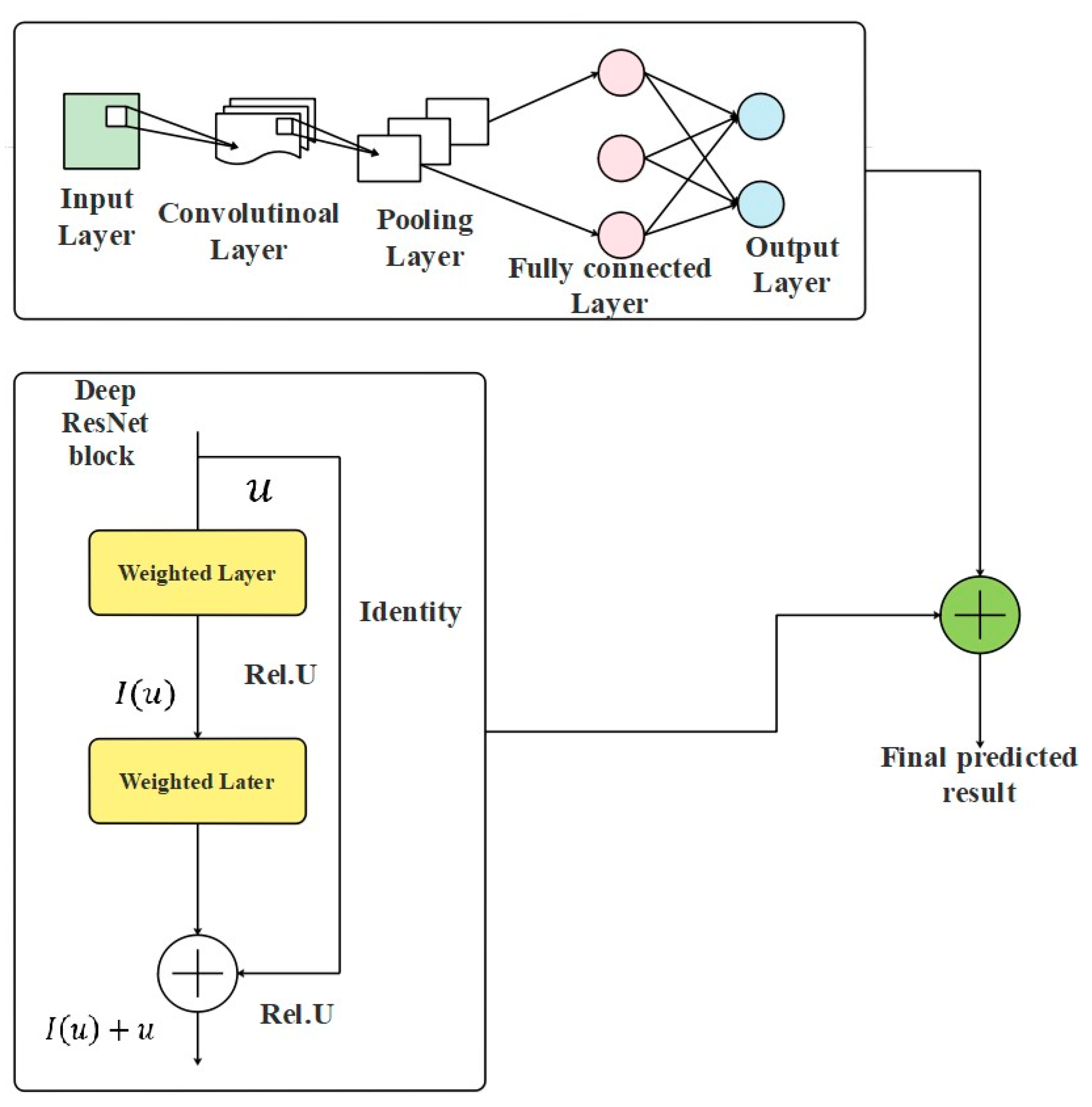
The final feature set F s e t is subjected to the hybrid model for flood prediction that trains with the extracted feature set. The hybrid model includes CNN and deep Residual Network (deep ResNet). The hybrid concept works in this way: the extracted feature set F s e t is subjected to both classifiers simultaneously, and the outcomes from them are averaged to obtain the final prediction results.

3.5.1. CNN Model

The input to CNN [35] is F s e t . A high-level review of CNNs in the area of classification is provided in this part, where convolutional, down sampling, and activation layers are some of the layers that make up CNNs; each layer applies a specific task to the incoming data. Initial convolutional layers inside the network retrieve low-level features, while subsequent layers extract more intricate semantic factors. These “extract features F s e t ” are then used for classification. The kernel weights S and CNN biases are learned from a set of input images through a technique known as back propagation. The main aspects of the images from any location are summarized by the kernel values, which are referred to as parameters. These kernel weights conduct an element-wise dot product as they travel across an input image, producing intermediate outcomes that are later added to the learned bias value. The result of each neuron is then defined by input; these results are referred to as activation maps. A different kind of layer, termed pooling, is used by CNNs to decrease the parameter count and assist in preventing overfitting. In a CNN, activation functions are employed to provide non-linearity, enabling the network to learn more intricate input patterns [36]. To conclude, CNNs develop spatially-aware depictions through many stacked layers of computation in contrast to traditional image classification models, which could be over-parameterized based on intrinsic characteristics in the image.

3.5.2. Deep ResNet Model

The input to deep ResNet [37] is F s e t . The fundamental advantage of ResNets is its capacity to build deep networks with a large number of weighted layers. Gradients from the loss function to the different layers find it increasingly challenging to back propagate without decreasing to zero or expanding as the depth of a network rises. By utilizing a skip link, ResNets enable gradients to travel over layers without being attenuated. The residual function I ( F s e t ) in Equation (11) is learned from the residual block D ( u ) , which is defined as follows:
D u = I F s e t + F s e t
By using labeled data to train the weight layers S , the residual function I ( F s e t ) is learned. Any form of neural network layer, such as fully connected or convolutional layers, may be used as weight layers. By declaring D u as 0 for particular sections of the network, the residual block enables the forward pass across the network to choose to skip over those sections. By using various feature extractor layers, each of which can extract a different potential characteristic of the input, it is now possible to construct an extremely deep network [38]. Only the sections of the network necessary for categorizing a given input case are activated for that instance [39]. Figure 2 represents the hybrid classification model combining CNN and deep ResNet.
Deep learning applications frequently experience the over-fitting issue, which has a detrimental effect on predicting fresh data. This specifically happens when the learning model is closely suited to the training data. In this study, a hybrid classification model named CNN and deep ResNet increases the amount of training data examples and the number of passes on the existing training data, which makes the model lightweight to overcome the over-fitting issue.

4. Training Phase: Combined Harris Hawks Shuffled Shepherd Optimization (CHHSSO) Algorithm

According to this study, the CNN and deep ResNet classifiers’ weight matrices S and S are fine-tuned using the CHHSSO approach, with an objective of error minimization. Weights S and S are provided as the input solution to the CHHSSO method. Equation (12) defines the given objective o b of CHHSSO, and e r denotes the error between predicted and actual value. As per this work, the flood is predicted, and the difference between the target value and the predicted value is estimated during the error calculation.
o b = M i n   e r
The CHHSSO algorithm is a combination of Harris hawks optimization (HHO) [40] and the shuffled shepherd optimization algorithm (SSOA) [41]. The solution update for HHO is performed by the SSOA according to the CHHSSO algorithm. The fundamental aim of HHO [42] was to reproduce the ordinary hunting behaviour of the hawk and prey’s motion to identify results for a single-objective problem.

4.1. Proposed Exploration Phase

This stage explains the hawks’ location while searching for its prey. It relies on two different methods. The first method describes how hawks locate prey based on the placements of the actual S i ,   i = 1 , 2 , , N , N represents the hawks’ count provided in Equation (13). The second method, however, describes how hawks identify prey based on their position on a random tree S r a n d which is depicted in Equation (14), where S i t + 1 indicates position update of hawks in succeeding iteration t , while S r a n d t indicates the hawks’ present position, r 1 , r 2 , r 3 , r 4 and q indicates the random integers within (0, 1). In Equation (15), S m t indicates the mean positions for overall hawks. However, as per the proposed logic, the S r a n d calculation is based on the best, worst, and current position, as specified in Equation (15). S p r e y t indicates the prey position.
S i t + 1 = S r a n d t r 1   S r a n d t 2 r 2 S t q 0.5 S p r e y t S m t U , q 0.5
Here, U = r 3 l b + r 4 u b l b
S t = i = 1 N S i t N
According to CHHSSO, S r a n d t is calculated in Equation (15).
S r a n d t = S b e s t t + S w o r s t t + S 3

4.2. Proposed Transition from Exploration to Exploitation

This phase of HHO tries to define and model how hawks modify their behaviour from the exploration stage to the exploitation stage. This behaviour is dependent on the prey’s escape energy E g , which is expressed in Equation (16).
E g = 2 E g 0 1 t t
According to CHHSSO, E g is calculated in Equation (17), where C is the chaotic random number estimated by the logistic map function. A polynomial map of degree 2 called the logistic map in Equation (18) is frequently used as a classic illustration of how extremely straightforward non-linear dynamical equations may produce complicated, chaotic behaviour.
E g = 2 C E g 0 1 t t
Φ k + 1 = a Φ k 1 Φ k
E g 0 refers to the prey’s initial energy; E g represents the escaping energy; t represents the iteration count; and t refers the maximum iteration.

4.3. Exploitation Phase

The primary two components of this stage are hawk hunting techniques and prey escape behaviours [43]. Around four strategies were followed in the exploitation stage:
  • soft besiege;
  • hard besiege;
  • soft besiege having progressive fast dives;
  • hard besiege having progressive fast dives.

4.3.1. Soft Besiege

Here, if E g 0.5 and r 0.5 , this method results in a single gentle besiege. The modelling of this behaviour is shown in Equation (19), where Δ S t in Equation (20) stands for the variations among the rabbit’s position vector and the new position in iteration t . The prey escape method, J p = 2 1 r 5 , varied at random throughout each iteration. r 5 indicates the random integer within (0, 1).
S i t + 1 = Δ S t E g J p   S p r e y t S t
Δ S t = S p r e y t S t

4.3.2. Hard Besiege

If E g 0.5 and r 0.5 , this method results in two hard besieges. The hawks’ position update is provided in Equation (21).
S i t + 1 = S p r e y t E g Δ S t
As per CHHSSO, the hawks’ position update is performed by the SSOA, which is provided in Equation (22).
S i n e w = S i b e s t + s t e p s i z e i + L e v y β

4.3.3. Soft Besiege: Having Progressive Fast Dives

Whenever the prey retains adequate power for effective escape, E g 0.5 and the hawks are still building a soft besiege r 0.5 , this method updates the hawks’ position. To increase the exploitation power as predicted by Equations (23) and (24), team fast dives depending on the levy flights that are carried out, where R indicates the problem dimension, L F in Equation (25) indicates the function of levy flight, and Q indicates the random vector with 1 × R size; V indicates the exploitation capacity.
U = S p r e y t E g J p   S p r e y t S t
V = U + Q × L F R
L F S = l × σ | m |   1 γ , σ = Γ 1 + γ × sin π γ 2 Γ 1 + γ 2 × γ × 2 γ 1 2 1 γ
where l , m indicates the random integer within (0, 1), and γ indicates the constant number assigned with 1.5. Furthermore, Equation (26) can be used to determine the hawks’ location update in soft besiege using the progressive fast dives approach.
S t + 1 = U   i f   Z U Z S t V   i f   Z V Z S t

4.3.4. Hard Besiege Having Progressive Fast Dives

Here, hawks built a hard besiege around r 0.5 ; prey is unable to escape E g 0.5 . This method is based on the hard besiege model given in Equation (27).
S t + 1 = U   i f   Z U Z S t V   i f   Z V Z S t
The pseudocode of CHHSSO is mentioned in Algorithm 1.
Algorithm 1: Pseudocode of CHHSSO
Input: S and S
Output: S ¯ and S ¯ (Optimal weights)
Initialize: S i ,   i = 1 , 2 , , N
While end step is not reached do
Compute hawks’ fitness value
Assign S p r e y as prey position (best position)
for each hawk S i do
Update jump strength J p as well as initial energy E g o
J p = 2 1 r a n d , E g o = 2   r a n d 1
Update E g as per the proposed Equation (17) with logistic map randomization
Update vector position using Equation (13), with new S r a n d t calculation
if E g 1 then
if E g 0.5 and r 0.5
Update vector position by Equation (19)
     end if
end if
else if E g 0.5 and r 0.5 then
Update vector position by Equation (22) as per CHHSSO
else if E g 0.5 and r 0.5
Update vector position by Equation (26)
else if E g 0.5 and r 0.5 then
Update vector position by Equation (27)
               end if
          end if
     end if
end for
end while
Return S p r e y

5. Results and Discussion

The proposed flood detection in the satellite image is implemented in PYTHON. The operating system requires Windows 11, Mac OS X 10.11, 64-bit Linux, CPU (Intel), RHEL 6/7, 16 GB of RAM, and 5 GB of free disk space. The following experimental setups are used:
  • type of network: CNN and deep ResNet models.
  • learning percentage: 60, 70, 80, and 90.
  • Bands: coastal aerosol, blue, green, red, vegetation red edge, vegetation red edge, vegetation red edge, NIR, vegetation red edge, water vapour, SWIR-curris, SWIR, and SWIR.
  • Batch parameter: 32.
  • Epochs parameter: 50.
To assess the results of the different networks, performances such as accuracy, precision, sensitivity, specificity, FPR, FNR, NPV, F-measure, and MCC are formulated using Equations (28)–(36), respectively.
A c c u r a c y = T P + T N T P + T N + F P + F N
P r e c i s i o n = T P T P + F P = 1 F D R
S e n s i t i v i t y = T P T P + F N = 1 F N R
S p e c i f i c i t y = T N T N + F P = 1 F P R
F P R = F P F P + T N = 1 T N R
F N R = F N F N + T P = 1 T P R
N P V = T N T N + F N = 1 F O R
F m e a s u r e = 2 T P 2 T P + F P + F N
M C C = T P × T N F P × F N T P + F P + T P + F N + T N + F P + ( T P + F N )
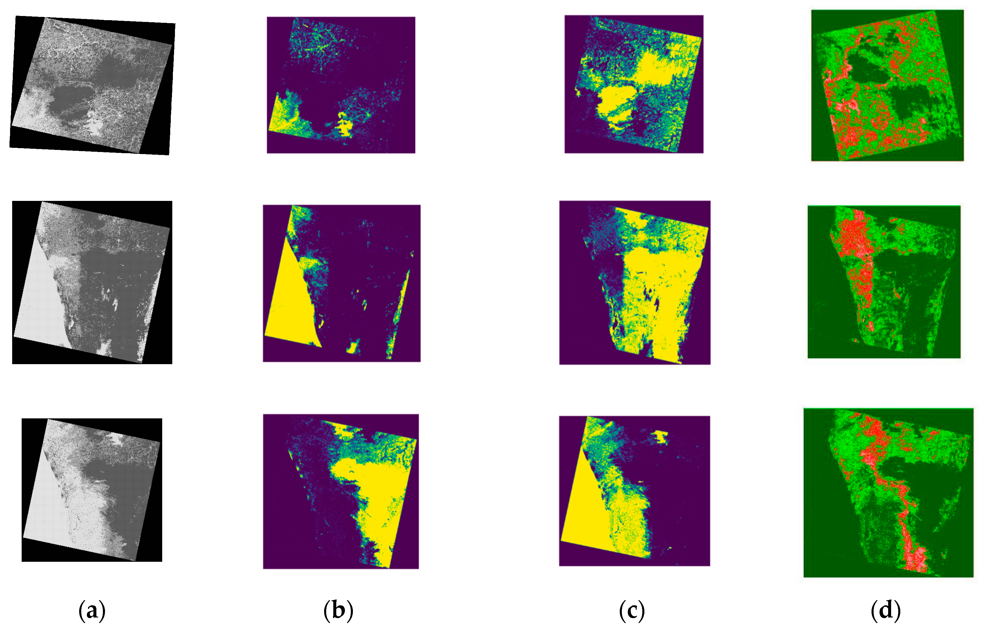
The assessment of the deep hybrid model for flood prediction with CHHSSO-based training (DHMFP) is performed over deep belief networks (DBN), recurrent neural networks (RNN), long short term memory (LSTM), support vector machines (SVM), bidirectional gated recurrent units (Bi-GRU), shuffled shepherd optimization algorithm (SSOA), Harris hawks optimization (HHO), COOT, arithmetic optimization algorithm (AOA), change detection (CD) approach [12], and fully convolutional neural networks (FCNN) [19], regarding accuracy, NPV, FPR, and so on. To further illustrate the effectiveness of the DHMFP, statistical analysis, an ablation study, and segmentation accuracy are performed and tested. Additionally, the original and segmented images are displayed in Figure 3.
In Figure 3, the first column (a) represents the sample images that were taken from the collected dataset. While the second column (b) represents the segmented image using the conventional k-means algorithm, where it overlaps with the pre-existing data, it therefore fails to find a better portion for flood-affected regions. The third column (c) represents the segmented image using the FCM method, which is one of the most common methods of image segmentation. However, this method does not have the capability to distinguish objects with similar colour intensity. Initially, it detected the flooded region; after some time, it detected the static regions near flood areas; therefore, the accuracy of this method is nearly low. Finally, the fourth column (d) represents the segmented image performed by the proposed DHMFP method. Here, the flood regions (paths) are detected accurately without overlapping with the pre-existing data. From that image, the greenish portion denotes the overall affected area, while the orange-coloured portions denote the path of flooding flowing through the affected regions.

5.1. Analysis of DHMFP with Regard to Positive Measures

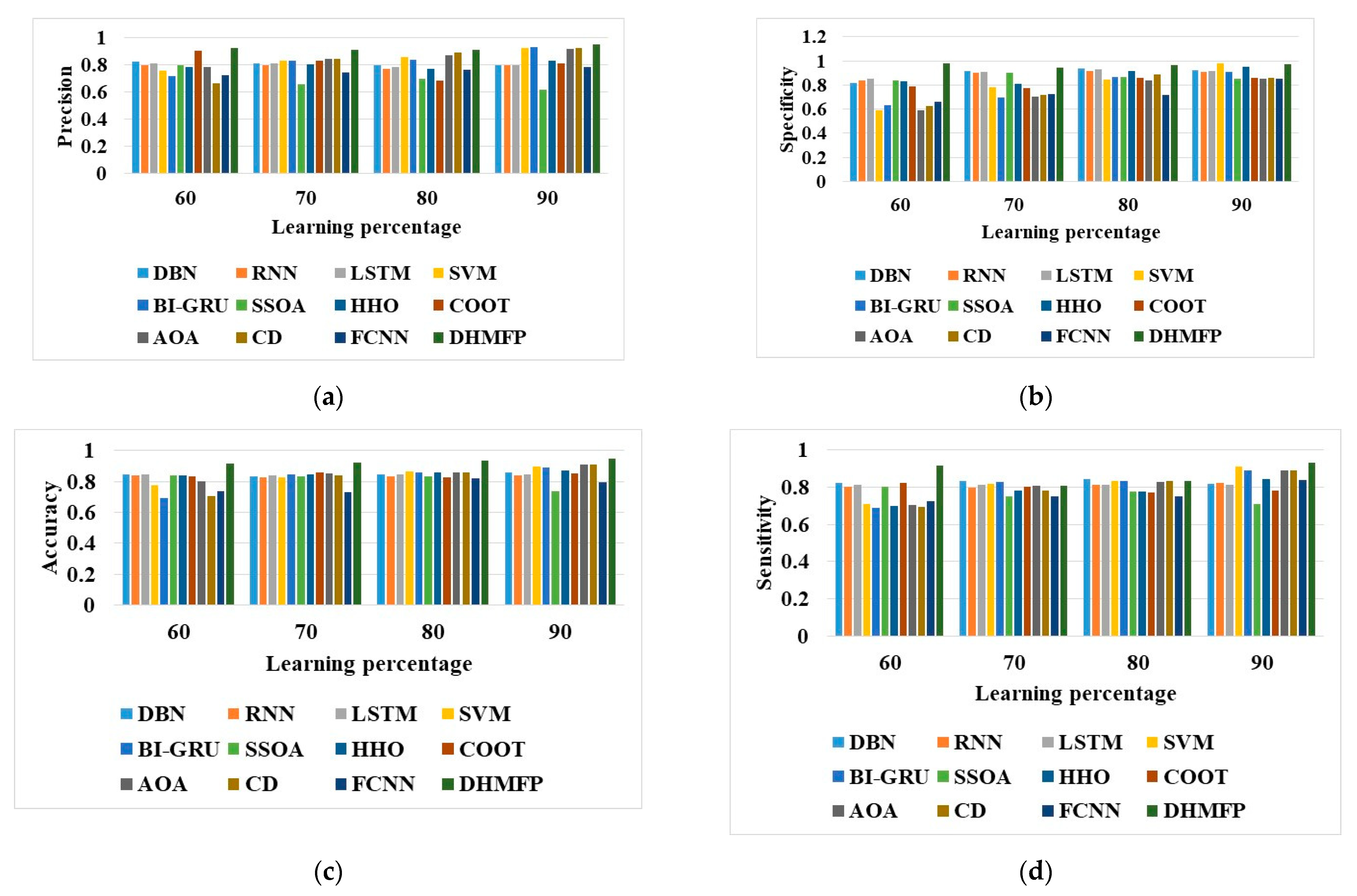
The review of DHMFP for flood detection in satellite images is evaluated against DBN, RNN, LSTM, SVM, Bi-GRU, SSOA, HHO, COOT, AOA, CD, and FCNN for numerous measures, as exhibited in Figure 4. In Figure 4a, a higher precision of approximately 90.92% is accomplished by DHMFP at the learning percentage of 80; though, DBN is 0.796, RNN is 0.771, LSTM is 0.784, SVM is 0.859, Bi-GRU is 0.835, SSOA is 0.695, HHO is 0.769, COOT is 0.681, AOA is 0.872, CD is 0.889, and FCNN is 0.76, respectively. When the learning percentage is adjusted to 60, DHMFP reaches a specificity of 98.29%, whilst the specificity of other classifiers is as follows: DBN = 81.34%, RNN = 84.43%, LSTM = 85.56%, SVM = 58.74%, Bi-GRU = 63.57%, SSOA = 83.91%, HHO = 82.80%, COOT = 78.55%, AOA = 59.18%, CD = 62.78%, and FCNN = 65.86%.
For 90% of the learning percentage, the DHMFP generated an accuracy of 94.98%; at the same time, the DBN, RNN, LSTM, SVM, BI-GRU, SSOA, HHO, COOT, AOA, CD, and FCNN generated a lesser accuracy of 85.67%, 83.91%, 84.74%, 89.68%, 88.19%, 73.85%, 86.93%, 84.98%, 90.58%, 91.17%, and 79.54%, respectively. The sensitivity obtained by the DHMFP at the 90th learning percentage is 93.48%, whereas at the 70th learning percentage, the sensitivity recorded by the DHMFP is 80.97%. Simultaneously, the sensitivity maintained by DHMFP at the 80th learning percentage is 83.65%, even though at the 60th learning percentage, the sensitivity established by DHMFP is 91.89%. Thereby, it affirms the possibility of the DHMFP’s the flood detection in satellite images.

5.2. Analysis of DHMFP with Regard to Negative Measures

The study on DHMFP based on flood detection in satellite images is estimated over DBN, RNN, LSTM, SVM, Bi-GRU, SSOA, HHO, CCOT, AOA, CD, and FCNN, as described in Figure 5a,b. At the 90th learning percentage, the DHMFP offered the FNR of 0.02, which is contrasted to DBN = 0.152, RNN = 0.185, LSTM = 0.174, SVM = 0.005, Bi-GRU = 0.009, SSOA = 0.283, HHO = 0.125, COOT = 0.208, AOA = 0.086, CD = 0.088, and FCNN = 0.091, respectively. DHMFP yielded the lowest FPR of 0.024, whilst the DBN, RNN, LSTM, SVM, Bi-GRU, SSOA, HHO, COOT, AOA, CD, and FCNN obtained the FPR of 0.083, 0.094, 0.089, 0.236, 0.338, 0.098, 0.094, 0.134, 0.036, 0.188, 0.34, and 0.273, respectively. Thus, the DHMFP’s supremacy over other traditional classifiers in terms of negative metrics is revealed.

5.3. Analysis of DHMFP with Regard to Other Measures

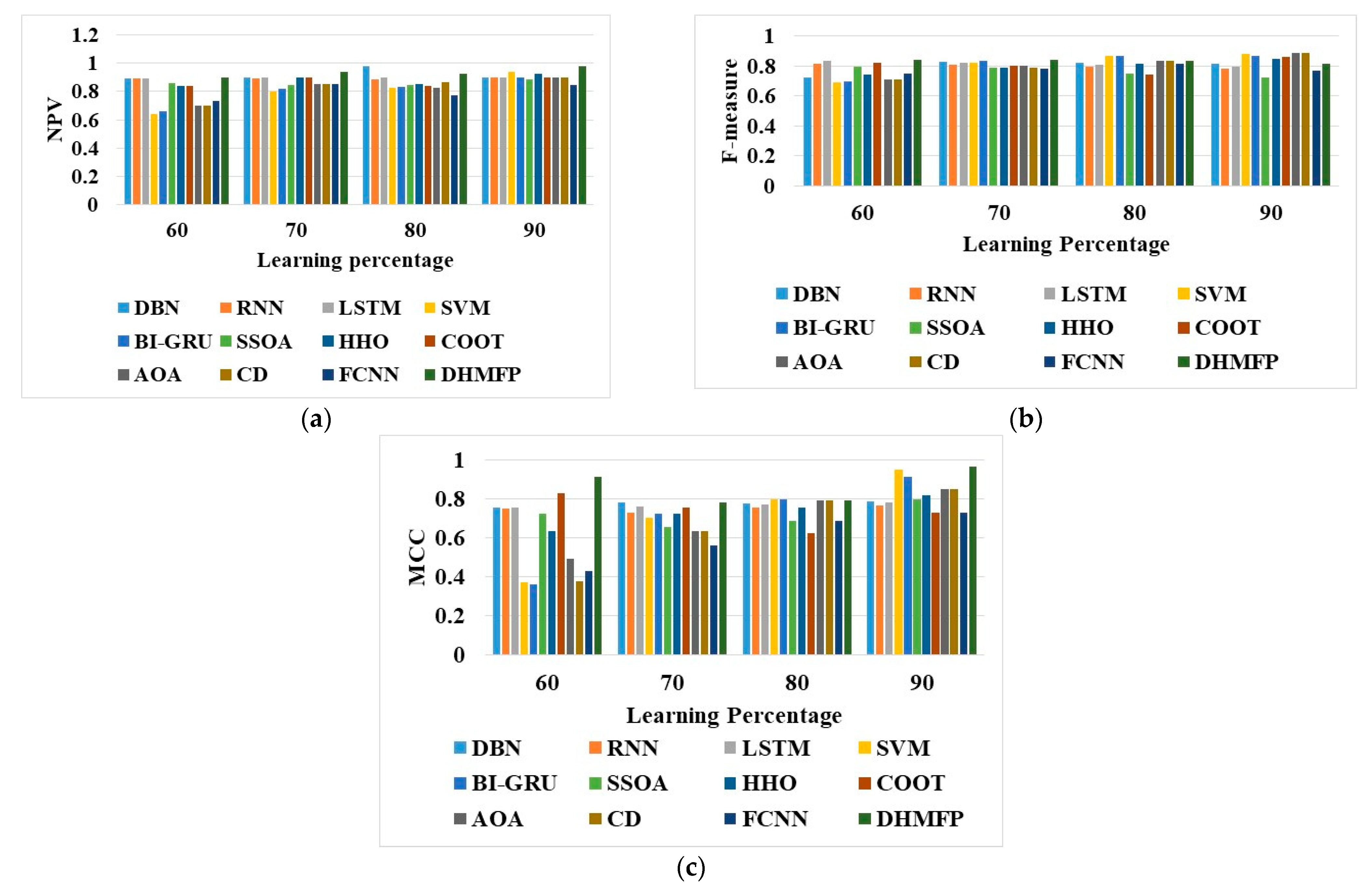
DHMFP is contrary to numerous previous models in terms of NPV, F-measure, and MCC, as shown in Figure 6a–c. In particular, the NPV of DHMFP for the 80th learning percentage is 0.927, whereas the conventional methods scored a very low NPV. Notably, DBN is 0.908, RNN is 0.885, LSTM is 0.899, SVM is 0.826, Bi-GRU is 0.835, SSOA is 0.849, HHO is 0.855, COOT is 0.842, AOA is 0.829, CD is 0.869, and FCNN is 0.772, respectively. When the learning percentage is set to 90%, the classifiers DBN, RNN, LSTM, SVM, Bi-GRU, SSOA, HHO, COOT, AOA, CD, and FCNN obtained the f-measures of 81.83%, 78.29%, 79.87%, 87.93%, 86.64%, 72.56%, 84.62%, 85.83%, 88.74%, 88.98%, and 77.24%, respectively. Simultaneously, the DHMFP MCC at the 60th learning percentage is 91.28%, while at the 90th learning percentage it produces an MCC of 96.37%. Therefore, the DHMFP provides enhanced flood detection performance due to the considerable enhancement of the other measures.

5.4. Ablation Study DHMFP

The ablation study of the model without optimization, the model with conventional k-means, and DHMFP is delineated in Table 2. Flood prediction without CHHSSO, flood prediction with cubic chaotic map weighted based k-means clustering, and DHMFP acquired precisions of 89.22%, 87.65%, and 93.65%, respectively. The FPR of the flood prediction without CHHSSO = 0.105, flood prediction with cubic chaotic map weighted based k-means clustering = 0.136, and DHMFP = 0.036. The accuracy, FNR, and NPV of the DHMFP are 95.21%, 0.085797, and 90.59%, respectively.

5.5. Prediction Error Statistics on the Performance of DHMFP over Traditional Systems

A statistical analysis of five case scenario studies, including the standard deviation, mean, best, median, and worst, is performed in order to examine the efficacy of DHMFP flood detection in satellite images. Additionally, the DHMFP is appraised over DBN, RNN, LSTM, SVM, Bi-GRU, SSOA, HHO, COOT, AOA, CD, and FCNN, and the outcomes are provided in Table 3. While giving consideration to the best-case scenario, the DHMFP maintained an error rate of 0.034, though the DBN has 0.113, RNN has 0.132, LSTM has 0.119, SVM has 0.124, Bi-GRU has 0.144, SSOA has 0.170, HHO has 0.131, COOT has 0.153, AOA has 0.123, CD has 0.163, and FCNN has 0.226, respectively. Thus, it has been ascertained that the DHMFP is adequate for flood detection in satellite images.

5.6. Assessment of Segmentation Performance

The analysis of the segmentation performance of the DHMFP is contrasted to conventional k-means, FCM, and OmbriaNet–CNN [22], which are represented in Table 4. The dice score of the improved k-means is 0.863, whilst the conventional k-means is 0.676 and the FCM is 0.787. The Jaccard coefficient of the improved k-means is 0.889, while the conventional k-means and FCM gained the Jaccard coefficients of 0.732 and 0.739. Additionally, analysing the segmentation accuracy, the improved k-means are proven to have a higher rating of 0.894 than the conventional k-means, FCM and OmbriaNet–CNN [22], which have obtained lower values of 0.785, 0.654, and 0.865, respectively.

5.7. Convergence Analysis

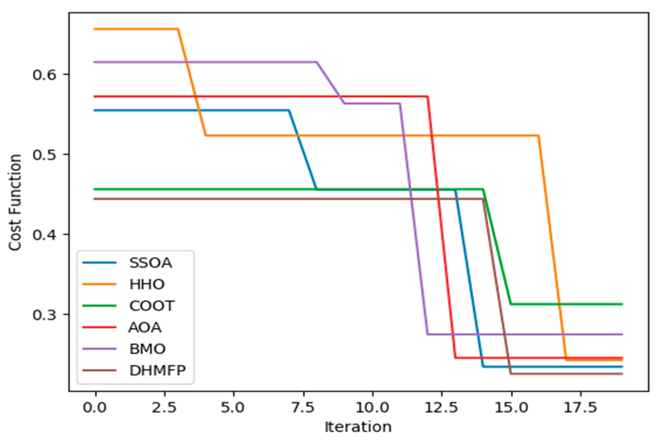
In order to indicate the pre-eminences of the DHMFP in flood detection, it is evaluated over the DBN, RNN, LSTM, SVM, Bi-GRU, SSOA, HHO, COOT, AOA, CD, and FCNN, which are exposed in Figure 7. The DHMFP attains an error rate of approximately 0.45 during the first iteration; this is less than SSOA (0.54), HHO (0.75), COOT (0.48), AOA (0.59), and BMO (0.63). During the 17.5th iteration, the DHMFP had an error value of 0.63; meanwhile, the SSOA, HHO, COOT, AOA, and BMO maintained error values of 0.21, 0.23, 0.34, 0.22, and 0.29, respectively. This highlights that DHMFP can afford precise outcomes for flood detection in satellite images.

5.8. Analysis of Training and Validation Losses

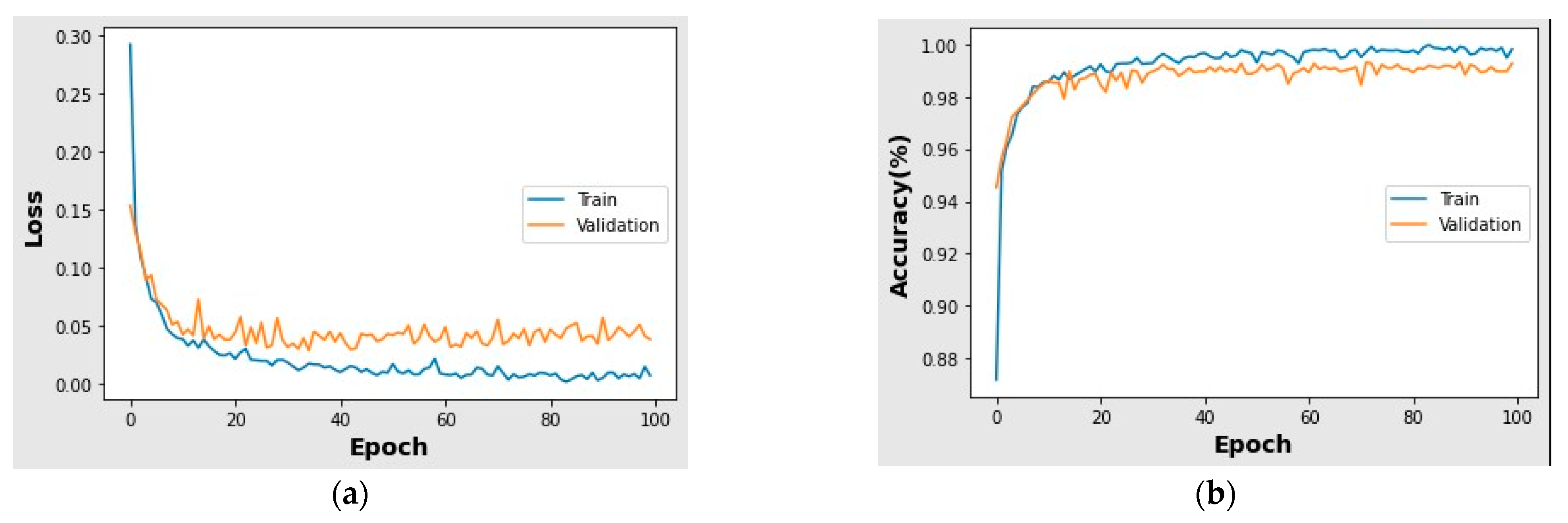
One of the most widely used metrics is the ratio of training loss to validation loss over time. While the training loss indicates how effectively the model matches training data, the validation loss indicates how well the model matches new data. The graphical depiction of training and validation loss is exposed in Figure 8a, which shows that the training loss started to decrease and reached a value of 0.02 over 100 epochs, while the validation loss reached a value of 0.05 over the same time period. While training accuracy denotes the accuracy of trained data, validation accuracy denotes the accuracy of new data. Figure 8b shows the graphical representation of training and validation accuracy. From Figure 8b, it clearly displays that training accuracy starts at 0.9894 at 100 epochs, while validation accuracy achieves 0.9813 at 100 epochs.

5.9. Discussion

Here, a novel deep hybrid model for flood prediction (DHMFP) based CHHSSO is suggested for flood prediction. The proposed CHHSSO based on DHMFP is compared to a number of existing models, including OmbriaNet-CNN [22], DBN, RNN, LSTM, SVM, Bi-GRU, SSOA, HHO, COOT, AOA, CD, and FCNN. The improved k-means have attained a dice score (0.863), Jaccard coefficient (0.889), and segmented accuracy (0.894) for the segmentation study. The final extracted feature set is used to perform hybrid classification using CNN and deep ResNet classifiers to obtain the final feature set. The CHHSSO algorithm then adjusts the weight of CNN and deep ResNet. For that analysis, the proposed DHMFP receives the following values from the results: sensitivity = 93.48%, specificity = 98.29%, accuracy = 94.98%, FNR = 0.02%, and FPR = 0.02%. The effectiveness of DHMFP flood detection in satellite images is investigated using a statistical analysis, which is elaborated in Table 2. These analyses clearly demonstrate that the suggested DHMFP maintains an error rate of 0.034 despite the values of DBN (0.113), RNN (0.132), LSTM (0.119), SVM (0.124), Bi-GRU (0.144), SSOA (0.170), HHO (0.131), COOT (0.153), AOA (0.123), CD (0.163), and FCNN (0.226). Furthermore, the proposed DHMFP–CHHSSO displays better performances in terms of sensitivity (0.932), specificity (0.977), accuracy (0.952), false negative rate (0.0858), and false positive fate (0.036), respectively. While considering the segmentation performance, improved k-means are compared with conventional k-means, FCM, and OmbriaNet–CNN [22]. From the analysis, it clearly shows that an improved k-means achieved a higher accuracy of 0.894, while other methods have 0.785, 0.654, and 0.865, respectively. Hence, from the overall analysis, it is determined that the proposed DHMFP is sufficient for flood detection in satellite images when compared with other existing models.

6. Conclusions

This research developed a new deep hybrid model for flood prediction with the CHHSSO-based training (DHMFP) algorithm. Here, the input satellite image was preprocessed using the MF approach. The preprocessed image was then segmented using the improved k-means clustering procedure. After that, depending on the segmented image, features like DVI, NDVI, MTVI, GVI, and SAVI were extracted. Using the final extracted feature set, hybrid classification was performed. The final feature set was given as an input to both the CNN and deep ResNet classifiers. The output obtained from both optimized classifiers was averaged to obtain the final predicted outcome. The fine tuning of CNN and deep ResNet weight was performed by the combined Harris hawks shuffled shepherd optimization (CHHSSO) algorithm. Furthermore, the CHHSSO’s performance was assessed, and the results were effectively validated. According to the findings, the proposed DHMFP obtained the following values for sensitivity, specificity, accuracy, and FNR: 93.48%, 98.29%, 94.98%, and 0.02 and 0.02, correspondingly. To evaluate the effectiveness of the DHMFP flood detection in satellite images, a statistical study was performed that included the standard deviation, mean, best, median, and worst. Based on that data, it was evident that the proposed DHMFP maintained an error rate of 0.034 even though the DBN, RNN, LSTM, SVM, Bi-GRU, SSOA, HHO, COOT, AOA, 0.123, CD, and FCNN all had values of 0.113, 0.132, 0.119, 0.124, 0.144, 0.144, 0.144, 0.131, 0.131, 0.153, 0.153, 0.123, and 0.163, respectively.
The ability of CNNs to learn directly from raw pixel data without the necessity for manual feature engineering or preprocessing is one of their key advantages. This means that the most prominent aspects of the images, such as edges, forms, colours, textures, and objects, may be automatically discovered and adapted to. This also makes the training and inference processes faster and more effective by reducing the dimensionality and complexity of the input data. However, ResNet, a potent deep neural network architecture, has transformed the area of computer vision by making it possible to build deeper and more precise networks. ResNet is complicated, prone to overfitting, and has poor interpretability, among other drawbacks. To overcome the above-stated limitations and improve the classification accuracy of flood prediction models, this research can be further extended by analysing unique deep learning with additional hybrid combinations of optimization techniques.

Author Contributions

The paper investigation, resources, data curation, writing—original draft preparation, writing—review and editing, and visualization were conducted by H.D.P. and R.H.K. The paper conceptualization and software were conducted by K.R.C. and B.B.B. The validation and formal analysis, methodology, supervision, project administration, and funding acquisition of the version to be published were conducted by A.S. All authors have read and agreed to the published version of the manuscript.

Funding

This research received no external funding.

Data Availability Statement

Not applicable.

Conflicts of Interest

The authors declare no conflict of interest.

References

  1. Luis, C.; Alvarez, M.; Puertas, J. Estimation of flood-exposed population in data-scarce regions combining satellite imagery and high resolution hydrological-hydraulic modelling: A case study in the Licungo basin (Mozambique). J. Hydrol. Reg. Stud. 2022, 44, 101247. [Google Scholar]
  2. Mohammed Sarfaraz, G.A.; Siam, Z.S.; Kabir, I.; Kabir, Z.; Ahmed, M.R.; Hassan, Q.K.; Rahman, R.M.; Dewan, A. A novel framework for addressing uncertainties in machine learning-based geospatial approaches for flood prediction. J. Environ. Manag. 2023, 326, 116813. [Google Scholar]
  3. Roberto, B.; Isufi, E.; NicolaasJonkman, S.; Taormina, R. Deep Learning Methods for Flood Mapping: A Review of Existing Applications and Future Research Directions. Hydrol. Earth Syst. Sci. 2022, 26, 4345–4378. [Google Scholar]
  4. Kim, H.I.; Han, K.Y. Data-Driven Approach for the Rapid Simulation of Urban Flood Prediction. KSCE J. Civ. Eng. 2020, 24, 1932–1943. [Google Scholar] [CrossRef]
  5. Kim, H.I.; Kim, B.H. Flood Hazard Rating Prediction for Urban Areas Using Random Forest and LSTM. KSCE J. Civ. Eng. 2020, 24, 3884–3896. [Google Scholar] [CrossRef]
  6. Keum, H.J.; Han, K.Y.; Kim, H.I. Real-Time Flood Disaster Prediction System by Applying Machine Learning Technique. KSCE J. Civ. Eng. 2020, 24, 2835–2848. [Google Scholar] [CrossRef]
  7. Thiagarajan, K.; Manapakkam Anandan, M.; Stateczny, A.; Bidare Divakarachari, P.; Kivudujogappa Lingappa, H. Satellite image classification using a hierarchical ensemble learning and correlation coefficient-based gravitational search algorithm. Remote Sens. 2021, 13, 4351. [Google Scholar] [CrossRef]
  8. Jagannathan, P.; Rajkumar, S.; Frnda, J.; Divakarachari, P.B.; Subramani, P. Moving vehicle detection and classifi-cation using gaussian mixture model and ensemble deep learning technique. Wirel. Commun. Mob. Comput. 2021, 2021, 5590894. [Google Scholar] [CrossRef]
  9. Simeon, A.I.; Edim, E.A.; Eteng, I.E. Design of a flood magnitude prediction model using algorithmic and mathematical approaches. Int. J. Inf. Tecnol. 2021, 13, 1569–1579. [Google Scholar] [CrossRef]
  10. Aarthi, C.; Ramya, V.J.; Falkowski-Gilski, P.; Divakarachari, P.B. Balanced Spider Monkey Optimization with Bi-LSTM for Sustainable Air Quality Prediction. Sustainability 2023, 15, 1637. [Google Scholar] [CrossRef]
  11. Huynh, H.X.; Loi, T.T.T.; Huynh, T.P.; Van Tran, S.; Nguyen, T.N.T.; Niculescu, S. Predicting of Flooding in the Mekong Delta Using Satellite Images. In Context-Aware Systems and Applications, and Nature of Computation and Communication; Vinh, P., Rakib, A., Eds.; Lecture Notes of the Institute for Computer Sciences, Social Informatics and Telecommunications Engineering; Springer: Cham, Switzerland, 2019; p. 298. [Google Scholar] [CrossRef]
  12. Mitchell, D.G.; Li, S.; Lindsey, D.T.; Sjoberg, W.; Zhou, L.; Sun, D. Mapping, Monitoring, and Prediction of Floods Due to Ice Jam and Snowmelt with Operational Weather Satellites. Remote Sens. 2020, 12, 1865. [Google Scholar] [CrossRef]
  13. Anastasia, M.; Bakratsas, M.; Andreadis, S.; Karakostas, A.; Gialampoukidis, I.; Vrochidis, S.; Kompatsiaris, I. Flood detection with Sentinel-2 satellite images in crisis management systems. In Proceedings of the 17th ISCRAM Conference, Blacksburg, VA, USA, 24–27 May 2020. [Google Scholar]
  14. Du, J. Satellite Flood Inundation Assessment and Forecast Using SMAP and Landsat. IEEE J. Sel. Top. Appl. Earth Obs. Remote Sens. 2021, 14, 6707–6715. [Google Scholar] [CrossRef] [PubMed]
  15. Mateo-Garcia, G.; Veitch-Michaelis, J.; Smith, L.; Oprea, S.V.; Schumann, G.; Gal, Y.; Baydin, A.G.; Backes, D. Towards global flood mapping onboard low-cost satellites with machine learning. Sci. Rep. 2021, 11, 1–12. [Google Scholar] [CrossRef]
  16. Sayak, P.; Ganju, S. Flood Segmentation on Sentinel-1 SAR Imagery with Semi-Supervised Learning. arXiv 2021, arXiv:2107.08369. [Google Scholar]
  17. Löwe, R.; Böhm, J.; Jensen, D.G.; Leandro, J.; Rasmussen, S.H. U-FLOOD—Topographic deep learning for predicting urban pluvial flood water depth. J. Hydrol. 2021, 603, 126898. [Google Scholar] [CrossRef]
  18. Motta, M.; de Castro Neto, M.; Sarmento, P. A mixed approach for urban flood prediction using Machine Learning and GIS. Int. J. Disaster Risk Reduct. 2021, 56, 102154. [Google Scholar] [CrossRef]
  19. Panahi, M.; Jaafari, A.; Shirzadi, A.; Shahabi, H.; Rahmati, O.; Omidvar, E.; Lee, S.; Bui, D.T. Deep learning neural networks for spatially explicit prediction of flash flood probability. Geosci. Front. 2021, 12, 101076. [Google Scholar] [CrossRef]
  20. Dazzi, S.; Vacondio, R.; Mignosa, P. Flood stage forecasting using machine-learning methods: A case study on the Parma River (Italy). Water 2021, 13, 1612. [Google Scholar] [CrossRef]
  21. Lei, X.; Chen, W.; Panahi, M.; Falah, F.; Rahmati, O.; Uuemaa, E.; Kalantari, Z.; Ferreira, C.S.; Rezaie, F.; Tiefenbacher, J.P.; et al. Urban flood modeling using deep-learning approaches in Seoul, South Korea. J. Hydrol. 2021, 601, 126684. [Google Scholar] [CrossRef]
  22. Drakonakis, G.I.; Tsagkatakis, G.; Fotiadou, K.; Tsakalides, P. OmbriaNet—Supervised flood mapping via convolutional neural networks using multitemporal sentinel-1 and sentinel-2 data fusion. IEEE J. Sel. Top. Appl. Earth Obs. Remote Sens. 2022, 15, 2341–2356. [Google Scholar] [CrossRef]
  23. Anzhelika, T.K.; Kuznetsova, I.A.; Levin, E.L. Prediction of the flooding area of the northeastern Caspian Sea from satellite images. Geod. Geodyn. 2022, 14, 191–200. [Google Scholar]
  24. Ahad Hasan, T.; McRae, C.B.; Tavakol-Davani, H.; Goharian, E. Flood Detection in Urban Areas Using Satellite Imagery and Machine Learning. Water 2022, 14, 1140. [Google Scholar] [CrossRef]
  25. Li, P.; Zhang, J.; Krebs, P. Prediction of flow based on a CNN-LSTM combined deep learning approach. Water 2022, 14, 993. [Google Scholar] [CrossRef]
  26. Before and after the Kerala Floods. Available online: https://earthobservatory.nasa.gov/images/92669/before-and-after-the-kerala-floods (accessed on 2 February 2023).
  27. Yuqin, S.; Liu, J. An improved adaptive weighted median filter algorithm. IOP Conf. Ser. J. Phys. Conf. Ser. 2019, 1187, 042107. [Google Scholar] [CrossRef]
  28. Saptarshi, C.; Paul, D.; Das, S.; Xu, J. Entropy Weighted Power k-Means Clustering. In Proceedings of the 23rd International Conference on Artificial Intelligence and Statistics (AISTATS) 2020, Palermo, Italy, 26–28 August 2020; p. 108. [Google Scholar]
  29. Moghimi, A.; Khazai, S.; Mohammadzadeh, A. An improved fast level set method initialized with a combination of k-means clustering and Otsu thresholding for unsupervised change detection from SAR images. Arab. J. Geosci. 2017, 10, 1–8. [Google Scholar] [CrossRef]
  30. Ghosh, A.; Mishra, N.S.; Ghosh, S. Fuzzy clustering algorithms for unsupervised change detection in remote sensing images. Inf. Sci. 2011, 181, 699–715. [Google Scholar] [CrossRef]
  31. Hui, L.; Wang, X.; Fei, Z.; Qiu, M. The Effects of Using Chaotic Map on Improving the Performance of Multiobjective Evolutionary Algorithms. Hindawi Publ. Corp. Math. Probl. Eng. 2014, 2014, 924652. [Google Scholar] [CrossRef]
  32. Broadband Greenness. Available online: https://www.l3harrisgeospatial.com/docs/broadbandgreenness.html (accessed on 2 February 2023).
  33. Driss, H.; Millera, J.R.; Pattey, E.; Zarco-Tejadad, P.J.; Ian, B.S. Hyperspectral Vegetation Indices and Novel Algorithms for Predicting Green LAI of Crop Canopies: Modeling and Validation in the Context of Precision Agriculture; Elsevier Inc.: Amsterdam, The Netherlands, 2004. [Google Scholar] [CrossRef]
  34. Martinez, J.C.; De Swaef, T.; Borra-Serrano, I.; Lootens, P.; Barrero, O.; Fernandez-Gallego, J.A. Comparative leaf area index estimation using multispectral and RGB images from a UAV platform. In Proceedings of the Autonomous Air and Ground Sensing Systems for Agricultural Optimization and Phenotyping VIII, Orlando, FL, USA, 13 June 2023; SPIE: Bellingham, WA, USA, 2023; Volume 12539, pp. 56–67. [Google Scholar]
  35. Zijie, J.W.; Turko, R.; Shaikh, O.; Park, H.; Das, N.; Hohman, F.; Kahng, M.; Horng, D. CNN EXPLAINER: Learning Convolutional Neural Networks with Interactive Visualization. arXiv 2020, arXiv:2004.15004v3. [Google Scholar]
  36. Ramayanti, S.; Nur, A.S.; Syifa, M.; Panahi, M.; Achmad, A.R.; Park, S.; Lee, C.W. Performance comparison of two deep learning models for flood susceptibility map in Beira area, Mozambique. Egypt. J. Remote Sens. Space Sci. 2022, 25, 1025–1036. [Google Scholar] [CrossRef]
  37. Aiden, N.; He, Z.; Wollersheim, D. Pulmonary nodule classification with deep residual networks. Int. J. Comput. Assist. Radiol. Surg. 2017, 10, 1799–1808. [Google Scholar] [CrossRef]
  38. Liu, J.; Liu, K.; Wang, M. A Residual Neural Network Integrated with a Hydrological Model for Global Flood Susceptibility Mapping Based on Remote Sensing Datasets. Remote Sens. 2023, 15, 2447. [Google Scholar] [CrossRef]
  39. Jackson, J.; Yussif, S.B.; Patamia, R.A.; Sarpong, K.; Qin, Z. Flood or Non-Flooded: A Comparative Study of State-of-the-Art Models for Flood Image Classification Using the FloodNet Dataset with Uncertainty Offset Analysis. Water 2023, 15, 875. [Google Scholar] [CrossRef]
  40. Hamzeh, M.A.; Alarabiat, D.; Abualigah, L.; Asghar Heidari, A. Harris hawks’ optimization: A comprehensive review of recent variants and applications. Neural Comput. Appl. 2021, 33, 8939–8980. [Google Scholar] [CrossRef]
  41. Ali, K.; Zaerreza, A.; Milad Hosseini, S. Shuffled Shepherd Optimization Method Simplified for Reducing the Parameter Dependency. Iran. J. Sci. Technol. Trans. Civ. Eng. 2021, 15, 1397–1411. [Google Scholar] [CrossRef]
  42. Parsa, P.; Naderpour, H. Shear strength estimation of reinforced concrete walls using support vector regression improved by Teaching–learning-based optimization, Particle Swarm optimization, and Harris Hawks Optimization algorithms. J. Build. Eng. 2021, 44, 102593. [Google Scholar] [CrossRef]
  43. Murlidhar, B.R.; Nguyen, H.; Rostami, J.; Bui, X.; Armaghani, D.J.; Ragam, P.; Mohamad, E.T. Prediction of flyrock distance induced by mine blasting using a novel Harris Hawks optimization-based multi-layer perceptron neural network. J. Rock Mech. Geotech. Eng. 2021, 13, 1413–1427. [Google Scholar] [CrossRef]
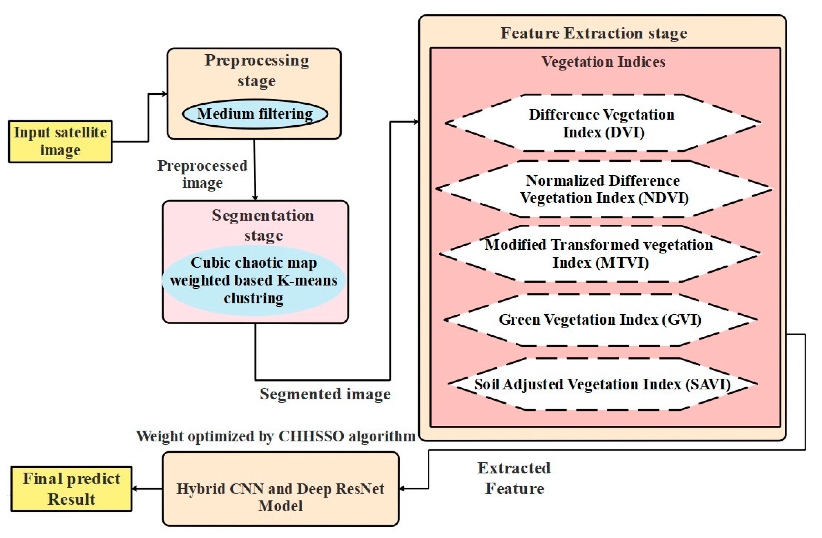
Figure 1. Pictorial representation of the DHMFP model.
Remotesensing 15 05037 g001
Figure 2. Hybrid classification model combining CNN and deep ResNet.
Remotesensing 15 05037 g002
Figure 3. Original and segmented images for flood detection in satellite images. (a) Sample images; (b) images segmented using conventional k-means; (c) using the FCM method; and (d) using the proposed DHMFP.
Remotesensing 15 05037 g003
Figure 4. Positive measure analysis (DHMFP versus conventional schemes): (a) precision; (b) specificity; (c) accuracy; and (d) sensitivity.
Remotesensing 15 05037 g004
Figure 5. Negative measure analysis (DHMFP versus conventional schemes): (a) FNR; (b) FPR.
Remotesensing 15 05037 g005
Figure 6. Other measure analysis (DHMFP versus conventional schemes): (a) NPV; (b) F-measure; (c) MCC.
Remotesensing 15 05037 g006
Figure 7. Convergence assessment on DHMFP vs. existing methods.
Remotesensing 15 05037 g007
Figure 8. (a) Depiction of training and validation losses, and (b) representation of training and validation accuracy.
Remotesensing 15 05037 g008
Table 1. Spectral indices for feature extraction.
IndexDefinitionEquation
DVI [32]This index can differentiate between vegetation and soil, but it cannot distinguish between radiance and reflectance that result from atmospheric factors or shadows. DVI is calculated in Equation (5). D V I = S b = 2 I S b = 1 I (5)
NDVI [32]NDVI is robust in a variety of situations due to the normalized difference formulations it uses, together with the maximum reflectance and absorption areas of chlorophyll. The NDVI is a metric of rich, healthy vegetation that is calculated using Equation (6). N D V I = S b = 2 I S b = 1 I S b = 2 I + S b = 1 I (6)
MTVI [33]By substituting the wavelength of 750 nm with 800 nm because reflectance is impacted by variations in leaf and canopy patterns, the MTVI index in Equation (7) renders TVI acceptable for LAI calculations. M T V I = 1.2 1.2 S b = 3 I S b = 4 I 2.5 S b = 5 I S b = 4 I (7)
GVI [34]The GVI index in Equation (8) reduces the impact of the background soil while highlighting the presence of green vegetation. In order to create new modified bands, it employs global coefficients that balance the pixel values. Where T M refers to thematic mapper. G V I = 0.2848 T M 1 + 0.2435 T M 2 + 0.5436 T M 3 + 0.7243 T M 4 + 0.0840 T M 5 + 0.1800 T M 7 (8)
SAVI [32]The SAVI index in Equation (9) is comparable to NDVI but handles the impact of soil pixels. It makes use of a canopy background adjusting factor L , which depends on vegetation density and frequently needs to know how much vegetation is present. S A V I = 1.5 S b = 2 I S b = 1 I S b = 2 I + S b = 1 I + 0.5 (9)
Table 2. Ablation study on flood prediction without CHHSSO. Flood prediction with the cubic chaotic map weighted based k-means clustering algorithm and CHHSSO–DHMFP.
Flood Prediction without CHHSSOFlood Prediction with Cubic Chaotic Map Weighted Based k-Means Clustering AlgorithmFlood Prediction with CHHSSO–DHMFP
Sensitivity0.8610.8540.932
FPR0.1050.1360.036
NPV0.8320.7930.906
Precision0.8920.8770.937
F-measure0.8590.8230.869
Specificity0.8280.8060.977
MCC0.7240.7540.868
Accuracy0.8950.8730.952
FNR0.1720.1650.0858
Table 3. Statistical analysis with respect to error for DHMFP versus traditional systems.
MethodsBestMedianStandard DeviationWorstMean
DBN0.1130.0570.0030.1130.109
RNN0.1320.0720.0040.1320.127
LSTM0.1190.0710.0040.1190.113
SVM0.1240.0590.0770.1030.044
Bi-GRU0.1440.0100.1040.1070.044
SSOA0.1700.0490.0220.1770.134
HHO0.1310.0120.0350.1340.079
COOT0.1530.0390.0190.1510.128
AOA0.1230.0440.0670.1180.044
CD0.1630.0100.1000.1460.044
FCNN0.2260.0180.0430.2290.176
DHMFP0.0340.0860.0090.0330.022
Table 4. Analysis of segmentation results of the improved k-means over existing methods.
Performance MeasuresImproved k-MeansConventional k-MeansFCMOmbriaNet–CNN [22]
Dice Score0.8630.6760.787N/A
Jaccard Coefficient0.8890.7320.739N/A
Segmentation Accuracy0.8940.7850.6540.865
N/A—not available.
Disclaimer/Publisher’s Note: The statements, opinions and data contained in all publications are solely those of the individual author(s) and contributor(s) and not of MDPI and/or the editor(s). MDPI and/or the editor(s) disclaim responsibility for any injury to people or property resulting from any ideas, methods, instructions or products referred to in the content.