Estimating Completely Remote Sensing-Based Evapotranspiration for Salt Cedar (Tamarix ramosissima), in the Southwestern United States, Using Machine Learning Algorithms

Abstract

Accurate estimation of evapotranspiration (ET) is a prerequisite for water management in arid regions. Field based methods estimate point-wise ET accurately, but the challenge is in estimating ET over a region with high accuracies. Machine learning based approaches were taken to estimate ET over a large spatial scale using the Bowen Ratio Energy Balance (BREB) technique. The BREB method depends on terrestrial energy balance equations to estimate ET. Thus, remote sensing-based parameters representing variables in the energy balance equation, and vegetation index representing plant health conditions were used in the model. The study was conducted in the arid areas of the southwestern United States, where dense patches of Salt cedar consume water from the primary water source. The preliminary model used enhanced vegetation index (EVI), global horizontal irradiance (GHI), surface temperature (TS), and relative humidity (RH) as parameters. The k-nearest neighbor method consistently generated poor accuracies. When all the parameters were used, accuracies of the other models varied within 90–94%. When one predictor parameter was dropped, the best model produced accuracies between 90 to 93%, which dropped to 87–92% when a second variable was dropped. Random forest and support vector machine with radial kernel consistently produced the best predictive accuracies.

1. Introduction

Water management for a water-scarce region is always a challenging task. The challenges intensify in the presence of aggressive invasive species consuming from the primary source of water. The desert areas of the southwestern United States are a good example of such region. These desert areas, especially their riparian regions, are often densely populated by aggressive invasive species such as salt cedar [1,2,3,4]. Since the amount of water produced as evapotranspiration (ET) is an indicator of consumptive use of water by any plant [5], ET is an important entity needing to be measured precisely in water management. These salt cedars produce a debatable amount of ET, as inferred from the amount of ET from salt cedars reported by previous researchers [6,7,8,9,10,11,12]. Precise estimations of ET from these regions are an important and challenging task, which justifies the purpose of this study.

Although water vapor itself is a gas, it can be estimated as the amount of water vaporized, or as the amount of latent heat energy involved in the change of phase. All the field-based ET estimating procedures can be grouped into two classes. For example, eddy covariance [13] and Bowen ratio [14] methods, the two most popular field-based ET estimating procedures [7], estimate ET in units of energy. While the eddy covariance method relies on the turbulent transfer of gases, the Bowen ratio relies on differences in temperature and vapor pressure between two heights, and on terrestrial energy balance. A semi-physical approach such as the Penman–Monteith method [15,16,17,18] also estimates ET in units of energy, though this procedure is primarily used to estimate reference ET [18]. On the contrary, the weighing lysimeter, water balance [17,18,19,20], and sap flow methods [21] are some other popular field based procedures that estimate ET as the amount of water lost by ET. The areal coverages or footprints are a primary challenge in using field-based ET estimation for an entire forest. Generally, field based ET estimation procedures have a significantly small footprint, primarily depending on the heights of the instruments [18]. Sap flow measures ET from one branch or one entire tree [22], a lysimeter measures ET from the area of the lysimeter itself [18,20]. Thus, none of these field-based procedures are capable of estimating ET from an entire forest.

Remote sensing based approaches are quite popular for estimating ET over large areas [23]. The minimum areal coverage from remote sensing-based estimations depends on the resolution of images. For example, Moderate Resolution Imaging Spectroradiometer (MODIS) images have minimum resolutions from 250 m to 1 km [24], whereas LANDSAT images have resolution from 15 m to 30 m [25]. Remote sensing-based ET estimations can be from analytical, empirical, or semi-empirical approaches. Analytical approaches follow some physical laws and use remote sensing-based measurements as input, and ET is estimated as a residual of the equation. Commonly used physical laws used for estimating ET are terrestrial energy balance equations, which can be of a single source or dual source [23].

Some good examples [23] of the application of analytical approaches are SEBAL [26], METRIC [27], S-SEBI [28], TSM [29], ALEXI [30], SEBS [31], etc. Empirical or semi-empirical models empirically fit remote sensing measurements of some variables, or some combinations of remote sensing and ground measured data, with measured ET [23]. Empirical models often determine a relationship between vegetation indices (VI) and ET [4,32,33], VI and soil temperature [34,35], or fit a relation between some remote sensing based variables and/or remote sensing based variables along with some ground measured variable to independently estimate ET [7,32,36,37,38]. The reference crop ET estimation method may also be considered a semi-empirical approach, where ET is estimated from a reference surface predominantly using weather data and remote sensing based reference crop coefficients estimations are used to estimate ET [39,40,41].

As with any field-based ET estimation procedure, remote sensing-based procedures also have their own advantages and disadvantages. Since some remote sensing-based ET estimating procedures (SEBAL, METRIC, SEBS, I-SEBI, etc.) use images from polar orbiting satellites, a primary challenge is in scaling instantaneous ET estimation into much larger temporal scales. Additional challenges may be caused by land surface and/or land cover heterogeneity, in estimating variables measured at the land surface by remote sensing images, and/or in ground truthing [23]. Additionally, each individual procedure also has its own difficulties and/or complications. For example, SEBAL is not a good estimator of ET when there is runoff in the field. Though METRIC resolved this issue with runoffs, still both SEBAL and METRIC are sensitive to “hot” and “cold” pixels adding complicacy to their applications [23,42,43,44]. Similarly, SEBI, I-SEBI, TSM also suffer from location specificity or the requirement of a substantial number of ground measurements. Empirical and semi empirical approaches also suffer from challenges of their own specific types, e.g., requirements of complicated data or over-simplicity of the empirical equations [23].

From the above discussion, it is evident that remote sensing ET estimating procedures rely heavily on the energy balance equations. However, energy balance-based procedures suffer from complexities in application. Conversely, all the field observation-based estimations have higher precision. Thus, the primary objectives of this research are—(i) develop purely remote sensing-based models that would project field scale ET estimation over the entire region; (ii) that should not have the difficulties and complications of the existing purely remote sensing-based procedures; and (iii) develop models where the accuracies should be as high as the accuracies of field based estimations. Bowen ratio energy balance (BREB) base ET estimations were used as ground truths. In the proposed method remote sensing-based assessment of parameters representing the variables of the energy balance equation as predictors is developed. The hypothesis behind this investigation is that the machine learning based model(s) can estimate ET with the same high precision as the ground truth pixels as well as outside.

2. Methodologies

2.1. Study Area

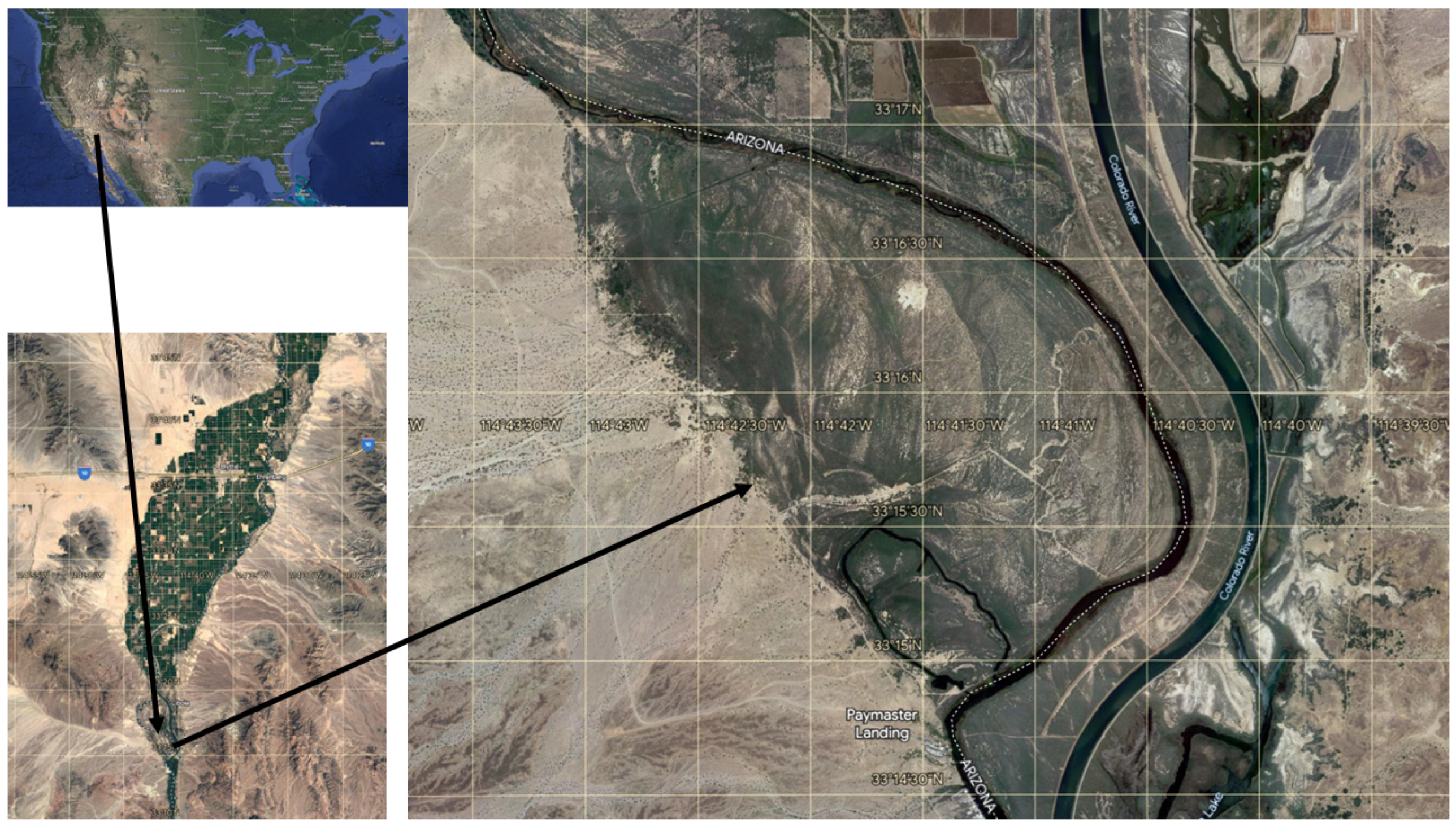
The field experiment was conducted at Cibola National Wildlife Refuge (CNWR) in the southwestern United States, both on the California side at the California–Arizona boundary (Figure 1). CNWR is located within the Sonoran Desert region in the southwestern United States, that has an extreme arid climatic condition. CNWR receives very low precipitation with an annual mean of about 100 mm. The soil is predominantly sandy and silt loam, with little clay. The soil is basic in nature (pH > 8), with a high percentage of salt (NaCl). The soil salinity gradually increases with distance from the Lower Colorado River [45].

2.2. Bowen Ratio Data Collection

CNWR, was primarily dominated by dense patches of salt cedar. Three Bowen ratio energy balance (BREB) towers were installed inside CNWR, with increasing distance from the Lower Colorado river. The BREB tower closest to the Lower Colorado river was in swamp. The next BREB tower was installed a little further from the river within a dense patch of salt cedar and was named Slytherin, and the one farthest from the river was named Diablo. The swamp site soil was a little moist from the nearby river (swampy) and in a bare spot nearby, though in general the vegetation was healthy. Slytherin was located within a dense patch of salt cedar. Near the Diablo site the vegetation was a little stressed due to the soil salinity [46].

The BREB towers were purchased from Radiation and Energy Balance Inc. (Pullman, WA, USA). The BREB towers were primarily assemblages of several weather sensors installed at specific locations. The net radiation ($R_n$) was calculated as energy balance between incoming and outgoing shortwave and longwave radiation. The net radiation was measured at an adequate height above the canopies to cover all plants within the footprint. One temperature ($t$) and one vapor pressure ($vp$) sensor each was placed within the same hollow cylinder, and two such cylinders were installed above the plant canopies, to be above the boundary layer, vertically separated by one meter. The differences in temperatures ($∆t$) and vapor pressures ($∆vp$) were required to estimate ET. The cylinders interchanged their positions at 15-min intervals to avoid any position bias. Soil heat flux ($G$) sensors were placed within 5 cm of the soil surface. The energy balance equation plays a significant role in estimating ET by the Bowen ratio method. The mathematical representation of the energy balance equation is [23]:

$$\mathsf{\lambda }\mathrm{E}\mathrm{T}={\mathrm{R}}_{\mathrm{n}}-\mathrm{G}-\mathrm{H}$$

(1)

The ET by the Bowen ratio method was calculated as [18]:

$$\mathrm{E}\mathrm{T}=\frac{{\mathrm{R}}_{\mathrm{n}}-\mathrm{G}}{1+\frac{\mathrm{H}}{\mathsf{\lambda }\mathrm{E}\mathrm{T}}}=\frac{{\mathrm{R}}_{\mathrm{n}}-\mathrm{G}}{1+\mathsf{\gamma }\frac{∆\mathrm{t}}{∆\mathrm{v}\mathrm{p}}}$$

(2)

where $\gamma$ is called the psychrometric constant.

Salt cedars are tall crops, occasionally reaching up to 20 feet in height. To measure ET accurately, it is important that the BREB sensors placed above the crop canopies. Swamp, Slytherin, and Diablo were installed on top of scaffoldings, tall enough so that the BREB towers appeared to be installed above the canopies. Swamp and Slytherin were installed during the early spring of 2007, and Diablo was installed during the early spring of 2008. Thus, Swamp, and Slytherin collected data over the entire growing seasons of 2007 and 2008, while Diablo collected data over the growing season of 2008. The BREB systems measured ET data in units of energy W m⁻² every 15-min, which were converted into units of water loss per squared-meter (reverse rain) and were summed to measure total daily ET in units of mm d⁻¹. Finally, the data were so arranged that Swamp, and Slytherin had equal an number of observations with 2007 and 2008 data combined [46].

2.3. Collection of Remote Sensing Data

2.3.1. Enhanced Vegetation Indices

Moderate Resolution Imaging Spectroradiometer (MODIS) derived Enhanced Vegetation Indices (EVI) images for growing the seasons of 2007 and 2008 were collected from the United States Geological Survey’s EROS Data Center (Sioux Falls, SD, USA). EVI was an improvement over the Normalized Difference Vegetation Index (NDVI), calculated from reflectance of near-infrared (${\mathsf{\rho }}_{\mathrm{N}\mathrm{I}\mathrm{R}}$), red (${\mathsf{\rho }}_{\mathrm{R}}$), and blue (${\mathsf{\rho }}_{\mathrm{B}}$) light by plant canopies as previously described [47,48]:

$$\mathrm{E}\mathrm{V}\mathrm{I}=2.5\frac{{\mathsf{\rho }}_{\mathrm{N}\mathrm{I}\mathrm{R}}-{\mathsf{\rho }}_{\mathrm{R}}}{{\mathsf{\rho }}_{\mathrm{N}\mathrm{I}\mathrm{R}}+6{\mathsf{\rho }}_{\mathrm{R}}-7.5{\mathsf{\rho }}_{\mathrm{B}}+1}$$

(3)

The Terra satellite, hosting the MODIS system had a 16-day repeat time. However, the MODIS system had a large spatial coverage [49], large enough to acquire more than single images per location, and MODIS VI products were the composite images (by picking the best pixels) [48]. MODIS EVI images were available in a binary format, which were reprojected in the UTM zone (NAD-27 datum), and after rejecting everything but the best pixels, EVI values for each tower site were collected for the entire growing seasons of 2007 and 2008. Thus, 16-day EVI values were obtained for each tower site over the entire growing seasons of 2007 and 2008, which were converted to daily EVI via linear interpolation. These EVI values existed between 0 to 1.2, which were further normalized to range between 0 and 1 [46].

2.3.2. Solar Radiation, Surface Temperature, and Relative Humidity

From Equation (2) it was evident that the Bowen ratio method, one way or another, uses net radiation, air temperature, and vapor pressure. There was no known source from where those variables, completely remote sensing based measurements or estimations, would have been available. The closest possible satellite derived variables available were the Global Horizontal Irradiance (GHI), Surface Temperature (TS), and Relative Humidity (RH), from the National Renewable Energy Laboratory (Golden, CO, USA) (NREL) database. GHI data were calculated by combining images from the Geostationary Operational Environmental Satellite (GOES), Modern Era Retrospective analysis for Research and Applications-version 2 (MERRA-2), MODIS, and the Ice Mapping System (IMS), and TS and RH data were calculated from MERRA-2 images [50]. The hourly data of GHI, TS, and RH were collected, from NREL, for the entire growing seasons of 2007 and 2008, and were converted into daily averages, before being used in the models.

2.4. Machine Learning Modeling

Machine learning (ML) is a procedure of learning from observations [51]. Advancement in technologies have initiated a boost in collecting significant amounts of data, which has generated a pool in a large number of databases. The relationships between variables in these large databases are often difficult to explain with traditional hypotheses. ML techniques split these data into training and validation and learn these relationships from the database itself. Training data is used to train the model and validation data is used to validate the model [52]. Many different types of models were tested via ML techniques. Among them, the simplest ones were linear models. Linear models estimate model parameters using least squares estimators. The success of linear models rely on some constant slopes between predictors and responses in both training and validation data [53]. However, often least squares estimators become dependent on training data. To avoid this dependency on training data some validation data biases are often added at the expense of a reduced R² [54,55,56]. For ridge regression, the biases are the sum of the squares of the slopes of predictors, estimated by least squares estimators [54]. For lasso regression the biases are simply the sum of the slopes of the predictors, estimated by least squares estimators [55]. Again, elastic net regression is a “convex combination” of ridge and lasso regression, where both aforementioned types of biases are combined together [56]. It is a modification to multiple regression analysis, where first a principal component analysis is performed on the variables, then the principal components are arranged in descending order, and regression is calculated based on the top principal components [57]. Principal component regression has some added advantages over multiple regression during multicollinearity issues, and works well with smaller samples [58]. In this research, linear (LM), ridge (RR), lasso (LR), elastic net (EN), and principal component regressions (PCR) were applied.

Often, least squares-based estimators fail to generate good predictive models, especially in the presence of spare data. In such cases classification-based regression models might be better options. Decision tree is one such good example of classifiers, where the classification is made based on some rank, which is estimated on some inter-relation within the training data itself [59]. A further modification to decision tree is random forest (RF), where a user classified large number of decision trees are gathered up (and thus named a forest). Though the actual number of trees required are determined by the user, the minimum number of trees required depends on the sparseness in the data [60]. In random forest, the user decides the number of decision trees to be included in the modeling. An advancement of random forest is gradient boosting machine (GBM), where the number of decision trees are estimated based on the model fitting criteria itself [61]. Another improvement of random forest and even of GBM, is extreme gradient boosting (XGBoost). The improvement was made specially to analyze sparse data and to better analyze tree learning [62]. Another type of classifier are support vector machines, which are a set of binary classification-based models [63]. The data is split into two groups (and thus is binary) and separated by a hyperplane, which can be linear, polynomial, or radial [64]. Another type of classifier is a supervised learning method that estimates its learning function based on an input vector and its output from training data, and then estimates the accuracies for validation. To avoid noise, multiple input vectors are often utilized. The selection of input vector can be either by looking at the accuracies of the learning functions within the training dataset, or can be just based on the training dataset itself, completely ignoring the learning functions [65]. In this research RF, GBM, XGBoost, support vector machines with linear (SVM-L), polynomial (SVM-P), and radial (SVM-R) kernel, and k-nearest neighbor estimators (kNN) were tested (Table 1).

In this study 70% of the observations were used for training the models and the rest (30%) for the validation. The machine learning modeling procedures were adopted from [66,67]. A ten-fold cross validation was calculated with five-repetitions, and the model accuracies were estimated by comparing correlations between estimated and predicted estimations of the validation data. The entire procedure (including the cross validation) was repeated 500 times via a “for” loop for each model. For each model, the median values of 500 correlations were compared to identify the optimum model. Additionally, for each median correlation value, the range of accuracies, the maximum and minimum correlation values out of the 500 iterations, were obtained to emphasize the reliability of the model. The entire calculations were performed in R, within the R-Studio environment, applying the following R packages:

Table 1. Regression models and the associated R-packages used.

Regression Models Used	R Packages Used
Linear regression	caret [68]
Lasso regression	caret [68]
Ridge regression	caret [68]
Elastic net regression	caret [68]
Random forest	randomForest [69]
Gradient boosting machine	caret [68]
Extreme gradient boosting	rminer [70]
Support vector machines (all kernels used)	rminer [70]
Principal component regression	pls [58]
k-nearest neighbor	caret [68]

Table 1. Regression models and the associated R-packages used.

Regression Models Used	R Packages Used
Linear regression	caret [68]
Lasso regression	caret [68]
Ridge regression	caret [68]
Elastic net regression	caret [68]
Random forest	randomForest [69]
Gradient boosting machine	caret [68]
Extreme gradient boosting	rminer [70]
Support vector machines (all kernels used)	rminer [70]
Principal component regression	pls [58]
k-nearest neighbor	caret [68]

Several models could be developed using the available predictors. In this research all possible models using those predictors, with EVI being at least one of the predictors, were tested. EVI was the only variable available that represented plant health. Thus, the following models (with four, three, and two predictors) were tested:

Model 1: EVI, GHI, TS and RH as regressors

Model 2: EVI, GHI, and TS as regressors

Model 3: EVI, TS, and RH as regressors

Model 4: EVI, GHI, and RH as regressors

Model 5: EVI and GHI as regressors

Model 6: EVI and TS as regressors

Model 7: EVI and RH as regressors

3. Results

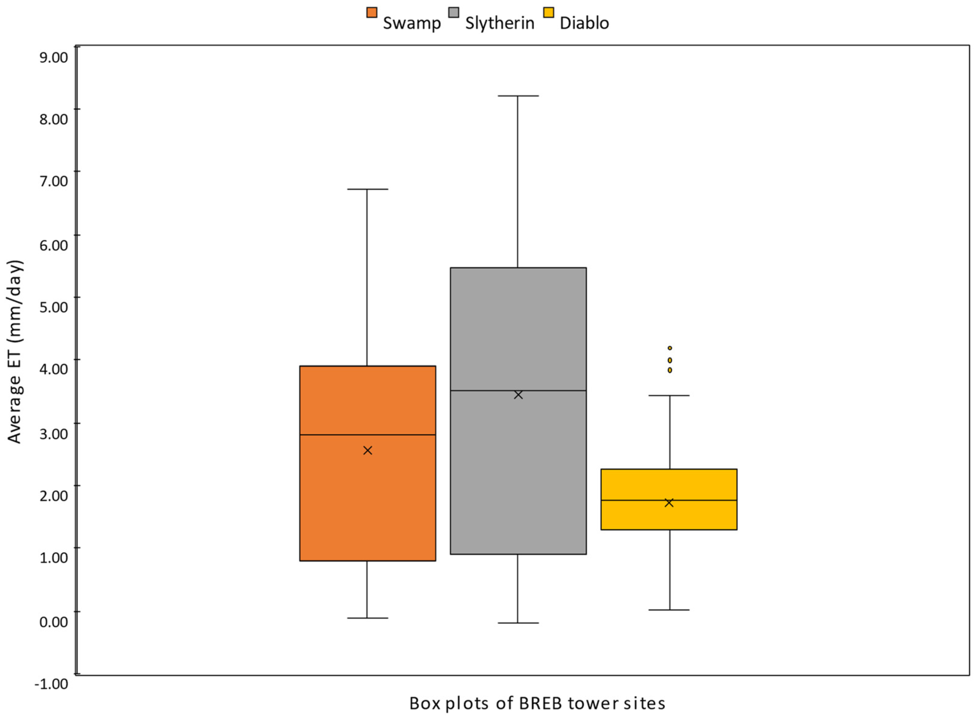
3.1. ET Estimated by BREB Towers

Among the three sites Slytherin measured the highest ET. Slytherin measured maximum daily ET of about 8 mm d⁻¹, Swamp measured maximum daily ET of between 6 and 7 mm d⁻¹, and Diablo measured a maximum daily ET of between 3 and 4 mm d⁻¹, with their respective averages 3–4 mm d⁻¹, 3–4 mm d⁻¹, and 2–3 mm d⁻¹ (Figure 2 and Figure 3).

3.2. Accuracies Produced by Different Models

All the machine learning results have been summarized in

Table 2. Results of the machine learning modeling. Median (Med), minimum (Min), maximum (Max) of correlations have been shown against different models tested.

Models	STAT	EN	GBM	KNN	LASSO	PCR	RF	RIDGE	SVM-L	SVM-P	SVM-R	XGBOOST
	Med	90	94	85	90	90	94	94	90	90	93	92
Model-1	Min	89	92	81	89	88	92	92	89	89	91	91
	Max	92	95	88	92	92	95	95	92	92	94	94
	Med	90	93	85	90	90	94	90	90	90	93	92
Model-2	Min	89	92	81	88	87	92	88	88	88	91	90
	Max	92	95	89	92	92	96	92	92	92	95	94
	Med	87	91	82	87	87	92	87	87	87	90	90
Model-3	Min	84	89	78	85	84	89	84	85	85	87	86
	Max	90	93	86	90	90	94	90	90	90	93	92
	Med	89	92	76	89	89	92	89	89	89	92	91
Model-4	Min	86	89	71	86	86	90	86	86	86	89	88
	Max	91	94	80	91	91	94	91	91	91	93	93
	Med	89	92	76	89	89	92	89	89	89	91	91
Model-5	Min	86	89	69	86	86	89	86	86	86	89	89
	Max	91	93	81	91	91	94	91	91	91	94	93
	Med	87	91	82	87	87	92	87	87	87	90	90
Model-6	Min	84	89	78	85	84	89	84	85	85	87	86
	Max	90	93	86	90	90	94	90	90	90	93	92
	Med	87	91	85	87	87	91	87	87	87	89	89
Model-7	Min	85	88	82	85	85	89	85	85	85	86	87
	Max	89	93	88	89	89	93	89	89	89	92	92

. Among all the regression types tested during the machine learning algorithms, random forest consistently produced the best accuracies for all the models. Model 1 and Model 2 produced the maximum accuracy (94%) using the random forest. For other models, accuracies produced by random forest ranged between 91 and 92%, where 91% accuracy was observed for Model 7 only. Again, for Model 4 both GBM and SVM-R produced maximum accuracies, with RF. For any other model types GBM, SVM-R, and XGBoost produced consistently high accuracies, but not the maximum. All other regression types produced maximum accuracies for all models, ranging between 87 and 90%. Only kNN produced consistently poor accuracies for all models. Additionally, the difference between maximum and minimum accuracies produced by kNN were consistently higher than any other regression type, indicating higher variance.

Model 1 produced maximum accuracies, in the range of 93–94%, while using GBM, RF, RR, and SVM-R. Further, GBM, RF, and SVM-R of Model 2 produced similar accuracies. Among Models 2–4, Model 2 regressions produced overall higher accuracies. Only RF produced accuracies in the range of 91–92% for other models. Among Models 5–7, Model 5 produced overall higher accuracies. GBM, RF, SVM-R, and XGBoost produced accuracies within the range of 91–92%, while others (except kNN) produced an accuracy of 89%.

4. Discussions

ET is a combined effect of environment, plant growth and health conditions. Thus, any good ET estimating model, for estimating ET from a large spatial region, should include variables representing environment, and plant growth and plant health. Accordingly, GHI, TS, and RH represent environmental conditions, and EVI represents plant growth and health conditions. Among all the models tested Model 1, Models 2–4, and Models 5–7 can be grouped into three categories. Model 1 uses all the four variables as predictors. The second group uses EVI and a combination of two out of three environmental variables, as predictors. The third group uses EVI and a combination of one out of three environmental variables, as predictors. Thus, this research examined experimentally all possible scenarios involving remote sensing-based ET estimations using the predictors used in this research.

Among all the regression types tested, RF consistently produced higher accuracies among all of them. For example, for Model 1 and 2, RF produced accuracies of about 94%. Even the lowest accuracies produced by RF were about 91% for Model 7. For the rest of the models RF produced accuracies of about 92%. After RF, XGBoost, GBM, and SVM-R, consistently, produced the second highest accuracies, between about 89 and 92%. For Model 1 XGBoost, GBM, and SVM-R produced accuracies that were even as good as RF. kNN consistently produced the poorest accuracies among all the regression types. Even maximum accuracies produced by kNN were 85%, for Model 1. The rest of the regression types produced accuracies of about 87–90% for all the models.

The most important outcome was that remote sensing based models were able to estimate ET with high accuracies. According to this research, if random forest is used to generate the models, remote sensing-based RH turned out to be the least important variable. This explains how Model 1 (where EVI, GHI, TS, and RH were the predictors) and Model 2 (where EVI, GHI, and TS were the predictors) produced the same high accuracies. Again, if only one predictor, other than EVI, can be used, GHI is the most important variable. Finally random forest turned out to be the most important modeling procedure.

To implement this workflow in practice, a simple modification to the suggested procedure may be necessary. The workflow can be summarized as follows:

For implementing these methods, it is recommended to install and maintain, in-field ET estimating systems, preferably one each at each distinguishably different vegetation types/conditions. For example, in this study, a swampy zone with a bare spot (Swamp), dense vegetation (Slytherin), and salinity stressed (Diablo) vegetative locations were selected. ET should be measured for a few seasons/years initially, which can be considered as the “training period”.

Remote sensing based EVI, GHI, TS, RH data should be collected for the footprint pixels of the in-field ET measurement locations, for the training period.

Optimum models must be generated following the machine learning algorithm. R-codes for running the machine learning analysis can be made available via GitHub, if requested.

For the time frame for which ET needs to be estimated at a regional scale (can be considered the “implementation period”) EVI, GHI, TS, RH data should be collected for the entire region of interest (for example, for this study the entire CNWR region).

Re-run the algorithms of the optimum model decided on after step 3, only this time all training period data should be used, and only one iteration should be made.

The end product after step 5, will provide ET for the entire region.

For best results, it would be recommended to repeat the entire procedure, preferably every growing season, or at least frequently, to modify model parameters.

5. Conclusions

The aim of this study was to generate models to precisely estimate ET over large regions. The preliminary model, which used EVI, GHI, TS, and RH as predictors, produced the best accuracies from 92 to 94% using everything but the kNN procedure, and about 85% using kNN. This model used all the variables, or their close relatives, that BREB towers used. However, other simpler models, using EVI, GHI, and TS, also produced similar accuracies (92–94%) while using random forest, gradient boosting machine, extreme gradient boosting, and support vector machine with radial kernel. Thus, these two models can be used as optimum models. Apart from the above, this study revealed some other important outcomes. First, though the models were developed based on data from three or four BREB tower sites, the models could be easily scaled over a large spatial region. The workflow for this scale conversion has also been briefly described in the “Discussion” section.

The modeling approach suggested that if the data set can be grouped into several levels based on its average values, classification-based methods, such as random forest, gradient boosting machine, extreme gradient boosting, support vector machine, etc. work better than correlation-based methods such as linear models, ridge, lasso, or elastic net regressions. For this dataset however, random forest performed better, for other datasets other classification-based model types (e.g., support vector machine) may also be worthwhile investigating.

References

- Jacobs, J.; Sing, S. Ecology and Management of Saltcedar (Tamarix ramosissima, T. chinensis and T. ramosissima × T. chinensis Hybrids); Invasive Species Technical Note No. MT-13; U.S. Department of Agriculture, Natural Resources Conservation Service: Bozeman, MT, USA, 2007; 12p. [Google Scholar]
- Natale, E.; Zalba, S.M.; Oggero, A.; Reinoso, H. Establishment of Tamarix ramosissima under different conditions of salinity and water availability: Implications for its management as an invasive species. J. Arid. Environ. 2010, 74, 1399–1407. [Google Scholar] [CrossRef]
- Everitt, B.L. Ecology of saltcedar—A plea for research. Environ. Geol. 1980, 3, 77–84. [Google Scholar] [CrossRef]
- Nagler, P.L.; Hinojosa-Huerta, O.; Glenn, E.P.; Garcia-Hernandez, J.; Romo, R.; Curtis, C.; Huete, A.R.; Nelson, S.G. Regeneration of native trees in the presence of invasive Saltcedar in the Colorado river delta, Mexico. Conserv. Biol. 2005, 19, 1842–1852. [Google Scholar] [CrossRef]
- Blaney, H.F.; Criddle, W.D. Determining Consumptive Use and Irrigation Water Requirements; US Department of Agriculture: Bozeman, MT, USA, 1962. [Google Scholar]
- Yu, T.; Qi, F.; Si, J.; Zhang, X.; Zhao, C. Tamarix ramosissima stand evapotranspiration and its association with hydroclimatic factors in an arid region in northwest China. J. Arid Environ. 2017, 138, 18–26. [Google Scholar] [CrossRef]
- Nagler, P.L.; Morino, K.; Didan, K.; Erker, J.; Osterberg, J.; Hultine, K.R.; Glenn, E.P. Wide-area estimates of saltcedar (Tamarix spp.) evapotranspiration on the lower Colorado River measured by heat balance and remote sensing methods. Ecohydrology 2009, 2, 18–33. [Google Scholar] [CrossRef]
- Davenport, D.C.; Martin, P.E.; Hagan, R.M. Evapotranspiration from riparian vegetation: Water relations and irrecoverable losses for saltcedar. J. Soil Water Conserv. 1982, 37, 233. [Google Scholar]
- Cleverly, J.R.; Dahm, C.N.; Thibault, J.R.; McDonnell, D.E.; Allred Coonrod, J.E. Riparian ecohydrology: Regulation of water flux from the ground to the atmosphere in the Middle Rio Grande, New Mexico. Hydrol. Process. 2006, 20, 3207–3225. [Google Scholar] [CrossRef]
- Devitt, D.A.; Salal, A.; Mace, K.A.; Smith, S.D. The effect of applied water on the water use of saltcedar in a desert riparian environment. J. Hydrol. 1997, 192, 233–246. [Google Scholar] [CrossRef]
- Westenburg, C.L.; Harper, D.P.; DeMeo, G.A. Evapotranspiration by Phreatophytes along the Lower Colorado River at Havasu National Wildlife Refuge, Arizona; Scientific Investigations Report; USGS: Reston, VA, USA, 2006; p. 44. [Google Scholar]
- Sala, A.; Smith, S.D.; Devitt, D.A. Water use by Tamarix ramosissima and associated phreatophytes in a Mojave desert floodplain. Ecol. Appl. 1996, 6, 888–898. [Google Scholar] [CrossRef]
- Swinbank, W.C. The measurement of vertical transfer of heat and water vapor by eddies in the lower atmosphere. J. Atmos. Sci. 1951, 8, 135–145. [Google Scholar] [CrossRef]
- Bowen, I.S. The Ratio of Heat Losses by Conduction and by Evaporation from any Water Surface. Phys. Rev. 1926, 27, 779–787. [Google Scholar] [CrossRef]
- Monteith, J.L. Evaporation and environment. Symp. Soc. Exp. Biol. 1965, 19, 205–234. [Google Scholar]
- Penman, H.L. Evaporation an Introductory Survey. Neth. J. Agric. Sci. 1956, 4, 9–29. [Google Scholar] [CrossRef]
- Allen, R.G.; Pereira, L.S.; Smith, M.; Raes, D.; Wright, J.L. FAO-56 Dual Crop Coefficient Method for Estimating Evaporation from Soil and Application Extensions; FAO: Rome, Italy, 2005. [Google Scholar]
- Allen, R.G.; Pruitt, W.O.; Businger, J.A.; Fritschen, F.J.; Jensen, M.E.; Quinn, F.H. Chapter 4, Evaporation and Transpiration. In Hydrology Handbook; Heggen, R.J., Ed.; American Society of Civil Engineers: Reston, VA, USA, 1996. [Google Scholar]
- Davie, T.; Quinn, N.W. Fundamentals of Hydrology; Routledge: Informa, UK, 2019. [Google Scholar]
- Rana, G.; Katerji, N. Measurement and estimation of actual evapotranspiration in the field under Mediterranean climate: A review. Eur. J. Agron. 2000, 13, 125–153. [Google Scholar] [CrossRef]
- Smith, D.M.; Allen, S.J. Measurement of sap flow in plant stems. J. Exp. Bot. 1996, 47, 1833–1844. [Google Scholar] [CrossRef]
- Giménez, C.; Gallardo, M.; Thompson, R.B. Plant–Water Relations. In Reference Module in Earth Systems and Environmental Sciences; Elsevier: Amsterdam, The Netherlands, 2013. [Google Scholar] [CrossRef]
- Li, Z.-L.; Ronglin, T.; Zhengming, W.; Yuyun, B.; Chenghu, Z.; Bohui, T.; Guangjian, Y.; Xiaoyu, Z. A Review of Current Methodologies for Regional Evapotranspiration Estimation from Remotely Sensed Data. Sensors 2009, 9, 3801–3853. [Google Scholar] [CrossRef]
- Justice, C.O.; Townshend, J.R.G.; Vermote, E.F.; Masuoka, E.; Wolfe, R.E.; Saleous, N.; Roy, D.P.; Morisette, J.T. An overview of MODIS Land data processing and product status. Remote Sens. Environ. 2002, 83, 3–15. [Google Scholar] [CrossRef]
- Acharya, T.D.; Yang, I. Exploring landsat 8. Int. J. IT Eng. Appl. Sci. Res. 2015, 4, 4–10. [Google Scholar]
- Bastiaanssen, W.G.; Menenti, M.; Feddes, R.; Holtslag, A. A remote sensing surface energy balance algorithm for land (SEBAL). 1. Formulation. J. Hydrol. 1998, 212, 198–212. [Google Scholar] [CrossRef]
- Allen, R.G.; Tasumi, M.; Trezza, R. Satellite-based energy balance for mapping evapotranspiration with internalized calibration (METRIC)—Model. J. Irrig. Drain. Eng. 2007, 133, 380–394. [Google Scholar] [CrossRef]
- Roerink, G.; Su, Z.; Menenti, M. S-SEBI: A simple remote sensing algorithm to estimate the surface energy balance. Phys. Chem. Earth Part B Hydrol. Ocean. Atmos. 2000, 25, 147–157. [Google Scholar] [CrossRef]
- Norman, J.M.; Kustas, W.P.; Humes, K.S. Source approach for estimating soil and vegetation energy fluxes in observations of directional radiometric surface temperature. Agric. For. Meteorol. 1995, 77, 263–293. [Google Scholar] [CrossRef]
- Mecikalski, J.R.; Mackaro, S.M.; Anderson, M.C.; Norman, J.M.; Basara, J.B. Evaluating the use of the Atmospheric Land Exchange Inverse (ALEXI) model in short-term prediction and mesoscale diagnosis. In Proceedings of the Conference on Hydrology, San Diego, CA, USA, 7–9 May 2015; pp. 8–13. [Google Scholar]
- Su, Z. The Surface Energy Balance System (SEBS) for estimation of turbulent heat fluxes. Hydrol. Earth Syst. Sci. 2002, 6, 85–100. [Google Scholar] [CrossRef]
- Glenn, E.P.; Huete, A.R.; Nagler, P.L.; Hirschboeck, K.K.; Brown, P. Integrating remote sensing and ground methods to estimate evapotranspiration. Crit. Rev. Plant Sci. 2007, 26, 139–168. [Google Scholar] [CrossRef]
- Nagler, P.L.; Morino, K.; Murray, R.S.; Osterberg, J.; Glenn, E.P. An Empirical Algorithm for Estimating Agricultural and Riparian Evapotranspiration Using Modis Enhanced Vegetation Index and Ground Measurements of E. T. I. Description of Method. Remote Sens. 2009, 1, 1273–1297. [Google Scholar] [CrossRef]
- Jiang, L.; Islam, S. A methodology for estimation of surface evapotranspiration over large areas using remote sensing observations. Geophys. Res. Lett. 1999, 26, 2773–2776. [Google Scholar] [CrossRef]
- Moran, M.S.; Clarke, T.R.; Inoue, Y.; Vidal, A. Estimating crop water deficit using the relation between surface-air temperature and spectral vegetation index. Remote Sens. Environ. 1994, 49, 246–263. [Google Scholar] [CrossRef]
- Nagler, P.; Jetton, A.; Fleming, J.; Didan, K.; Glenn, E.; Erker, J.; Morino, K.; Milliken, J.; Gloss, S. Evapotranspiration in a cottonwood (Populus fremontii) restoration plantation estimated by sap flow and remote sensing methods. Agric. For. Meteorol. 2007, 144, 95–110. [Google Scholar] [CrossRef]
- Maeda, E.E.; Wiberg, D.A.; Pellikka, P.K.E. Estimating reference evapotranspiration using remote sensing and empirical models in a region with limited ground data availability in Kenya. Appl. Geogr. 2011, 31, 251–258. [Google Scholar] [CrossRef]
- Mosre, J.; Suárez, F. Actual evapotranspiration estimates in arid cold regions using machine learning algorithms with in situ and remote sensing rata. Water 2021, 13, 870. [Google Scholar] [CrossRef]
- Ray, S.S.; Dadhwal, V.K. Estimation of crop evapotranspiration of irrigation command area using remote sensing and GIS. Agric. Water Manag. 2001, 49, 239–249. [Google Scholar] [CrossRef]
- Pereira, L.S.; Allen, R.G.; Smith, M.; Raes, D. Crop evapotranspiration estimation with FAO56: Past and future. Agric. Water Manag. 2015, 147, 4–20. [Google Scholar] [CrossRef]
- Kullberg, E.G.; DeJonge, K.C.; Chávez, J.L. Evaluation of thermal remote sensing indices to estimate crop evapotranspiration coefficients. Agric. Water Manag. 2017, 179, 64–73. [Google Scholar] [CrossRef]
- Wang, J.; Sammis, T.W.; Gutschick, V.P.; Gebremichael, M.; Miller, D.R. Sensitivity Analysis of the Surface Energy Balance Algorithm for Land (SEBAL). Trans. ASABE 2009, 52, 801–811. [Google Scholar] [CrossRef]
- Long, D.; Singh, V.P.; Li, Z.-L. How sensitive is SEBAL to changes in input variables, domain size and satellite sensor? J. Geophys. Res. Atmos. 2011, 116, D21. [Google Scholar] [CrossRef]
- Mokhtari, M.; Ahmad, B.; Hoveidi, H.; Busu, I. Sensitivity analysis of METRIC–based evapotranspiration algorithm. Int. J. Environ. Res. 2013, 7, 407–422. [Google Scholar]
- Glenn, E.P.; Morino, K.; Nagler, P.L.; Murray, R.S.; Pearlstein, S.; Hultine, K.R. Roles of saltcedar (Tamarix spp.) and capillary rise in salinizing a non-flooding terrace on a flow-regulated desert river. J. Arid Environ. 2012, 79, 56–65. [Google Scholar] [CrossRef]
- Chatterjee, S. Estimating Evapotranspiration Using Remote Sensing: A Hybrid Approach between MODIS Derived Enhanced Vegetation Index, Bowen Ratio System, and Ground Based Micro-Meteorological Data. Ph.D. Thesis, Wright State University, Dayton, OH, USA, 2010. [Google Scholar]
- Huete, A.; Didan, K.; Miura, T.; Rodriguez, E.P.; Gao, X.; Ferreira, L.G. Overview of the radiometric and biophysical performance of the MODIS vegetation indices. Remote Sens. Environ. 2002, 83, 195–213. [Google Scholar] [CrossRef]
- Huete, A.J.C. MODIS vegetation index (MOD13). In Algorithm Theoretical Basis Documents; University of Arizona & University of Virginia: Tucson, AZ, USA, 1999. [Google Scholar]
- Pagano, T.S.; Durham, R.M. Moderate resolution imaging spectroradiometer (MODIS). In Sensor Systems for the Early Earth Observing System Platforms; SPIE: Bellingham, WA, USA, 1993; pp. 2–17. [Google Scholar]
- Sengupta, M.; Xie, Y.; Lopez, A.; Habte, A.; Maclaurin, G.; Shelby, J. The National Solar Radiation Data Base (NSRDB). Renew. Sustain. Energy Rev. 2018, 89, 51–60. [Google Scholar] [CrossRef]
- Mitchell, T.; Buchanan, B.; DeJong, G.; Dietterich, T.; Rosenbloom, P.; Waibel, A. Machine learning. Annu. Rev. Comput. Sci. 1990, 4, 417–433. [Google Scholar] [CrossRef]
- Vabalas, A.; Gowen, E.; Poliakoff, E.; Casson, A.J. Machine learning algorithm validation with a limited sample size. PLoS ONE 2019, 14, e0224365. [Google Scholar] [CrossRef] [PubMed]
- Maulud, D.; Abdulazeez, A.M. A review on linear regression comprehensive in machine learning. J. Appl. Sci. Technol. Trends 2020, 1, 140–147. [Google Scholar] [CrossRef]
- Hoerl, A.E.; Kennard, R.W. Ridge Regression: Biased Estimation for Nonorthogonal Problems. Technometrics 1970, 12, 55–67. [Google Scholar] [CrossRef]
- Tibshirani, R. Regression Shrinkage and Selection via the Lasso. J. R. Stat. Soc. Ser. B 1996, 58, 267–288. [Google Scholar] [CrossRef]
- García-Nieto, P.J.; García-Gonzalo, E.; Paredes-Sánchez, J.P. Prediction of the critical temperature of a superconductor by using the WOA/MARS, Ridge, Lasso and Elastic-net machine learning techniques. Neural Comput. Appl. 2021, 33, 17131–17145. [Google Scholar] [CrossRef]
- Mevik, B.-H.A.W.R. The pls Package: Principal Component and Partial Least Squares Regression in R. J. Stat. Softw. 2007, 18, 1–23. [Google Scholar] [CrossRef]
- Hovde Liland, K.; Mevik, B.-H.; Wehrens, R. Pls: Partial Least Squares and Principal Component Regression. R Package Version 2.8-1. 2022. Available online: https://analyticalsciencejournals.onlinelibrary.wiley.com/doi/10.1002/cem.873 (accessed on 10 October 2023).
- Myles, A.J.; Feudale, R.N.; Liu, Y.; Woody, N.A.; Brown, S.D. An introduction to decision tree modeling. J. Chemom. 2004, 18, 275–285. [Google Scholar] [CrossRef]
- Breiman, L. Random Forests. Mach. Learn. 2004, 45, 5–32. [Google Scholar] [CrossRef]
- Jerome, H.F. Greedy function approximation: A gradient boosting machine. Ann. Stat. 2001, 29, 1189–1232. [Google Scholar] [CrossRef]
- Chen, T.; Guestrin, C. XGBoost: A Scalable Tree Boosting System. In Proceedings of the 22nd ACM SIGKDD International Conference on Knowledge Discovery and Data Mining, San Francisco, CA, USA, 13–17 August 2016. [Google Scholar]
- Todorov, K.; Geibel, P.; K¨uhnberger, K.-U. Mining concept similarities for heterogeneous ontologies. In Advances in Data Mining-Applications and Theoretical Aspects; 10th Industrial Conference, ICDM 2010, Proceedings; Goebel, R., Siekmann, J., Wahlster, W., Eds.; Springer: Berlin/Heidelberg, Germany, 2010; pp. 86–100. [Google Scholar]
- Wang, P.; Mao, G. Describing data with the support vector shell in distributed environments. In Advances in Data Mining-Applications and Theoretical Aspects; Goebel, R., Siekmann, J., Wahlster, W., Eds.; Springer: Berlin/Heidelberg, Germany, 2010; pp. 128–142. [Google Scholar]
- Song, Y.; Liang, J.; Lu, J.; Zhao, X. An efficient instance selection algorithm for k nearest neighbor regression. Neurocomputing 2017, 251, 26–34. [Google Scholar] [CrossRef]
- Adak, A.; Murray, S.C.; Božinović, S.; Lindsey, R.; Nakasagga, S.; Chatterjee, S.; Anderson, S.L.; Wilde, S. Temporal vegetation indices and plant height from remotely sensed imagery can predict grain yield and flowering time breeding value in maize via machine learning regression. Remote Sens. 2021, 13, 2141. [Google Scholar] [CrossRef]
- Chatterjee, S.; Adak, A.; Wilde, S.; Nakasagga, S.; Murray, S.C. Cumulative temporal vegetation indices from unoccupied aerial systems allow maize (Zea mays L.) hybrid yield to be estimated across environments with fewer flights. PLoS ONE 2023, 18, e0277804. [Google Scholar] [CrossRef] [PubMed]
- Kuhn, M. Caret: Classification and Regression Training. R Package Version 6.0-93. 2022. Available online: https://cran.r-project.org/web/packages/caret/caret.pdf (accessed on 10 October 2023).
- Liaw, A.; Wiener, M. Classification and regression by randomForest. R News 2022, 2, 18–22. [Google Scholar]
- Cortez, P. Rminer: Data Mining Classification and Regression Methods. R Package Version 1.4.6. 2020. Available online: https://cran.r-project.org/web/packages/rminer/rminer.pdf (accessed on 10 October 2023).