Boundary-Aware Deformable Spiking Neural Network for Hyperspectral Image Classification

Abstract

A few spiking neural network (SNN)-based classifiers have been proposed for hyperspectral images (HSI) classification to alleviate the higher computational energy cost problem. Nevertheless, due to the lack of ability to distinguish boundaries, the existing SNN-based HSI classification methods are very prone to falling into the Hughes phenomenon. The confusion of the classifier at the class boundary is particularly obvious. To remedy these issues, we propose a boundary-aware deformable spiking residual neural network (BDSNN) for HSI classification. A deformable convolution neural network plays the most important role in realizing the boundary-awareness of the proposed model. To the best of our knowledge, this is the first attempt to combine the deformable convolutional mechanism and the SNN-based model. Additionally, spike-element-wise ResNet is used as a fundamental framework for going deeper. A temporal channel joint attention mechanism is introduced to filter out which channels and times are critical. We evaluate the proposed model on four benchmark hyperspectral data sets—the IP, PU, SV, and HU data sets. The experimental results demonstrate that the proposed model can obtain a comparable classification accuracy with state-of-the-art methods in terms of overall accuracy (OA), average accuracy (AA), and statistical kappa ($\kappa$) coefficient. The ablation study results prove the effectiveness of the introduction of the deformable convolutional mechanism for BDSNN’s boundary-aware characteristic.

1. Introduction

Hyperspectral images contain much spectral-spatial information, with hundreds of narrow continuous bands. The significant value of the abundant information they carry has been more and more obvious in many fields, such as agricultural applications [1], geological exploration and mineralogy [2,3], forestry and environmental management [4,5], water and marine resources management [6], and military and defense applications [7,8]. Since HSI classification is one of the most essential procedures of HSI analysis, the innovation discovery in HSI classification has been an increasingly important promotion of the development of these fields mentioned above.

The main task of HSI classification is to label every image pixel based on the feature information carried by the training samples. Many pixel-wise-based HSI classification methods have been proposed based on the realistic idea that different categories of pixels should take different spectral information. For example, methods such as support vector machine (SVM) [9], random forests (RF) [10], and traditional distance metrics-based classifiers [11] treat a single pixel with several bands as a single sample. This view makes them only use spectral information for classification and neglect the rich spatial characteristics. Furthermore, since the features of pixels vary in the same class and resemble the different classes, which is called the salt-and-pepper noise problem, the aforementioned traditional machine learning algorithms can hardly achieve a desirable accuracy.

In recent decades, deep learning (DL) has shown great potential in natural language processing, computer vision, and object detection. In this context, DL-based classifiers, especially convolution neural networks (CNNs)-based approaches, could effectively utilize spatial-spectral information for HSI classification [12,13]. Chen et al. [14] proposed a 2D CNN stacked autoencoder and introduced the CNNs-based method to HSI classification for the first time. Furthermore, to achieve more efficient extractions of spatial-spectral features, the structure of the DL-based model is increasingly complicated, and the number of parameters of the models is increasingly enormous. Roy et al. [15] constructed a hybrid 2D–3D CNN to classify HSI. Hamida et al. [16] used a 3D CNN model to obtain even better classification results. Zhao et al. [17] proposed a convolutional transformer network, which introduced the promising transformer to HSI classification. To ensure that a deeper network achieves better effectiveness, researchers introduced the residual structure into HSI classification [18,19,20]. With the classification model becoming more complex and deeper, and the training and inference time increasing, the computational energy required also increases.

In the past few years, we are rapidly reaching a point where DL may no longer be feasible, while spiking neural networks are one of the most promising paradigms to cross it. Unlike artificial neural networks (ANNs), SNNs use spike sequences to represent information and take advantage of spatiotemporal information during training and inference. Inspired by biological neural networks, the spiking neurons, foundational components of SNN, will remain silent outside of a few active states. Because of the inherent asynchrony and sparseness of spike trains, SNN has the potential to reduce power consumption while maintaining a relatively good performance [21]. Due to the discontinuity of spike trains, to obtain a high-performance SNN, the selection of training methods is the first issue to consider. The current mainstream SNN training methods are divided into ANN to SNN conversion (ANN2SNN) [22] and backpropagation with surrogate gradient [23]. The ANN2SNN method trains an ANN and saves its parameters first, then converts it into an SNN by replacing the activation function with spiking neurons. However, to obtain an accuracy that matches the original ANN, a large timestep is needed for the converted SNN. This limitation causes a counteraction to the low latency characteristics of SNN. The surrogate gradient method achieves error backpropapgation by keeping the non-differentiable firing function in the forward and substituting it with a continuous and smooth surrogate function in the backward. Moreover, the surrogate method can gobtainet direct training SNNs, which could surpass ANNs with similar architecture in an end-to-end manner.

On this basis, many mechanisms and model schemes that have been proven helpful in ANN were introduced into direct training SNN. Fang et al. [24] use the idea of spike-element-wise (SEW) to introduce ResNet into SNN, which makes it possible to achivee a deeper SNN. Zhu et al. [25] proposed a temporal-channel joint attention (TCJA) mechanism and designed an SNN that carried out the weight allocation of time and channel joint information. With these developments, SNN models have achieved noteworthy results in many fields, especially image classification. In recent years, a few researchers have also tried to construct an SNN model to achieve HSI classification. Datta et al. [26] proposed a quantization-aware gradient descent method to train an SNN generated from iso-architecture CNNs for HSI classification. Liu et al. [27,28] proposed two SNN classifiers based on channel shuffle attention mechanisms with two different derivative algorithms. These SNN models for HSI classification tend to fall into the trap of the Hughes phenomenon with fewer training samples. In particular, through there are plenty of experiments for these methods, we found that the pixels on the edges of different categories are most likely to obtain the wrong label, which plays a major role in the causes of the Hughes phenomenon. These issues indicate the limitations of the existing SNN methods for boundary discrimination.

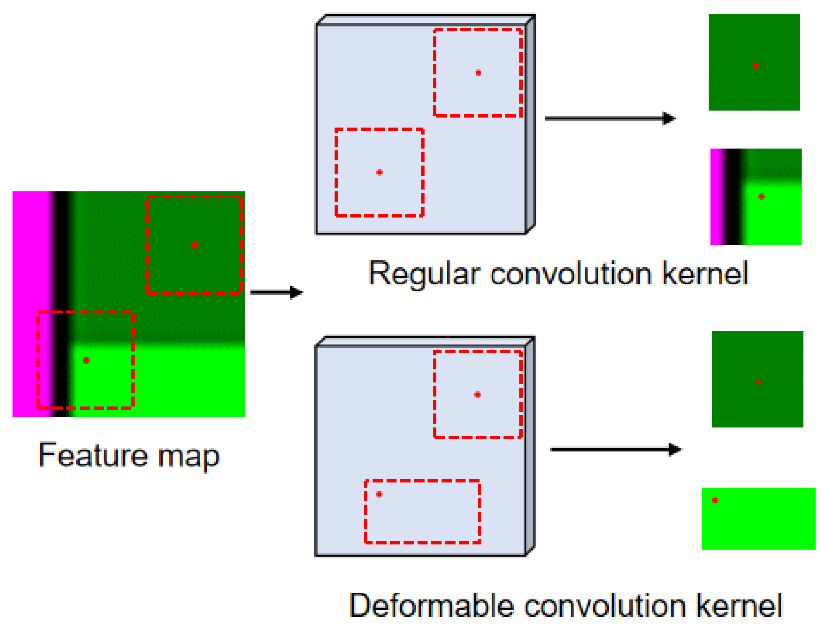
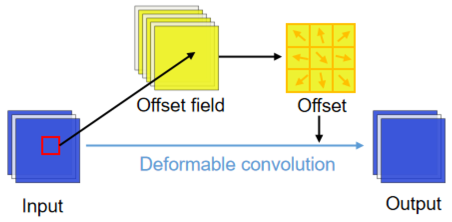
To address the above issues, inspired by the deformable convolutional mechanism [29] in computer vision tasks to distinguish ambiguous boundaries, we proposed a boundary-aware deformable spiking neural network (BDSNN). The contributions of this article are as follows:

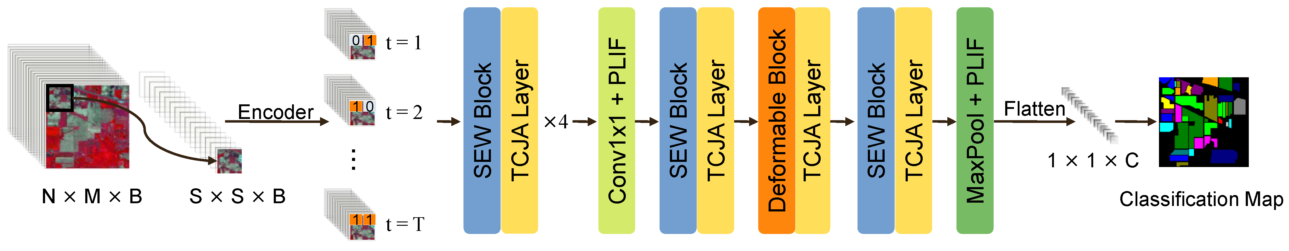
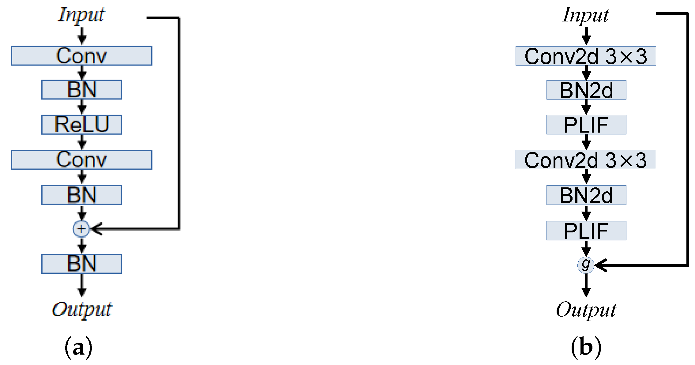
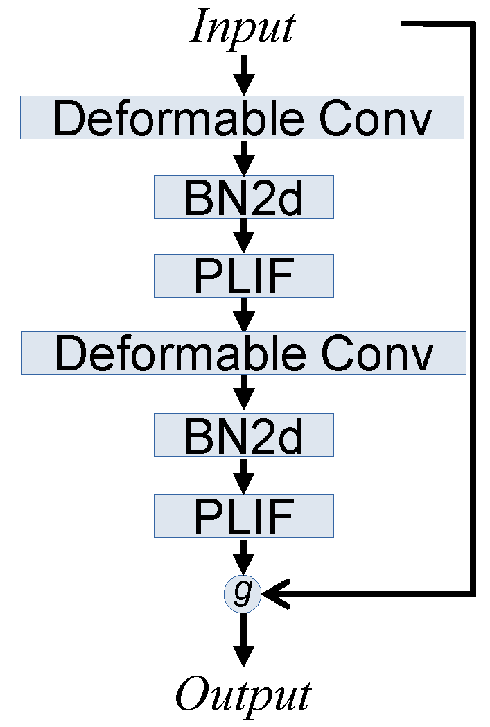
• We proposed a novel SNN-based model for HSI classification by integrating an attention mechanism and deformable convolution with a spiking ResNet. The spiking ResNet framework we used, named SEW ResNet, could overcome the vanishing/exploding gradient problems effectively. In addition, the temporal-channel joint attention (TCJA) mechanism was introduced for better feature extraction, by guiding the model to figure out what is useful and when, through filtering the abundant temporal and spectral information.
• For boundary-awareness, we proposed the deformable SEW ResNet method by adding the deformable convolutional mechanism into the SEW ResNet block. The deformable convolution provides variable receptive fields for high-level features extraction and brings our method the boundary-awareness to mitigate the boundary confusion phenomenon.

The rest of this article is organized as follows. Section 2 introduces the proposed methods used to build an attention-based deformable SNN model and the model architecture in detail. Section 3 presents the results of experiments. Section 4 summarizes this paper.

2. Proposed Method

Represent the original HSI cube as $\mathbf{X}={[x_1,x_2,x_3\dots x_B]}^{\mathrm{T}}\in {\mathcal{R}}^{(N\times M)\times B}$ with B spectral channels and $(N\times M)$ samples. All the pixels $x_i={[x_{i,1},x_{i,2},x_{i,3},\dots x_{i,B}]}^{\mathrm{T}}\in \mathbf{X}$ belong to $\mathbf{Y}=y_1,y_2,y_3,\dots y_c$ representing C land-cover classes. The proposed model’s framework for HSI classification comprises the spiking encoder, the spike-element-wise ResNet, the temporal-channel joint attention layer, the deformable spike-element-wise ResNet, the max-pooling layer, and the output layer. Figure 1 shows the framework of the proposed network, in which the methods we use will be introduced in detail in the following subsections.

Figure 1. Framework of the proposed SNN-based model for HSI classification. SEW block denotes the spiking element wise ResNet block as shown in Figure 4b; TCJA Layer denotes the temporal channel joint attention layer as shown in Figure 5; Deformable block denotes the deformable spiking element wise ResNet block as shown in Figures 8 and 9.

2.1. Leaky Integrate and Fire Model

As the fundamental computing unit of an SNN, spike neuron models play the role that activation functions play in the traditional ANNs. Furthermore, it is one of the main differences between SNNs and ANNs. The distinction between different spike neuron models lies in the extent of modeling of the biological neurons in the human brain. In terms of complexity, the current mainstream spike neuron models are divided into the Hodgkin–Huxley (HH) model [30], the lzhikevich model [31], the Leaky Integrate and Fire (LIF) model [32], and the Integrate and Fire (IF) model [33]. The HH model has the highest biological precision with enormous computation, and the IF model is quite the opposite. Considering the balance between computing cost and biological plausibility, we choose the LIF model as our spike neuron model. The neuron is modeled as a parallel Resistor-Capacitor (RC) [34] circuit as shown in Figure 2. $I\left(t\right)$ is the input current for the postsynaptic neuron at time t, which is parametrically related to the spikes emitted by the presynaptic neurons. There are two directions for the input current $I\left(t\right)$ after being inputted; one is to capacitor C for charging and integration, and another is to the resistor R for leakage, expressed as

$$I\left(t\right)=\frac{V\left(t\right)-V_{rest}}{R}+C\frac{\mathrm{d}V\left(t\right)}{\mathrm{d}t},$$

(1)

where $V\left(t\right)$ is the membrane potential at time t, $V_{rest}$ is the resting potential. Multiplying (1) by R and using $\tau =RC$ to represent the membrane time constant, we obtain the formula of subthreshold dynamics of the LIF model:

$$\tau \frac{\mathrm{d}V\left(t\right)}{\mathrm{d}t}=-(V\left(t\right)-V_{rest})+RI\left(t\right).$$

(2)

Figure 2. RC circuit of LIF model.

When the membrane potential $V\left(t\right)$ exceeds a preset threshold $V_{th}$, the neuron will emit a spike immediately to the postsynaptic neuron as one of its presynaptic neurons, and then $V\left(t\right)$ is reset to reset value $V_{reset}<V_{th}$. Meanwhile, the membrane potential constantly leaks according to $\tau$ until it reaches the rest value $V_{rest}$.

To enhance the characterization capabilities of the LIF model, we use a unified model named the parametric leaky integrate and fire (PLIF) model, based on [35]. This model contains a learnable membrane time constant, which makes the SNNs based on the PLIF model more robust than SNNs made on the LIF model.

2.2. Spiking Encoder

HSI is a stable image, which means there is no temporal information in it and the carrier of its data representation is the analog signal; it cannot be identified by SNNs directly. HSI should be coded into spike sequences by the spiking encoder first. To explain the information encoding mechanism, two broad categories of coding methods have been proposed—rate coding [36] and direct coding [37]. The analog value is converted to a spike sequence for rate coding using a Poisson generator function with a rate proportional to the input pixel value. The number of timesteps plays a significant role in the precision of rate coding. The larger the number of timesteps, the better the summation of the spike sequences from the encoder approximates the original pixel. Therefore, rate coding is limited by a lengthy processing period and slow information transmission. To explain the efficient and fast response mechanisms in our brains, we use direct coding, which has been widely adopted by many SNNs-based image classification works for our spiking encoder. Figure 3 shows the structure of the spiking encoder. First, we repeat the original HSI patch for T times. Then, the T patches were put into a learnable layer with spike neurons to generate the spiking images.

Figure 3. Illustration of the structure of spiking encoder.

2.3. Spiking Element-Wise Residual Network

After being converted to spatiotemporal spikes, the spiking HSI cube will be inputted into the feature extractor. To enhance the efficiency of the extractor by deepening the network, we use a spike-element-wise ResNet based on [24] as the fundamental structure for our extractor. The detail of the SEW block and the differences between it and the standard ResNet block are shown in Figure 4. Unlike previous spiking ResNets, [24] changes the activation function of the standard ResNet block proposed in [38], but also adjusts the position of the residual connection and uses an element-wise function g to substitute the original summation function. Specifically, [24] provides three different element-wise functions g, $ADD$, $AND$ and $IAND$, their expression is shown in Table 1. SEW ResNet can easily implement identity mapping and overcome the vanishing/exploding gradient problems, making the deeper SNNs achieve higher accuracy.

Figure 4. Illustration of (a) ResNet block and (b) Spike-element-wise block.

Table 1. Expression for element-wise functions.

Element-Wise Functions	Expression of $\mathit{g}(\mathit{a},\mathit{b})$
$ADD$	$a+b$
$AND$	$a\wedge b=a·b$
$IAND$	$(\neg a)\wedge b=(1-a)·b$

2.4. Temporal-Channel Joint Attention Mechanism

To further enhance the robustness of the proposed model, we introduce a kind of attention mechanism named temporal-channel joint attention based on [25] into our features extractor. The TCJA layer can effectively enforce the relevance of the spike sequence along both spatial and temporal dimensions. The detail of the mechanism is shown in Figure 5. The TCJA layer takes patched spiking HSI cube $\mathbf{P}\in {\mathcal{R}}^{(S\times S)\times B\times T}$ as input. Firstly, $\mathbf{P}$ is expressed in the dimension of spatial through the pooling layer to get the feature vector $\mathbf{U}\in {\mathcal{R}}^{(1\times 1)\times B\times T}$ defined as

$$\mathbf{U}={\mathcal{F}}_{exp}\left(\mathbf{P}\right)=\frac{1}{S\times S}\sum _{i=1}^S\sum _{j=1}^S\mathbf{P}(i,j).$$

(3)

Figure 5. Architecture of temporal-channel joint attention layer.

Two kinds of 1-D CNN are used to extract and learn the temporal and channel information of $\mathbf{U}$, respectively, of which the kernel sizes are a kind of hyper parameter. The output feature maps ${\mathbf{U}}_1$ and ${\mathbf{U}}_2$ are defined as

$$\begin{array}{cc}\hfill {\mathbf{U}}_1& ={\mathcal{F}}_{tem}\left(\mathbf{U}\right)=\mathbf{U}\ast w_{(1\times 1\times 3)}+b\hfill \\ \hfill {\mathbf{U}}_2& ={\mathcal{F}}_{cha}\left(\mathbf{U}\right)=\mathbf{U}\ast w_{(1\times 1\times 9)}+b,\hfill \end{array}$$

(4)

where ∗ denotes the 1-D convolution, and w and b are weights and bias of the 1-D convolutions. After that, we fuse the two feature vectors generated by the two 1-D CNN extractors to be the attention vector $\mathbf{V}\in {\mathcal{R}}^{(1\times 1)\times B\times T}$ defined as

$$\mathbf{V}={\mathcal{F}}_{fus}({\mathbf{U}}_1,{\mathbf{U}}_2)=\sigma ({\mathbf{U}}_1\odot {\mathbf{U}}_2),$$

(5)

where $\sigma$ denotes the sigmoid activation function and ⊙ is the element wise multiply operation. According to $\mathbf{V}$, we could select the features of the original spiking HSI cube $\mathbf{P}$ and get the output $\mathbf{Q}$, which contains more characterization.

2.5. Spiking Deformable Convolution Neural Networks

In order to utilize the spatial features, we select a patched image cube as one sample in which only the center pixel certainly carries the correct label. The other pixels around the center, especially the ones with different classes, may disturb the judgment of the classifier. As shown in Figure 6 (the classification map on Indian Pines of the SEWResNet [24]), the pixels on the boundary of a contiguous region with different classes are more likely to get wrong labels, called the salt-and-pepper phenomenon. We add a spiking deformable CNN [39] to the features extractor scheme to eliminate this phenomenon. As shown in Figure 7, deformable CNN could transform the shape of its receptive field to avoid the pixels with different class labels from the target pixel.

Figure 6. The classification map on Indian Pines of SEWResNet.

Figure 7. Illustration of the difference between the convolution kernel of regular CNN and deformable CNN.

The receptive field of the regular convolution is denoted as an immutable grid over the input x. For example, a $3\times 3$ kernel with dilation 1 is expressed as

$$D=\left\{\right(-1,-1),(-1,0),...,(0,1),(1,1\left)\right\}.$$

(6)

The output y is accumulated from each location $p_0$ and the locations around it within the range of grid D according to the weight w, expressed as

$$y\left(p_0\right)=\sum _{p_n\in D}w\left(p_n\right)·x(p_0+p_n),$$

(7)

where $p_n$ enumerates the locations in D.

In deformable convolution, a step named offset $\{△p_{n}n=1,...,N,N=D\}$ field generation is added before calculating the output feature map. The output y of deformable convolution is expressed as

$$y\left(p_0\right)=\sum _{p_n\in D}w\left(p_n\right)·x(p_0+p_n+△p_n).$$

(8)

As shown in Figure 8, the offsets are generated by convolutions over the input x. Due to the characteristics of convolutional calculation, the offset $△p_n$ is typically fractional. To determine a rational value, a bilinear interpolation kernel function F is used to implement the $x\left(p\right)$ as

$$x\left(p\right)=\sum _{q}F(q,p)·x\left(q\right),$$

(9)

where $p(p=p_0+p_n+△p_n)$ is the fractional location, q denotes all integral locations selected from input x, and F is expressed as

$$F(q,p)=f(q_x,p_x)·f(q_y,p_y),$$

(10)

where $f(a,b)=max(0,1-a-b)$.

Figure 8. Illustration of deformable convolution.

Furthermore, to avoid additional gradient problems, we proposed a deformable spike-element-wise block for the introduction of deformable CNN. Specifically, the deformable convolution models are plugged into the SEW Block to substitute the original CNN model. The detail of the deformable SEW Block is shown in Figure 9.

Figure 9. Illustration of deformable spike-element-wise block.

3. Experimental Results

In this section, we choose four CNN-based methods (ResNet [38], DPyResNet [18], SSRN [19], and A2S2KResNet [20]) one deformable-CNN-based model (DHCNet [29]), and one SNN-based model (HSI-SNN [28]) for comparison. To fully prove the effectiveness of the proposed method, the experiment was performed on five benchmark data sets: Indian Pines(IP), Kennedy Space Center (KSC), Houston University (HU), Pavia University (PU), and Salinas (SV). All experiments are conducted under the experimental environment of Ubuntu16, Titan-RTX GPUs, and 125G memory. We train and test the proposed model with the SpikingJelly [40] framework based on PyTorch [41]. Overall accuracy (OA), average accuracy (AA), and statistical kappa ($\kappa$) coefficient are used to evaluate the performance of the models.

3.1. Data Sets

AVIRIS [42] obtained the Indian Pines data set imaging of Indiana Indian Pine trees in the United States. Its spectrum is 200 (excluding 20 bands that cannot be reflected by water). Its size is $145\times 45$, composed of 21,025 pixels. There are 10,776 background pixels, and 10,249 object pixels used for training and testing are available.

Rosis-03 obtained the Pavia University data set [43] on Pavia City in Italy. It contains 103 available bands (12 noise affected by noise). Its size is $610\times 340$, including 207,400 pixels, of which 42,776 are object pixels.

The Salinas data set was shot by AVIRIS [42] sensors in Salinas Valley, California. The spatial resolution of these data is 3.7 m, and the size is $512\times 217$. The original data are 224 bands; after removing the bands with severe water vapor absorption, there are 204 bands left. These data include 16 crop categories.

The Houston University data set was obtained from the imaging of Houston University through the ITRES Casi-1500 sensor provided by the 2013 IEEE GRSS Data Fusion Contest. It has 144 bands. Its size is $349\times 1905$, of which 15,029 are object pixels.

The KSC data set was taken by AVIRIS [42] sensors at the Kennedy Space Center in Florida on 23 March 1996. These data contain 224 bands, leaving 176 bands after water vapor noise removal, with a spatial resolution of 18 m and a total of 13 categories.

Table 2 shows the main characteristics of the five data sets and the detail of our sample split strategy. Considering that the total sample size is close to or below 10,000, for IN and KSC data sets, we randomly select $10\%$ samples for training and $90\%$ for testing. While the extremely limited $1\%$ samples are randomly selected to train and $99\%$ to test for the other three data sets (PU, SV, and HU), their total sample sizes are big enough.

Table 2. The summary of IP, PU, SV, HU, and KSC data sets.

Characteristics	Data Sets
	IP	PU	SV	HU	KSC
Sensor	AVIRIS	ROSIS	AVIRIS	ITRES	AVIRIS
Spectral Bands	200	103	204	144	176
Spatial Size	$145\times 145$	$610\times 340$	$512\times 217$	$349\times 1905$	$512\times 614$
Classes	16	10	16	15	13
Total Samples	10,249	42,776	54,129	15,029	4211
Train Samples	1024	427	541	150	421
Test Samples	9225	42,349	53,588	14,879	3790

3.2. Experimental Setup and Parameter Evaluation

We train the proposed model using the stochastic gradient descent (SGD) optimizer and choose the cross entropy loss function to represent loss. The batch size is set to 32, and the learning rate is set to 0.1. The hyperparameters initial $\tau$ of PLIF, the kernel size of channel attention 1D-CNN $k_c$, and temporal attention 1D-CNN $k_t$ for the TCJA layer are uniformly set to 2.0, 9, and 3, respectively. The experiment is repeated five times, using 200 epochs each time. The model with the highest accuracy in the validation process is selected for evaluation on test samples.

Firstly, the experiment on the KSC data set is implemented for the evaluation of element-wise functions g in SEW ResNet. Table 3 shows the accuracy of the proposed model using different element-wise functions. It is observed that model with the $IAND$ function gets optimal results, while the other two functions are more likely to fall into the vanishing/exploding gradient problems. Thus, we set the element-wise function g to $IAND$ for the following experiments.

Table 3. Classification accuracy for different element-wise functions on the KSC data set.

g	OA (%)	AA (%)	$\mathit{\kappa }$
$ADD$	97.65 ± 0.007	95.66 ± 0.013	0.9738 ± 0.008
$AND$	82.91 ± 0.121	75.91 ± 0.137	0.8075 ± 0.137
$IAND$	99.13 ± 0.002	96.13 ± 0.020	0.9901 ± 0.003

The patch size of the input samples is an essential parameter for the extraction of spatial information, and it also influences the extension of disturbance from pixels with different classes. A smaller patch size will limit the model’s spatial feature extraction, decreasing classification accuracy. In contrast, a bigger patch size will aggravate the salt-and-pepper phenomenon. During these experiments, the timestep is set to 8. Table 4 shows the classification accuracy of the five data sets with four different patch sizes ($7\times 7$, $9\times 9$, $11\times 11$, and $13\times 13$). The five data sets’ best results are achieved using patch size $11\times 11$ and $13\times 13$. Noting that a bigger patch size will make the other models achieve worse results, we fix $11\times 11$ as the patch size of the proposed method for all the data sets for fair comparisons.

Table 4. Classification accuracy for different patch sizes on the five data sets.

Data Set	Patch Size	OA (%)	AA (%)	$\mathit{\kappa }$
IP	$7\times 7$	98.71 ± 0.002	95.37 ± 0.021	0.9852 ± 0.002
	$9\times 9$	99.05 ± 0.002	95.24 ± 0.011	0.9891 ± 0.002
	$11\times 11$	99.15 ± 0.003	95.30 ± 0.018	0.9904 ± 0.003
	$13\times 13$	99.13 ± 0.002	96.13 ± 0.020	0.9901 ± 0.003
PU	$7\times 7$	95.41 ± 0.005	93.41 ± 0.008	0.9389 ± 0.007
	$9\times 9$	95.89 ± 0.006	93.51 ± 0.012	0.9453 ± 0.009
	$11\times 11$	96.55 ± 0.005	93.58 ± 0.019	0.9542 ± 0.007
	$13\times 13$	96.58 ± 0.004	93.16 ± 0.019	0.9545 ± 0.006
SV	$7\times 7$	97.37 ± 0.002	98.71 ± 0.002	0.9707 ± 0.003
	$9\times 9$	98.51 ± 0.003	99.16 ± 0.002	0.9834 ± 0.003
	$11\times 11$	99.00 ± 0.003	99.27 ± 0.001	0.9888 ± 0.003
	$13\times 13$	99.14 ± 0.002	98.93 ± 0.005	0.9905 ± 0.003
HU	$7\times 7$	83.59 ± 0.016	84.31 ± 0.013	0.8224 ± 0.017
	$9\times 9$	85.65 ± 0.013	86.28 ± 0.011	0.8448 ± 0.014
	$11\times 11$	85.78 ± 0.008	86.07 ± 0.006	0.8462 ± 0.008
	$13\times 13$	85.86 ± 0.012	86.02 ± 0.011	0.8471 ± 0.013
KSC	$7\times 7$	99.01 ± 0.012	97.81 ± 0.033	0.9890 ± 0.013
	$9\times 9$	99.30 ± 0.005	98.83 ± 0.009	0.9922 ± 0.006
	$11\times 11$	99.53 ± 0.002	99.15 ± 0.004	0.9947 ± 0.002
	$13\times 13$	99.52 ± 0.003	99.11 ± 0.006	0.9946 ± 0.004

The timestep is another critical parameter for an SNN-based model. A tinier timestep limits the model’s ability to extract features of HSIs, and a longer timestep will enhance computational energy consumption. Table 5 shows the evaluation results for different timesteps (4, 8, 12, 16) on five data sets. The best OA, AA, and $\kappa$ are achieved using timesteps 12 and 16. Considering the computational consumption, we set 12 as the timestep for the proposed model.

Table 5. Classification accuracy for different timesteps on the five data sets.

Data Set	Timestep	OA (%)	AA (%)	$\mathit{\kappa }$
IP	4	99.22 ± 0.002	96.33 ± 0.015	0.9912 ± 0.003
	8	99.16 ± 0.003	95.30 ± 0.018	0.9904 ± 0.003
	12	99.16 ± 0.003	95.84 ± 0.011	0.9905 ± 0.003
	16	99.18 ± 0.003	96.36 ± 0.015	0.9907 ± 0.003
PU	4	95.24 ± 0.009	90.72 ± 0.032	0.9366 ± 0.012
	8	96.55 ± 0.005	93.58 ± 0.019	0.9542 ± 0.007
	12	96.51 ± 0.006	93.96 ± 0.015	0.9537 ± 0.008
	16	96.79 ± 0.004	94.22 ± 0.008	0.9574 ± 0.006
SV	4	99.00 ± 0.002	99.36 ± 0.001	0.9888 ± 0.002
	8	99.00 ± 0.003	99.27 ± 0.001	0.9888 ± 0.003
	12	99.03 ± 0.002	99.28 ± 0.001	0.9892 ± 0.002
	16	99.10 ± 0.002	99.16 ± 0.002	0.9900 ± 0.002
HU	4	85.59 ± 0.015	85.80 ± 0.014	0.8441 ± 0.016
	8	85.78 ± 0.008	86.07 ± 0.006	0.8462 ± 0.008
	12	86.29 ± 0.017	86.63 ± 0.014	0.8517 ± 0.018
	16	86.03 ± 0.014	86.63 ± 0.012	0.8489 ± 0.016
KSC	4	99.54 ± 0.001	99.15 ± 0.003	0.9949 ± 0.001
	8	99.53 ± 0.002	99.15 ± 0.004	0.9947 ± 0.002
	12	99.53 ± 0.003	99.22 ± 0.004	0.9948 ± 0.003
	16	99.60 ± 0.003	99.25 ± 0.008	0.9956 ± 0.004

3.3. Classification Results

Table 6, Table 7 and Table 8 show the average OAs, AAs, κs, and accuracies for every class of the five repeat processes on four data sets (IP, PU, SV, and HU). Moreover, our proposed method obtains competitive results in all data sets, compared with the other ResNet-based, deformable-CNN-based, and SNN-based methods.

Table 6. Classification accuracy obtained by different methods for the Indian Pines data set.

Classes	ResNet	DpyResNet	SSRN	A2S2KResNet	DHCNet	HSI-SNN	BDSNN
1	97.01 ± 0.039	99.29 ± 0.014	78.12 ± 0.392	98.99 ± 0.012	92.49 ± 0.122	37.62 ± 17.651	85.65 ± 0.045
2	91.54 ± 0.039	91.00 ± 0.025	98.42 ± 0.006	98.65 ± 0.003	97.91 ± 0.017	93.20 ± 2.047	99.28 ± 0.005
3	89.17 ± 0.075	88.62 ± 0.045	97.03 ± 0.010	97.78 ± 0.009	98.41 ± 0.011	93.36 ± 1.532	99.18 ± 0.006
4	96.39 ± 0.043	97.60 ± 0.041	98.11 ± 0.021	95.05 ± 0.075	95.17 ± 0.046	92.99 ± 6.150	99.26 ± 0.007
5	96.82 ± 0.030	95.07 ± 0.050	96.39 ± 0.012	98.30 ± 0.030	96.57 ± 0.030	94.02 ± 1.199	98.86 ± 0.021
6	96.94 ± 0.023	96.15 ± 0.016	98.14 ± 0.010	99.15 ± 0.011	97.83 ± 0.015	97.38 ± 1.865	99.01 ± 0.007
7	84.88 ± 0.222	93.60 ± 0.128	57.89 ± 0.474	92.64 ± 0.106	65.39 ± 0.135	39.23 ± 19.521	88.57 ± 0.206
8	96.87 ± 0.027	96.68 ± 0.017	99.18 ± 0.015	100.0 ± 0.000	99.69 ± 0.003	99.58 ± 0.612	100.0 ± 0.000
9	50.29 ± 0.421	59.78 ± 0.350	60.00 ± 0.490	80.71 ± 0.215	57.06 ± 0.211	75.56 ± 13.426	76.12 ± 0.181
10	94.53 ± 0.025	93.60 ± 0.025	97.73 ± 0.006	98.57 ± 0.012	98.14 ± 0.011	92.00 ± 3.324	98.83 ± 0.008
11	93.16 ± 0.027	94.23 ± 0.025	99.31 ± 0.004	99.35 ± 0.002	98.49 ± 0.003	96.87 ± 0.835	99.55 ± 0.001
12	92.81 ± 0.036	89.68 ± 0.039	96.37 ± 0.024	97.67 ± 0.002	92.18 ± 0.051	91.09 ± 2.713	98.85 ± 0.015
13	96.16 ± 0.029	93.38 ± 0.063	99.00 ± 0.005	99.13 ± 0.011	97.97 ± 0.025	95.35 ± 3.692	99.63 ± 0.008
14	97.32 ± 0.027	95.27 ± 0.052	99.30 ± 0.004	99.96 ± 0.000	98.89 ± 0.006	97.72 ± 0.937	99.96 ± 0.000
15	91.40 ± 0.076	95.85 ± 0.038	98.86 ± 0.009	99.56 ± 0.006	96.26 ± 0.016	93.39 ± 4.529	99.81 ± 0.003
16	94.85 ± 0.031	93.39 ± 0.046	86.60 ± 0.129	96.76 ± 0.041	84.06 ± 0.191	85.48 ± 8.532	90.92 ± 0.067
OA(%)	93.59 ± 0.006	93.30 ± 0.013	98.22 ± 0.003	98.82 ± 0.003	97.18 ± 0.010	94.58 ± 0.425	99.16 ± 0.003
AA(%)	91.26 ± 0.020	92.07 ± 0.019	91.28 ± 0.072	97.02 ± 0.017	91.66 ± 0.037	85.93 ± 1.595	95.84 ± 0.011
$\kappa \times 100$	92.68 ± 0.007	92.34 ± 0.015	97.98 ± 0.003	98.66 ± 0.003	96.79 ± 0.011	93.83 ± 0.483	99.05 ± 0.003

Table 7. Classification accuracy obtained by different methods for the Pavia University data set.

Classes	ResNet	DpyResNet	SSRN	A2S2KResNet	DHCNet	HSI-SNN	BDSNN
1	67.90 ± 0.046	64.40 ± 0.045	84.48 ± 0.115	91.01 ± 0.061	82.50 ± 0.072	94.14 ± 4.848	96.76 ± 0.011
2	86.93 ± 0.033	85.87 ± 0.062	97.45 ± 0.009	99.65 ± 0.004	93.29 ± 0.028	99.43 ± 0.194	99.95 ± 0.001
3	72.96 ± 0.192	70.01 ± 0.076	78.35 ± 0.091	83.68 ± 0.090	71.33 ± 0.179	70.09 ± 25.499	87.03 ± 0.015
4	98.32 ± 0.025	98.03 ± 0.016	98.16 ± 0.015	88.01 ± 0.058	96.55 ± 0.026	85.92 ± 3.552	94.64 ± 0.018
5	96.97 ± 0.014	99.06 ± 0.012	99.76 ± 0.003	99.73 ± 0.002	98.52 ± 0.013	79.28 ± 31.758	99.51 ± 0.003
6	90.36 ± 0.098	95.74 ± 0.020	94.49 ± 0.028	89.49 ± 0.019	89.08 ± 0.149	97.42 ± 1.977	97.70 ± 0.024
7	89.46 ± 0.086	82.18 ± 0.095	85.19 ± 0.110	77.49 ± 0.129	81.49 ± 0.139	65.18 ± 34.707	98.65 ± 0.011
8	75.17 ± 0.074	73.64 ± 0.118	74.25 ± 0.073	70.62 ± 0.304	75.89 ± 0.089	88.02 ± 5.959	84.65 ± 0.031
9	89.87 ± 0.091	95.51 ± 0.037	85.87 ± 0.188	90.41 ± 0.039	79.11 ± 0.092	53.67 ± 16.771	86.74 ± 0.108
OA(%)	82.29 ± 0.015	80.93 ± 0.031	90.87 ± 0.028	92.11 ± 0.036	87.05 ± 0.030	92.27 ± 3.011	96.51 ± 0.006
AA(%)	85.33 ± 0.029	84.94 ± 0.021	88.67 ± 0.033	87.79 ± 0.036	85.31 ± 0.024	81.46 ± 9.872	93.96 ± 0.015
$\kappa \times 100$	75.65 ± 0.022	73.54 ± 0.049	87.85 ± 0.038	89.48 ± 0.048	82.54 ± 0.042	89.68 ± 4.065	95.37 ± 0.008

Table 8. Classification accuracy obtained by different methods for the houston13 data set.

Classes	ResNet	DpyResNet	SSRN	A2S2KResNet	DHCNet	HSI-SNN	BDSNN
1	73.06 ± 0.136	65.05 ± 0.065	86.57 ± 0.034	88.47 ± 0.036	85.82 ± 0.069	88.99 ± 1.902	96.26 ± 0.032
2	82.99 ± 0.194	84.57 ± 0.040	87.17 ± 0.083	89.89 ± 0.044	80.94 ± 0.111	84.57 ± 10.127	90.18 ± 0.032
3	99.82 ± 0.004	98.71 ± 0.016	97.95 ± 0.020	97.90 ± 0.015	98.36 ± 0.169	93.72 ± 2.236	98.01 ± 0.007
4	54.85 ± 0.254	76.71 ± 0.051	89.70 ± 0.050	82.35 ± 0.135	86.53 ± 0.110	82.58 ± 6.485	93.56 ± 0.047
5	90.54 ± 0.036	92.21 ± 0.030	95.30 ± 0.032	94.91 ± 0.063	92.01 ± 0.093	99.97 ± 0.040	100.0 ± 0.000
6	97.86 ± 0.019	95.01 ± 0.048	83.21 ± 0.209	85.64 ± 0.056	84.50 ± 0.114	44.60 ± 25.611	78.25 ± 0.043
7	45.28 ± 0.096	58.80 ± 0.064	68.64 ± 0.084	74.75 ± 0.101	62.67 ± 0.173	62.53 ± 6.847	84.11 ± 0.038
8	77.63 ± 0.234	83.99 ± 0.195	88.14 ± 0.020	64.38 ± 0.073	74.31 ± 0.214	50.70 ± 4.932	65.31 ± 0.026
9	31.12 ± 0.124	42.40 ± 0.091	74.69 ± 0.114	59.23 ± 0.149	55.99 ± 0.171	60.57 ± 8.536	70.98 ± 0.093
10	54.67 ± 0.172	35.89 ± 0.104	67.66 ± 0.040	75.08 ± 0.123	53.10 ± 0.136	78.37 ± 7.400	85.29 ± 0.083
11	34.63 ± 0.141	29.99 ± 0.067	72.86 ± 0.142	78.80 ± 0.086	52.89 ± 0.203	87.21 ± 7.149	84.67 ± 0.087
12	46.66 ± 0.168	55.95 ± 0.063	74.40 ± 0.104	71.28 ± 0.153	68.50 ± 0.076	71.37 ± 18.924	81.82 ± 0.066
13	45.52 ± 0.306	49.50 ± 0.212	82.63 ± 0.087	62.21 ± 0.244	42.15 ± 0.325	60.00 ± 13.145	71.59 ± 0.047
14	97.79 ± 0.018	98.02 ± 0.017	95.94 ± 0.020	98.86 ± 0.011	95.71 ± 0.049	96.32 ± 4.789	99.38 ± 0.047
15	95.73 ± 0.022	95.88 ± 0.025	95.50 ± 0.019	99.44 ± 0.010	91.10 ± 0.055	97.92 ± 2.089	100.0 ± 0.000
AA(%)	57.53 ± 0.062	60.23 ± 0.028	80.84 ± 0.017	80.07 ± 0.023	69.20 ± 0.029	77.73 ± 0.557	86.29 ± 0.017
OA(%)	68.54 ± 0.045	70.84 ± 0.012	84.02 ± 0.010	81.55 ± 0.025	74.97 ± 0.048	77.29 ± 0.843	86.63 ± 0.014
$\kappa \times 100$	54.00 ± 0.067	56.93 ± 0.030	79.29 ± 0.019	78.44 ± 0.025	66.65 ± 0.031	75.92 ± 0.595	85.17 ± 0.018

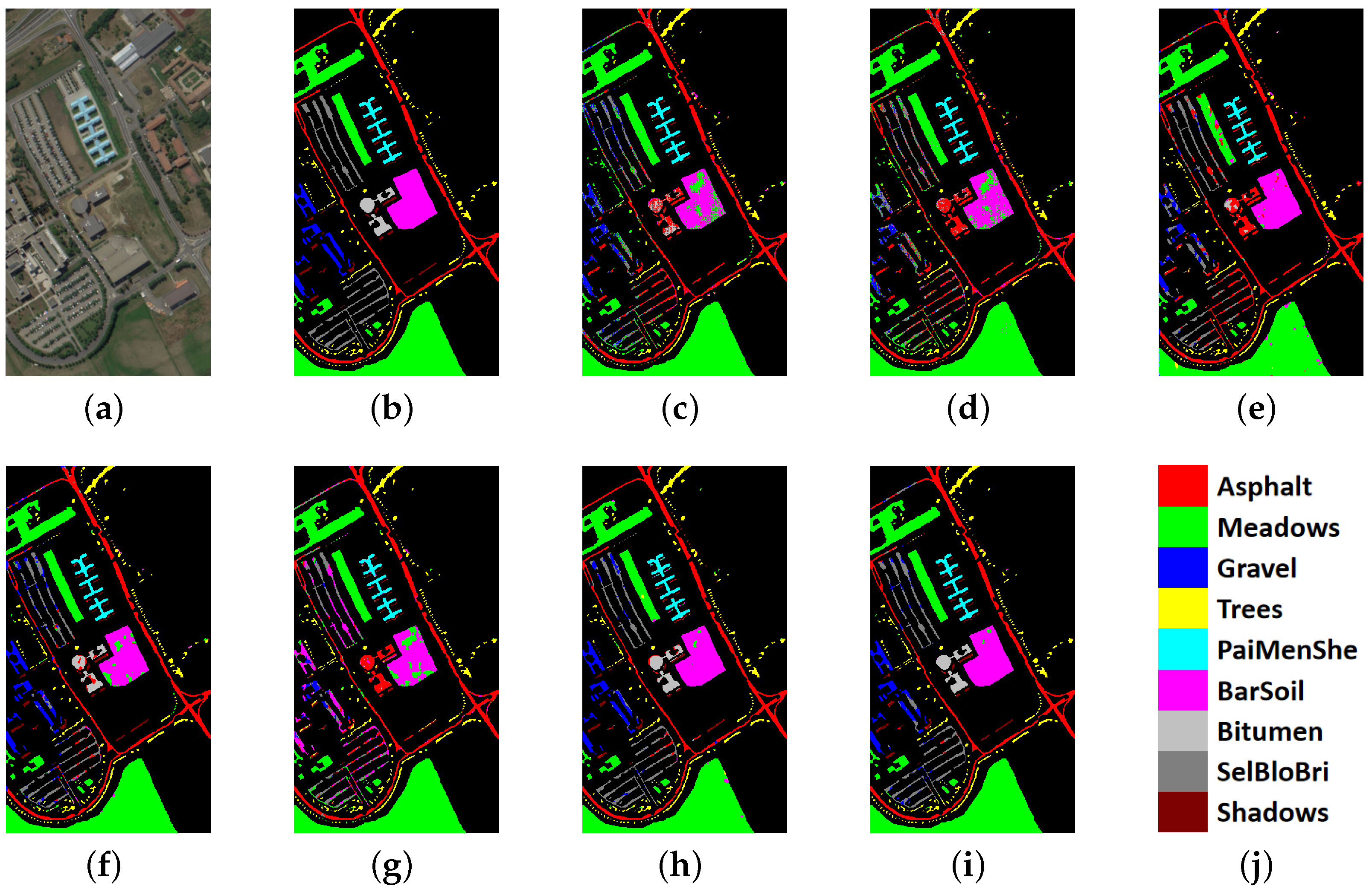
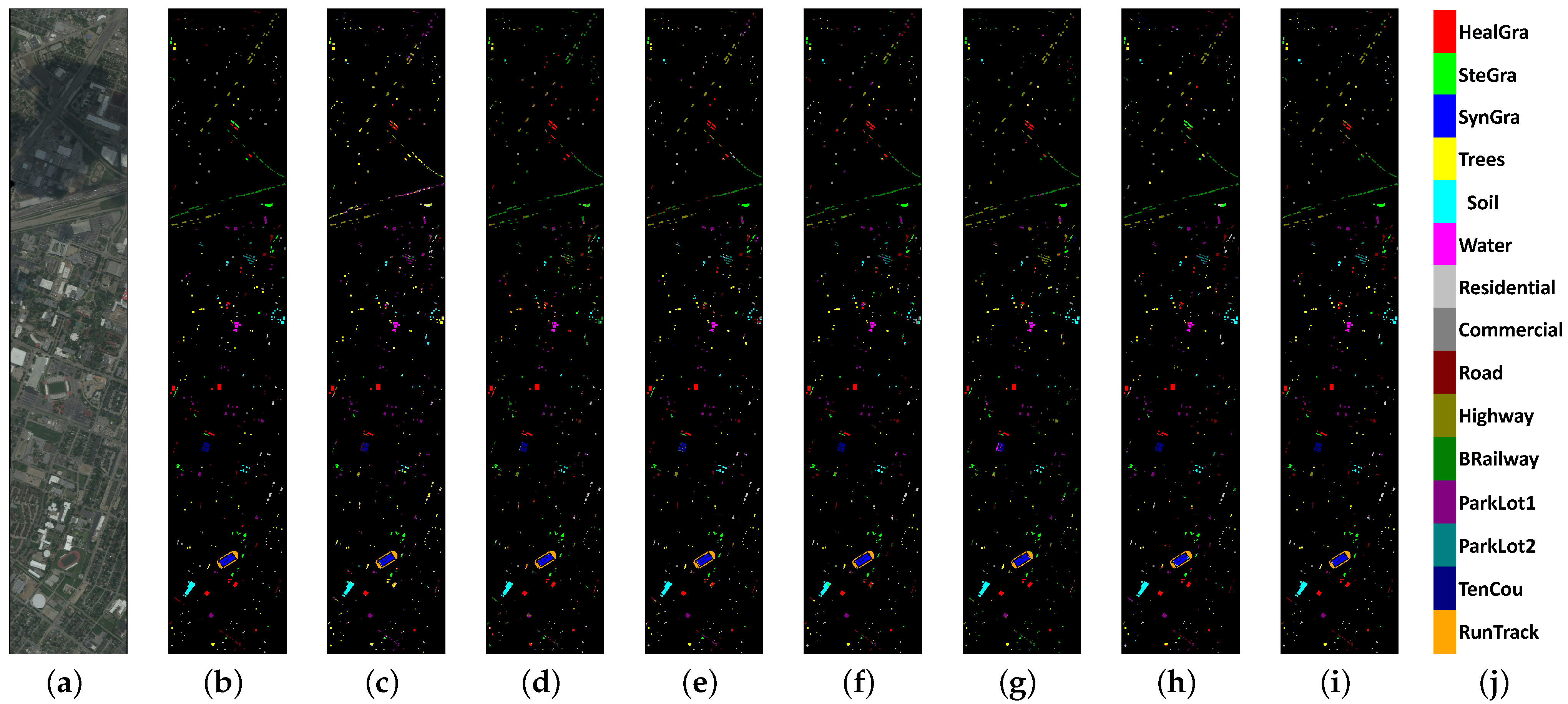
The results for the IP data set are shown in Table 6, and Figure 10 shows the classification maps of our model and others for comparison. Our model achieves the best OA (99.16 ± 0.003%), which is 0.34% higher than the best CNN-based model (A2S2KResNet) and 4.58% higher than HSI-SNN. In addition, the proposed model also achieves the biggest $\kappa$. However, the AA of the proposed model is 1.18% lower than A2S2KResNet, expressing the worse robustness of the SNN-based model for the IP data set, which has an uneven number of categories.

Figure 10. Classification results of the Indian Pines data set. (a) False-color composite image. (b) Ground truth. (c) ResNet. (d) DPyResNet. (e) SSRN. (f) A2S2KResNet. (g) DHCNet. (h) HSI-SNN. (i) Proposed BDSNN. (j) Color labels.

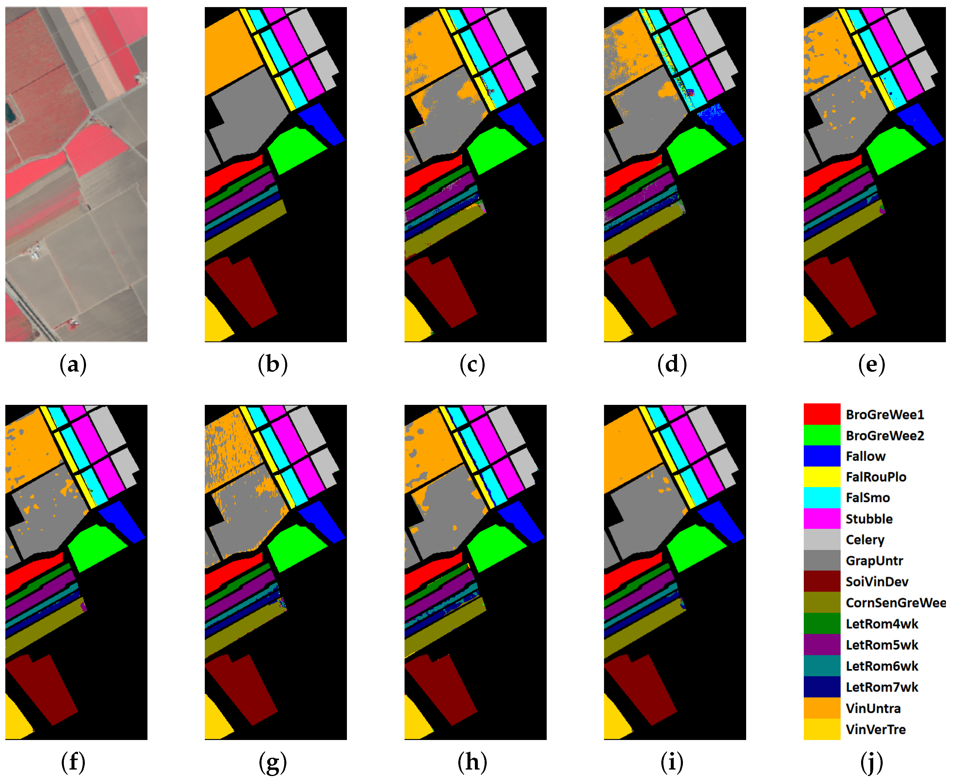
For the PU data set, the results are shown in Table 7. The proposed model achieves the best OA (96.15 ± 0.006%), which is 4.24% higher than the best results of the other models. And the proposed model also obtains a higher AA (93.96 ± 0.015%) and $\kappa$ (0.9537 ± 0.008) than the others. The classification maps are shown in Figure 11.

Figure 11. Classification results of the Pavia University data set. (a) False-color composite image. (b) Ground truth. (c) ResNet. (d) DPyResNet. (e) SSRN. (f) A2S2K. (g) DHCNet. (h) HSI-SNN. (i) Proposed BDSNN. (j) Color labels.

Table 9 shows the results for the SV data set. The proposed model achieves the best OA (99.03 ± 0.002%), which is 5.45% higher than the best results of the other models. And the proposed model also obtains a higher AA (99.28 ± 0.001%) and $\kappa$ (0.9892 ± 0.002) than the others. The classification maps are shown in Figure 12.

Table 9. Classification accuracy obtained by different methods for the Salinas data set.

Classes	ResNet	DpyResNet	SSRN	A2S2KResNet	DHCNet	HSI-SNN	BDSNN
1	99.12 ± 0.017	99.33 ± 0.006	99.86 ± 0.003	98.17 ± 0.036	99.95 ± 0.001	98.53 ± 2.294	99.40 ± 0.008
2	97.34 ± 0.048	98.57 ± 0.010	100.0 ± 0.000	100.0 ± 0.000	99.35 ± 0.012	99.96 ± 0.076	100.0 ± 0.000
3	97.72 ± 0.025	96.72 ± 0.023	97.47 ± 0.049	99.94 ± 0.001	99.48 ± 0.003	99.88 ± 0.083	100.0 ± 0.000
4	96.95 ± 0.023	95.92 ± 0.024	96.17 ± 0.027	99.88 ± 0.002	97.97 ± 0.015	96.25 ± 3.665	98.95 ± 0.017
5	93.39 ± 0.114	93.75 ± 0.082	99.11 ± 0.012	98.07 ± 0.009	99.15 ± 0.010	95.97 ± 5.669	99.41 ± 0.007
6	99.38 ± 0.006	99.57 ± 0.005	99.94 ± 0.001	100.0 ± 0.000	99.54 ± 0.004	99.64 ± 0.714	100.0 ± 0.000
7	99.61 ± 0.006	99.74 ± 0.003	99.97 ± 0.000	99.94 ± 0.001	99.86 ± 0.002	99.91 ± 0.077	99.99 ± 0.000
8	88.04 ± 0.046	88.39 ± 0.061	88.49 ± 0.050	95.57 ± 0.017	89.47 ± 0.045	92.93 ± 4.579	97.25 ± 0.008
9	98.76 ± 0.011	98.96 ± 0.008	99.94 ± 0.001	99.98 ± 0.000	99.77 ± 0.002	99.99 ± 0.013	100.0 ± 0.000
10	98.94 ± 0.011	97.74 ± 0.013	98.67 ± 0.013	98.33 ± 0.010	99.18 ± 0.007	96.60 ± 1.553	99.37 ± 0.010
11	97.22 ± 0.043	95.86 ± 0.071	97.95 ± 0.027	99.77 ± 0.004	99.55 ± 0.006	98.00 ± 1.572	99.83 ± 0.003
12	95.94 ± 0.051	89.02 ± 0.140	99.34 ± 0.012	98.79 ± 0.009	96.06 ± 0.053	99.38 ± 0.784	99.85 ± 0.002
13	86.31 ± 0.119	85.36 ± 0.097	92.80 ± 0.035	98.13 ± 0.009	85.77 ± 0.076	85.54 ± 1.361	99.51 ± 0.005
14	88.31 ± 0.150	91.78 ± 0.054	98.18 ± 0.003	98.07 ± 0.005	94.52 ± 0.043	93.40 ± 7.725	97.06 ± 0.016
15	80.85 ± 0.061	80.03 ± 0.051	92.04 ± 0.009	89.73 ± 0.028	82.17 ± 0.036	94.57 ± 3.371	98.62 ± 0.012
16	99.94 ± 0.001	99.69 ± 0.004	99.65 ± 0.007	99.30 ± 0.007	99.46 ± 0.009	98.10 ± 1.100	99.32 ± 0.010
OA(%)	92.69 ± 0.012	92.41 ± 0.011	95.79 ± 0.013	97.28 ± 0.003	94.49 ± 0.012	96.70 ± 1.364	99.03 ± 0.002
AA(%)	94.86 ± 0.015	94.40 ± 0.006	97.47 ± 0.006	98.35 ± 0.004	96.33 ± 0.010	96.79 ± 1.310	99.28 ± 0.001
$\kappa \times 100$	91.85 ± 0.013	91.55 ± 0.013	95.31 ± 0.014	96.97 ± 0.003	93.86 ± 0.014	96.33 ± 1.515	98.92 ± 0.002

Figure 12. Classification results of the Salinas data set. (a) False-color composite image. (b) Ground truth. (c) ResNet. (d) DPyResNet. (e)SSRN. (f)A2S2KResNet. (g) DHCNet. (h) HSI-SNN. (i) Proposed BDSNN. (j) Color labels.

Table 8 shows the results for the HU data set. The proposed model achieves the best OA (86.29 ± 0.017%), which is 4.24% higher than the best results of the other models. And the proposed model also obtains a higher AA (86.63 ± 0.014%) and $\kappa$ (0.8517 ± 0.018) than the others. The classification maps are shown in Figure 13.

Figure 13. Classification result of the Houston13 data set. (a) False-color composite image. (b) Ground truth. (c) ResNet. (d) DPyResNet. (e) SSRN. (f) A2S2K. (g) DHCNet. (h) HSI-SNN. (i) Proposed BDSNN. (j) Color labels.

3.4. Ablation Study

In order to further validate the methods we used in our proposed model, we evaluate the generalization performance for the HU data set of the proposed model and three other models without the specific methods we used. The details of the models are as follows:

• Denoted as SEW + TCJA, the deformable CNN is removed from the proposed framework.
• Denoted as SEW + DEF, the TCJA layer is removed from the proposed framework.
• Denoted as SEW, the deformable CNN and TCJA layers are both removed from the proposed framework.

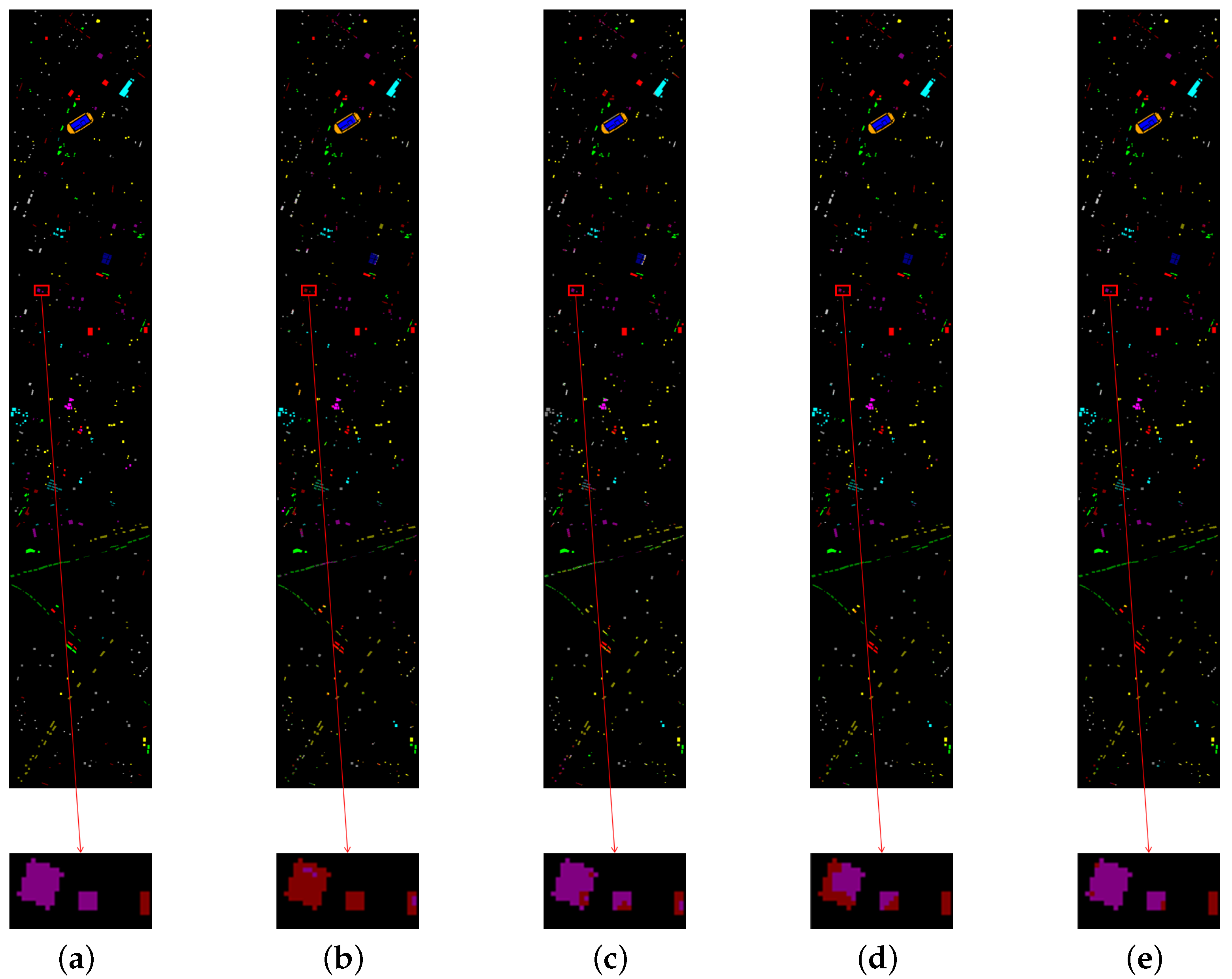
For the ablation experiments, we change the patch size to $13\times 13$ to better reflect the boundary effect and keep the other experimental settings unchanged. Table 10 shows the classification results of the ablation experiments over HU data sets. Compared with SEW, SEW + DEF, SEW + TCJA, and the proposed model produce notable improvement in all of the three matrices (OA, AA, and $\kappa$). Regarding OA, the TCJA layer method used in SEW + TCJA and the proposed model achieves 10.24% and 10.41% improvement than SEW and SEW + DEF, respectively. Furthermore, the deformable CNN method used in SEW + DEF and the proposed model obtain 0.63% and 0.8% advances compared with SEW and SEW + TCJA, respectively. 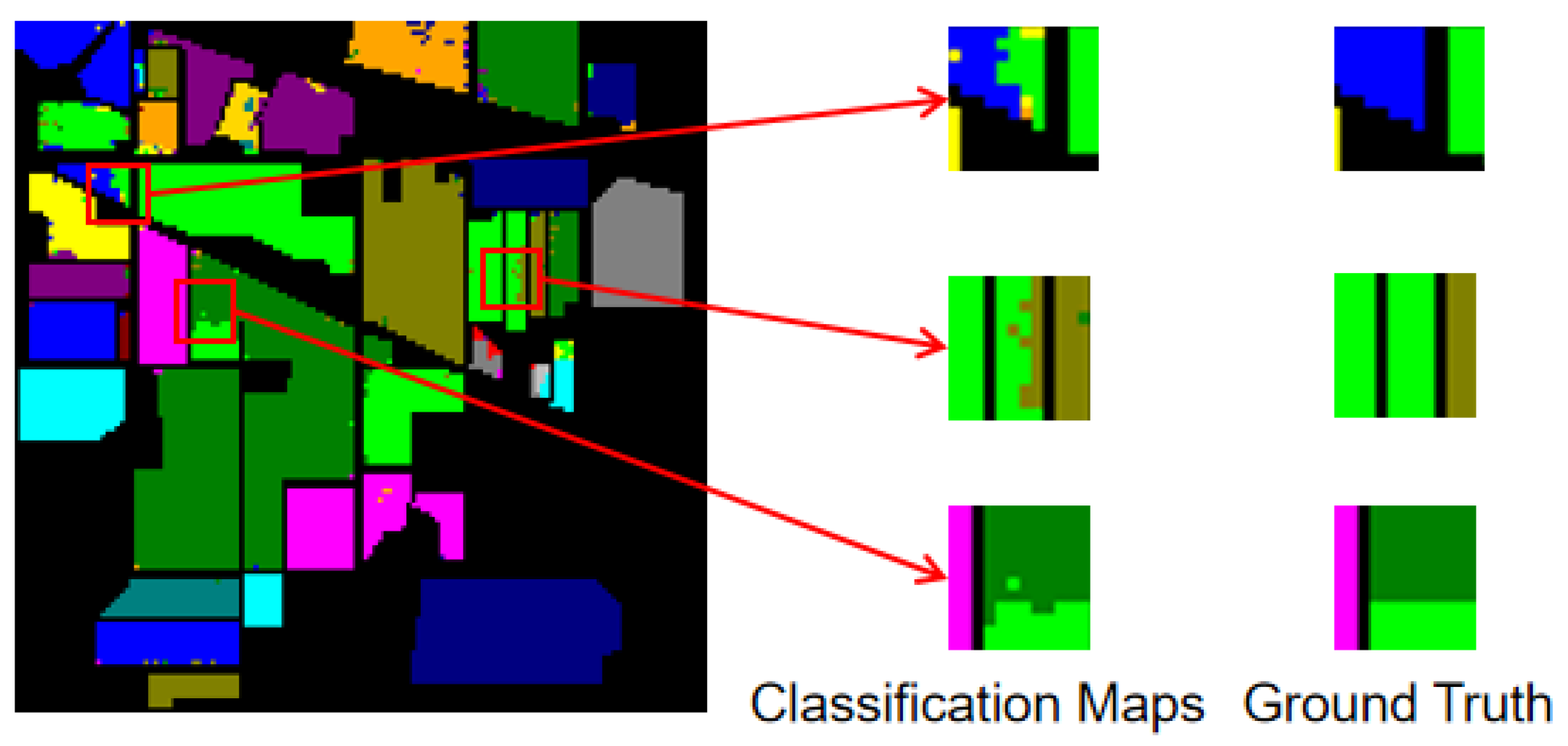The classification maps are shown in Figure 14. We can observe that the deformable CNN method can mitigate the boundary confusion phenomenon.

Table 10. The results of the ablation experiments.

Matrices	Models
	SEW	SEW + DEF	SEW + TCJA	Proposed
OA(%)	75.55 ± 0.017	76.18 ± 0.014	85.79 ± 0.014	86.59 ± 0.016
AA(%)	75.95 ± 0.015	76.74 ± 0.019	86.05 ± 0.014	86.79 ± 0.015
$\kappa \times 100$	73.54 ± 0.018	74.22 ± 0.015	84.63 ± 0.015	85.49 ± 0.018

Figure 14. Classification results of the ablation experiments. (a) Ground truth. (b) SEW. (c) SEW + DEF. (d) SEW + TCJA. (e) Proposed BDSNN.

3.5. Comparison of Running Times

In this section, the training and testing time of three representative CNN-based methods and our proposed BDSNN on four data sets are shown in Table 11. Due to the limitations of the computing platform, we can only estimate the time on nonneuromorphic computers. As a result, all of the traditional deep learning methods have an advantage in training and test time compared with our proposed BDSNN, while the advantages of SNN in terms of energy saving and faster computing can only be demonstrated with the application to neuromorphic computers [44]. Concerning the SNN-based HSI-SNN, the time and OA are shown in Table 12. The training time of our proposed BDSNN is about 1.82–3.24 times as long as the training time of HSI-SNN and about 3.61–7.73 times in terms of test time, with about a 2.33–8.56% improvement of OA. Due to a more complex structure, the proposed BDSNN has a disadvantage in running times. The introductions of TCJA and deformable convolution create a burden for computation, as they have many non-spiking calculation processes, such as attention vector generation and offset generation. The solution to reducing the implications for computational efficiency will be one of our future research directions.

Table 11. Training time and test time of DpyResNet, SSRN, A2S2KResNet, and BDSNN for the four data sets.

Methods	Time (s)	IP	PU	SV	HU
DpyResNet	Training	923.02	302.65	453.48	298.28
	Test	59.20	256.47	360.98	202.12
SSRN	Training	1401.74	206.94	1056.48	98.63
	Test	20.60	58.24	134.52	30.68
A2S2KResNet	Training	1682.08	576.26	1055.07	301.42
	Test	26.23	151.84	238.55	94.64
BDSNN	Training	2352.68	955.68	1126.49	340.63
	Test	83.14	432.55	537.22	146.97

Table 12. Training time, test time, and OA of HSI-SNN and BDSNN for the four data sets.

Methods	Time (s) & OA(%)	IP	PU	SV	HU
HSI-SNN	Training	1155.07	415.47	618.7	105.23
	Test	23.04	103.26	72.66	19.01
	OA	94.58	92.27	96.70	77.73
BDSNN	Training	2352.68	955.68	1126.49	340.63
	Test	83.14	432.55	537.22	146.97
	OA	99.16	96.51	99.03	86.29

4. Conclusions

In this article, we proposed a boundary-aware deformable spiking neural network (BDSNN) for HSI classification. The proposed SNN is made of PLIF neurons, and the method for the spiking coder belongs to a direct coding scheme. The spiking element-wise ResNet is used for the proposed model to overcome the vanishing/exploding gradient problems. Moreover, the temporal-channel joint attention layer is introduced for effective temporal-spectral feature extraction. Furthermore, to mitigate boundary confusion, we introduced deformable CNN into SNN for the first time. By performing experiments on four hyperspectral data sets, it is proved that the proposed model outperforms other CNN-based models and an SNN-based model with limited training samples. The proposed BDSNN provides a promising way to improve the SNN-based methods for HSI classification. However, the running times comparison experiments show the limitations of BDSNN. While improving the feature extraction ability, the complex structure of BDSNN also increases the computational overhead. Therefore, we will pay attention to converting the non-spiking calculation processes into a spiking version of them in the future.

References

- Teke, M.; Deveci, H.S.; Haliloğlu, O.; Gürbüz, S.Z.; Sakarya, U. A short survey of hyperspectral remote sensing applications in agriculture. In Proceedings of the 2013 6th International Conference on Recent Advances in Space Technologies (RAST), IEEE, Istanbul, Turkey, 12–14 June 2013; pp. 171–176. [Google Scholar]
- Resmini, R.; Kappus, M.; Aldrich, W.; Harsanyi, J.; Anderson, M. Mineral mapping with hyperspectral digital imagery collection experiment (HYDICE) sensor data at Cuprite, Nevada, USA. Int. J. Remote Sens. 1997, 18, 1553–1570. [Google Scholar] [CrossRef]
- Acosta, I.C.C.; Khodadadzadeh, M.; Tusa, L.; Ghamisi, P.; Gloaguen, R. A machine learning framework for drill-core mineral mapping using hyperspectral and high-resolution mineralogical data fusion. IEEE J. Sel. Top. Appl. Earth Obs. Remote Sens. 2019, 12, 4829–4842. [Google Scholar] [CrossRef]
- Coops, N.C.; Smith, M.L.; Martin, M.E.; Ollinger, S.V. Prediction of eucalypt foliage nitrogen content from satellite-derived hyperspectral data. IEEE Trans. Geosci. Remote Sens. 2003, 41, 1338–1346. [Google Scholar] [CrossRef]
- Große-Stoltenberg, A.; Hellmann, C.; Werner, C.; Oldeland, J.; Thiele, J. Evaluation of continuous VNIR-SWIR spectra versus narrowband hyperspectral indices to discriminate the invasive Acacia longifolia within a Mediterranean dune ecosystem. Remote Sens. 2016, 8, 334. [Google Scholar] [CrossRef]
- Younos, T.; Parece, T.E. Advances in Watershed Science and Assessment; Springer: Berlin/Heidelberg, Germany, 2015. [Google Scholar]
- Richter, R. Hyperspectral Sensors for Military Applications; Technical Report; German Aerospace Center Wessling (DLR): Wessling, Germany, 2005. [Google Scholar]
- El-Sharkawy, Y.H.; Elbasuney, S. Hyperspectral imaging: Anew prospective for remote recognition of explosive materials. Remote Sens. Appl. Soc. Environ. 2019, 13, 31–38. [Google Scholar] [CrossRef]
- Melgani, F.; Bruzzone, L. Classification of hyperspectral remote sensing images with support vector machines. IEEE Trans. Geosci. Remote Sens. 2004, 42, 1778–1790. [Google Scholar] [CrossRef]
- Ham, J.; Chen, Y.; Crawford, M.; Ghosh, J. Investigation of the random forest framework for classification of hyperspectral data. IEEE Trans. Geosci. Remote Sens. 2005, 43, 492–501. [Google Scholar] [CrossRef]
- Du, Q.; Chang, C.I. A linear constrained distance-based discriminant analysis for hyperspectral image classification. Pattern Recognit. 2001, 34, 361–373. [Google Scholar] [CrossRef]
- Petersson, H.; Gustafsson, D.; Bergstrom, D. Hyperspectral image analysis using deep learning—A review. In Proceedings of the 2016 Sixth International Conference on Image Processing Theory, Tools and Applications (IPTA), IEEE, Oulu, Finland, 12–15 December 2016; pp. 1–6. [Google Scholar]
- Comai, A.V.; Matteucci, M. Deep Learning for Land Use and Land Cover Classification Based on Hyperspectral and Multispectral Earth Observation Data: A Review. Remote Sens. 2020, 12, 2495. [Google Scholar]
- Chen, Y.; Lin, Z.; Zhao, X.; Wang, G.; Gu, Y. Deep learning-based classification of hyperspectral data. IEEE J. Sel. Top. Appl. Earth Obs. Remote Sens. 2014, 7, 2094–2107. [Google Scholar] [CrossRef]
- Roy, S.K.; Krishna, G.; Dubey, S.R.; Chaudhuri, B.B. HybridSN: Exploring 3-D–2-D CNN feature hierarchy for hyperspectral image classification. IEEE Geosci. Remote Sens. Lett. 2019, 17, 277–281. [Google Scholar] [CrossRef]
- Hamida, A.B.; Benoit, A.; Lambert, P.; Amar, C.B. 3-D deep learning approach for remote sensing image classification. IEEE Trans. Geosci. Remote Sens. 2018, 56, 4420–4434. [Google Scholar] [CrossRef]
- Zhao, Z.; Hu, D.; Wang, H.; Yu, X. Convolutional Transformer Network for Hyperspectral Image Classification. IEEE Geosci. Remote Sens. Lett. 2022, 19, 1–5. [Google Scholar] [CrossRef]
- Paoletti, M.E.; Haut, J.M.; Fernandez-Beltran, R.; Plaza, J.; Plaza, A.J.; Pla, F. Deep pyramidal residual networks for spectral–spatial hyperspectral image classification. IEEE Trans. Geosci. Remote Sens. 2018, 57, 740–754. [Google Scholar] [CrossRef]
- Zhong, Z.; Li, J.; Luo, Z.; Chapman, M. Spectral–spatial residual network for hyperspectral image classification: A 3-D deep learning framework. IEEE Trans. Geosci. Remote Sens. 2017, 56, 847–858. [Google Scholar] [CrossRef]
- Roy, S.K.; Manna, S.; Song, T.; Bruzzone, L. Attention-based adaptive spectral–spatial kernel ResNet for hyperspectral image classification. IEEE Trans. Geosci. Remote Sens. 2020, 59, 7831–7843. [Google Scholar] [CrossRef]
- Nunes, J.D.; Carvalho, M.; Carneiro, D.; Cardoso, J.S. Spiking neural networks: A survey. IEEE Access 2022, 10, 60738–60764. [Google Scholar] [CrossRef]
- Hunsberger, E.; Eliasmith, C. Spiking deep networks with LIF neurons. arXiv 2015, arXiv:1510.08829. [Google Scholar]
- Neftci, E.O.; Mostafa, H.; Zenke, F. Surrogate gradient learning in spiking neural networks: Bringing the power of gradient-based optimization to spiking neural networks. IEEE Signal Process. Mag. 2019, 36, 51–63. [Google Scholar] [CrossRef]
- Fang, W.; Yu, Z.; Chen, Y.; Huang, T.; Masquelier, T.; Tian, Y. Deep residual learning in spiking neural networks. Adv. Neural Inf. Process. Syst. 2021, 34, 21056–21069. [Google Scholar]
- Zhu, R.J.; Zhao, Q.; Zhang, T.; Deng, H.; Duan, Y.; Zhang, M.; Deng, L.J. TCJA-SNN: Temporal-Channel Joint Attention for Spiking Neural Networks. arXiv 2022, arXiv:2206.10177. [Google Scholar]
- Datta, G.; Kundu, S.; Jaiswal, A.R.; Beerel, P.A. HYPER-SNN: Towards energy-efficient quantized deep spiking neural networks for hyperspectral image classification. arXiv 2021, arXiv:2107.11979. [Google Scholar]
- Liu, Y.; Cao, K.; Wang, R.; Tian, M.; Xie, Y. Hyperspectral image classification of brain-inspired spiking neural network based on attention mechanism. IEEE Geosci. Remote Sens. Lett. 2022, 19, 1–5. [Google Scholar] [CrossRef]
- Liu, Y.; Cao, K.; Li, R.; Zhang, H.; Zhou, L. Hyperspectral Image Classification of Brain-Inspired Spiking Neural Network Based on Approximate Derivative Algorithm. IEEE Trans. Geosci. Remote Sens. 2022, 60, 1–16. [Google Scholar] [CrossRef]
- Zhu, J.; Fang, L.; Ghamisi, P. Deformable convolutional neural networks for hyperspectral image classification. IEEE Geosci. Remote Sens. Lett. 2018, 15, 1254–1258. [Google Scholar] [CrossRef]
- Hodgkin, A.L.; Huxley, A.F. A quantitative description of membrane current and its application to conduction and excitation in nerve. J. Physiol. 1952, 117, 500. [Google Scholar] [CrossRef] [PubMed]
- Izhikevich, E.M. Simple model of spiking neurons. IEEE Trans. Neural Netw. 2003, 14, 1569–1572. [Google Scholar] [CrossRef]
- Lapicque, L. Recherches quantitatives sur l’excitation electrique des nerfs traitee comme une polarization. J. Physiol. Pathol. Générale 1907, 9, 620–635. [Google Scholar]
- Lu, S.; Sengupta, A. Exploring the connection between binary and spiking neural networks. Front. Neurosci. 2020, 14, 535. [Google Scholar] [CrossRef] [PubMed]
- Dutta, S.; Kumar, V.; Shukla, A.; Mohapatra, N.R.; Ganguly, U. Leaky integrate and fire neuron by charge-discharge dynamics in floating-body MOSFET. Sci. Rep. 2017, 7, 8257. [Google Scholar] [CrossRef]
- Fang, W.; Yu, Z.; Chen, Y.; Masquelier, T.; Huang, T.; Tian, Y. Incorporating learnable membrane time constant to enhance learning of spiking neural networks. In Proceedings of the IEEE/CVF International Conference on Computer Vision, Montreal, QC, Canada, 10–17 October 2021; pp. 2661–2671. [Google Scholar]
- Diehl, P.U.; Zarrella, G.; Cassidy, A.; Pedroni, B.U.; Neftci, E. Conversion of artificial recurrent neural networks to spiking neural networks for low-power neuromorphic hardware. In Proceedings of the 2016 IEEE International Conference on Rebooting Computing (ICRC), IEEE, San Diego, CA, USA, 17–19 October 2016; pp. 1–8. [Google Scholar]
- Rathi, N.; Roy, K. Diet-snn: Direct input encoding with leakage and threshold optimization in deep spiking neural networks. arXiv 2020, arXiv:2008.03658. [Google Scholar]
- He, K.; Zhang, X.; Ren, S.; Sun, J. Deep residual learning for image recognition. In Proceedings of the IEEE Conference on Computer Vision and Pattern Recognition, Las Vegas, NV, USA, 27–30 June 2016; pp. 770–778. [Google Scholar]
- Dai, J.; Qi, H.; Xiong, Y.; Li, Y.; Zhang, G.; Hu, H.; Wei, Y. Deformable convolutional networks. In Proceedings of the IEEE International Conference on Computer Vision, Venice, Italy, 22–29 October 2017; 2017; pp. 764–773. [Google Scholar]
- Fang, W.; Chen, Y.; Ding, J.; Chen, D.; Yu, Z.; Zhou, H.; Tian, Y. Spikingjelly. 2020. Available online: https://github.com/fangwei123456/spikingjelly (accessed on 11 September 2023).
- Paszke, A.; Gross, S.; Massa, F.; Lerer, A.; Bradbury, J.; Chanan, G.; Killeen, T.; Lin, Z.; Gimelshein, N.; Antiga, L.; et al. Pytorch: An Imperative Style, High-Performance Deep Learning Library. In Proceedings of the Advances in Neural Information Processing Systems, Vancouver, BC, Canada, 8–14 December 2019; Volume 32. [Google Scholar]
- Green, R.O.; Eastwood, M.L.; Sarture, C.M.; Chrien, T.G.; Aronsson, M.; Chippendale, B.J.; Faust, J.A.; Pavri, B.E.; Chovit, C.J.; Solis, M.; et al. Imaging spectroscopy and the airborne visible/infrared imaging spectrometer (AVIRIS). Remote Sens. Environ. 1998, 65, 227–248. [Google Scholar] [CrossRef]
- Kunkel, B.; Blechinger, F.; Lutz, R.; Doerffer, R.; Van der Piepen, H.; Schroder, M. ROSIS (Reflective Optics System Imaging Spectrometer)—A candidate instrument for polar platform missions. In Optoelectronic Technologies for Remote Sensing from Space; SPIE: Bellingham, WA, USA, 1988; Volume 868, pp. 134–141. [Google Scholar]
- Ma, S.; Pei, J.; Zhang, W.; Wang, G.; Feng, D.; Yu, F.; Song, C.; Qu, H.; Ma, C.; Lu, M.; et al. Neuromorphic computing chip with spatiotemporal elasticity for multi-intelligent-tasking robots. Sci. Robot. 2022, 7, eabk2948. [Google Scholar] [CrossRef] [PubMed]
Disclaimer/Publisher’s Note: The statements, opinions and data contained in all publications are solely those of the individual author(s) and contributor(s) and not of MDPI and/or the editor(s). MDPI and/or the editor(s) disclaim responsibility for any injury to people or property resulting from any ideas, methods, instructions or products referred to in the content. |
© 2023 by the authors. Licensee MDPI, Basel, Switzerland. This article is an open access article distributed under the terms and conditions of the Creative Commons Attribution (CC BY) license (https://creativecommons.org/licenses/by/4.0/).