
Hyperspectral Images Weakly Supervised Classification with Noisy Labels


Abstract
:1. Introduction
- This paper proposes a weakly supervised feature learning architecture combined with multi-model attention, which can build a more robust network that can classify noisy samples more stably and accurately;
- In order to enhance the constraint of spectral dimension on noisy samples, multiple sets of residual spectral attention models were designed to enhance the ability to learn clean samples and weaken the model’s fitting ability for noisy samples;
- In order to improve the utilization of clean samples in weakly supervised models, a multi-granularity residual spatial attention model was designed to gradually extract clean sample information from spatial dimensions and obtain more significant features;
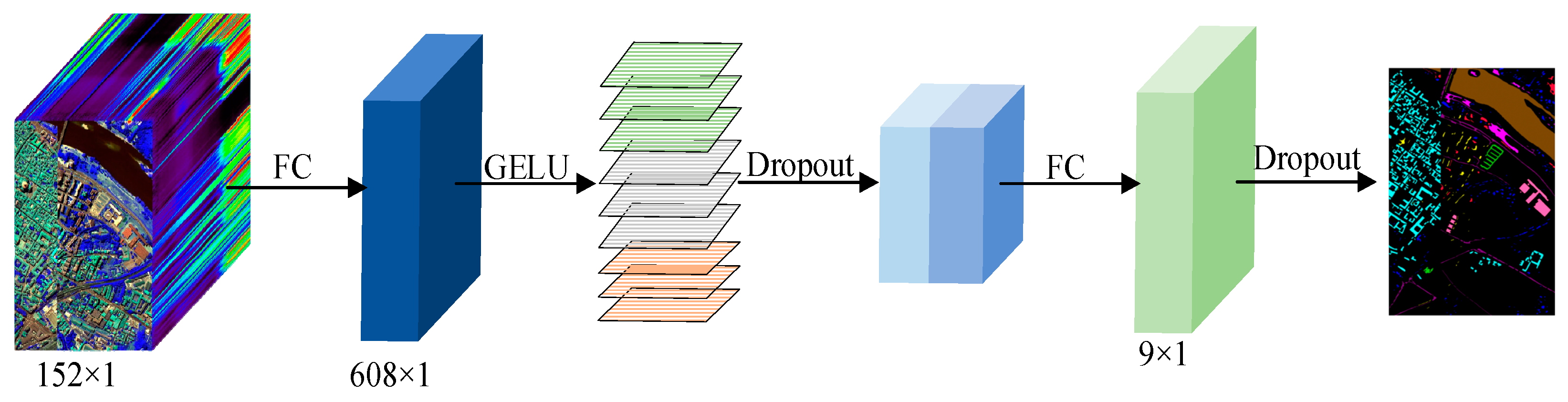
- We introduced a MLP model to further extract spectral-spatial features, eliminate the adverse effects of local connectivity of the model, pay more attention to the spatial structure information of the data, and improve the overall model’s anti-interference ability against noise.
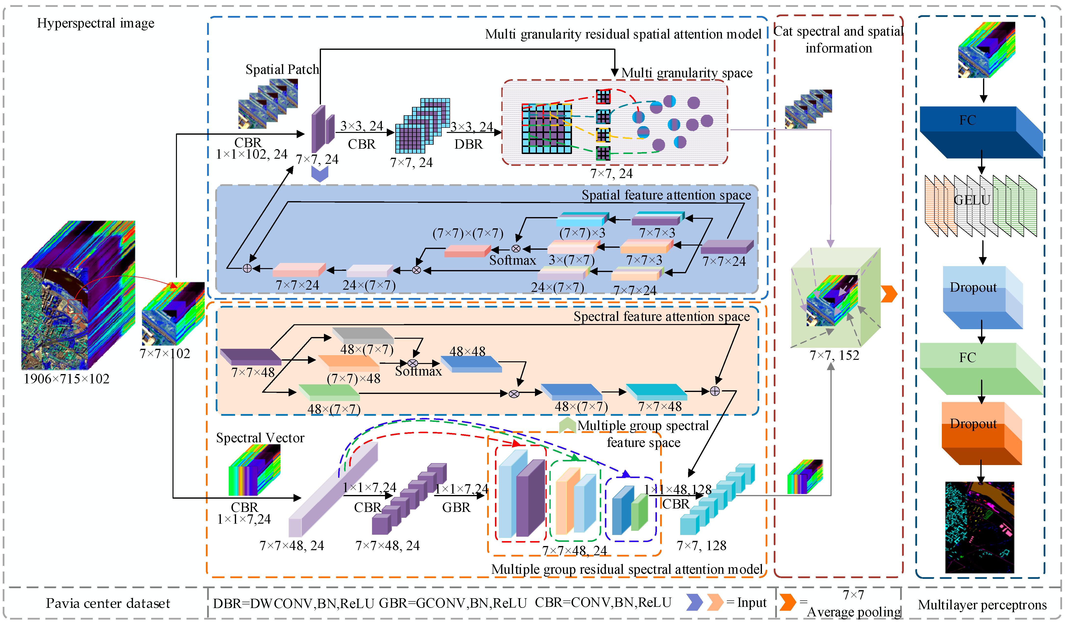
2. Methodology
2.1. Spectral and Spatial Feature Extraction
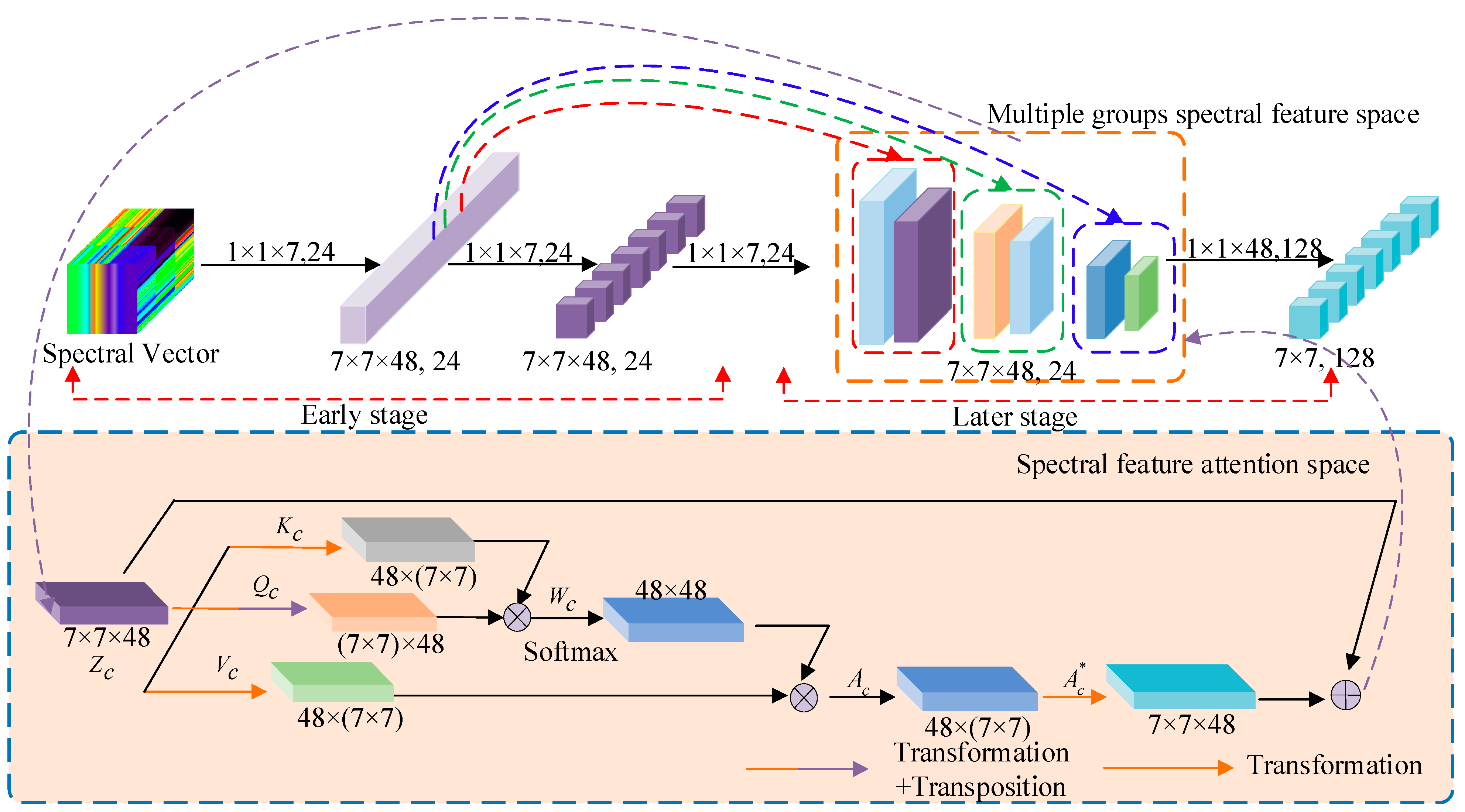
2.1.1. Spectral Feature Extraction
2.1.2. Spatial Feature Extraction
2.2. Spectral-Spatial Feature Extraction
2.3. Lion Optimization
3. Results
3.1. The Description of Public HSI Datasets
3.2. Experimental Setting
3.3. Classification Results of Different Methods
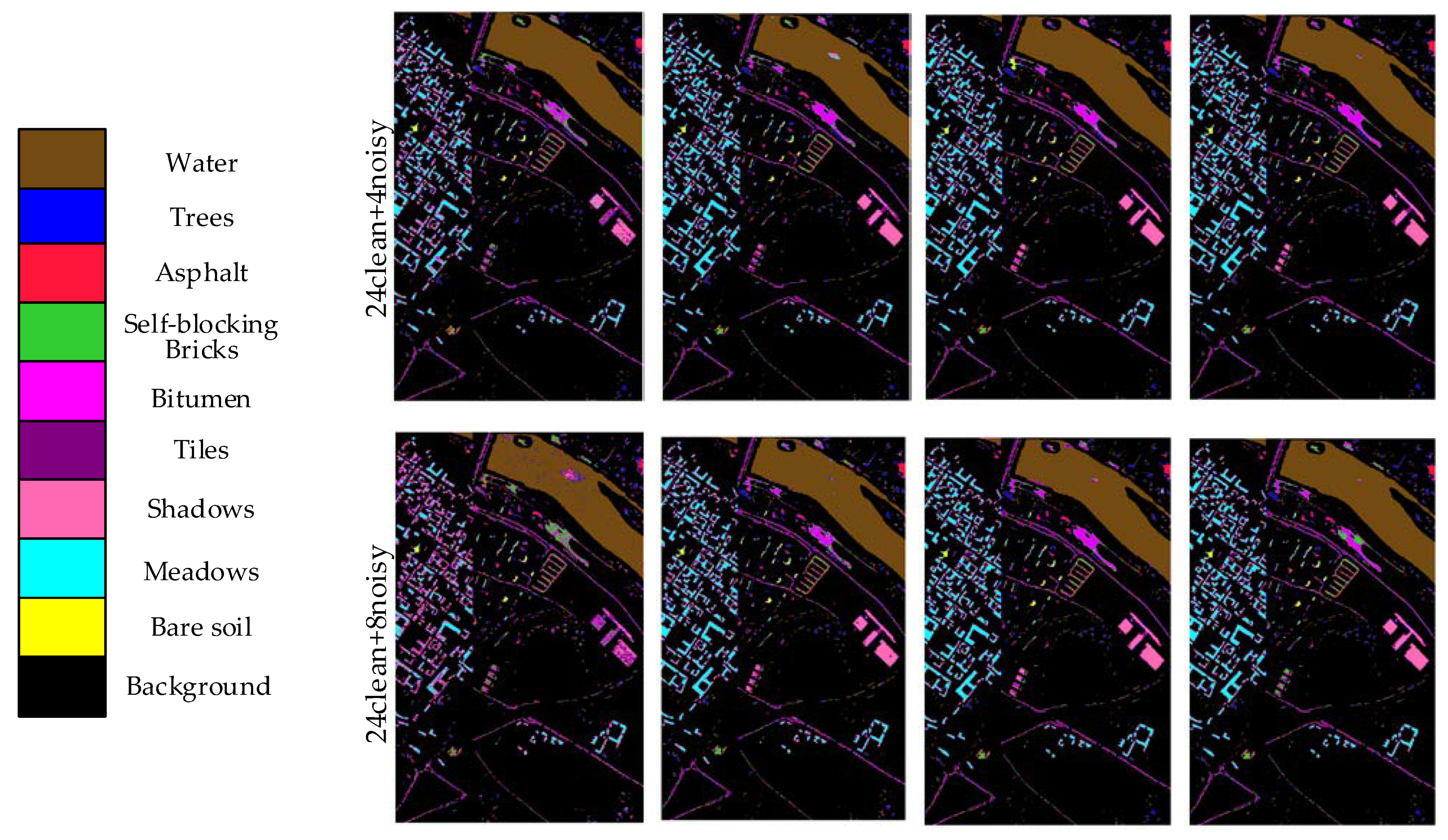
3.3.1. Results of PC Datasets with Different Numbers of Noise Samples
3.3.2. Results of LK Datasets with Different Numbers of Noise Samples
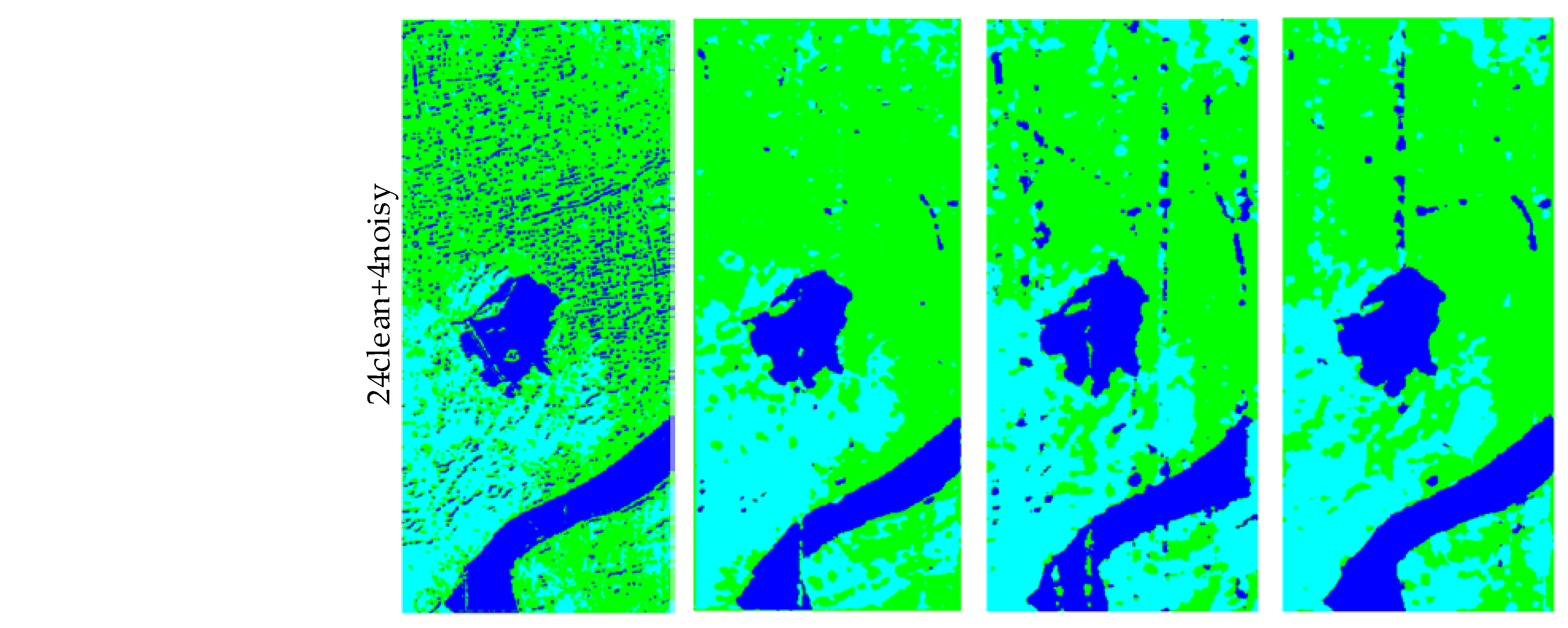
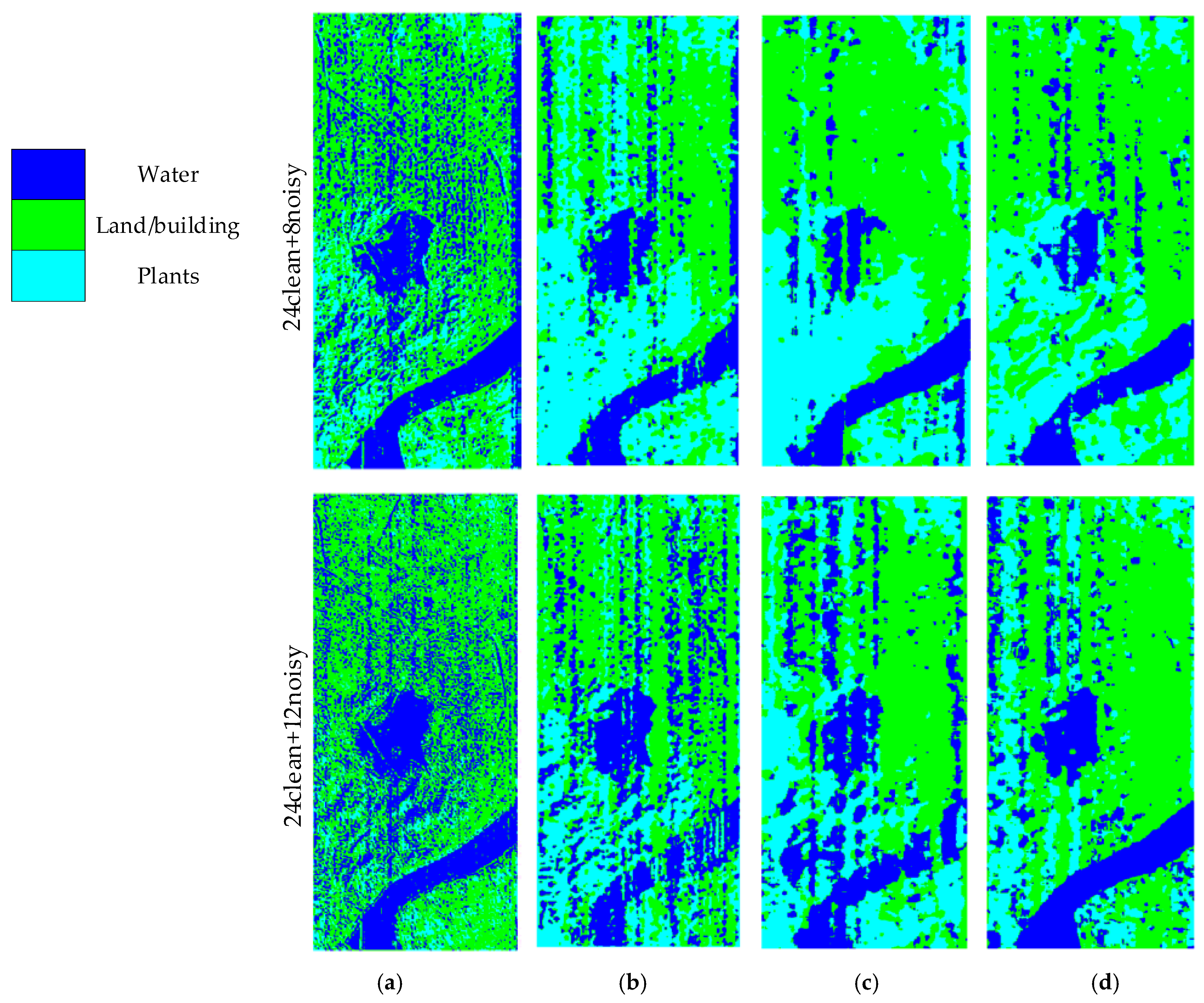
3.3.3. Results of HZ Datasets with Different Numbers of Noise Samples
3.4. The Numbers of Clean and Noisy Samples
3.5. Investigation of Running Time
4. Discussion
4.1. Effectiveness of the Attention Model
4.2. Effectiveness of the MLP Model
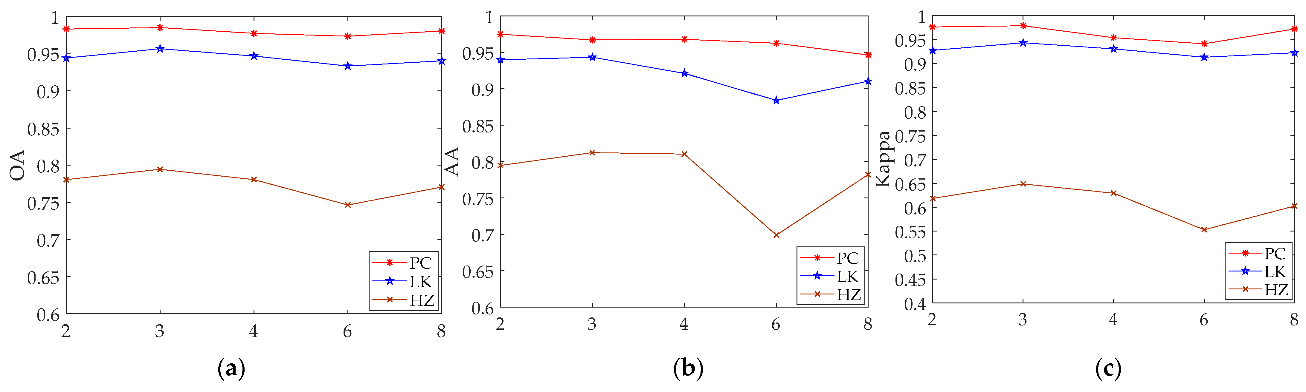
4.3. Effectiveness of the Number of Groups on the Model
5. Conclusions
Author Contributions
Funding
Data Availability Statement
Conflicts of Interest
References
- Paoletti, M.E.; Moreno-Álvarez, S.; Xue, Y.; Haut, J.M.; Plaza, A. AAtt-CNN: Automatic Attention-Based Convolutional Neural Networks for Hyperspectral Image Classification. IEEE Trans. Geosci. Remote Sens. 2023, 61, 5511118. [Google Scholar] [CrossRef]
- Qi, W.; Huang, C.; Wang, Y.; Zhang, X.; Sun, W.; Zhang, L. Global–Local 3-D Convolutional Transformer Network for Hyperspectral Image Classification. IEEE Trans. Geosci. Remote Sens. 2023, 61, 5510820. [Google Scholar] [CrossRef]
- Tu, B.; Ren, Q.; Li, Q.; He, W.; He, W. Hyperspectral Image Classification Using a Superpixel–Pixel–Subpixel Multilevel Network. IEEE Trans. Geosci. Remote Sens. 2023, 72, 5013616. [Google Scholar] [CrossRef]
- Weber, C.; Aguejdad, R.; Briottet, X.; Avala, J.; Fabre, S.; Demuynck, J.; Zenou, E.; Deville, Y.; Karoui, M.S.; Benhalouche, F.Z.; et al. Hyperspectral Imagery for Environmental Urban Planning. In Proceedings of the IGARSS 2018—2018 IEEE International Geoscience and Remote Sensing Symposium, Valencia, Spain, 22–27 July 2018; pp. 1628–1631. [Google Scholar]
- Yang, X.; Yu, Y. Estimating Soil Salinity Under Various Moisture Conditions: An Experimental Study. IEEE Trans. Geosci. Remote Sens. 2017, 55, 2525–2533. [Google Scholar] [CrossRef]
- Jiao, Q.; Zhang, B.; Liu, J.; Liu, L. A novel two-step method for winter wheat-leaf chlorophyll content estimation using a hyperspectral vegetation index. Int. J. Remote Sens. 2014, 35, 7363–7375. [Google Scholar] [CrossRef]
- Liang, L.; Di, L.; Zhang, L.; Deng, M.; Qin, Z.; Zhao, S.; Lin, H. Estimation of crop LAI using hyperspectral vegetation indices and a hybrid inversion method. Remote Sens. Environ. 2015, 165, 123–134. [Google Scholar] [CrossRef]
- Yue, J.; Fang, L.; Ghamisi, P.; Xie, W.; Li, J.; Chanussot, J.; Plaza, A. Optical Remote Sensing Image Understanding with Weak Supervision: Concepts, methods, and perspectives. IEEE Geosci. Remote Sens. Mag. 2022, 10, 250–269. [Google Scholar] [CrossRef]
- Pal, M.; Foody, G.M. Feature Selection for Classification of Hyperspectral Data by SVM. IEEE Trans. Geosci. Remote Sens. 2010, 48, 2297–2307. [Google Scholar] [CrossRef]
- Cui, M.; Prasad, S. Class-Dependent Sparse Representation Classifier for Robust Hyperspectral Image Classification. IEEE Trans. Geosci. Remote Sens. 2015, 53, 2683–2695. [Google Scholar] [CrossRef]
- Zheng, J.; Feng, Y.; Bai, C.; Zhang, J. Hyperspectral Image Classification Using Mixed Convolutions and Covariance Pooling. IEEE Trans. Geosci. Remote Sens. 2021, 59, 522–534. [Google Scholar] [CrossRef]
- Gu, Y.; Liu, T.; Jia, X.; Benediktsson, J.A.; Chanussot, J. Nonlinear Multiple Kernel Learning With Multiple-Structure-Element Extended Morphological Profiles for Hyperspectral Image Classification. IEEE Trans. Geosci. Remote Sens. 2016, 54, 3235–3247. [Google Scholar] [CrossRef]
- Liu, T.; Gu, Y.; Chanussot, J.; Dalla Mura, M. Multimorphological Superpixel Model for Hyperspectral Image Classification. IEEE Trans. Geosci. Remote Sens. 2017, 55, 6950–6963. [Google Scholar] [CrossRef]
- Hu, W.; Huang, Y.; Wei, L.; Zhang, F.; Li, H. Deep Convolutional Neural Networks for Hyperspectral Image Classification. J. Sens. 2015, 2015, 258619. [Google Scholar] [CrossRef]
- Mou, L.; Ghamisi, P.; Zhu, X.X. Deep recurrent neural networks for hyperspectral image classification. IEEE Trans. Geosci. Remote Sens. 2017, 55, 3639–3655. [Google Scholar] [CrossRef]
- Chen, Y.; Lin, Z.; Zhao, X.; Wang, G.; Gu, Y. Deep Learning-Based Classification of Hyperspectral Data. IEEE J. Sel. Top. Appl. Earth Obs. Remote Sens. 2014, 7, 2094–2107. [Google Scholar] [CrossRef]
- Fang, L.; Liu, G.; Li, S.; Ghamisi, P.; Benediktsson, J.A. Hyperspectral image classification with squeeze multibias network. IEEE Trans. Geosci. Remote Sens. 2019, 57, 1291–1301. [Google Scholar] [CrossRef]
- Feng, J.; Chen, J.; Sun, Q.; Shang, R.; Cao, X.; Zhang, X.; Jiao, L. Convolutional Neural Network Based on Bandwise-Independent Convolution and Hard Thresholding for Hyperspectral Band Selection. IEEE Trans. Cybern. 2021, 51, 4414–4428. [Google Scholar] [CrossRef]
- Kanthi, M.; Sarma, T.H.; Bindu, C.S. A 3d-Deep CNN Based Feature Extraction and Hyperspectral Image Classification. In Proceedings of the 2020 IEEE India Geoscience and Remote Sensing Symposium (InGARSS), Virtual, 1–4 December 2020; pp. 229–232. [Google Scholar]
- Wang, L.; Zhu, T.; Kumar, N.; Li, Z.; Wu, C.; Zhang, P. Attentive-Adaptive Network for Hyperspectral Images Classification With Noisy Labels. IEEE Trans. Geosci. Remote Sens. 2023, 61, 5505514. [Google Scholar] [CrossRef]
- Li, Y.F.; Guo, L.Z.; Zhou, Z.H. Towards Safe Weakly Supervised Learning. IEEE Trans. Pattern Anal. Mach. Intell. 2021, 43, 334–346. [Google Scholar] [CrossRef]
- Kang, X.; Duan, P.; Xiang, X.; Li, S.; Benediktsson, J.A. Detection and correction of mislabeled training samples for hyperspectral image classification. IEEE Trans. Geosci. Remote Sens. 2018, 56, 5673–5686. [Google Scholar] [CrossRef]
- Tu, B.; Zhang, X.; Kang, X.; Wang, J.; Benediktsson, J.A. Spatial density peak clustering for hyperspectral image classification with noisy labels. IEEE Trans. Geosci. Remote Sens. 2019, 57, 5085–5097. [Google Scholar] [CrossRef]
- Tu, B.; Zhou, C.; He, D.; Huang, S.; Plaza, A. Hyperspectral classification with noisy label detection via superpixel-to-pixel weighting distance. IEEE Trans. Geosci. Remote Sens. 2020, 58, 4116–4131. [Google Scholar] [CrossRef]
- Fang, Z.; Yang, Y.; Li, Z.; Li, W.; Chen, Y.; Ma, L.; Du, Q. Confident Learning-Based Domain Adaptation for Hyperspectral Image Classification. IEEE Trans. Geosci. Remote Sens. 2022, 60, 5527116. [Google Scholar] [CrossRef]
- Algan, G.; Ulusoy, I. Image classification with deep learning in the presence of noisy labels: A survey. Knowl.-Based Syst. 2021, 215, 106771–106790. [Google Scholar] [CrossRef]
- Roy, S.K.; Hong, D.; Kar, P.; Wu, X.; Liu, X.; Zhao, D. Lightweight heterogeneous kernel convolution for hyperspectral image classification with noisy labels. IEEE Geosci. Remote Sens. Lett. 2022, 19, 5509705. [Google Scholar] [CrossRef]
- Sukhbaatar, S.; Bruna, J.; Paluri, M.; Bourdev, L.; Fergus, R. Training convolutional networks with noisy labels. In Proceedings of the International Conference on Learning Representations, San Diego, CA, USA, 7–9 May 2015; pp. 1406–1427. [Google Scholar]
- Jiang, L.; Zhou, Z.; Leung, T.; Li, L.-J.; Li, F.-F. Mentornet:Learning data-driven curriculum for very deep neural networks on corrupted labels. In Proceedings of the International Conference on Machine Learning, Stockholm, Sweden, 10–15 July 2018; pp. 2304–2313. [Google Scholar]
- Xu, Y.; Li, Z.; Li, W.; Du, Q.; Liu, C.; Fang, Z.; Zhai, L. Dual-Channel Residual Network for Hyperspectral Image Classification with Noisy Labels. IEEE Trans. Geosci. Remote Sens. 2022, 60, 5502511. [Google Scholar] [CrossRef]
- Potghan, S.; Rajamenakshi, R.; Bhise, A. Multi-Layer Perceptron Based Lung Tumor Classification. In Proceedings of the 2018 Second International Conference on Electronics, Communication and Aerospace Technology (ICECA), Coimbatore, India, 29–31 March 2018; pp. 499–502. [Google Scholar]
- Chen, X.; Liang, C.; Huang, D.; Real, E.; Wang, K.; Liu, Y.; Pham, H.; Dong, X.; Luong, T.; Hsieh, C.; et al. Symbolic Discovery of Optimization Algorithms. arXiv 2023, arXiv:2302.06675v4. [Google Scholar]
- Li, Z.; Liu, M.; Chen, Y.; Xu, Y.; Li, W.; Du, Q. Deep Cross-Domain Few-Shot Learning for Hyperspectral Image Classification. IEEE Trans. Geosci. Remote Sens. 2022, 60, 5501618. [Google Scholar] [CrossRef]
- Zhong, Y.; Hu, X.; Luo, C.; Wang, X.; Zhao, J.; Zhang, L. WHU-Hi: UAV-borne hyperspectral with high spatial resolution (H2) benchmark datasets and classifier for precise crop identification based on deep convolutional neural network with CRF. Remote Sens. Environ. 2020, 250, 112012. [Google Scholar] [CrossRef]
- Deng, B.; Jia, S.; Shi, D. Deep Metric Learning-Based Feature Embedding for Hyperspectral Image Classification. IEEE Trans. Geosci. Remote Sens. 2020, 58, 1422–1435. [Google Scholar] [CrossRef]
- Gao, H.; Yang, Y.; Li, C.; Gao, L.; Zhang, B. Multiscale Residual Network With Mixed Depthwise Convolution for Hyperspectral Image Classification. IEEE Trans. Geosci. Remote Sens. 2021, 59, 3396–3408. [Google Scholar] [CrossRef]
- Roy, S.K.; Krishna, G.; Dubey, S.R.; Chaudhuri, B.B. HybridSN: Exploring 3-D–2-D CNN feature hierarchy for hyperspectral image classification. IEEE Geosci. Remote Sens. Lett. 2020, 17, 277–281. [Google Scholar] [CrossRef]
- Ying, L.; Haokui, Z.; Qiang, S. Spectral–Spatial Classification of Hyperspectral Imagery with 3D Convolutional Neural Network. Remote Sens. 2017, 9, 67. [Google Scholar]
- Zhong, Z.; Li, J.; .Luo, Z.; Chapman, M. Spectral–Spatial Residual Network for Hyperspectral Image Classification: A 3-D Deep Learning Framework. IEEE Trans. Geosci. Remote Sens. 2018, 56, 847–858. [Google Scholar] [CrossRef]


| Class | Class Name | Samples | Color | False-Color Map | Ground-Truth Map |
|---|---|---|---|---|---|
| C1 | Water | 65,971 |  |  | 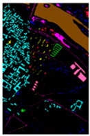 |
| C2 | Trees | 7598 |  | ||
| C3 | Asphalt | 3090 |  | ||
| C4 | Self-blocking Bricks | 2685 |  | ||
| C5 | Bitumen | 6584 |  | ||
| C6 | Tiles | 9248 |  | ||
| C7 | Shadows | 7287 |  | ||
| C8 | Meadows | 42,826 |  | ||
| C9 | Bare soil | 2863 |  | ||
| Background |  | ||||
| Total | 148,152 | ||||
| Class | Name | Samples | Color | False-Color Map | Ground-Truth Map |
|---|---|---|---|---|---|
| C1 | Corn | 34,511 |  | 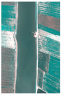 |  |
| C2 | Cotton | 8374 |  | ||
| C3 | Sesame | 3031 |  | ||
| C4 | Broad-leaf soybean | 63,212 |  | ||
| C5 | Narrow-leaf soybean | 4151 |  | ||
| C6 | Rice | 11,854 |  | ||
| C7 | Water | 67,056 |  | ||
| C8 | Roads and houses | 7124 |  | ||
| C9 | Mixed weed | 5229 |  | ||
| Background |  | ||||
| Total | 204,542 | ||||
| Class | Name | Samples | Color | False-Color Map | Ground-Truth Map |
|---|---|---|---|---|---|
| C1 | Water | 18,043 |  |  | 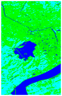 |
| C2 | Land/building | 77,450 |  | ||
| C3 | Plants | 40,207 |  | ||
| Total | 135,700 | ||||
| Class | DSNN | 2DCNN | 3DCNN | SSRN | DCRN | WSFL |
|---|---|---|---|---|---|---|
| C1 | 99.71 ± 0.09 | 99.60 ± 0.01 | 99.27 ± 0.49 | 99.73 ± 0.14 | 99.48 ± 0.10 | 99.81 ± 0.14 |
| C2 | 90.19 ± 9.44 | 82.21 ± 3.70 | 92.25 ± 1.80 | 94.51 ± 4.90 | 92.51 ± 1.97 | 91.82 ± 0.95 |
| C3 | 59.90 ± 12.25 | 95.21 ± 0.82 | 90.24 ± 3.44 | 98.19 ± 0.56 | 96.46 ± 0.35 | 97.92 ± 0.77 |
| C4 | 73.76 ± 9.60 | 73.91 ± 9.52 | 86.52 ± 7.75 | 99.77 ± 0.09 | 98.82 ± 0.17 | 99.71 ± 0.06 |
| C5 | 73.71 ± 10.33 | 86.72 ± 7.86 | 90.37 ± 2.94 | 85.84 ± 3.10 | 93.07 ± 1.83 | 97.59 ± 1.78 |
| C6 | 67.40 ± 12.41 | 99.22 ± 0.06 | 90.95 ± 4.59 | 99.21 ± 0.20 | 99.86 ± 0.10 | 98.52 ± 0.39 |
| C7 | 77.62 ± 5.93 | 67.45 ± 9.44 | 86.45 ± 3.79 | 97.36 ± 1.67 | 93.54 ± 5.03 | 95.39 ± 2.80 |
| C8 | 96.33 ± 0.98 | 99.07 ± 0.06 | 96.56 ± 2.16 | 99.46 ± 0.34 | 99.74 ± 0.11 | 99.51 ± 0.16 |
| C9 | 99.96 ± 0.09 | 100.00 ± 0.00 | 95.51 ± 0.98 | 100 ± 0.00 | 99.93 ± 0.01 | 98.42 ± 0.32 |
| OA (%) | 92.68 ± 1.81 | 95.87 ± 0.28 | 96.10 ± 0.43 | 98.60 ± 0.61 | 98.58 ± 0.27 | 98.84 ± 0.40 |
| AA (%) | 82.06 ± 3.26 | 89.26 ± 1.09 | 92.01 ± 0.54 | 97.11 ± 1.32 | 97.04 ± 0.66 | 97.75 ± 0.55 |
| Kappa | 89.56 ± 2.53 | 94.33 ± 0.39 | 94.54 ± 0.59 | 98.01 ± 0.86 | 98.01 ± 0.38 | 98.36 ± 0.32 |
| Class | DSNN | 2DCNN | 3DCNN | SSRN | DCRN | WSFL |
|---|---|---|---|---|---|---|
| C1 | 96.97 ± 2.58 | 87.62 ± 6.14 | 95.94 ± 2.51 | 97.51 ± 1.02 | 98.94 ± 0.09 | 92.62 ± 0.35 |
| C2 | 83.04 ± 10.08 | 68.48 ± 9.36 | 63.42 ± 8.84 | 94.97 ± 4.06 | 98.96 ± 0.92 | 99.27 ± 0.66 |
| C3 | 68.86 ± 11.83 | 73.83 ± 7.90 | 85.10 ± 3.90 | 99.54 ± 0.10 | 99.84 ± 0.12 | 99.92 ± 0.06 |
| C4 | 82.64 ± 10.30 | 70.87 ± 4.07 | 75.54 ± 1.52 | 86.71 ± 6.28 | 93.95 ± 2.23 | 98.12 ± 0.98 |
| C5 | 55.38 ± 16.30 | 56.25 ± 10.30 | 74.73 ± 7.86 | 97.63 ± 2.06 | 99.37 ± 0.50 | 97.82 ± 1.16 |
| C6 | 74.41 ± 6.93 | 90.11 ± 3.73 | 94.94 ± 4.08 | 99.07 ± 0.20 | 99.74 ± 0.08 | 99.13 ± 0.22 |
| C7 | 99.93 ± 0.01 | 99.92 ± 0.02 | 99.84 ± 0.07 | 99.72 ± 0.18 | 99.41 ± 0.15 | 99.56 ± 0.30 |
| C8 | 80.67 ± 12.56 | 89.15 ± 3.92 | 79.41 ± 4.48 | 95.38 ± 3.87 | 93.02 ± 2.92 | 96.97 ± 2.08 |
| C9 | 55.37 ± 13.39 | 72.96 ± 8.30 | 83.30 ± 2.53 | 95.44 ± 2.08 | 96.51 ± 1.53 | 96.04 ± 1.25 |
| OA (%) | 88.79 ± 1.26 | 84.67 ± 2.72 | 88.05 ± 1.61 | 94.77 ± 1.50 | 97.34 ± 0.59 | 97.69 ± 0.26 |
| AA (%) | 77.47 ± 6.92 | 78.79 ± 6.62 | 83.58 ± 3.34 | 96.21 ± 2.36 | 97.74 ± 0.39 | 97.71 ± 0.51 |
| Kappa | 85.39 ± 1.47 | 80.70 ± 3.37 | 84.71 ± 2.06 | 93.25 ± 1.89 | 96.52 ± 0.77 | 96.86 ± 0.33 |
| Class | DSNN | 2DCNN | 3DCNN | SSRN | DCRN | WSFL |
|---|---|---|---|---|---|---|
| C1 | 81.10 ± 4.16 | 88.68 ± 2.65 | 93.92 ± 2.85 | 88.62 ± 1.73 | 89.30 ± 1.15 | 91.79 ± 1.29 |
| C2 | 64.96 ± 10.71 | 71.94 ± 5.08 | 70.71 ± 2.67 | 74.35 ± 3.47 | 76.35 ± 4.63 | 77.25 ± 4.87 |
| C3 | 98.65 ± 0.60 | 73.11 ± 10.52 | 79.57 ± 3.47 | 84.20 ± 1.09 | 81.32 ± 6.31 | 80.79 ± 2.98 |
| OA (%) | 77.07 ± 7.99 | 74.54 ± 4.80 | 76.41 ± 1.48 | 79.17 ± 2.00 | 79.52 ± 1.21 | 80.23 ± 1.82 |
| AA (%) | 81.57 ± 3.76 | 77.91 ± 1.39 | 81.40 ± 1.06 | 82.39 ± 1.01 | 82.32 ± 0.95 | 83.27 ± 0.80 |
| Kappa | 62.51 ± 10.40 | 59.19 ± 4.75 | 60.66 ± 2.32 | 64.95 ± 3.05 | 65.41 ± 1.77 | 66.51 ± 2.19 |
| Class | The Number of Clean and Noisy Training Samples | |||||||||||
|---|---|---|---|---|---|---|---|---|---|---|---|---|
| 24(clean) + 4(noisy) | 24(clean) + 8(noisy) | 24(clean) + 12(noisy) | ||||||||||
| 3DCNN | SSRN | DCRN | WSFL | 3DCNN | SSRN | DCRN | WSFL | 3DCNN | SSRN | DCRN | WSFL | |
| C1 Std | 98.33 0.84 | 98.88 0.54 | 98.35 0.53 | 99.87 0.12 | 94.07 3.70 | 97.32 1.39 | 97.49 1.31 | 99.53 0.15 | 86.15 3.39 | 94.56 4.10 | 98.14 0.12 | 98.23 0.10 |
| C2 Std | 82.22 1.62 | 94.75 2.46 | 93.13 2.84 | 96.00 2.47 | 70.41 3.62 | 91.17 4.99 | 92.51 3.03 | 91.07 2.81 | 54.34 10.35 | 89.30 6.78 | 91.00 4.53 | 92.83 2.39 |
| C3 Std | 82.15 2.41 | 89.77 6.92 | 91.70 0.48 | 90.74 1.46 | 74.38 5.95 | 87.84 6.90 | 94.12 1.98 | 94.22 1.30 | 62.42 12.65 | 63.44 4.71 | 93.89 2.30 | 86.32 3.50 |
| C4 Std | 79.01 3.59 | 95.62 1.63 | 96.28 3.21 | 98.81 1.08 | 52.66 3.15 | 88.30 7.29 | 91.01 4.08 | 97.99 1.42 | 44.74 1.73 | 91.00 8.79 | 94.50 2.29 | 92.34 3.25 |
| C5 Std | 75.53 6.29 | 92.55 3.30 | 96.29 2.67 | 96.91 2.33 | 62.45 10.71 | 92.59 2.33 | 89.34 1.74 | 91.02 2.27 | 47.53 10.01 | 85.03 8.64 | 92.03 4.32 | 92.04 2.91 |
| C6 Std | 81.60 7.80 | 94.42 2.05 | 96.04 1.06 | 98.21 0.74 | 62.99 8.02 | 89.92 2.37 | 98.96 0.76 | 98.28 1.25 | 50.35 3.66 | 81.70 1.94 | 95.73 2.62 | 98.33 1.22 |
| C7 Std | 72.25 2.43 | 94.70 3.28 | 94.78 1.07 | 92.42 1.95 | 61.85 5.57 | 91.19 4.77 | 93.62 1.07 | 90.81 1.92 | 52.28 9.03 | 77.83 5.02 | 93.59 2.06 | 91.84 2.37 |
| C8 Std | 83.54 6.46 | 91.24 0.61 | 97.06 1.25 | 98.77 0.19 | 68.04 4.14 | 91.69 1.59 | 96.48 2.09 | 97.54 0.32 | 56.75 4.26 | 90.38 2.47 | 93.28 5.06 | 97.49 1.00 |
| C9 Std | 91.95 7.20 | 97.60 1.46 | 98.39 0.32 | 98.67 0.58 | 79.55 8.09 | 95.94 3.72 | 99.57 0.13 | 99.62 0.07 | 75.85 6.19 | 87.68 7.12 | 91.16 5.91 | 96.36 2.13 |
| OA(%) Std | 89.09 2.79 | 95.42 0.28 | 97.12 0.80 | 98.52 0.45 | 78.98 3.93 | 94.02 0.95 | 96.34 1.95 | 97.50 0.12 | 68.98 2.00 | 90.20 2.56 | 95.44 3.82 | 96.77 0.71 |
| AA(%) Std | 82.95 2.53 | 94.39 1.31 | 95.78 1.60 | 96.71 1.34 | 69.60 3.50 | 91.77 1.21 | 94.79 0.79 | 95.57 0.40 | 58.93 1.31 | 84.55 0.70 | 93.70 4.42 | 93.97 1.81 |
| Kappa Std | 84.82 3.68 | 93.69 0.40 | 95.82 1.13 | 97.91 0.64 | 71.44 4.85 | 91.68 1.31 | 94.87 2.61 | 96.48 0.17 | 58.64 1.21 | 86.40 3.33 | 93.62 5.99 | 95.48 1.00 |
| Class | The Number of Clean and Noisy Training Samples | |||||||||||
|---|---|---|---|---|---|---|---|---|---|---|---|---|
| 24(clean) + 4(noisy) | 24(clean) + 8(noisy) | 24(clean) + 12(noisy) | ||||||||||
| 3DCNN | SSRN | DCRN | WSFL | 3DCNN | SSRN | DCRN | WSFL | 3DCNN | SSRN | DCRN | WSFL | |
| C1 Std | 79.28 9.23 | 94.03 1.45 | 95.79 2.22 | 94.97 1.13 | 60.90 9.68 | 88.49 4.86 | 90.38 4.84 | 94.18 3.62 | 50.76 7.42 | 80.23 1.41 | 87.94 4.02 | 92.46 3.20 |
| C2 Std | 47.53 7.56 | 92.53 4.32 | 89.40 5.61 | 92.86 2.45 | 44.77 7.54 | 79.26 11.0 | 90.30 7.06 | 81.54 2.97 | 46.53 3.98 | 74.26 7.27 | 86.31 8.84 | 82.57 4.42 |
| C3 Std | 67.64 8.18 | 91.49 1.60 | 98.63 0.81 | 97.73 1.93 | 55.33 10.02 | 90.50 5.67 | 89.52 5.90 | 90.73 3.41 | 50.34 7.55 | 83.88 4.73 | 86.63 9.83 | 91.29 5.49 |
| C4 Std | 61.17 6.26 | 89.50 5.24 | 91.42 4.13 | 93.33 5.07 | 48.21 6.79 | 83.85 5.38 | 81.86 6.45 | 82.05 4.49 | 42.85 3.18 | 79.11 5.57 | 77.52 3.02 | 76.35 2.35 |
| C5 Std | 64.15 9.81 | 89.74 3.60 | 89.20 4.23 | 94.42 1.27 | 44.40 6.80 | 83.49 8.73 | 86.42 6.79 | 91.07 3.85 | 45.92 10.05 | 75.83 7.76 | 81.88 8.45 | 88.31 7.01 |
| C6 Std | 82.62 7.59 | 96.51 1.60 | 98.55 1.06 | 94.13 1.20 | 62.05 6.20 | 92.57 5.34 | 91.83 3.24 | 93.86 1.17 | 57.35 8.55 | 89.79 5.14 | 80.19 6.15 | 82.72 4.55 |
| C7 Std | 98.63 0.49 | 98.20 1.06 | 98.38 0.66 | 99.70 0.02 | 96.11 0.83 | 97.11 1.98 | 98.23 0.55 | 99.57 0.18 | 92.59 1.20 | 95.01 4.96 | 96.64 2.31 | 99.32 0.29 |
| C8 Std | 71.44 3.38 | 87.52 4.91 | 91.45 2.54 | 92.34 1.91 | 58.44 7.05 | 77.55 7.59 | 82.76 7.60 | 83.93 3.60 | 52.18 2.46 | 70.39 8.34 | 76.85 11.07 | 78.51 8.09 |
| C9 Std | 57.81 10.65 | 88.09 3.83 | 89.36 1.06 | 89.52 2.71 | 47.52 6.75 | 77.32 3.51 | 82.75 4.12 | 80.71 2.50 | 42.77 6.20 | 70.33 5.61 | 73.01 6.31 | 75.50 2.55 |
| OA(%) Std | 77.63 3.92 | 93.58 2.00 | 94.78 1.42 | 95.68 0.71 | 67.09 3.80 | 89.01 2.85 | 89.85 3.01 | 90.85 1.58 | 61.99 2.87 | 84.42 2.06 | 86.15 3.73 | 87.74 1.85 |
| AA(%) Std | 70.03 4.46 | 91.96 1.07 | 93.58 1.25 | 94.33 1.06 | 57.52 2.50 | 85.57 2.82 | 88.23 3.87 | 88.63 2.26 | 53.48 4.25 | 79.87 0.32 | 83.00 4.42 | 85.23 2.78 |
| Kappa Std | 71.73 4.72 | 91.67 2.53 | 93.22 1.82 | 94.36 0.88 | 58.94 4.47 | 85.82 3.62 | 86.89 3.78 | 88.18 2.01 | 53.07 3.48 | 79.98 2.49 | 82.23 4.64 | 84.28 2.39 |
| Class | The Number of Clean and Noisy Training Samples | |||||||||||
|---|---|---|---|---|---|---|---|---|---|---|---|---|
| 24(clean) + 4(noisy) | 24(clean) + 8(noisy) | 24(clean) + 12(noisy) | ||||||||||
| 3DCNN | SSRN | DCRN | WSFL | 3DCNN | SSRN | DCRN | WSFL | 3DCNN | SSRN | DCRN | WSFL | |
| C1 Std | 86.43 4.55 | 81.07 9.46 | 81.43 4.13 | 88.37 3.86 | 77.53 5.09 | 71.54 8.98 | 73.39 5.81 | 83.05 3.34 | 77.06 4.86 | 75.88 8.70 | 69.43 7.41 | 81.33 3.20 |
| C2 Std | 71.20 5.98 | 79.61 5.96 | 76.85 5.35 | 78.97 2.24 | 60.06 8.90 | 58.05 5.60 | 64.80 3.49 | 73.07 2.39 | 51.85 8.49 | 57.98 9.17 | 59.52 8.70 | 62.45 4.57 |
| C3 Std | 76.26 2.13 | 70.40 8.89 | 77.03 7.67 | 76.35 3.26 | 62.12 7.36 | 75.63 5.30 | 67.95 7.68 | 68.03 3.82 | 65.33 8.46 | 60.75 9.60 | 64.51 8.10 | 57.76 4.37 |
| OA(%) Std | 74.72 3.90 | 77.07 5.51 | 77.51 2.87 | 79.44 1.19 | 62.99 6.17 | 65.05 3.31 | 66.88 2.58 | 72.90 1.96 | 59.19 6.37 | 61.18 3.62 | 62.31 3.42 | 63.57 3.28 |
| AA(%) Std | 77.96 2.78 | 77.03 6.04 | 78.44 2.90 | 81.23 1.86 | 66.57 4.28 | 68.41 1.70 | 68.71 1.40 | 74.72 0.94 | 64.75 4.90 | 64.87 1.52 | 64.49 2.04 | 67.18 2.02 |
| Kappa Std | 57.61 5.95 | 60.30 8.62 | 61.49 4.39 | 64.84 2.29 | 40.81 8.50 | 44.08 4.15 | 68.71 3.52 | 54.69 2.39 | 36.00 8.62 | 37.42 2.94 | 39.46 3.90 | 40.32 3.01 |
| Class | The Numbers of Clean and Noisy Training Samples | |||||||||||
|---|---|---|---|---|---|---|---|---|---|---|---|---|
| 8(clean) + 4(noisy) | 8 (clean) + 8(noisy) | 8(clean) + 12(noisy) | ||||||||||
| 3DCNN | SSRN | DCRN | WSFL | 3DCNN | SSRN | DCRN | WSFL | 3DCNN | SSRN | DCRN | WSFL | |
| OA(%) Std | 67.60 3.91 | 84.09 4.80 | 90.96 4.61 | 94.02 3.03 | 52.78 4.96 | 79.55 3.04 | 82.05 5.41 | 85.92 4.61 | 41.50 5.11 | 61.68 4.97 | 67.08 8.72 | 71.35 7.16 |
| AA(%) Std | 57.81 7.67 | 79.92 7.97 | 84.36 3.06 | 86.78 3.21 | 42.80 5.97 | 70.72 3.57 | 67.39 3.63 | 85.26 2.79 | 32.65 5.08 | 55.81 1.63 | 57.90 6.96 | 64.29 6.02 |
| Kappa Std | 57.05 5.15 | 79.01 6.47 | 87.35 6.21 | 91.53 4.05 | 40.60 4.71 | 72.31 3.36 | 75.21 7.14 | 80.74 5.14 | 27.63 5.22 | 50.26 5.45 | 56.60 10.37 | 62.51 8.15 |
| 20(clean) + 4(noisy) | 20(clean) + 8(noisy) | 20(clean) + 12(noisy) | ||||||||||
| 3DCNN | SSRN | DCRN | WSFL | 3DCNN | SSRN | DCRN | WSFL | 3DCNN | SSRN | DCRN | WSFL | |
| OA(%) Std | 82.16 2.50 | 94.41 0.81 | 96.76 0.61 | 97.61 0.94 | 73.48 0.46 | 93.36 1.55 | 93.92 3.77 | 96.63 2.05 | 62.58 3.92 | 86.14 1.06 | 91.82 6.25 | 96.38 2.43 |
| AA(%) Std | 73.83 2.56 | 92.68 1.85 | 95.17 0.86 | 94.04 1.22 | 63.30 1.01 | 89.16 1.44 | 89.89 3.49 | 94.65 1.77 | 54.09 1.67 | 79.85 1.88 | 88.01 6.64 | 93.49 3.01 |
| Kappa Std | 75.58 3.44 | 92.15 1.15 | 95.43 0.87 | 96.61 1.32 | 64.24 0.30 | 90.69 2.10 | 91.51 5.12 | 95.25 2.80 | 51.74 4.43 | 81.00 1.44 | 88.69 8.54 | 94.89 3.39 |
| 24(clean) + 4(noisy) | 24(clean) + 8(noisy) | 24(clean) + 12(noisy) | ||||||||||
| 3DCNN | SSRN | DCRN | WSFL | 3DCNN | SSRN | DCRN | WSFL | 3DCNN | SSRN | DCRN | WSFL | |
| OA(%) Std | 89.09 2.79 | 95.42 0.28 | 97.12 0.80 | 98.52 0.45 | 78.98 3.93 | 94.02 0.95 | 96.34 1.95 | 97.50 0.12 | 68.98 2.00 | 90.20 2.56 | 95.44 3.82 | 96.77 0.71 |
| AA(%) Std | 82.95 2.53 | 94.39 1.31 | 95.78 1.60 | 96.71 1.34 | 69.60 3.50 | 91.77 1.21 | 94.79 0.79 | 95.57 0.40 | 58.93 1.31 | 84.55 0.70 | 93.70 4.42 | 93.97 1.81 |
| Kappa Std | 84.82 3.68 | 93.69 0.40 | 95.82 1.13 | 97.91 0.64 | 71.44 4.85 | 91.68 1.31 | 94.87 2.61 | 96.48 0.17 | 58.64 1.21 | 86.40 3.33 | 93.62 5.99 | 95.48 1.00 |
| Metrics | The Numbers of Clean and Noisy Training Samples | |||||||||||
|---|---|---|---|---|---|---|---|---|---|---|---|---|
| 8(clean) + 4(noisy) | 8 (clean) + 8(noisy) | 8(clean) + 12(noisy) | ||||||||||
| 3DCNN | SSRN | DCRN | WSFL | 3DCNN | SSRN | DCRN | WSFL | 3DCNN | SSRN | DCRN | WSFL | |
| OA(%) Std | 58.65 2.84 | 80.42 3.72 | 80.58 5.35 | 84.63 3.39 | 51.42 5.28 | 66.12 7.23 | 66.40 4.74 | 68.17 3.79 | 45.25 4.54 | 55.71 5.47 | 56.87 3.71 | 60.93 3.54 |
| AA(%) Std | 46.53 2.73 | 74.66 2.33 | 78.51 1.67 | 78.45 2.86 | 36.50 4.83 | 60.84 4.15 | 65.69 3.18 | 66.81 4.05 | 32.91 2.73 | 47.92 4.81 | 51.97 3.09 | 52.57 2.62 |
| Kappa Std | 49.13 2.96 | 75.17 4.38 | 75.55 6.37 | 80.39 4.02 | 40.69 6.01 | 58.16 8.04 | 58.63 5.56 | 60.50 4.02 | 34.25 4.61 | 46.18 5.94 | 47.02 3.93 | 52.10 3.74 |
| Metrics | 20(clean) + 4(noisy) | 20(clean) + 8(noisy) | 20(clean) + 12(noisy) | |||||||||
| 3DCNN | SSRN | DCRN | WSFL | 3DCNN | SSRN | DCRN | WSFL | 3DCNN | SSRN | DCRN | WSFL | |
| OA(%) Std | 69.08 2.20 | 87.52 4.74 | 92.12 2.60 | 94.83 1.74 | 66.98 3.09 | 79.70 3.76 | 87.63 6.29 | 89.54 2.79 | 55.47 5.70 | 74.68 6.44 | 81.10 5.51 | 85.21 2.52 |
| AA(%) Std | 61.24 3.14 | 86.80 1.20 | 91.58 1.19 | 92.19 1.06 | 55.51 1.02 | 77.96 3.49 | 85.63 4.33 | 88.54 2.15 | 45.17 5.82 | 70.92 3.57 | 79.17 6.98 | 80.63 2.97 |
| Kappa Std | 61.44 2.56 | 84.03 5.58 | 89.82 3.31 | 93.27 2.22 | 58.50 3.37 | 74.53 4.69 | 84.10 7.87 | 86.41 3.57 | 45.17 6.63 | 68.13 7.64 | 76.02 7.04 | 81.07 3.06 |
| Metrics | 24(clean) + 4(noisy) | 24(clean) + 8(noisy) | 24(clean) + 12(noisy) | |||||||||
| 3DCNN | SSRN | DCRN | WSFL | 3DCNN | SSRN | DCRN | WSFL | 3DCNN | SSRN | DCRN | WSFL | |
| OA(%) Std | 77.63 3.92 | 93.58 2.00 | 94.78 1.42 | 95.68 0.71 | 67.09 3.80 | 89.01 2.85 | 89.85 3.01 | 90.85 1.58 | 61.99 2.87 | 84.42 2.06 | 86.15 3.73 | 87.74 1.85 |
| AA(%) Std | 70.03 4.46 | 91.96 1.07 | 93.58 1.25 | 94.33 1.06 | 57.52 2.50 | 85.57 2.82 | 88.23 3.87 | 88.63 2.26 | 53.48 4.25 | 79.87 0.32 | 83.00 4.42 | 85.23 2.78 |
| Kappa Std | 71.73 4.72 | 91.67 2.53 | 93.22 1.82 | 94.36 0.88 | 58.94 4.47 | 85.82 3.62 | 86.89 3.78 | 88.18 2.01 | 53.07 3.48 | 79.98 2.49 | 82.23 4.64 | 84.28 2.39 |
| Metrics | The Numbers of Clean and Noisy Training Samples | |||||||||||
|---|---|---|---|---|---|---|---|---|---|---|---|---|
| 8(clean) + 4(noisy) | 8(clean) + 8(noisy) | 8(clean) + 12(noisy) | ||||||||||
| 3DCNN | SSRN | DCRN | WSFL | 3DCNN | SSRN | DCRN | WSFL | 3DCNN | SSRN | DCRN | WSFL | |
| OA(%) Std | 58.03 4.59 | 62.36 5.29 | 62.82 7.45 | 66.26 5.06 | 41.66 5.94 | 44.89 4.76 | 48.66 8.29 | 54.97 3.30 | 35.53 8.79 | 35.68 4.51 | 36.60 6.92 | 43.34 5.26 |
| AA(%) Std | 63.96 3.85 | 62.26 3.84 | 67.65 7.73 | 65.43 5.74 | 46.75 6.77 | 47.44 7.91 | 50.83 10.2 | 63.48 3.62 | 38.35 6.02 | 36.71 5.41 | 40.64 7.52 | 40.23 4.79 |
| Kappa Std | 34.77 6.43 | 38.11 6.51 | 42.32 10.5 | 44.69 6.12 | 10.06 8.20 | 16.30 7.94 | 21.04 11.3 | 32.64 4.89 | 5.82 4.46 | 6.44 4.95 | 7.36 8.21 | 11.18 4.47 |
| Metrics | 20(clean) + 4(noisy) | 20(clean) + 8(noisy) | 20(clean) + 12(noisy) | |||||||||
| 3DCNN | SSRN | DCRN | WSFL | 3DCNN | SSRN | DCRN | WSFL | 3DCNN | SSRN | DCRN | WSFL | |
| OA(%) Std | 68.35 4.25 | 71.09 6.25 | 73.21 5.03 | 77.64 4.71 | 58.25 3.25 | 64.82 4.67 | 65.64 5.48 | 66.62 4.94 | 58.03 3.72 | 59.73 4.73 | 61.70 4.47 | 61.96 3.27 |
| AA(%) Std | 71.75 2.43 | 75.48 3.69 | 75.65 2.70 | 80.65 2.55 | 63.30 3.40 | 68.48 2.11 | 70.13 3.96 | 70.96 3.09 | 62.53 2.70 | 61.21 2.43 | 62.39 4.54 | 65.68 3.97 |
| Kappa Std | 49.23 6.00 | 52.84 7.93 | 55.43 6.27 | 62.26 5.71 | 33.69 4.90 | 43.07 5.91 | 70.13 7.71 | 45.84 5.49 | 33.84 5.36 | 34.69 5.33 | 37.66 6.36 | 38.13 4.82 |
| Metrics | 24(clean) + 4(noisy) | 24(clean) + 8(noisy) | 24(clean) + 12(noisy) | |||||||||
| 3DCNN | SSRN | DCRN | WSFL | 3DCNN | SSRN | DCRN | WSFL | 3DCNN | SSRN | DCRN | WSFL | |
| OA(%) Std | 74.72 3.90 | 77.07 5.51 | 77.51 2.87 | 79.44 1.19 | 62.99 6.17 | 65.05 3.31 | 66.88 2.58 | 72.90 1.96 | 59.19 6.37 | 61.18 3.62 | 62.31 3.42 | 63.57 3.28 |
| AA(%) Std | 77.96 2.78 | 77.03 6.04 | 78.44 2.90 | 81.23 1.86 | 66.57 4.28 | 68.41 1.70 | 68.71 1.40 | 74.72 0.94 | 64.75 4.90 | 64.87 1.52 | 64.49 2.04 | 67.18 2.02 |
| Kappa Std | 57.61 5.95 | 60.30 8.62 | 61.49 4.39 | 64.84 2.29 | 40.81 8.50 | 44.08 4.15 | 68.71 3.52 | 54.69 2.39 | 36.00 8.62 | 37.42 2.94 | 39.46 3.90 | 40.32 2.39 |
| Algorithm | DSNN | 2DCNN | 3DCNN | SSRN | DCRN | WSFL | |
|---|---|---|---|---|---|---|---|
| Dataset | |||||||
| Pavia Center | 203.60 | 207.69 | 161.21 | 241.27 | 273.14 | 268.67 | |
| WHU-Hi-LongKou | 89.74 | 84.97 | 298.79 | 390.17 | 330.76 | 375.81 | |
| HangZhou | 56.06 | 55.83 | 118.26 | 151.64 | 151.92 | 158.27 | |
| Algorithm | Index | MGRSAM | MRSAM | MGRSAM + MRSAM | |
|---|---|---|---|---|---|
| Dataset | |||||
| Pavia Center | OA | 98.27 | 98.26 | 98.52 | |
| AA | 96.47 | 96.54 | 96.71 | ||
| Kappa | 97.55 | 97.54 | 97.91 | ||
| WHU-Hi-LongKou | OA | 95.34 | 95.28 | 95.68 | |
| AA | 91.02 | 94.59 | 94.33 | ||
| Kappa | 93.93 | 93.86 | 94.36 | ||
| HangZhou | OA | 77.78 | 78.91 | 79.44 | |
| AA | 79.14 | 80.13 | 81.23 | ||
| Kappa | 62.01 | 81.23 | 64.84 | ||
| Algorithm | Index | Without MLP | With MLP | |
|---|---|---|---|---|
| Dataset | ||||
| Pavia Center | OA | 98.23 | 98.52 | |
| AA | 96.34 | 96.71 | ||
| Kappa | 97.50 | 97.91 | ||
| WHU-Hi-LongKou | OA | 95.01 | 95.68 | |
| AA | 94.11 | 94.33 | ||
| Kappa | 93.21 | 94.36 | ||
| HangZhou | OA | 78.48 | 79.44 | |
| AA | 78.38 | 81.23 | ||
| Kappa | 62.06 | 64.84 | ||
Disclaimer/Publisher’s Note: The statements, opinions and data contained in all publications are solely those of the individual author(s) and contributor(s) and not of MDPI and/or the editor(s). MDPI and/or the editor(s) disclaim responsibility for any injury to people or property resulting from any ideas, methods, instructions or products referred to in the content. |
© 2023 by the authors. Licensee MDPI, Basel, Switzerland. This article is an open access article distributed under the terms and conditions of the Creative Commons Attribution (CC BY) license (https://creativecommons.org/licenses/by/4.0/).
Share and Cite
Liu, C.; Zhao, L.; Wu, H. Hyperspectral Images Weakly Supervised Classification with Noisy Labels. Remote Sens. 2023, 15, 4994. https://doi.org/10.3390/rs15204994
Liu C, Zhao L, Wu H. Hyperspectral Images Weakly Supervised Classification with Noisy Labels. Remote Sensing. 2023; 15(20):4994. https://doi.org/10.3390/rs15204994
Chicago/Turabian StyleLiu, Chengyang, Lin Zhao, and Haibin Wu. 2023. "Hyperspectral Images Weakly Supervised Classification with Noisy Labels" Remote Sensing 15, no. 20: 4994. https://doi.org/10.3390/rs15204994
APA StyleLiu, C., Zhao, L., & Wu, H. (2023). Hyperspectral Images Weakly Supervised Classification with Noisy Labels. Remote Sensing, 15(20), 4994. https://doi.org/10.3390/rs15204994