Spatial Prediction of Landslide Susceptibility Using Logistic Regression (LR), Functional Trees (FTs), and Random Subspace Functional Trees (RSFTs) for Pengyang County, China

Abstract

Landslides pose significant and serious geological threat disasters worldwide, threatening human lives and property; China is particularly susceptible to these disasters. This paper focuses on Pengyang County, which is situated in the Ningxia Hui Autonomous Region of China, an area prone to landslides. This study investigated the application of machine learning techniques for analyzing landslide susceptibility. To construct and validate the model, we initially compiled a landslide inventory comprising 972 historical landslides and an equivalent number of non-landslide sites (Data sourced from the Pengyang County Department of Natural Resources). To ensure an impartial evaluation, both the landslide and non-landslide datasets were randomly divided into two sets using a 70/30 ratio. Next, we extracted 15 landslide conditioning factors, including the slope angle, elevation, profile curvature, plan curvature, slope aspect, TWI (topographic wetness index), TPI (topographic position index), distance to roads and rivers, NDVI (normalized difference vegetation index), rainfall, land use, lithology, SPI (stream power index), and STI (sediment transport index), from the spatial database. Subsequently, a correlation analysis between the conditioning factors and landslide occurrences was conducted using the certainty factor (CF) method. Three landslide models were established by employing logistic regression (LR), functional trees (FTs), and random subspace functional trees (RSFTs) algorithms. The landslide susceptibility map was categorized into five levels: very low, low, medium, high, and very high susceptibility. Finally, the predictive capability of the three algorithms was assessed using the area under the receiver operating characteristic curve (AUC). The better the prediction, the higher the AUC value. The results indicate that all three models are predictive and practical, with only minor discrepancies in accuracy. The integrated model (RSFT) displayed the highest predictive performance, achieving an AUC value of 0.844 for the training dataset and 0.837 for the validation dataset. This was followed by the LR model (0.811 for the training dataset and 0.814 for the validation dataset) and the FT model (0.776 for the training dataset and 0.760 for the validation dataset). The proposed methods and resulting landslide susceptibility map can assist researchers and local authorities in making informed decisions for future geohazard prevention and mitigation. Furthermore, they will prove valuable and be useful for other regions with similar geological characteristics features.

1. Introduction

Landslides are frequent and common geological disasters, and it is estimated that in the years 2020–2021 alone, the global direct economic losses attributable to landslide disasters reached a staggering amount of USD 380 million. These events impacted approximately 190,000 individuals and tragically resulted in causing more than 700 fatalities (disaster data sourced from the Global Disaster Database at of the University of Leuven, Belgium) [1]. Within China, the loess region stands out as one of the areas that is most susceptible to geological disasters, with loess landslides emerging as the predominant type. As urbanization accelerates and human activities continue to exert influence on the natural environment, landslide disasters have surged in frequency across numerous regions. This surge presents a looming threat to the safety of residents as well as the integrity of transportation and communication infrastructure.

Pengyang County, our study area, is renowned for its extensive hilly terrain, thick loess deposits, loose soil structure, severe soil erosion, and frequent landslides. These distinctive features have significantly disrupted daily life and productive activities in the region. Therefore, to minimize economic losses and ensure the safety of its residents, it is imperative to conduct a comprehensive study on landslide susceptibility. By analyzing the landslide susceptibility to landslides in this area, we can provide valuable insights and guidance to serve as an inspiration for local disaster prevention and mitigation efforts. The continuous advancements in machine learning and geographic information systems (GISs) have offered an array that provides a wide range of quantitative methods and techniques for landslide modeling. This progress has led to the development and successful implementation of various landslide models, facilitating a better understanding through a variety of landslide models that help to understand landslide patterns and their triggering mechanisms [2,3]. When the geological conditions of a specific site closely resemble areas where landslides have previously occurred, the likelihood of landslides happening at that site increases significantly [4,5,6]. In this paper, we will employ three machine learning models to analyze landslide susceptibility in Pengyang County. Landslide susceptibility studies typically employ three primary techniques: heuristic approaches, deterministic methods, and statistical methods [7].

1.1. Heuristic Methods

Heuristic methods entail assigning weights to various elements and ranking them based on their significance in causing slope failures. Experts determine these weights using techniques such as fuzzy logic methods [8], spatial multi-criteria evolutionary methods [9], and weighted linear combinations [10,11]. For instance, in the Kakan catchment, M. H. Tangestani’s [12] research involved the utilization of diverse gamma values. Output maps were assessed using known landslide data, and a fuzzy gamma operation with a gamma value of 0.94 was applied. This approach categorized the areas and generated output sensitivity maps. The study’s results indicated that the majority of landslides were concentrated in the high-susceptibility areas identified using this comprehensive approach. Heuristic methods, although not reliant on intricate mathematical models or extensive datasets, do rely on the expertise and judgment of experts. However, the use of deterministic methods can sometimes make it difficult to integrate this wide range of data into a cohesive analytical framework. They can only provide determinative results, i.e., they provide absolute conclusions about whether a landslide has occurred or not. This can lead to incomplete and inaccurate findings, posing results with limitations. In contrast, statistical methods are capable of handling the need to deal with data from various sources and different types of data, such as the slope gradient, slope direction, and rainfall records. Furthermore, statistical methods have the capacity to also provide the probability of a landslide occurring or the probability distribution of the risk rather than merely delivering deterministic outcomes results. This facilitates risk assessment and decision making, aiding decisionmakers in comprehending the extent and probability of risk. Consequently, it enables them to implement suitable and appropriate disaster prevention measures.

1.2. Deterministic Methods

Deterministic methods, when applied on large and detailed scales (≥1:5000), effectively reduce redundancy by scrutinizing existing or potential failure mechanisms. They utilize physically based models that are calibrated using onsite and laboratory test results. These methods significantly enhance the accuracy and reliability of the evaluation process [13,14]. For instance, Diana Salciarini et al. [15] conducted a study in the mountainous regions of central Italy. In this research, the authors employed the Transient Rainfall Infiltration and Grid-based Slope-stability (TRIGRS) model to assess the susceptibility of shallow landslides triggered by rainfall. The researchers discovered that the susceptibility results obtained from the TRIGRS model exhibited substantial agreement with the observed landslide inventory in the region, exceeding 80%. Nevertheless, deterministic approaches do possess certain limitations. They are often founded on simplified assumptions and models, which may not fully encapsulate the complexity of landslide formation mechanisms and the multitude of associated factors. Depending on fixed assumptions and models can restrict their adaptability and flexibility when applied to diverse regions and specific contexts. In contrast, statistical methods rely on the analysis of historical landslide events. These methods harness extensive observational data and statistical information to assess landslide susceptibility. They eschew specific assumptions or models, instead employing statistical patterns and correlations inherent in the data to analyze and draw inferences.

1.3. Statistical Methods

Statistical methods that are used in landslide susceptibility analysis can be divided into two categories: binary statistical techniques (such as frequency ratios [5,16,17,18,19], evidence belief functions [20,21,22], value of information [23,24,25], weight of evidence [26,27], etc.) and multivariate statistical techniques (such as artificial neural networks, logistic regression [17,28,29,30,31], etc.). For instance, Paola Reichenbach et al. [32] conducted an extensive review of landslide susceptibility modeling based on statistical methods and related topographic zoning approaches. The primary focus of their review was on sensitivity modeling methods that were grounded in statistics. The study concluded that the researcher’s expertise and proficiency at applying a particular classification method hold more significance than the method itself. Furthermore, the authors advocated for the use of multiple methods to derive various susceptibility assessments using the same landslide and thematic data. These assessments can then be combined to create “optimal” models, which typically yield a superior performance compared with a single approach. It is important to note that statistical methods heavily rely on having ample data for effective modeling and validation purposes. However, obtaining and processing such data can be demanding in terms of time and resources. Additionally, the complexity of certain statistical techniques often necessitates specialized knowledge and skills, particularly in tasks such as modeling, parameter estimation, and interpretation.

To tackle these challenges, researchers have increasingly turned to efficient machine learning algorithms and artificial intelligence techniques in recent years. These methods offer several advantages, including the ability to automatically process substantial amounts of data. They also enable the rapid generation of predictive models and facilitate the integration of diverse data sources, such as topography, rainfall, vegetation, remote sensing, and geographic information system (GIS) data. By leveraging these capabilities, these advanced techniques provide a more comprehensive analytical and predictive capability, effectively mitigating the limitations associated with traditional statistical methods. Machine learning algorithms and artificial intelligence techniques encompass a range of methods, including support vector machines (SVMs) [33,34], decision trees (DTs) [35,36,37], naive Bayes (NB) [38,39,40,41,42], kernel logistic regression (KLR) [43,44,45], random forests [46], and more. For instance, in a comparative study conducted by Biswajeet Pradhan [47] in the Penang Hill area, Malaysia, the prediction performance of decision tree (DT), support vector machine (SVM), and adaptive neuro-fuzzy inference system (ANFIS) models was evaluated for landslide susceptibility mapping. The findings indicated that all three methods were found to be suitable for conducting landslide susceptibility mapping in the area. Among these models, ANFIS model 5 demonstrated the highest predictive ability, achieving a performance rate of 94.21%. Similarly, Dieu Tien Bui et al. [48] developed five landslide models for the Son La hydropower basin in Vietnam by employing various machine learning techniques, including support vector machine (SVM), multilayer perceptron neural networks (MLP neural nets), radial basis function neural networks (RBF neural nets), kernel logistic regression (KLR), and logistic model tree (LMT). The results underscored the importance of selecting an optimal machine learning technique using an appropriate conditional selection method. This approach proved to be valuable in enhancing the accuracy and effectiveness of the landslide models.

1.4. Models Used in This Study

The random subspace (RS) model is an advanced machine learning technique that enhances training efficiency by randomly selecting features from a pool of landslide conditioning factors instead of using all of them. Conversely, the FT model (functional trees) outperformed other models by employing a similar approach, which involves randomly selecting features from the set of landslide conditioning factors when constructing the framework of multivariate trees for classification and regression tasks. This technique has proven effective in improving the performance and accuracy of the models. It is worth noting that there are currently various methods available for combining landslide susceptibility models. However, it is noteworthy that few scholars have employed the random subspace functional trees (RSFTs) model for evaluation purposes.

In this research, we focused on analyzing the landslide susceptibility of Pengyang County, which is situated in the landslide-prone region in the southern part of the Ningxia Hui Autonomous Region, China. Our study involved the selection of three models: the logistic regression (LR), functional tree (FT), and random subspace functional tree (RSFT) models. These three methods all belong to the field of machine learning. The LR model is a traditional machine learning approach used for building a binary classification model, the FT is a decision tree-based machine learning approach used for constructing a decision tree model, and the RSFT model can be considered a comprehensive model that combines elements of function trees and rule-based systems. By comparing the performance of traditional machine learning models with new algorithms and models—especially the RSFT model, which has been developed and evolved in recent years based on traditional machine learning models for landslide susceptibility assessment—we aim to gain valuable insights into the effectiveness and performance of these models in assessing landslide susceptibility in a given area.

2. Description of Study Area

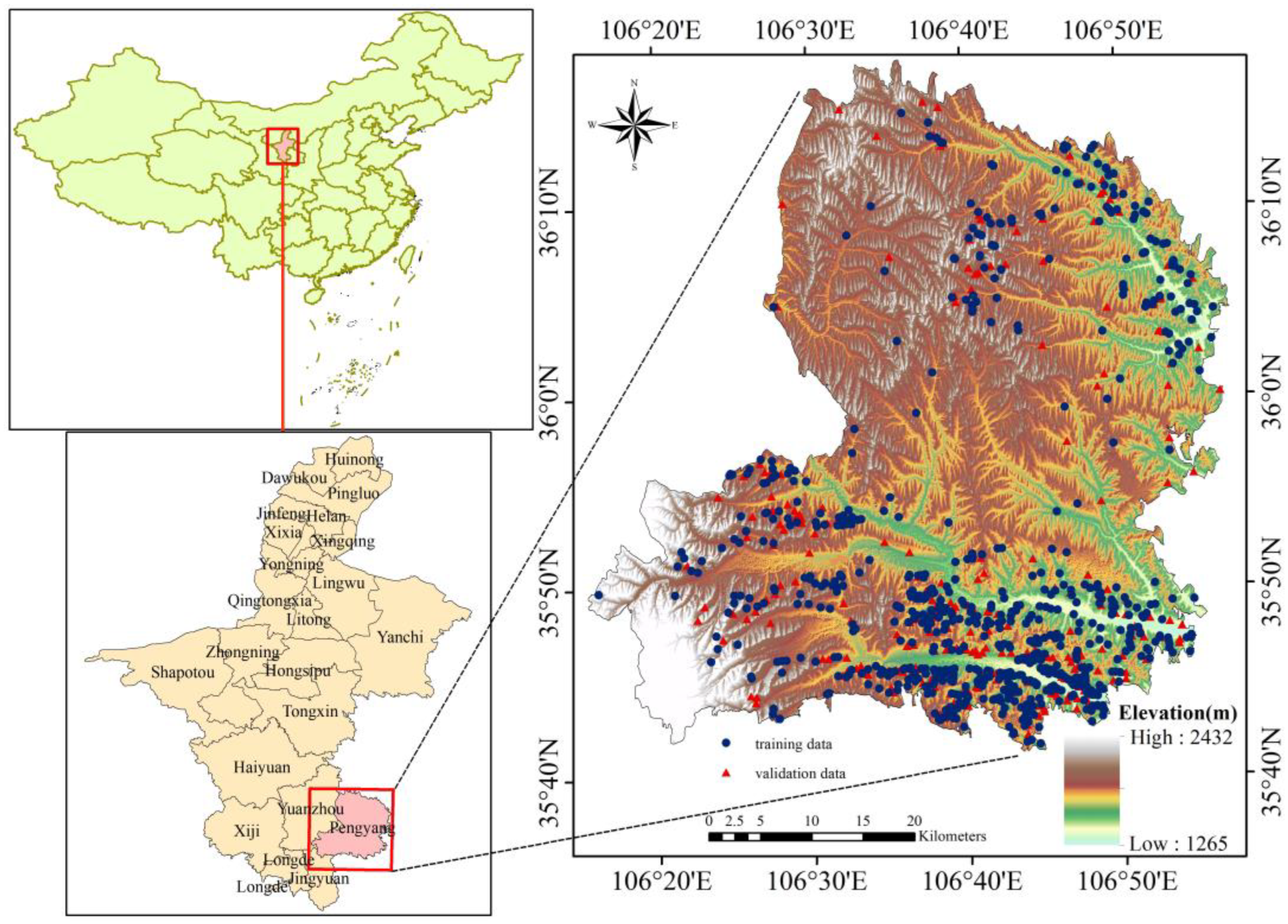
2.1. Geographic Location

Pengyang County is situated in the southeastern edge of Ningxia at the eastern foot of Liupan Mountain. It falls under the administrative jurisdiction of Guyuan City and shares its borders with Zhenyuan County, Pingliang City, and Huan County of Gansu Province to the east, south, and north, respectively. To the west, it is adjacent to the Yuanzhou District of Ningxia. The county is geographically located from 106°32′ to 106°58′ east longitude and 35°41′ to 36°17′ north latitude, encompassing a total area of 2533.49 km². It spans approximately 62 km from north to south and approximately 58 km from east to west (Figure 1).

2.2. Climate

Pengyang County experiences a temperate semi-humid and semi-dry climate, marked by four distinct seasons. It has hot and rainy summers, while winters tend to be dry with less rainfall. The average annual temperature is 6.3 °C, with the highest temperatures typically occurring in July, averaging around 19.0 °C; the lowest temperatures occur in January, averaging approximately −8.2 °C. Precipitation levels in most areas of the region range from 400 to 500 mm, gradually decreasing from south to north, resulting in a difference of approximately 150 mm between the two ends. The annual precipitation in Pengyang County displays significant interannual variability. Within the same year, the distribution of precipitation is highly uneven, characterized by distinct rainy and dry seasons. Rainfall mainly occurs in the form of continuous overcast and rainy days, as well as heavy rain events.

2.3. Topography

Slope topography is a fundamental factor contributing to landslides. In Pengyang County, the thickness of loess accumulation varies from tens of meters to over 100 m, which is characterized by a loose structure, significant rock and soil erosion, and the presence of well-developed surface water systems [49]. The region features numerous river tributaries and a rugged topography, creating favorable topographic and geomorphologic conditions conducive to the occurrence of landslides. The landforms in Pengyang County mainly consist of loess hilly area, stony mountainous terrain, and a valley district, which account for 86.68%, 7.94%, and 5.38% of the total area, respectively (Figure 2).

2.4. River System

The rivers within Pengyang County are part of the Jing River system, which is primarily composed of the Ru River, Hong River, Anjiachuan River, and various smaller streams (Figure 3). The Ru River and Hong River flow in an east-to-west direction, encompassing a sizable watershed area. In Yuanzhou District, water resources are limited, and there is a notable contrast in water quality, with poorer quality water being found in the northern part of the district and better quality water being found in the southern region. Atmospheric precipitation serves as the primary source of surface water within the district [50].

Given the uneven distribution of annual precipitation and occasional heavy rainfall in Pengyang County, there is a significant issue with rock and soil erosion. The rugged terrain further exacerbates these conditions, creating natural predispositions for landslide development. Consequently, Pengyang County experiences a high number of landslides that are widely distributed throughout the region. This underscores the necessity of studying landslide susceptibility in this area.

3. Methodology

This study can be divided into four stages (Figure 4): (1) the construction of the landslide inventory map and preparation of the landslide conditioning factors; (2) an analysis of the correlation between landslides and conditioning factors; (3) an evaluation of landslide susceptibility using LR, FT, and RSFT models; and (4) a comparison of the accuracy of the three models and the selection of the optimal model.

3.1. Preparation of Spatial Database

The landslide allocation map was generated using historical landslide records, field investigations (part of the Geological Hazard Detailed Investigation Project at a 1:50,000 scale in Pengyang County), and interpretation of satellite images (GF-2). Unlike previous studies that have often represented landslides as individual points for analyzing their spatial distribution, this study took a different approach. We compiled a comprehensive dataset consisting of 972 landslide locations within the study area. Out of this dataset, a total of 680 landslide locations were meticulously selected for the training dataset, while the remaining 292 locations formed the verification dataset. This careful selection process ensured the effective utilization of both datasets for the study (refer to Figure 1 for further details). To ensure a balanced representation, an equal number of non-landslide-prone areas were randomly chosen from regions prone to landslides. These non-landslide-prone areas were then split into two separate groups, maintaining a 70:30 ratio. This division facilitated the creation of both the training and validation datasets, respectively. This methodology ensured a robust and unbiased evaluation of the models’ performance. The division guaranteed that both datasets contained representative samples of non-landslide-prone areas, allowing for the effective training and validation of the landslide susceptibility analysis models [46,51,52,53,54,55,56,57]. The landslide inventory map and survey data analysis revealed that the primary type of landslides in the study area were tractive landslides (Figure 5), which mainly occurred along river and valley slopes (Figure 1). Due to the varying sizes of landslides, the statistical calculations in this study were based on the area of landslides without categorizing them in multiple ways by type or characteristics. It is important to note that all data utilized in this research were generously provided by the Ningxia Land Resources Survey and Monitoring Institute.

Various factors play a significant role in influencing the occurrence of landslide-prone areas, which are collectively known as landslide conditioning factors. [20,58,59,60]. In this study, we conducted extensive research on the local geological environment and characteristics of landslide development. Moreover, we analyzed the relationship between the occurrence of landslides and the conditions in the study area in collaboration with previous scholars, leading to the identification of 15 conditioning factors [50]. These factors include the slope angle, elevation, profile curvature, plan curvature, slope aspect, topographic wetness index (TWI), topographic position index (TPI), distance from roads, distance from rivers, normalized difference vegetation index (NDVI), rainfall, land use, lithology, stream power index (SPI), and sediment transport index (STI). The thematic map resolution for each conditioning factor is set at 25 × 25 m.

Among the array of factors examined, slope angle emerges as a pivotal element significantly influencing slope instability. It is widely recognized as a critical factor and is commonly integrated into landslide susceptibility models [61,62]. In this study, the slope angle was categorized into one grade for every 10 degrees in the range of 0–60 degrees, with an additional grade for slopes greater than 60 degrees, resulting in a total of 7 grades. (Figure 6a).

Elevation holds substantial importance in landslide susceptibility analysis due to its pivotal role in determining the stress distribution of a slope [63,64,65]. For this study, the elevation map was derived from digital elevation model (DEM) datasets with 200 m intervals. Seven elevation categories were established: <1300 m, 1300–1500 m, 1500–1700 m, 1700–1900 m, 1900–2100 m, 2100–2300 m, and >2300 m (Figure 6b).

Profile curvature is a metric used to quantify variations in ground elevation along the maximum slope direction of a terrain surface, which in turn influences airflow acceleration across the surface [66,67,68,69,70]. The profile curvature value is derived from a digital elevation model (DEM) and directly reflects the geometric characteristics of the slope profile. In this research, section curvature was categorized into ranges of 11.54 to 9.14, 11.54 to 1.08, 1.08 to 0.43, 0.43 to 0.22, 0.22 to 0.95, and 0.95 to 9.145 (Figure 6c).

Plane curvature, on the other hand, results from the slope aspect analysis of the DEM and significantly impacts surface runoff and infiltration characteristics [71,72,73,74,75,76,77]. The range of plane curvature in this study spanned from −5.63 to 7.68 and was divided into five categories: −5.3 to −0.98, −0.98 to 0.37, −0.37 to 0.25, 0.25 to 0.91, and 0.91 to 7.68 (Figure 6d).

Slope aspect refers to the orientation or direction of the slope’s free surface, which is a crucial factor in evaluating landslide sensitivity [78,79]. It can affect slope stability through variations in precipitation, wind, solar radiation, climate conditions, vegetation, soil, geomorphology, hydrology, and more [80,81,82,83]. For instance, this study found that slopes facing north are generally more prone to landslides than those facing south. The slope direction map was generated using DEM data and was divided into 10 categories (Figure 6e).

The topographic wetness index (TWI) plays a significant role in landslide analysis and is calculated as TWI = ln(a/tanβ) [78,81,82], combining the local uphill contribution area (a), representing water flow towards a specific location, with the local slope (tanβ). The resulting TWI map was classified into five distinct classes: 2.21–6, 6–10, 10–14, 14–18, and >−18, as shown in Figure 6f.

The terrain position index (TPI) measures the slope position of the terrain and automatically classifies it [84]. TPI values in this study ranged from −34.64 to 37.93 and were divided into five categories using the Jenks natural fracture classification method (Figure 6g).

Human engineering activities, particularly road construction, have a significant impact on the geological environment and can influence the occurrence of landslides [85]. The proximity between a slope and a road is considered a conditioning factor, with six buffer zones being constructed at intervals of 100 m, ranging from 0–100 m to >500 m (Figure 6h).

Figure 3 depicts the water system map of the study area, and the seepage erosion of these rivers at the foot of slopes can alter the slope’s nature and significantly impact landslides [86,87,88,89]. Consequently, the distance between the slope and the river was also considered a conditioning factor, and it was divided into six categories ranging from 0–200 m to >1000 m. (Figure 6i).

The normalized difference vegetation index (NDVI) holds significant importance in the assessment of landslide susceptibility and is commonly used in related studies due to its ability to indicate vegetation growth levels and their correlation with surface infiltration, runoff, and weathering dynamics [90,91]. In this study, NDVI values were computed and subsequently categorized into five distinct levels, ranging from −0.22 to 0.03, 0.03 to 0.11, 0.11 to 0.15, 0.15 to 0.19, and 0.19 to 0.43 (Figure 6j).

Rainfall is a significant factor in triggering landslides [92,93,94,95], particularly in the study area, where rainfall-induced landslides are prevalent. Rainfall distribution gradually increases from north to south, with the southern region experiencing a higher concentration of landslides. Therefore, rainfall is recognized as a crucial factor influencing landslide occurrence in the study area. To analyze its impact, a rainfall factor map was generated based on the annual mean rainfall map. The rainfall factor map categorized rainfall levels into five intervals at 20 mm/year increments: <450 mm/year, 450–470 mm/year, 470–510 mm/year, 510–530 mm/year, and >530 mm/year (Figure 6k).

Land use type represents another significant factor influencing landslide susceptibility [96,97,98]. In this study, land use types were classified into five categories: agricultural land, forest, grassland, water, and residential areas (Figure 6l).

Different physical and mechanical properties of soils and rocks are key factors affecting slope stability [99,100]. In this study, nine lithology types were identified using a geological map at a scale of 1:50,000 (Figure 6m).

The stream power index (SPI) is a factor related to rock lithology, grain size, and permeability; it is used to measure the frequency of surface water erosion and sediment transport on the landscape [101,102]. Fine channel erosion and sediment accumulation can often occur on the slope surface, and instability may occur when the slope shear stress exceeds the surface shear strength. The SPI in this study was divided into five classes ranging from 0–200 to >800 (Figure 6n).

The Sediment Transport Index (STI) is utilized to quantify the sediment transport capacity of an area [103,104]. Generally, areas with high runoff volumes have a greater ability to transport sediment compared with areas with lower runoff volumes. In this study, the STI was classified into five classes using the natural interval method. The classification ranges were as follows: 0–1.89, 1.89–4.12, 4.12–6.36, 6.36–9.11, and 9.11–42.8, respectively (Figure 6o).

3.2. Spatial Prediction Modeling of Landslides

3.2.1. Certainty Factor (CF)

Researchers commonly employ the certainty factor (CF) model in the field of landslide susceptibility mapping [105,106]. The CF method provides a valuable approach for addressing the challenge of integrating diverse data layers while considering the heterogeneity and uncertainty of the input data. To determine the CF, an equation can be used as follows (Equation (1)):

$$\mathrm{C}\mathrm{F}=\left\{\begin{array}{c}\frac{\mathrm{P}\mathrm{P}\mathrm{a}-\mathrm{P}\mathrm{P}\mathrm{s}}{\mathrm{P}\mathrm{P}\mathrm{a}(1-\mathrm{P}\mathrm{P}\mathrm{s})} \mathrm{i}\mathrm{f} \mathrm{P}\mathrm{P}\mathrm{a}\ge \mathrm{P}\mathrm{P}\mathrm{s}\\ \frac{\mathrm{P}\mathrm{P}\mathrm{a}-\mathrm{P}\mathrm{P}\mathrm{s}}{\mathrm{P}\mathrm{P}\mathrm{s}(1-\mathrm{P}\mathrm{P}\mathrm{s})} \mathrm{i}\mathrm{f} \mathrm{P}\mathrm{P}\mathrm{a}\le \mathrm{P}\mathrm{P}\mathrm{s}\end{array}\right.$$

(1)

In this equation, PPa represents the conditional probability of an event occurrence within the impact factor hierarchy. It is determined by the ratio of the number of grids where landslides occurred to the total number of grids within each factor. On the other hand, the prior probability (PPs) indicates the likelihood of landslide occurrence across the entire study area. It is determined by dividing the number of grids with landslides by the total number of grids in the study area.

The condition factor (CF) is a numerical measure that falls within the range of −1 to 1. A CF value close to 1 signifies a strong positive correlation between the variables being assessed. In this context, it suggests a robust positive relationship between the condition factor and landslide incidence.

3.2.2. Logistic Regression (LR)

The logistic regression (LR) model is employed to evaluate the occurrence of landslides as a binary problem, and it determines whether a landslide occurs or not. It allows for the assessment of the impact of various factors and parameters on landslide occurrence and the prediction of landslide probability [80,88].

The generalized linear model (GLM) is a statistical model that incorporates logistic regression and enables the establishment of multiple regression relationships between dependent and independent variables [107,108]. In landslide susceptibility assessment, the LR model aims to identify the optimal model that describes the relationship between the presence (dependent variable) and absence (binary values 0 and 1) of landslides. It accomplishes this by considering a set of causal factors, also known as independent variables [31]. A binary logistic regression model is then developed to identify the optimal fitting model [109,110]. The binary logistic regression model is expressed mathematically as follows (Equation (2)):

$$\mathrm{P}=\frac{1}{1+{\mathrm{e}}^{-\mathrm{z}}}$$

(2)

Here, P represents the probability of landslide occurrence, ranging from 0 to 1, and z is the linear combination of a constant, an independent variable, and its coefficient. It can be represented as (Equation (3)):

$$\mathrm{z}={\mathsf{\beta }}_0+{\mathsf{\beta }}_1{\mathrm{x}}_1+{\mathsf{\beta }}_2{\mathrm{x}}_2+\cdots +{\mathsf{\beta }}_{\mathrm{n}}{\mathrm{x}}_{\mathrm{n}}$$

(3)

Among them, ${\mathsf{\beta }}_0,{\mathsf{\beta }}_1,{\mathsf{\beta }}_2,\cdots ,{\mathsf{\beta }}_{\mathrm{n}}$ are the parameters of the model, while ${\mathrm{x}}_1,{\mathrm{x}}_2,\cdots ,{\mathrm{x}}_{\mathrm{n}}$ are the independent variables, which are factors related to the occurrence of landslides. In the LR model, the model parameters need to be estimated, and the commonly used method is maximum likelihood estimation. This involves finding the parameter values that maximize the probability of the dependent variable given the independent variables. Ultimately, the resulting model can be used to predict whether landslides will occur at new data points, providing important support for landslide prevention and control [86,111,112].

3.2.3. Functional Trees (FTs)

The Functional Tree (FT) model is a powerful tool for processing large-scale data. Its core idea is to divide the dataset into multiple subsets, aggregate and process each subset, and finally merge the results into a complete result set. This process can be carried out recursively until the final result is achieved. In the FT model, each node is a function that receives input data and returns processing results. Each node has multiple children, and each child node corresponds to a subset of the data. When a node is called, it assigns input data to its children and waits for their processing results. When all child nodes return results, the node aggregates the results of all child nodes and returns them to its parent node. The FT model is typically structured as a tree, with the root node representing the entire dataset and each leaf node corresponding to one data item. In this model, each node is a pure function that only depends on its input parameters and does not modify external state, making it well-suited for parallelization [113].

Consider a training dataset D consisting of n samples $(X_i,Y_i)$ where $X_i\in {\mathrm{R}}^{\mathrm{n}}$ represents an input vector comprising the 15 landslide conditioning factors mentioned earlier and where $Y_i\in \left\{\mathrm{1,0}\right\}$ represents the output variable and consists of two classes: landslide and no-landslide. Functional Trees (FTs) aim to create a decision tree that accurately distinguishes between the two classes using the given training data. The key difference between traditional decision tree algorithms and FTs lies in the splitting process at the tree nodes. While traditional algorithms utilize a constant value to compare input attribute values and partition the data, FTs utilize logistic regression functions for oblique splits at inner nodes and make predictions at the leaves. This oblique splitting approach allows FTs to capture more complex relationships and interactions between the input variables, enhancing their ability to accurately classify the data into the landslide and no-landslide classes [114,115,116,117].

The FT algorithm incorporates several techniques to enhance its performance: (1) splitting criterion: the gain ratio is utilized as the criterion for selecting the input attribute to split on at each tree node; (2) pruning: to prevent overfitting and improve generalization, standard C 4.5 pruning is applied to the constructed decision tree; and (3) logistic regression at leaves: at the leaves of the decision tree, logistic regression functions are fitted using the LogitBoost algorithm. The least-squares fits are employed for each class $Y_i$ (Equation (4))

$$f_{Y_i}\left(X\right)={\sum }_{i=1}^{15}{\mathsf{\beta }}_i{X}_i+{\mathsf{\beta }}_0$$

(4)

where $\mathrm{P}\left(X\right)$ represents the predicted probability value, ${\mathsf{\beta }}_i$ denotes the coefficient of the ith component in the input vector $X_i$, and N is the number of components. The posterior probabilities in the leaves, $\mathrm{P}\left(X\right)$, are calculated accordingly (Equation (5)):

$$\mathrm{P}(X)=\frac{{\mathrm{e}}^{2f_{Y_i}\left(X\right)}}{1+{\mathrm{e}}^{2Y_i\left(X\right)}}$$

(5)

3.2.4. Random Subspace Functional Trees (RSFTs)

Random subspace (RS) is an integrated learning technique introduced by Ho, also known as attribute bagging or feature bagging. This stochastic subspace model combines two algorithms. Firstly, the proposed method generates low-dimensional subspaces by randomly sampling high-dimensional feature vectors. Within these subspaces, multiple classifiers are combined to generate prediction results. [118,119,120]. In other words, the RS model differs from other methods by randomly selecting features from the original training dataset. Compared with traditional methods such as bagging, boosting, and rotation forest, RS has been shown to be superior [118].

Currently, RS has found widespread applications in fields such as automation technology [121], computer software, computer applications [122], telecommunication technology [123], mathematics [124], and many others. However, it has been rarely used in research fields related to geology, especially in the context of landslide susceptibility research.

Let us consider a training dataset, denoted as $Z={(Z}_1,Z_2,\dots ,Z_i)$,$\left(i=\mathrm{1,2},\dots ,\mathrm{n}\right)$, where Zᵢ is a p-dimensional vector and i ranges from 1 to n. In the random subspace (RS) method, an r-dimensional vector $\widehat{Z}$_i is derived from the p-dimensional vector $Z$_i (r < p). where r < p. The r-dimensional random subspace can be represented as (Equation (6)):

$$\widehat{Z}=\left[\begin{array}{cccc}{\widehat{Z}}_{11}& {\widehat{Z}}_{21}& \dots & {\widehat{Z}}_{n1}\\ {\widehat{Z}}_{12}& {\widehat{Z}}_{22}& \dots & {\widehat{Z}}_{n2}\\ \dots & \dots & \dots & \dots \\ {\widehat{Z}}_{1r}& {\widehat{Z}}_{2r}& \dots & {\widehat{Z}}_{nr}\end{array}\right]$$

(6)

To obtain multiple random subspaces, this selection process is repeated several times. Each subspace $\widehat{Z}$ is used to construct a classifier C(x), and the results of these classifiers are combined using a simple majority vote [125]. The final decision rule is defined as follows (Equation (7)):

$$\beta \left(x\right)=\arg \max {\sum }_b^{\delta }{\delta }_{\mathrm{s}\mathrm{g}\mathrm{n}}\left(c^b\left(x\right)\right),y;y\in \left\{-\mathrm{1,1}\right\}$$

(7)

where ${\mathsf{\delta }}_{i,j}(\mathrm{i}=\mathrm{1,2},\dots ,n,j=\mathrm{1,2},\dots ,r)$ represents the Kronecker symbol and $\mathrm{y}\in \left\{1,-1\right\}$ is a class label indicating landslide or non-landslide.

The RSFT model, as mentioned in Section 3.2.3, is a combination of two models: random subspace (RS) and functional trees (FTs). It involves the following steps: (1) Randomly select the feature subspace: In this step, a smaller subset of features is randomly chosen from the original feature set. This selection can be achieved through methods such as random selection or feature importance evaluation. (2) Construct the function tree: The selected feature subspace is used to construct a function tree. At each node of the tree, the best segmentation function is chosen to divide the data into different subsets. The segmentation function can be linear, non-linear, or of other types. The construction of the tree is performed recursively until a predefined stopping condition is met, such as reaching the maximum tree depth or having a sample count below a certain threshold. (3) Repeat the first two steps: These steps are repeated multiple times, with each iteration utilizing a different feature subspace and a randomly selected feature subset. This process results in the construction of multiple function trees, each with a unique set of features. (4) Prediction: The final prediction category is determined by aggregating the predictions of multiple function trees. This can be achieved through voting, where each tree’s prediction contributes to the final decision. By combining the RS and FT models, RSFT aims to leverage the benefits of both approaches. The RS component introduces randomness by considering different feature subspaces, while the FT component incorporates the use of function trees for improved modeling and prediction. This hybrid approach helps reduce repetition and enhances the overall performance of the model.

4. Results

4.1. Correlation between Landslides and Conditioning Factors

The relationship between the landslide location and adjustment factor is shown in

Table 1. Spatial relationship between landslides and conditioning factors using the CF method.

Conditioning Factors	Class	Pixels	Landslides Pixels	$\mathbf{P}\mathbf{P}\mathbf{a}$	CF
Slope angle (°)	0–10	1,233,976	9539	0.0077	−0.472
	10–20	1,884,829	31,370	0.0166	0.128
	20–30	808,346	16,669	0.0206	0.299
	30–40	121,503	1454	0.0120	−0.180
	40–50	6305	0	0.0000	−0.98
	50–60	221	0	0.0000	−1
	>60	8	0	0.0000	−1
Elevation (m)	<1300	6481	1	0.0002	−0.985
	1300–1500	666,680	16,643	0.0250	0.423
	1500–1700	2,225,730	33,370	0.0150	0.030
	1700–1900	977,391	8945	0.0092	−0.374
	1900–2100	121,612	73	0.0006	−0.959
	2100–2300	46,744	0	0.0000	−1
	>2300	11,320	0	0.0000	−1
Profile curvature	−11.54–−1.08	197,001	1592	0.0081	−0.448
	−1.08–−0.43	913,652	10,276	0.0112	−0.230
	−0.43–0.22	1,587,299	30,351	0.0191	0.243
	0.22–0.95	1,085,198	13,861	0.0128	−0.124
	0.95–9.14	272,807	2951	0.0108	−0.259
Plan curvature	−5.3–−0.98	194,476	2913	0.0150	0.029
	−0.98–−0.37	896,797	15,324	0.0171	0.151
	−0.37–0.25	1,684,370	24,543	0.0146	0.001
	0.25–0.91	1,041,768	11,731	0.0113	−0.229
	0.91–7.68	238,546	4520	0.0189	0.236
Slope aspect	F	28,771	0	0.0000	−1
	N	214,182	2853	0.0133	0.214
	NE	582,880	6117	0.0105	−0.282
	E	729,709	5268	0.0072	−0.508
	SE	420,997	2582	0.0061	−0.582
	S	387,178	8034	0.0208	0.303
	SW	467,527	6471	0.0138	−0.49
	W	618,183	12,621	0.0204	0.292
	NW	455,474	9785	0.0215	0.327
	N	150,287	5301	0.0353	0.596
TWI	2.21–6	2,328,468	35,112	0.0151	0.036
	6–10	1,451,293	21,950	0.0151	0.039
	10–14	201,447	1709	0.0085	−0.420
	14–18	55,808	129	0.0023	−0.842
	>18	18,942	131	0.0069	−0.529
TPI	−34.64–−7.04	324,193	4526	0.0140	−0.041
	−7.04–−2.2	899,770	10,850	0.0121	−0.173
	−2.2–1.78	1,438,547	21,517	0.0150	0.028
	1.78–6.34	997,182	14,002	0.0140	−0.035
	6.34–37.93	396,266	8137	0.0205	0.296
Distance to roads (m)	0–100	232,634	2893	0.0124	−0.147
	100–200	207,063	10,041	0.0485	0.710
	200–300	195,015	13,289	0.0681	0.798
	300–400	189,552	10,407	0.0549	0.746
	400–500	179,935	5074	0.0282	0.491
Distance to rivers (m)	0–200	899,311	4349	0.0048	−0.671
	200–400	767,341	4570	0.0060	−0.594
	400–600	600,724	4300	0.0072	−0.512
	600–800	426,497	4860	0.0114	−0.219
	800–1000	271,523	4276	0.0157	0.077
	>1000	1,078,500	36,676	0.0340	0.581
NDVI	<0.03	6732	0	0.0000	−1
	0.03–0.11	573,462	5068	0.0088	−0.396
	0.11–0.15	2,027,374	26,021	0.0128	−0.119
	0.15–0.19	1,180,464	23,438	0.0199	0.271
	0.19–0.43	255,862	4506	0.0176	0.176
Rainfall (mm/yr)	<450	3007	0	0.0000	−1
	450–470	718,693	724	0.0010	−0.932
	470–490	1,544,756	8802	0.0057	−0.612
	490–510	1,714,702	46,595	0.0272	0.471
	>510	62,471	2911	0.0466	0.698
Land use	farmland	1,675,029	29,433	0.0176	0.175
	forest	215,769	1698	0.0079	−0.463
	grass	2,114,613	27,901	0.0132	−0.094
	water	18,869	0	0.0000	−1
	residentialareas	20,311	0	0.0000	−1
Lithology	1	223,561	2	0.0000	−0.999
	2	3,387,689	54,833	0.0162	0.103
	3	1804	10	0.0053	−0.638
	4	1889	0	0.0000	−1
	5	70,175	1157	0.0165	0.199
	6	26,678	833	0.0312	0.542
	7	326,333	1757	0.0054	−0.633
	8	548	440	0.8028	0.996
	9	81	0	0.0000	−1
SPI	0–200	748,095	3344	0.0045	−0.696
	200–400	1,239,924	25,522	0.0206	0.297
	400–600	1,151,603	17,331	0.0150	0.034
	600–800	591,663	8632	0.0146	0.003
	>800	324,673	4202	0.0129	−0.126
STI	0–1.89	964,332	7705	0.0080	−0.833
	1.89–4.12	1,275,764	20,177	0.0158	0.088
	4.12–6.36	1,018,068	17,450	0.0171	0.181
	6.36–9.11	597,977	11,886	0.0199	0.374
	9.11–42.8	199,817	1813	0.0091	−0.613

using the CF (certainty factor) method.

According to Table 1, it is evident that slope angle classes of 20–30° (0.299) and 10–20° (0.128) exhibit the highest number of landslides, indicating a significantly higher probability of landslide occurrence within these ranges. Conversely, the CF values for other slope angle ranges are less than 0, indicating a very low probability of landslide occurrence in those intervals. Regarding elevation, the CF value is above 0 in the range of 1300–1500 m, suggesting a higher probability of landslide occurrence at this elevation. However, the CF value decreases as elevation increases, indicating a decreasing likelihood of landslides at higher elevations. In terms of profile curvature, the range of −0.432 to 0.22 exhibits the highest probability of slope damage, as indicated by a CF value of 0.243. In contrast, the CF values associated with different intervals of profile curvature are predominantly negative, suggesting a reduced likelihood of landslide occurrence.

For plan curvature, the highest probability of landslide occurrence lies within the 0.91–7.68 category with a maximum CF value of 0.236. The observed pattern indicates that as the plan shape transitions from concave to convex, the stability of the slope tends to improve.

Overall, these findings provide valuable insights into the relationships between various factors and the probability of landslide occurrence. They highlight the importance of slope angle, elevation, profile curvature, and plan curvature in assessing landslide susceptibility and can aid in implementing appropriate mitigation measures. Regarding slope aspect analysis, most landslides occur towards the north (0.596) and northwest (0.327), while the CF values are less than 0 for slopes facing east and southeast, southwest, and northeast. In terms of soil moisture, the ranges of 6–10 and 2.21–6 have the highest susceptibility to slope damage, with CF values of 0.039 and 0.036, respectively, while the CF values for the other ranges are less than 0. This indicates that soil moisture has a greater influence on landslide development. Regarding the distance from the road, the CF values for the ranges of 100–300 m and 300–400 m are all above 0.7, indicating a high probability of slope damage within these distances. As the distance from the road increases, the likelihood of slope damage decreases. Conversely, in terms of distance from rivers, the CF value increases as the distance decreases, suggesting a higher probability of slope damage with closer proximity to a river. The highest CF value is 0.581 in the >1000 m category, indicating that landslides mainly occur on slopes in loess hilly areas far from rivers. The NDVI analysis indicates that the sensitivity of landslide occurrence is elevated in the range of 0.15–0.19 (CF value of 0.271) and 0.19–0.43 (CF value of 0.176). These ranges suggest a higher likelihood of landslides in areas with these specific NDVI values. Regarding the influence of rainfall on landslides, the results demonstrate that a significant proportion of landslides in the study area are induced by rainfall. Moreover, the probability of landslides occurring increases as the amount of rainfall increases [126]. In terms of land use type, the highest CF value was found for cropland (0.175), followed by grassland (−0.094) and finally forest land (−0.463). With respect to the lithology, the CF value of the eighth group (shale) is the highest at 0.996, but due to the limited number of shale samples, the error is relatively large and this finding is therefore not discussed. The CF value of the sixth group (sandstone and sandy mudstone) is 0.542, while the CF values of the fifth group (Brown-red mudstone) (0.199) and second group (loess) are relatively high, indicating a higher probability of slope failure for these lithological units. Finally, the analysis results of SPI show that the CF value is lowest in the range of 0–200 (−0.696) and highest in the range of 200–400 (0.297). Regarding STI, the CF value is lowest in the ranges of 0–1.89 (−0.833), while the highest CF value is in the range of 6.36–9.11 (0.374).

4.2. Multicollinearity Analysis of Landslide Conditioning Factors

Multicollinearity in landslide studies refers to the high correlation and non-independence of conditioning factors in datasets, which can lead to inaccurate system analysis. To quantify multicollinearity, various methods are available, including variance decomposition proportions, the conditional index, and the widely used variance inflation factors (VIFs) and tolerances. VIFs and tolerances methods are frequently employed to assess multicollinearity among conditioning factors in landslide studies.

A multicollinearity analysis was conducted using SPSS 27.0.1 software, and the correlation between the 15 conditioning factors is presented in

Table 2. Multicollinearity analysis for the landslide conditioning factors.

NO.	Factor	TOL	VIF
1	Slope angle	0.681	1.469
2	Elevation	0.836	1.196
3	Profile curvature	0.970	1.031
4	Plan curvature	0.981	1.020
5	Slope aspect	0.958	1.044
6	TWI	0.785	1.274
7	TPI	0.944	1.060
8	Distance to roads	0.759	1.317
9	Distance to rivers	0.680	1.470
10	NDVI	0.931	1.074
11	Rainfall	0.855	1.169
12	Landuse	0.943	1.060
13	Lithology	0.799	1.251
15	STI	0.586	1.705

. In general, the presence of covariance in the data can be indicated when the tolerance (TOL) is below 0.1 or the variance inflation factor (VIF) is above 10. Conversely, values within these ranges suggest no significant covariance. The analysis results indicate that there is no evidence of collinearity among the factors. Therefore, all of these conditioning factors can be considered suitable inputs for the machine learning algorithm.

4.3. Contribution of Conditioning Factors

To assess the contribution of landslide conditioning factors, a comparative analysis was conducted utilizing the CorrelationAttributeEval function available in Weka 3.9 software. The results, presented in

Table 3. Assessing the relevance of conditioning factors using CorrelationAttributeEval.

NO.	Factors	Relevance
1	Rainfall	0.3534
2	Distance to rivers	0.3287
3	Elevation	0.2899
4	Lithology	0.26
5	Slope angle	0.2347
6	SPI	0.1856
7	Slope aspect	0.112
8	Distance to roads	0.0908
9	NDVI	0.0884
10	TPI	0.0525
11	Plan curvature	0.0483
12	STI	0.0448
13	TWI	0.0435
14	Land use	0.0264
15	Profile curvature	0.0188

and Figure 7, indicate that all factors play a role in the model. Notably, rainfall emerges as the most important factor, with a correlation value of 0.3534. This is followed by the distance to rivers (0.3287) and elevation (0.2899) as significant contributors. Conversely, factors such as TWI (0.0435), land use (0.0264), and profile curvature (0.0188) have relatively smaller contributions to the landslide model. Given that all 15 conditioning factors exhibited positive contributions in the analysis, it was determined that all of them would be taken into account during the construction of landslide susceptibility maps. By considering all conditioning factors, a comprehensive and robust understanding of the factors contributing to landslide susceptibility can be achieved, leading to more accurate and reliable susceptibility maps.

4.4. Application of LR Model

In this study, the LR (Logistic Regression) model was implemented using Weka 3.9 statistical software to generate the landslide susceptibility mapping. To evaluate the model’s accuracy, the mean squared error (MSE) was computed for both the training and validation datasets. The MSE values obtained were 0.177 for the training data and 0.176 for the validation data (Figure 8b). To facilitate the creation of the landslide susceptibility map, all LSI (latent semantic indexing) values were converted into ArcGIS format. This conversion allowed for seamless integration with ArcGIS 10.8 software, enabling efficient mapping and analysis. The resulting landslide susceptibility map was classified into five classes using the natural break method. The classified map obtained through this process is presented in Figure 9. The reclassified results are presented in

Table 4. Statistics table of the five susceptibility levels in the susceptibility maps of the three models.

Model Type	Levels	Reclassified Value	Area Covered (%)
LR model	Very Low	0–0.145	26.98
	Low	0.145–0.306	24.02
	Moderate	0.306–0.486	19.65
	High	0.486–0.678	16.22
	Very High	0.678–1	13.13
	Total	0–1	100
FT model	Very Low	0–0.161	76.92
	Low	0.161–0.478	1.51
	Moderate	0.478–0.717	3.97
	High	0.717–0.894	7.26
	Very High	0.894–1	10.34
	Total	0–1	100
RSFT model	Very Low	0–0.147	34.72
	Low	0.417–0.311	25.42
	Moderate	0.311–0.512	17.67
	High	0.512–0.734	14.22
	Very High	0.734–0.990	7.97
	Total	0–0.990	100

and Figure 10. Among the susceptibility categories, the “very low susceptible” category exhibited the largest area percentage, accounting for 26.98% of the total area. The area percentages of the “low”, “medium”, “high”, and “extremely susceptible” categories were 24.02%, 19.65%, 16.22%, and 13.12%, respectively.

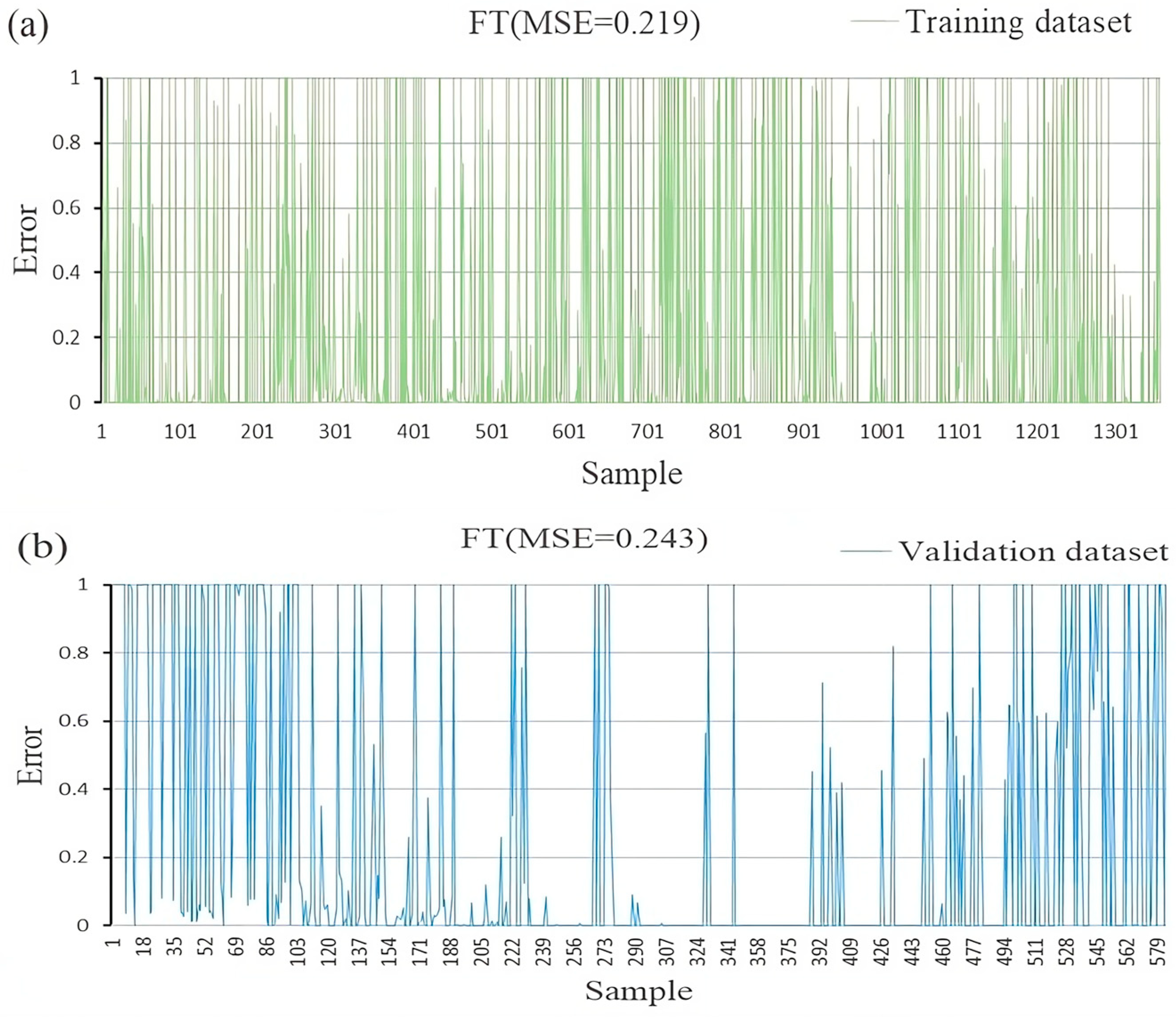
4.5. Application of FT Model

For constructing the FT model, this research utilized Weka 3.9 software, which incorporated all fifteen conditioning factors. For model evaluation, mean squared error (MSE) values were computed for both the training and validation datasets. These MSE values are depicted in Figure 11a for the training dataset and Figure 11b for the validation dataset, respectively. The computed MSE values were 0.219 for the training data and 0.243 for the validation dataset. Following this, all datasets were fed into the FT model to generate landslide susceptibility index values, representing probabilities ranging from 0 to 1. Finally, ArcGIS 10.2 software was utilized to produce the final landslide susceptibility map.

Landslide susceptibility classification methods can be categorized as either user-defined or automatic. The user-defined method is subjective and prone to variations in the final results due to individual opinions. In contrast, the natural break method utilizes digital elevation models and other geographic data to extract information, leading to more accurate data and reducing the potential for human error. In this study, an automatic classification system known as the natural break method was utilized to subdivide the landslide susceptibility. This method helps to categorize the susceptibility values into distinct groups based on natural breaks in the data distribution. Based on the analysis, the landslide susceptibility map was divided into five distinct classes: very low, low, moderate, high, and very high susceptibility. The reclassification results are presented in Figure 9, Table 4, and Figure 10, providing additional insights into the distribution of these susceptibility classes. Notably, the largest percentage of the study area corresponds to the very low susceptibility class, encompassing approximately 76.92% of the total area. Following that, the very high susceptibility class represents around 10.34% of the area, while the high susceptibility class covers approximately 7.26%. The moderate susceptibility class accounts for approximately 3.97% of the area, and the low susceptibility class encompasses roughly 1.51% of the study area.

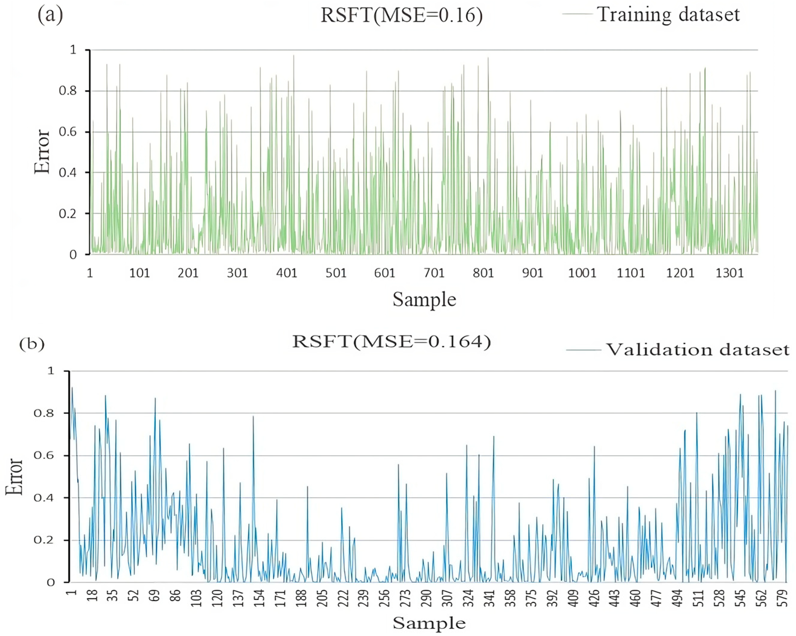
4.6. Application of RSFT Model

In this study, the RSFT model was implemented using Weka 3.9 software. The predictive power of the RSFT model was evaluated by incorporating the training and validation datasets and by calculating the mean squared error (MSE) values for each dataset. The MSE values that were obtained were 0.16 for the training data (Figure 12a) and 0.164 for the validation dataset (Figure 12b). Following the analysis, the landslide susceptibility map was categorized into five distinct classes using the natural break method. These classes were defined as very low, low, moderate, high, and very high susceptibility. The resulting classification can be observed in Figure 9c. An analysis of Table 4 and Figure 10 indicates that the “very low susceptible” class occupies the largest area percentage (34.22%), followed by “low susceptible” (24.92%), “moderate susceptible” (17.17%), “high susceptible” (13.82%), and “very high susceptible” (9.75%).

4.7. Validation and Comparison of Different Models

Validating the results is a critical component of landslide susceptibility research to ensure the reliability and scientific significance of predictive models. In this study, we compared the performance of three prediction models using the receiver operating characteristic curve (ROC), with the area under the ROC curve (AUC) serving as a quantitative measure of model evaluation. Figure 13 and Figure 14 display the ROC curves for the three models, illustrating their performance on the training and validation datasets, respectively. The summarized results of the three models can be found in

Table 5. Area under the curve of the three models on the training dataset.

Test Variables	LR	FT	RSFT
ROC Curve Area	0.811	0.776	0.844
Standard Error	0.0116	0.0125	0.0105
95% Confidence Interval	0.789 To 0.832	0.752 To 0.797	0.823 To 0.863
p Value	<0.0001	<0.0001	<0.0001

and

Table 6. Area under the curve of three models on training dataset.

Test Variables	LR	FT	RSFT
ROC Curve Area	0.814	0.760	0.837
Standard Error	0.0180	0.0188	0.0163
95% Confidence Interval	0.780 To 0.845	0.723 To 0.794	0.804 To 0.866
p Value	<0.0001	<0.0001	<0.0001

. In the ROC curve, the diagonal line represents the subject’s discriminative power of 0. The further away from the diagonal line, the stronger the predictive power. When considering the training dataset, the RSFT model demonstrates the highest prediction rate (0.844), followed by the LR model (0.811) and the FT model (0.776). The standard errors for the LR, FT, and RSFT models are 0.0116, 0.0125, and 0.0105, respectively. Similarly, for the validation dataset, the RSFT model achieves the highest prediction rate (0.837), followed by the LR model (0.814) and the FT model (0.760). The corresponding standard errors are 0.0163, 0.0180, and 0.0188, respectively. Hence, significant performance differences exist among the LR, FT, and RSFT models. In

Table 7. Frequency ratio precision analysis of the susceptibility graphs of the LR, FT, and RSFT models.

Model Type	Susceptibility Levels	Pixels	Pixels (%)	landslides	Landslides (%)	FR	Frequency Ratio Precision
LR model	Very low	1,094,297	26.98	27	2.78	0.10	0.843
	Low	974,241	24.02	62	6.38	0.27
	Moderate	796,996	19.65	128	13.17	0.67
	High	657,876	16.22	217	22.33	1.38
	Very high	532,142	13.12	538	55.35	4.22
FT model	Very low	3,119,843	76.92	227	23.35	0.30	0.669
	Low	61,245	1.51	20	2.06	1.36
	Moderate	161,022	3.97	75	7.72	1.94
	High	294,463	7.26	198	20.37	2.81
	Very high	419,386	10.34	452	46.50	4.50
RSFT model	Very low	1,408,229	34.72	26	2.67	0.08	0.895
	Low	1,031,025	25.42	56	5.76	0.23
	Moderate	716,688	17.67	122	12.55	0.71
	High	576,757	14.22	220	22.63	1.59
	Very high	323,260	7.97	548	56.38	7.07

, we compared the frequency ratio (FR) precision of the three models used to evaluate the ROC results. FR precision was calculated by dividing the sum of high and very high FR values by the sum of all FR values. The LR model showed FR values of 0.10, 0.27, 0.67, 1.38, and 4.22 for very low to very high susceptibility levels. The FT model had FR values of 0.30, 1.36, 1.94, 2.81, and 4.50 for the corresponding susceptibility levels. The RSFT model exhibited FR values of 0.08, 0.23, 0.71, 1.59, and 7.07. Comparing the magnitude of the frequency ratio precision, we observed that the RSFT model had the highest value (0.895), followed by the LR model (0.843); the FT model had the lowest value (0.669). This finding is consistent with the ROC results. Therefore, based on the findings and evaluations of this study, we conclude that the RSFT model is the most suitable for landslide susceptibility mapping in the study region.

5. Discussion

Landslide susceptibility studies are crucial for understanding the complex relationship between landslide occurrences and various conditioning factors. These studies provide essential tools for predicting landslide probabilities, offering valuable insights for land use planning and government decisionmaking. However, the accuracy of landslide predictions using GIS-based methods has been a subject of ongoing debate, prompting the need to explore new and more reliable approaches.

In this research, we conducted a comprehensive comparison and evaluation of the LR, FT, and RSFT algorithms in the context of spatial landslide prediction. Our study resulted in the development of a landslide susceptibility map for Pengyang County, which holds significant implications for multiple domains, including geological hazard management, land use planning, engineering projects, environmental preservation, and related fields. The LR model, while relatively straightforward to construct and interpret, assumes a linear relationship between independent and response variables. This assumption may limit its ability to capture complex nonlinear relationships effectively. Additionally, the LR model assumes that samples are independent, which might not hold true in practical applications where sample correlations exist.

In contrast, the FT model offers several advantages over the LR model. It can account for the combined influence of multiple conditioning factors, allowing for a comprehensive analysis of these factors and their effects on landslide susceptibility. It provides the flexibility to evaluate factors both qualitatively and quantitatively, allowing for the quantification of the relative importance of different factors. However, the FT model’s results can be influenced by data quality and the selection of independent variables, and it may encounter challenges when dealing with large datasets. Our research aims to contribute to the ongoing efforts to enhance landslide susceptibility modeling and prediction, recognizing the importance of robust and accurate methodologies for addressing geological hazards and land management challenges.

The RSFT model presents several advantages, notably its capacity to effectively reduce dimensionality and eliminate redundant information between features, leading to improved model generalization. By employing the random subspace method and by constructing FT multiple times, it mitigates overfitting issues and enhances model robustness. However, it is essential to acknowledge that the construction of multiple trees in the RSFT model demands substantial computational resources and time, particularly when dealing with a high number of features, resulting in high time and space complexity. Additionally, the RSFT model heavily relies on feature selection, requiring a careful analysis and evaluation of feature importance to ensure optimal predictive accuracy.

Throughout the validation and comparison of the LR, FT, and RSFT models, consistent findings emerge, with the RSFT model consistently achieving the highest AUC values for both the training and validation datasets. Following the RSFT model, the LR model exhibits the next highest AUC values. The FT model, on the other hand, demonstrates the lowest predictive power, primarily due to the unrealistic independence assumption it makes regarding the training data, which is rarely met in practical scenarios. These modeling results align with those of prior studies. For instance, Chen et al. [4] compared various machine learning models, including FT, RSFT, BFT, CART, and NBTree, for landslide susceptibility mapping. They found that the RSFT model outperformed other single machine learning models, including FT, with an AUC value of 0.838. Additionally, Amirhosein Mosavi et al. [114]. applied the RSFT model to assess avalanche susceptibility and found that it outperformed other benchmark models, achieving a sensitivity of 94.1%, specificity of 92.4%, accuracy of 93.3%, and Kappa coefficient of 0.782. While most research reports favor hybrid models in comparative studies, there are exceptions. For example, in Zhao et al.’s [127] study of landslide susceptibility modeling in Zichang County, the FT-related hybrid models (BFT, RSFT, DFT) and zone models outperformed the FT model, with the BFT model performing the best. However, the FT model did not achieve the lowest AUC value, highlighting that an integrated model may not always surpass a single model in terms of effectiveness.

In this study, three methods, namely CorrelationAttributeEval, ReliefFAttributeEval, and GainRatioAttributeEval, were employed to assess the contribution of conditioning factors in predicting landslide susceptibility. These methods aim to evaluate the importance of each factor concerning the prediction of landslide occurrence. CorrelationAttributeEval measures an attribute’s value by calculating its correlation with the class variable. For nominal attributes, it treats each value as an indicator and computes an overall correlation using a weighted average. ReliefFAttributeEval assesses the significance of an attribute by sampling instances and evaluating the attribute’s value for the nearest instances in both the same and in different classes. This approach provides a reliable measure of the attribute’s relevance without redundantly emphasizing the same information. GainRatioAttributeEval evaluates the worth of an attribute by measuring the gain ratio of the class variable. It takes into account the number of classes and the distribution of instances among them. The contributions of the conditioning factors evaluated using these three methods are presented in Figure 15. This information can help identify the most important factors in landslide susceptibility and provide guidance for future research and mitigation efforts.

Figure 15 presented in this study reveals that both ReliefFAttributeEval and GainRatioAttributeEval identify one or more conditioning factors that did not significantly contribute to the model. This differs from the findings of most previous studies. However, CorrelationAttributeEval produced results that align with the majority of previous studies, suggesting that it may be more suitable for evaluating the contribution of conditioning factors in this region [128,129,130].

Despite the promising results of this study, there are still some limitations that need addressing in future research. Firstly, the selection of factors affecting landslides was based on a literature review and actual surveys of the study area, but the data for individual factors may not be precise enough. For example, the CF value calculated for shale in the lithology classification was 0.996, which does not align with common sense. Potential sources of data inaccuracy also include measurement errors, sampling bias, missing data, data integration incompatibility problems, and data timeliness. Because errors cannot be entirely eliminated, future studies should focus on collecting more accurate data to enhance data quality and reduce the impact of errors on the analysis results.

Secondly, because this study focused on Pengyang County as the study area, further discriminative analysis is needed for areas with different geological and environmental characteristics. Additionally, more advanced methods of landslide susceptibility mapping should be explored to improve evaluation accuracy. In subsequent studies, a deeper exploration of factors such as the ratio of training samples to validation samples and the selection of landslide conditioning factors can help produce more reliable and accurate results in future landslide susceptibility studies.

6. Conclusions

This study aimed to assess the spatial prediction of landslides in Pengyang County, Ningxia Hui Autonomous Region, China, utilizing the LR, FT, and RSFT models. A total of 972 landslides were randomly divided into a training dataset (70%, 680 landslides) and validation dataset (30%, 292 landslides). Fifteen conditioning factors, including slope angle, elevation, profile curvature, plan curvature, slope aspect, TWI, TPI, distance to roads, distance to rivers, NDVI, rainfall, land use, lithology, SPI, and STI, were selected for the analysis. The contribution of these factors was evaluated using the CorrelationAttributeEval function in Weka 3.9 software, and it was demonstrated that all factors contributed to the model without collinearity issues. The landslide susceptibility in Pengyang County was assessed using the LR, FT, and RSFT models. The accuracy of the assessment results was verified using the ROC curve, which indicated that all three models demonstrated good applicability for landslide susceptibility assessment. While there are considerations such as data limitations, model assumptions, spatial scales, uncertainties in validation, future conditions, and climate change, the overall results provided are valuable and informative. Among the three models, the RSFT model exhibited the highest prediction rates for both the training and validation datasets, achieving rates of 0.844 and 0.837, respectively. The LR model closely followed with prediction rates of 0.811 and 0.814, while the FT model had prediction rates of 0.776 and 0.760 for the training and validation datasets, respectively.

In summary, the LR, FT, and RSFT models proposed in this study offer a novel approach for assessing landslide susceptibility. The results suggest that the RSFT model in particular is more applicable in the study area, consistently outperforming the other models in terms of prediction rates. These findings underscore the potential of the RSFT model for accurate landslide susceptibility assessment in Pengyang County. The implications of these findings are significant for predicting and preventing landslide disasters, reducing associated costs, and informing decision-making. However, further research and development are necessary to obtain even more accurate and reliable results. This may involve a more in-depth exploration of factors such as the ratio of training samples to validation samples, the selection of landslide conditioning factors, and the application of more advanced models in different areas. In conclusion, landslide susceptibility assessment using machine learning models, especially integrated models, can provide valuable insights for informed decision-making, risk reduction, and sustainable development in Pengyang County or similar landslide-prone areas.

References

1. Hong, H.; Pradhan, B.; Xu, C.; Tien Bui, D. Spatial prediction of landslide hazard at the Yihuang area (China) using two-class kernel logistic regression, alternating decision tree and support vector machines. Catena 2015, 133, 266–281. [Google Scholar] [CrossRef]
2. Chen, W.; Yan, X.; Zhao, Z.; Hong, H.; Bui, D.T.; Pradhan, B. Spatial prediction of landslide susceptibility using data mining-based kernel logistic regression, naive Bayes and RBFNetwork models for the Long County area (China). Bull. Eng. Geol. Environ. 2018, 78, 247–266. [Google Scholar] [CrossRef]
3. Merghadi, A.; Abderrahmane, B.; Tien Bui, D. Landslide Susceptibility Assessment at Mila Basin (Algeria): A Comparative Assessment of Prediction Capability of Advanced Machine Learning Methods. ISPRS Int. J. Geo-Inf. 2018, 7, 268. [Google Scholar] [CrossRef]
4. Peng, T.; Chen, Y.; Chen, W. Landslide Susceptibility Modeling Using Remote Sensing Data and Random SubSpace-Based Functional Tree Classifier. Remote Sens. 2022, 14, 4803. [Google Scholar] [CrossRef]
5. Hong, H.; Chen, W.; Xu, C.; Youssef, A.M.; Pradhan, B.; Tien Bui, D. Rainfall-induced landslide susceptibility assessment at the Chongren area (China) using frequency ratio, certainty factor, and index of entropy. Geocarto Int. 2016, 6, 59. [Google Scholar] [CrossRef]
6. Xiao, T.; Yin, K.; Yao, T.; Liu, S. Spatial prediction of landslide susceptibility using GIS-based statistical and machine learning models in Wanzhou County, Three Gorges Reservoir, China. Acta Geochim. 2019, 38, 654–669. [Google Scholar] [CrossRef]
7. Clerici, A.; Perego, S.; Tellini, C.; Vescovi, P. A GIS-based automated procedure for landslide susceptibility mapping by the Conditional Analysis method: The Baganza valley case study (Italian Northern Apennines). Environ. Geol. 2006, 50, 941–961. [Google Scholar] [CrossRef]
8. Pradhan, B. Manifestation of an advanced fuzzy logic model coupled with Geo-information techniques to landslide susceptibility mapping and their comparison with logistic regression modelling. Environ. Ecol. Stat. 2010, 18, 471–493. [Google Scholar] [CrossRef]
9. Abedini, M.; Tulabi, S. Assessing LNRF, FR, and AHP models in landslide susceptibility mapping index: A comparative study of Nojian watershed in Lorestan province, Iran. Environ. Earth Sci. 2018, 77, 405. [Google Scholar] [CrossRef]
10. Ayalew, L.; Yamagishi, H.; Ugawa, N. Landslide susceptibility mapping using GIS-based weighted linear combination, the case in Tsugawa area of Agano River, Niigata Prefecture, Japan. Landslides 2004, 1, 73–81. [Google Scholar] [CrossRef]
11. Sujatha, E.R.; Rajamanickam, G.V. Landslide Hazard and Risk Mapping Using the Weighted Linear Combination Model Applied to the Tevankarai Stream Watershed, Kodaikkanal, India. Hum. Ecol. Risk Assess. Int. J. 2014, 21, 1445–1461. [Google Scholar] [CrossRef]
12. Tangestani, M.H. Landslide susceptibility mapping using the fuzzy gamma approach in a GIS, Kakan catchment area, southwest Iran. Aust. J. Earth Sci. 2004, 51, 439–450. [Google Scholar] [CrossRef]
13. Park, H.J.; Lee, J.H.; Woo, I. Assessment of rainfall-induced shallow landslide susceptibility using a GIS-based probabilistic approach. Eng. Geol. 2013, 161, 1–15. [Google Scholar] [CrossRef]
14. Ciurleo, M.; Cascini, L.; Calvello, M. A comparison of statistical and deterministic methods for shallow landslide susceptibility zoning in clayey soils. Eng. Geol. 2017, 223, 71–81. [Google Scholar] [CrossRef]
15. Salciarini, D.; Godt, J.W.; Savage, W.Z.; Conversini, P.; Baum, R.L.; Michael, J.A. Modeling regional initiation of rainfall-induced shallow landslides in the eastern Umbria Region of central Italy. Landslides 2006, 3, 181–194. [Google Scholar] [CrossRef]
16. Chen, W.; Fan, L.; Li, C.; Pham, B.T. Spatial Prediction of Landslides Using Hybrid Integration of Artificial Intelligence Algorithms with Frequency Ratio and Index of Entropy in Nanzheng County, China. Appl. Sci. 2019, 10, 29. [Google Scholar] [CrossRef]
17. Lee, S.; Pradhan, B. Landslide hazard mapping at Selangor, Malaysia using frequency ratio and logistic regression models. Landslides 2006, 4, 33–41. [Google Scholar] [CrossRef]
18. Mondal, S.; Maiti, R. Integrating the Analytical Hierarchy Process (AHP) and the frequency ratio (FR) model in landslide susceptibility mapping of Shiv-khola watershed, Darjeeling Himalaya. Int. J. Disaster Risk Sci. 2014, 4, 200–212. [Google Scholar] [CrossRef]
19. Silalahi, F.E.S.; Pamela; Arifianti, Y.; Hidayat, F. Landslide susceptibility assessment using frequency ratio model in Bogor, West Java, Indonesia. Geosci. Lett. 2019, 6, 10. [Google Scholar] [CrossRef]
20. Wu, Y.; Ke, Y. Landslide susceptibility zonation using GIS and evidential belief function model. Arab. J. Geosci. 2016, 9, 697. [Google Scholar] [CrossRef]
21. Chen, Z.; Liang, S.; Ke, Y.; Yang, Z.; Zhao, H. Landslide susceptibility assessment using different slope units based on the evidential belief function model. Geocarto Int. 2019, 35, 1641–1664. [Google Scholar] [CrossRef]
22. Zhang, Z.; Yang, F.; Chen, H.; Wu, Y.; Li, T.; Li, W.; Wang, Q.; Liu, P. GIS-based landslide susceptibility analysis using frequency ratio and evidential belief function models. Environ. Earth Sci. 2016, 75, 948. [Google Scholar] [CrossRef]
23. Farooq, S.; Akram, M.S. Landslide susceptibility mapping using information value method in Jhelum Valley of the Himalayas. Arab. J. Geosci. 2021, 14, 824. [Google Scholar] [CrossRef]
24. Alsabhan, A.H.; Singh, K.; Sharma, A.; Alam, S.; Pandey, D.D.; Rahman, S.A.S.; Khursheed, A.; Munshi, F.M. Landslide susceptibility assessment in the Himalayan range based along Kasauli–Parwanoo road corridor using weight of evidence, information value, and frequency ratio. J. King Saud Univ. Sci. 2022, 34, 101759. [Google Scholar] [CrossRef]
25. Wubalem, A.; Meten, M. Landslide susceptibility mapping using information value and logistic regression models in Goncha Siso Eneses area, northwestern Ethiopia. SN Appl. Sci. 2020, 2, 807. [Google Scholar] [CrossRef]
26. Bopche, L.; Rege, P.P. Landslide Susceptibility Mapping: An Integrated Approach using Geographic Information Value, Remote Sensing, and Weight of Evidence Method. Geotech. Geol. Eng. 2022, 40, 2935–2947. [Google Scholar] [CrossRef]
27. Xu, C.; Xu, X.; Dai, F.; Xiao, J.; Tan, X.; Yuan, R. Landslide hazard mapping using GIS and weight of evidence model in Qingshui River watershed of 2008 Wenchuan earthquake struck region. J. Earth Sci. 2012, 23, 97–120. [Google Scholar] [CrossRef]
28. Chen, W.; Sun, Z.; Han, J. Landslide Susceptibility Modeling Using Integrated Ensemble Weights of Evidence with Logistic Regression and Random Forest Models. Appl. Sci. 2019, 9, 171. [Google Scholar] [CrossRef]
29. Kalantar, B.; Pradhan, B.; Naghibi, S.A.; Motevalli, A.; Mansor, S. Assessment of the effects of training data selection on the landslide susceptibility mapping: A comparison between support vector machine (SVM), logistic regression (LR) and artificial neural networks (ANN). Geomat. Nat. Hazards Risk 2017, 9, 49–69. [Google Scholar] [CrossRef]
30. Nefeslioglu, H.A.; Gokceoglu, C.; Sonmez, H. An assessment on the use of logistic regression and artificial neural networks with different sampling strategies for the preparation of landslide susceptibility maps. Eng. Geol. 2008, 97, 171–191. [Google Scholar] [CrossRef]
31. Polykretis, C.; Chalkias, C. Comparison and evaluation of landslide susceptibility maps obtained from weight of evidence, logistic regression, and artificial neural network models. Nat. Hazards 2018, 93, 249–274. [Google Scholar] [CrossRef]
32. Reichenbach, P.; Rossi, M.; Malamud, B.D.; Mihir, M.; Guzzetti, F. A review of statistically-based landslide susceptibility models. Earth-Sci. Rev. 2018, 180, 60–91. [Google Scholar] [CrossRef]
33. Nhu, V.-H.; Zandi, D.; Shahabi, H.; Chapi, K.; Shirzadi, A.; Al-Ansari, N.; Singh, S.K.; Dou, J.; Nguyen, H. Comparison of Support Vector Machine, Bayesian Logistic Regression, and Alternating Decision Tree Algorithms for Shallow Landslide Susceptibility Mapping along a Mountainous Road in the West of Iran. Appl. Sci. 2020, 10, 5047. [Google Scholar] [CrossRef]
34. Tien Bui, D.; Shahabi, H.; Shirzadi, A.; Chapi, K.; Alizadeh, M.; Chen, W.; Mohammadi, A.; Ahmad, B.; Panahi, M.; Hong, H.; et al. Landslide Detection and Susceptibility Mapping by AIRSAR Data Using Support Vector Machine and Index of Entropy Models in Cameron Highlands, Malaysia. Remote Sens. 2018, 10, 1527. [Google Scholar] [CrossRef]
35. Sok, H.K.; Ooi, M.P.-L.; Kuang, Y.C. Sparse alternating decision tree. Pattern Recognit. Lett. 2015, 60, 57–64. [Google Scholar] [CrossRef]
36. Sok, H.K.; Ooi, M.P.-L.; Kuang, Y.C.; Demidenko, S. Multivariate alternating decision trees. Pattern Recognit. 2016, 50, 195–209. [Google Scholar] [CrossRef]
37. Lee, M.S.; Oh, S. Alternating decision tree algorithm for assessing protein interaction reliability. Vietnam J. Comput. Sci. 2014, 1, 169–178. [Google Scholar] [CrossRef]
38. Chen, W.; Shirzadi, A.; Shahabi, H.; Ahmad, B.B.; Zhang, S.; Hong, H.; Zhang, N. A novel hybrid artificial intelligence approach based on the rotation forest ensemble and naïve Bayes tree classifiers for a landslide susceptibility assessment in Langao County, China. Geomat. Nat. Hazards Risk 2017, 8, 1955–1977. [Google Scholar] [CrossRef]
39. Chen, W.; Xie, X.; Peng, J.; Wang, J.; Duan, Z.; Hong, H. GIS-based landslide susceptibility modelling: A comparative assessment of kernel logistic regression, Naïve-Bayes tree, and alternating decision tree models. Geomat. Nat. Hazards Risk 2017, 8, 950–973. [Google Scholar] [CrossRef]
40. Feng, X.; Li, S.; Yuan, C.; Zeng, P.; Sun, Y. Prediction of Slope Stability using Naive Bayes Classifier. KSCE J. Civ. Eng. 2018, 22, 941–950. [Google Scholar] [CrossRef]
41. Pham, B.T.; Tien Bui, D.; Pourghasemi, H.R.; Indra, P.; Dholakia, M.B. Landslide susceptibility assesssment in the Uttarakhand area (India) using GIS: A comparison study of prediction capability of naïve bayes, multilayer perceptron neural networks, and functional trees methods. Theor. Appl. Climatol. 2015, 128, 255–273. [Google Scholar] [CrossRef]
42. Tsangaratos, P.; Ilia, I. Comparison of a logistic regression and Naïve Bayes classifier in landslide susceptibility assessments: The influence of models complexity and training dataset size. Catena 2016, 145, 164–179. [Google Scholar] [CrossRef]
43. Cawley, G.C.; Talbot, N.L.C. Efficient approximate leave-one-out cross-validation for kernel logistic regression. Mach. Learn. 2008, 71, 243–264. [Google Scholar] [CrossRef]
44. Chen, W.; Shahabi, H.; Shirzadi, A.; Hong, H.; Akgun, A.; Tian, Y.; Liu, J.; Zhu, A.X.; Li, S. Novel hybrid artificial intelligence approach of bivariate statistical-methods-based kernel logistic regression classifier for landslide susceptibility modeling. Bull. Eng. Geol. Environ. 2018, 78, 4397–4419. [Google Scholar] [CrossRef]
45. Chen, W.; Shahabi, H.; Zhang, S.; Khosravi, K.; Shirzadi, A.; Chapi, K.; Pham, B.; Zhang, T.; Zhang, L.; Chai, H.; et al. Landslide Susceptibility Modeling Based on GIS and Novel Bagging-Based Kernel Logistic Regression. Appl. Sci. 2018, 8, 2540. [Google Scholar] [CrossRef]
46. Hu, X.; Huang, C.; Mei, H.; Zhang, H. Landslide susceptibility mapping using an ensemble model of Bagging scheme and random subspace–based naïve Bayes tree in Zigui County of the Three Gorges Reservoir Area, China. Bull. Eng. Geol. Environ. 2021, 80, 5315–5329. [Google Scholar] [CrossRef]
47. Pradhan, B. A comparative study on the predictive ability of the decision tree, support vector machine and neuro-fuzzy models in landslide susceptibility mapping using GIS. Comput. Geosci. 2013, 51, 350–365. [Google Scholar] [CrossRef]
48. Tien Bui, D.; Tuan, T.A.; Klempe, H.; Pradhan, B.; Revhaug, I. Spatial prediction models for shallow landslide hazards: A comparative assessment of the efficacy of support vector machines, artificial neural networks, kernel logistic regression, and logistic model tree. Landslides 2015, 13, 361–378. [Google Scholar] [CrossRef]
49. Hai, L.; Mu, C.; Xu, Q.; Sun, Y.; Fan, H.; Xie, X.; Wei, X.; Mei, C.; Yu, H.; Manger, W.; et al. The Sequence Stratigraphic Division and Depositional Environment of the Jurassic Yan’an Formation in the Pengyang Area, Southwestern Margin of the Ordos Basin, China. Energies 2022, 15, 5310. [Google Scholar] [CrossRef]
50. Mao, Z.; Shi, S.; Li, H.; Zhong, J.; Sun, J. Landslide susceptibility assessment using triangular fuzzy number-analytic hierarchy processing (TFN-AHP), contributing weight (CW) and random forest weighted frequency ratio (RF weighted FR) at the Pengyang county, Northwest China. Environ. Earth Sci. 2022, 81, 86. [Google Scholar] [CrossRef]
51. Tien Bui, D.; Tuan, T.A.; Hoang, N.-D.; Thanh, N.Q.; Nguyen, D.B.; Van Liem, N.; Pradhan, B. Spatial prediction of rainfall-induced landslides for the Lao Cai area (Vietnam) using a hybrid intelligent approach of least squares support vector machines inference model and artificial bee colony optimization. Landslides 2016, 14, 447–458. [Google Scholar] [CrossRef]
52. Chen, W.; Hong, H.; Panahi, M.; Shahabi, H.; Wang, Y.; Shirzadi, A.; Pirasteh, S.; Alesheikh, A.A.; Khosravi, K.; Panahi, S.; et al. Spatial Prediction of Landslide Susceptibility Using GIS-Based Data Mining Techniques of ANFIS with Whale Optimization Algorithm (WOA) and Grey Wolf Optimizer (GWO). Appl. Sci. 2019, 9, 3755. [Google Scholar] [CrossRef]
53. Chen, W.; Chen, X.; Peng, J.; Panahi, M.; Lee, S. Landslide susceptibility modeling based on ANFIS with teaching-learning-based optimization and Satin bowerbird optimizer. Geosci. Front. 2021, 12, 93–107. [Google Scholar] [CrossRef]
54. Pourghasemi, H.R.; Mohammady, M.; Pradhan, B. Landslide susceptibility mapping using index of entropy and conditional probability models in GIS: Safarood Basin, Iran. Catena 2012, 97, 71–84. [Google Scholar] [CrossRef]
55. Pham, B.T.; Shirzadi, A.; Shahabi, H.; Omidvar, E.; Singh, S.K.; Sahana, M.; Asl, D.T.; Ahmad, B.B.; Quoc, N.K.; Lee, S. Landslide Susceptibility Assessment by Novel Hybrid Machine Learning Algorithms. Sustainability 2019, 11, 4386. [Google Scholar] [CrossRef]
56. Lee, S.; Lee, M.-J.; Jung, H.-S.; Lee, S. Landslide susceptibility mapping using Naïve Bayes and Bayesian network models in Umyeonsan, Korea. Geocarto Int. 2019, 35, 1665–1679. [Google Scholar] [CrossRef]
57. Pham, B.T.; Tien Bui, D.; Pham, H.V.; Le, H.Q.; Prakash, I.; Dholakia, M.B. Landslide Hazard Assessment Using Random SubSpace Fuzzy Rules Based Classifier Ensemble and Probability Analysis of Rainfall Data: A Case Study at Mu Cang Chai District, Yen Bai Province (Viet Nam). J. Indian Soc. Remote Sens. 2016, 45, 673–683. [Google Scholar] [CrossRef]
58. Corominas, J.; van Westen, C.; Frattini, P.; Cascini, L.; Malet, J.P.; Fotopoulou, S.; Catani, F.; Van Den Eeckhaut, M.; Mavrouli, O.; Agliardi, F.; et al. Recommendations for the quantitative analysis of landslide risk. Bull. Eng. Geol. Environ. 2013, 73, 209–263. [Google Scholar] [CrossRef]
59. Zhu, A.X.; Wang, R.; Qiao, J.; Qin, C.-Z.; Chen, Y.; Liu, J.; Du, F.; Lin, Y.; Zhu, T. An expert knowledge-based approach to landslide susceptibility mapping using GIS and fuzzy logic. Geomorphology 2014, 214, 128–138. [Google Scholar] [CrossRef]
60. Pradhan, A.M.S.; Kim, Y.T. Evaluation of a combined spatial multi-criteria evaluation model and deterministic model for landslide susceptibility mapping. Catena 2016, 140, 125–139. [Google Scholar] [CrossRef]
61. Chatterjee, D.; Murali Krishna, A. Effect of Slope Angle on the Stability of a Slope Under Rainfall Infiltration. Indian Geotech. J. 2019, 49, 708–717. [Google Scholar] [CrossRef]
62. Katz, O.; Morgan, J.K.; Aharonov, E.; Dugan, B. Controls on the size and geometry of landslides: Insights from discrete element numerical simulations. Geomorphology 2014, 220, 104–113. [Google Scholar] [CrossRef]
63. Tran, T.-H.; Dam, N.D.; Jalal, F.E.; Al-Ansari, N.; Ho, L.S.; Phong, T.V.; Iqbal, M.; Le, H.V.; Nguyen, H.B.T.; Prakash, I.; et al. GIS-Based Soft Computing Models for Landslide Susceptibility Mapping: A Case Study of Pithoragarh District, Uttarakhand State, India. Math. Probl. Eng. 2021, 2021, 9914650. [Google Scholar] [CrossRef]
64. Wang, L.-J.; Sawada, K.; Moriguchi, S. Landslide-susceptibility analysis using light detection and ranging-derived digital elevation models and logistic regression models: A case study in Mizunami City, Japan. J. Appl. Remote Sens. 2013, 7, 3561. [Google Scholar] [CrossRef]
65. Correa-Muñoz, N.A.; Murillo-Feo, C.A.; Martínez-Martínez, L.J. The potential of PALSAR RTC elevation data for landform semi-automatic detection and landslide susceptibility modeling. Eur. J. Remote Sens. 2018, 52, 148–159. [Google Scholar] [CrossRef]
66. Zhou, G.; Yan, H.; Chen, K.; Zhang, R. Spatial analysis for susceptibility of second-time karst sinkholes: A case study of Jili Village in Guangxi, China. Comput. Geosci. 2016, 89, 144–160. [Google Scholar] [CrossRef]
67. Hong, H.; Tsangaratos, P.; Ilia, I.; Loupasakis, C.; Wang, Y. Introducing a novel multi-layer perceptron network based on stochastic gradient descent optimized by a meta-heuristic algorithm for landslide susceptibility mapping. Sci. Total Environ. 2020, 742, 140549. [Google Scholar] [CrossRef]
68. Nseka, D.; Kakembo, V.; Bamutaze, Y.; Mugagga, F. Analysis of topographic parameters underpinning landslide occurrence in Kigezi highlands of southwestern Uganda. Nat. Hazards 2019, 99, 973–989. [Google Scholar] [CrossRef]
69. Wang, G.; Lei, X.; Chen, W.; Shahabi, H.; Shirzadi, A. Hybrid Computational Intelligence Methods for Landslide Susceptibility Mapping. Symmetry 2020, 12, 325. [Google Scholar] [CrossRef]
70. Abdollahi, S.; Pourghasemi, H.R.; Ghanbarian, G.A.; Safaeian, R. Prioritization of effective factors in the occurrence of land subsidence and its susceptibility mapping using an SVM model and their different kernel functions. Bull. Eng. Geol. Environ. 2018, 78, 4017–4034. [Google Scholar] [CrossRef]
71. Liu, J.; Duan, Z. Quantitative Assessment of Landslide Susceptibility Comparing Statistical Index, Index of Entropy, and Weights of Evidence in the Shangnan Area, China. Entropy 2018, 20, 868. [Google Scholar] [CrossRef] [PubMed]
72. Glass, R.J.; Nicholl, M.J.; Yarrington, L. A modified invasion percolation model for low-capillary number immiscible displacements in horizontal rough-walled fractures: Influence of local in-plane curvature. Water Resour. Res. 1998, 34, 3215–3234. [Google Scholar] [CrossRef]
73. Chen, W.; Pourghasemi, H.R.; Kornejady, A.; Zhang, N. Landslide spatial modeling: Introducing new ensembles of ANN, MaxEnt, and SVM machine learning techniques. Geoderma 2017, 305, 314–327. [Google Scholar] [CrossRef]
74. Chen, W.; Li, Y.; Tsangaratos, P.; Shahabi, H.; Ilia, I.; Xue, W.; Bian, H. Groundwater Spring Potential Mapping Using Artificial Intelligence Approach Based on Kernel Logistic Regression, Random Forest, and Alternating Decision Tree Models. Appl. Sci. 2020, 10, 425. [Google Scholar] [CrossRef]
75. Tien Bui, D.; Shirzadi, A.; Shahabi, H.; Geertsema, M.; Omidvar, E.; Clague, J.; Thai Pham, B.; Dou, J.; Talebpour Asl, D.; Bin Ahmad, B.; et al. New Ensemble Models for Shallow Landslide Susceptibility Modeling in a Semi-Arid Watershed. Forests 2019, 10, 743. [Google Scholar] [CrossRef]
76. Chen, X.; Chen, W. GIS-based landslide susceptibility assessment using optimized hybrid machine learning methods. Catena 2021, 196, 104833. [Google Scholar] [CrossRef]
77. Rosi, A.; Tofani, V.; Tanteri, L.; Tacconi Stefanelli, C.; Agostini, A.; Catani, F.; Casagli, N. The new landslide inventory of Tuscany (Italy) updated with PS-InSAR: Geomorphological features and landslide distribution. Landslides 2017, 15, 5–19. [Google Scholar] [CrossRef]
78. Hu, S.; Ma, J.; Shugart, H.H.; Yan, X. Evaluating the impacts of slope aspect on forest dynamic succession in Northwest China based on FAREAST model. Environ. Res. Lett. 2018, 13, 034027. [Google Scholar] [CrossRef]
79. Nattino, G.; Pennell, M.L.; Lemeshow, S. Rejoinder to “Assessing the goodness of fit of logistic regression models in large samples: A modification of the Hosmer-Lemeshow test”. Biometrics 2020, 76, 575–577. [Google Scholar] [CrossRef]
80. Shano, L.; Raghuvanshi, T.K.; Meten, M. Landslide Hazard Zonation using Logistic Regression Model: The Case of Shafe and Baso Catchments, Gamo Highland, Southern Ethiopia. Geotech. Geol. Eng. 2021, 40, 83–101. [Google Scholar] [CrossRef]
81. Qiu, H.; Regmi, A.D.; Cui, P.; Hu, S.; Wang, Y.; He, Y. Slope aspect effects of loess slides and its spatial differentiation in different geomorphologic types. Arab. J. Geosci. 2017, 10, 344. [Google Scholar] [CrossRef]
82. Liu, H.; Li, X.; Meng, T.; Liu, Y. Susceptibility mapping of damming landslide based on slope unit using frequency ratio model. Arab. J. Geosci. 2020, 13, 790. [Google Scholar] [CrossRef]
83. El Jazouli, A.; Barakat, A.; Khellouk, R. GIS-multicriteria evaluation using AHP for landslide susceptibility mapping in Oum Er Rbia high basin (Morocco). Geoenviron. Disasters 2019, 6, 3. [Google Scholar] [CrossRef]
84. De Reu, J.; Bourgeois, J.; Bats, M.; Zwertvaegher, A.; Gelorini, V.; De Smedt, P.; Chu, W.; Antrop, M.; De Maeyer, P.; Finke, P.; et al. Application of the topographic position index to heterogeneous landscapes. Geomorphology 2013, 186, 39–49. [Google Scholar] [CrossRef]
85. Arabameri, A.; Pradhan, B.; Rezaei, K.; Lee, C.-W. Assessment of Landslide Susceptibility Using Statistical- and Artificial Intelligence-based FR–RF Integrated Model and Multiresolution DEMs. Remote Sens. 2019, 11, 999. [Google Scholar] [CrossRef]
86. Raja, N.B.; Çiçek, I.; Türkoğlu, N.; Aydin, O.; Kawasaki, A. Landslide susceptibility mapping of the Sera River Basin using logistic regression model. Nat. Hazards 2016, 85, 1323–1346. [Google Scholar] [CrossRef]
87. Ahmed, M.F.; Rogers, J.D.; Ismail, E.H. A regional level preliminary landslide susceptibility study of the upper Indus river basin. Eur. J. Remote Sens. 2017, 47, 343–373. [Google Scholar] [CrossRef]
88. Sudarman, I.G.; Ahmad, A. Mapping of landslide-prone areas in the Lisu river basin Barru Regency based on binary logistic regression. IOP Conf. Ser. Earth Environ. Sci. 2021, 807, 022081. [Google Scholar] [CrossRef]
89. Jin, G.; Wang, Y.; Wu, W.; Guo, T.; Xu, J. Distribution features of landslides in the Yalong River Basin, Southwest China. Environ. Earth Sci. 2021, 80, 285. [Google Scholar] [CrossRef]
90. Mandal, S.; Mandal, K. Modeling and mapping landslide susceptibility zones using GIS based multivariate binary logistic regression (LR) model in the Rorachu river basin of eastern Sikkim Himalaya, India. Model. Earth Syst. Environ. 2018, 4, 69–88. [Google Scholar] [CrossRef]
91. Dahigamuwa, T.; Yu, Q.; Gunaratne, M. Feasibility Study of Land Cover Classification Based on Normalized Difference Vegetation Index for Landslide Risk Assessment. Geosciences 2016, 6, 45. [Google Scholar] [CrossRef]
92. Sahana, M.; Pham, B.T.; Shukla, M.; Costache, R.; Thu, D.X.; Chakrabortty, R.; Satyam, N.; Nguyen, H.D.; Phong, T.V.; Le, H.V.; et al. Rainfall induced landslide susceptibility mapping using novel hybrid soft computing methods based on multi-layer perceptron neural network classifier. Geocarto Int. 2020, 37, 2747–2771. [Google Scholar] [CrossRef]
93. Medina, V.; Hürlimann, M.; Guo, Z.; Lloret, A.; Vaunat, J. Fast physically-based model for rainfall-induced landslide susceptibility assessment at regional scale. Catena 2021, 201, 105213. [Google Scholar] [CrossRef]
94. Pradhan, A.M.S.; Lee, S.-R.; Kim, Y.-T. A shallow slide prediction model combining rainfall threshold warnings and shallow slide susceptibility in Busan, Korea. Landslides 2018, 16, 647–659. [Google Scholar] [CrossRef]
95. Zorgati, A.; Gallala, W.; Haddji, R.; Biswajeet, P.; Gaied, M. Essghaier Effects of clay properties in the landslides Genesis in flysch massif: Case study of Aïn Draham, North western Tunisia. Afr. Earth Sci. 2018, 12, 5. [Google Scholar] [CrossRef]
96. López, P.; Qüense, J.; Henríquez, C.; Martínez, C. Applicability of spatial prediction models for landslide susceptibility in land-use zoning instruments: A guideline in a coastal settlement in South-Central Chile. Geocarto Int. 2021, 37, 6474–6493. [Google Scholar] [CrossRef]
97. Meneses, B.M.; Pereira, S.; Reis, E. Effects of different land use and land cover data on the landslide susceptibility zonation of road networks. Nat. Hazards Earth Syst. Sci. 2019, 19, 471–487. [Google Scholar] [CrossRef]
98. Chowdhuri, I.; Pal, S.C.; Chakrabortty, R.; Malik, S.; Das, B.; Roy, P.; Sen, K. Spatial prediction of landslide susceptibility using projected storm rainfall and land use in Himalayan region. Bull. Eng. Geol. Environ. 2021, 80, 5237–5258. [Google Scholar] [CrossRef]
99. Tavoularis, N.; Papathanassiou, G.; Ganas, A.; Argyrakis, P. Development of the Landslide Susceptibility Map of Attica Region, Greece, Based on the Method of Rock Engineering System. Land 2021, 10, 148. [Google Scholar] [CrossRef]
100. Yu, X.; Zhang, K.; Song, Y.; Jiang, W.; Zhou, J. Study on landslide susceptibility mapping based on rock-soil characteristic factors. Sci. Rep. 2021, 11, 15476. [Google Scholar] [CrossRef]
101. Zhao, B.; Zhu, J.; Hu, Y.; Liu, Q.; Liu, Y.; Loupasakis, C. Mapping Landslide Sensitivity Based on Machine Learning: A Case Study in Ankang City, Shaanxi Province, China. Geofluids 2022, 2022, 2058442. [Google Scholar] [CrossRef]
102. Moayedi, H.; Dehrashid, A.A. A new combined approach of neural-metaheuristic algorithms for predicting and appraisal of landslide susceptibility mapping. Environ. Sci. Pollut. Res. 2023, 30, 82964–82989. [Google Scholar] [CrossRef] [PubMed]
103. Roy, D.; Sarkar, A.; Kundu, P.; Paul, S.; Chandra Sarkar, B. An ensemble of evidence belief function (EBF) with frequency ratio (FR) using geospatial data for landslide prediction in Darjeeling Himalayan region of India. Quat. Sci. Adv. 2023, 11, 100092. [Google Scholar] [CrossRef]
104. Ikram, R.M.A.; Dehrashid, A.A.; Zhang, B.; Chen, Z.; Le, B.N.; Moayedi, H. A novel swarm intelligence: Cuckoo optimization algorithm (COA) and SailFish optimizer (SFO) in landslide susceptibility assessment. Stoch. Environ. Res. Risk Assess. 2023, 37, 1717–1743. [Google Scholar] [CrossRef]
105. Devkota, K.C.; Regmi, A.D.; Pourghasemi, H.R.; Yoshida, K.; Pradhan, B.; Ryu, I.C.; Dhital, M.R.; Althuwaynee, O.F. Landslide susceptibility mapping using certainty factor, index of entropy and logistic regression models in GIS and their comparison at Mugling–Narayanghat road section in Nepal Himalaya. Nat. Hazards 2012, 65, 135–165. [Google Scholar] [CrossRef]
106. Fan, W.; Wei, X.; Cao, Y.; Zheng, B. Landslide susceptibility assessment using the certainty factor and analytic hierarchy process. J. Mt. Sci. 2017, 14, 906–925. [Google Scholar] [CrossRef]
107. Jennifer, J.J.; Saravanan, S.; Abijith, D. Application of Frequency Ratio and Logistic Regression Model in the Assessment of Landslide Susceptibility Mapping for Nilgiris District, Tamilnadu, India. Indian Geotech. J. 2021, 51, 773–787. [Google Scholar] [CrossRef]
108. Sujatha, E.R.; Sridhar, V. Landslide Susceptibility Analysis: A Logistic Regression Model Case Study in Coonoor, India. Hydrology 2021, 8, 41. [Google Scholar] [CrossRef]
109. Huangfu, W.; Wu, W.; Zhou, X.; Lin, Z.; Zhang, G.; Chen, R.; Song, Y.; Lang, T.; Qin, Y.; Ou, P.; et al. Landslide Geo-Hazard Risk Mapping Using Logistic Regression Modeling in Guixi, Jiangxi, China. Sustainability 2021, 13, 4830. [Google Scholar] [CrossRef]
110. Tang, R.-X.; Yan, E.C.; Wen, T.; Yin, X.-M.; Tang, W. Comparison of Logistic Regression, Information Value, and Comprehensive Evaluating Model for Landslide Susceptibility Mapping. Sustainability 2021, 13, 3803. [Google Scholar] [CrossRef]
111. Zhang, T.; Han, L.; Han, J.; Li, X.; Zhang, H.; Wang, H. Assessment of Landslide Susceptibility Using Integrated Ensemble Fractal Dimension with Kernel Logistic Regression Model. Entropy 2019, 21, 218. [Google Scholar] [CrossRef] [PubMed]
112. Gu, T.; Li, J.; Wang, M.; Duan, P. Landslide susceptibility assessment in Zhenxiong County of China based on geographically weighted logistic regression model. Geocarto Int. 2021, 37, 4952–4973. [Google Scholar] [CrossRef]
113. Arabameri, A.; Saha, S.; Chen, W.; Roy, J.; Pradhan, B.; Bui, D.T. Flash flood susceptibility modelling using functional tree and hybrid ensemble techniques. J. Hydrol. 2020, 587, 125007. [Google Scholar] [CrossRef]
114. Mosavi, A.; Shirzadi, A.; Choubin, B.; Taromideh, F.; Hosseini, F.S.; Borji, M.; Shahabi, H.; Salvati, A.; Dineva, A.A. Towards an Ensemble Machine Learning Model of Random Subspace Based Functional Tree Classifier for Snow Avalanche Susceptibility Mapping. IEEE Access 2020, 8, 145968–145983. [Google Scholar] [CrossRef]
115. Zhang, T.; Fu, Q.; Wang, H.; Liu, F.; Wang, H.; Han, L. Bagging-based machine learning algorithms for landslide susceptibility modeling. Nat. Hazards 2021, 110, 823–846. [Google Scholar] [CrossRef]
116. Phong, T.V.; Pham, B.T.; Trinh, P.T.; Ly, H.B.; Vu, Q.H.; Ho, L.S.; Le, H.V.; Phong, L.H.; Avand, M.; Prakash, I. Groundwater Potential Mapping Using GIS-Based Hybrid Artificial Intelligence Methods. Ground Water 2021, 59, 745–760. [Google Scholar] [CrossRef]
117. Tien Bui, D.; Ho, T.-C.; Pradhan, B.; Pham, B.-T.; Nhu, V.-H.; Revhaug, I. GIS-based modeling of rainfall-induced landslides using data mining-based functional trees classifier with AdaBoost, Bagging, and MultiBoost ensemble frameworks. Environ. Earth Sci. 2016, 75, 1101. [Google Scholar] [CrossRef]
118. Kotsiantis, S. Combining bagging, boosting, rotation forest and random subspace methods. Artif. Intell. Rev. 2010, 35, 223–240. [Google Scholar] [CrossRef]
119. Harris, P.; Fotheringham, A.S.; Crespo, R.; Charlton, M. The Use of Geographically Weighted Regression for Spatial Prediction: An Evaluation of Models Using Simulated Data Sets. Math. Geosci. 2010, 42, 657–680. [Google Scholar] [CrossRef]
120. Wang, X.; Tang, X. Random Sampling for Subspace Face Recognition. Int. J. Comput. Vis. 2006, 70, 91–104. [Google Scholar] [CrossRef]
121. Vinayagam, A.; Othman, M.L.; Veerasamy, V.; Saravan Balaji, S.; Ramaiyan, K.; Radhakrishnan, P.; Raman, M.D.; Abdul Wahab, N.I. A random subspace ensemble classification model for discrimination of power quality events in solar PV microgrid power network. PLoS ONE 2022, 17, e0262570. [Google Scholar] [CrossRef] [PubMed]
122. Nhu, V.-H.; Thi Ngo, P.-T.; Pham, T.D.; Dou, J.; Song, X.; Hoang, N.-D.; Tran, D.A.; Cao, D.P.; Aydilek, İ.B.; Amiri, M.; et al. A New Hybrid Firefly–PSO Optimized Random Subspace Tree Intelligence for Torrential Rainfall-Induced Flash Flood Susceptible Mapping. Remote Sens. 2020, 12, 2688. [Google Scholar] [CrossRef]
123. Chen, X.; Powell, A.M. Randomized Subspace Actions and Fusion Frames. Constr. Approx. 2015, 43, 103–134. [Google Scholar] [CrossRef]
124. Wang, Q.; Xu, W.; Zheng, H. Combining the wisdom of crowds and technical analysis for financial market prediction using deep random subspace ensembles. Neurocomputing 2018, 299, 51–61. [Google Scholar] [CrossRef]
125. Luo, X.; Lin, F.; Chen, Y.; Zhu, S.; Xu, Z.; Huo, Z.; Yu, M.; Peng, J. Coupling logistic model tree and random subspace to predict the landslide susceptibility areas with considering the uncertainty of environmental features. Sci. Rep. 2019, 9, 15369. [Google Scholar] [CrossRef] [PubMed]
126. Li, W.; Liu, C.; Scaioni, M.; Sun, W.; Chen, Y.; Yao, D.; Chen, S.; Hong, Y.; Zhang, K.; Cheng, G. Spatio-temporal analysis and simulation on shallow rainfall-induced landslides in China using landslide susceptibility dynamics and rainfall I-D thresholds. Sci. China Earth Sci. 2017, 60, 720–732. [Google Scholar] [CrossRef]
127. Zhao, X.; Chen, W. GIS-Based Evaluation of Landslide Susceptibility Models Using Certainty Factors and Functional Trees-Based Ensemble Techniques. Appl. Sci. 2019, 10, 16. [Google Scholar] [CrossRef]
128. Gao, J.; Shi, X.; Li, L.; Zhou, Z.; Wang, J. Assessment of Landslide Susceptibility Using Different Machine Learning Methods in Longnan City, China. Sustainability 2022, 14, 16716. [Google Scholar] [CrossRef]
129. Razavi-Termeh, S.V.; Shirani, K.; Pasandi, M. Mapping of landslide susceptibility using the combination of neuro-fuzzy inference system (ANFIS), ant colony (ANFIS-ACOR), and differential evolution (ANFIS-DE) models. Bull. Eng. Geol. Environ. 2021, 80, 2045–2067. [Google Scholar] [CrossRef]
130. Liu, Z.; Gilbert, G.; Cepeda, J.M.; Lysdahl, A.O.K.; Piciullo, L.; Hefre, H.; Lacasse, S. Modelling of shallow landslides with machine learning algorithms. Geosci. Front. 2021, 12, 385–393. [Google Scholar] [CrossRef]
Figure 1. Location of the study area and landslide.
Remotesensing 15 04952 g001
Figure 2. Geomorphological map of Pengyang County.
Remotesensing 15 04952 g002
Figure 3. Drainage map of the study area.
Remotesensing 15 04952 g003
Figure 4. Flow chart of the study.
Remotesensing 15 04952 g004
Figure 5. Typical landslides at the research region: (a) landslide in Changgou Village, Honghe Township (106°40′47″E, 35°44′16″N); (b) landslide in Changgou Village, Honghe Township (106°47′51″E, 35°43′47″N); (c) landslide in Zhaike Village, Luowu Township (106°37′35″E, 35°10′05″N); (d) landslide in Zhaogou Village, Wangwa Township (106°41′47″E, 35°03′40″N).
Remotesensing 15 04952 g005
Figure 6. Landslide conditioning factors: (a) slope angle, (b) elevation, (c) profile curvature, (d) plan curvature, (e) slope aspect, (f) TWI, (g) TPI, (h) distance to roads, (i) distance to rivers, (j) NDVI, (k) rainfall, (l) land use, (m) lithology, (n) SPI, (o) STI.
Remotesensing 15 04952 g006aRemotesensing 15 04952 g006bRemotesensing 15 04952 g006cRemotesensing 15 04952 g006d
Figure 7. Histogram of the correlation of conditioning factors.
Remotesensing 15 04952 g007
Figure 8. LR model: (a) MSE value of training dataset; (b) MSE value of validation dataset.
Remotesensing 15 04952 g008
Figure 9. Landslide susceptibility maps: (a) LR model, (b) FT model, (c) RSFT model.
Remotesensing 15 04952 g009
Figure 10. Area percentages of landslide susceptibility classes.
Remotesensing 15 04952 g010
Figure 11. FT model (a) MSE value of training dataset; (b) MSE value of validation dataset.
Remotesensing 15 04952 g011
Figure 12. REST model: (a) MSE value of training dataset; (b) MSE value of validation dataset.
Remotesensing 15 04952 g012
Figure 13. ROC curves and prediction rate of three models on training dataset.
Remotesensing 15 04952 g013
Figure 14. ROC curves and prediction rate of the three models on the validation dataset.
Remotesensing 15 04952 g014
Figure 15. Histogram of the contribution of moderating factors: (a) CorrelationAttributeEval; (b) ReliefFAttributeEval; (c) GainRatioAttributeEval.
Remotesensing 15 04952 g015