Retrieval of Surface Soil Moisture over Wheat Fields during Growing Season Using C-Band Polarimetric SAR Data

Abstract

Accurate estimation and regular monitoring of soil moisture is very important for many agricultural, hydrological, or climatological applications. Our objective was to evaluate potential contributions of polarimetry to soil moisture estimation during crop growing cycles using RADARSAT-2 C-band images. The research focused on wheat field data collected during Soil Moisture Active Passive Validation Experiment (SMAPVEX12) conducted in 2012 in Manitoba (Canada). A sensitivity analysis was performed to select the most relevant non-polarimetric and polarimetric variables extracted from RADARSAT-2, and statistical models were developed to estimate soil moisture. In fine, three models were developed and validated: a non-polarimetric model based on cross-polarized backscattering coefficient ${\sigma }_{HV}^0$; a polarimetric mixed model using six polarimetric and non-polarimetric retained variables after the sensitivity analysis; and a simplified polarimetric mixed model considering only the phase difference (${\varphi }_{HH-VV}$) and the co-polarized backscattering coefficient ${\sigma }_{HH}^0$. The validation reveals significant positive contributions of polarimetry. It shows that the non-polarimetric model has a much larger error (RMSE = 0.098 m³/m³) and explains only 19% of observed soil moisture variation compared to the polarimetric mixed model, which has an error of 0.087 m³/m³, with an explained variance of 44%. The simplified model has the lowest error (0.074 m³/m³) and explains 53.5% of soil moisture variation.

1. Introduction

Mechanisms of energy exchange at the Earth’s surface are largely influenced by available soil moisture [1,2,3]. On a regional or global scale, measurements of the latter would permit a better understanding of processes linking terrestrial waters, the estimation of energy and hydrological balances at the Earth’s surface, quantification of carbon exchanges, and the improvement of flood prediction and drought monitoring capabilities [4,5,6]. Within agricultural environments, soil moisture is essential information. Its monitoring is necessary to better understand soil conditions in the field, and to anticipate risks that are linked to moisture saturation or to drought [7,8,9]. However, such monitoring can be difficult and costly, given substantial spatial and temporal variation in soil moisture, which is incurred by the diversity of soil textures, precipitation regimes or other meteorological or surface characteristics.

Soil moisture can be mapped on a regional scale using data from sensor networks, or through the inversion of water and energy balance models. The cost, accuracy and maintenance of measurement networks that would enable these methods limit their applicability, particularly in remote areas [10]. Remote sensing can be used to estimate soil moisture at different scales by modelling the interaction between soil moisture and microwave signals [11,12,13]. Various satellites can contribute to this objective, particularly on a global or regional scale, such as Soil Moisture and Ocean Salinity (SMOS) or Soil Moisture Active Passive (SMAP) missions. Most of these platforms exploit passive microwaves, which have enabled the development of soil moisture time series on a global scale over more than forty years [14,15,16]. Yet, the relatively coarse spatial resolution of these products (≥25 km), together with their levels of uncertainty, may limit their implementation in agricultural applications [17,18,19].

Spatial missions that are equipped with Synthetic Aperture Radar (SAR) have a great potential for obtaining measurements at spatial resolutions of a few meters, day or night, regardless of atmospheric conditions [20]. Different radar platforms have been placed in orbit over the course of the past few decades, including, for example, RADARSAT-1, RADARSAT-2, the RADARSAT Constellation Mission (RCM) and Sentinel-1. According to observational conditions in agricultural areas, and the frequency that is used, the radar signal is highly sensitive to variations in soil moisture, soil roughness as well as vegetation cover [21]. Furthermore, the main challenge in measuring soil moisture by radar is the ability to discriminate between the effects of roughness and vegetation on the measured signal. The relative importance of these effects varies according to the characteristics of the observed target or the radar sensor’s acquisition parameters, i.e., the polarization, the angle of incidence or the signal wavelength [22].

Interactions between the target and radar signal can be characterized by the backscattered power of the signal under different polarizations. The resulting linear backscatter coefficients, regardless of whether they are determined from single or multiple polarizations, have been used to estimate soil moisture in agricultural settings using empirical or physical models [13,23,24,25,26]. Yet, models are often tested under specific validation constraints, which do not allow for the effects of dynamic factors, such as vegetation, to be adequately taken into account. With the increasing availability of data, approaches that are based upon artificial intelligence or processing of long time series are being increasingly considered for estimating soil moisture or improving the spatial resolution of products, by exploiting microwave observations and other multiple data sources [27,28,29].

Fully polarimetric SAR sensors produce images of complex backscattering acquisitions. Several relevant variables, which are sensitive to variations in soil and vegetation conditions, can be extracted from polarimetric data. These variables include the co-polarized phase difference (Φ_HH-VV [30]), the co-polarized correlation coefficient (ρ_HH-VV [25,31]) and the pedestal height [20,30]. However, their sensitivity is not well known for the complete growth cycles of different agricultural crops (i.e., entire growing-season duration and developmental stages that are completed). The use of complex acquisitions can permit signals to be decomposed into different scattering mechanisms [32,33,34,35]. Polarimetric decompositions have been used in recent studies to invert soil moisture in agricultural environments [36,37,38]. In these different approaches, substantial challenges remain that are related to the growth dynamics of the vegetation, which in turn influence the volume component of the signal. The potential for polarimetry in estimating soil moisture remains to be explored further, given the limited number of satellites for which polarimetric images are available, together with the paucity of experimental data covering a wide range of surface conditions.

The current study considers the contributions of both polarimetric variables and linear backscattering coefficients, i.e., non-polarimetric variables. Our overall objective is to assess the potential contributions of C-band polarimetry to soil moisture estimation in agricultural areas throughout the growing season for wheat crops. More specifically, the study analyzes links between radar variables and agricultural features that are measured in situ, to identify those features that are most sensitive to soil moisture. Based upon the sensitivity analysis performed, the study proposes three multiple linear regression models, with and without polarimetry, to estimate soil moisture. In terms of novelty and principal contribution, this research proposes the use of polarimetric decomposition and statistical models for the relatively easy estimation of soil moisture in wheat fields over the growth season. In particular, the study highlights the most relevant polarimetric variables that are required for estimating moisture in cultivated wheat fields. Only polarimetric radar data are considered in this study.

2. Materials and Methods

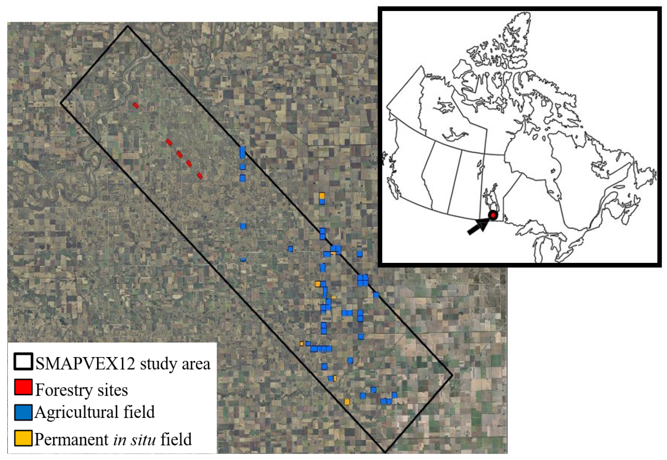
2.1. Materials

The study site corresponds to the site that was used in the Soil Moisture Active Passive Validation Experiment 2012 (SMAPVEX12) campaign [7]. It is located in the trans-boundary Red River Watershed (Province of Manitoba), in western Canada (Figure 1). The area is centred on the village of Elm Creek (98°0′23″W, 49°40′48″N), which is near the provincial capital of Winnipeg. The study covers an area of about 15 km by 70 km, and consists mainly of farmland and a few forested areas (dominated by trembling aspen, burr oak and balsam poplar) [7]. Many annual crops are grown here, including wheat, maize (corn), soybeans, beans, barley and canola (edible rapeseed), together with perennial land covers (including grass and alfalfa pastures). Details are available from the dedicated website (https://smapvex12.espaceweb.usherbrooke.ca/, accessed on 7 October 2023).

The field data that were used in the study originate from the SMAPVEX12 campaign, which was conducted 7 June to 19 July 2012 [7]. The data were collected from 55 fields that were covered by different crops (wheat, soybean, maize, canola, etc.). Soil textures differed across fields in terms of the proportions of sand, silt and clay, ranging from heavy clays to fine sandy loams. Several variables were measured in situ, including soil moisture (mv), surface roughness, dry biomass, crop height and biomass water content. For mv measurements, each field was sampled at sixteen points, which were distributed along two transects. On each acquisition date, three measurements were taken at each point to within 6 cm of the surface, using portable Theta (Delta-T Devices, Burwell, Cambridge, UK) and Hydra (Beaverton, OR, USA) probes. Volumetric soil moisture that was acquired by the probes was calibrated against the gravimetric soil moisture measurements of the soil samples that had been collected. At the same time, additional soil moisture measurements were acquired using automated stations that had been installed in the study area. These sensors form a permanent network of stations that is operated by Agriculture and Agri-Food Canada (AAFC). Data were also taken from temporary networks established by the Manitoba Department of Agriculture, and by the United States Department of Agriculture (USDA).

This study focuses solely upon wheat fields from the SMAPVEX12 campaign (13 fields in total). Several data types were taken on this crop during its growth between 11 June and 18 July 2012, thereby motivating our choice to work on wheat in this research. For instance, roughness data (height s, correlation-length l) were measured using a three-meter-long pin-profilometer in the viewing direction of RADARSAT-2. Mean values found for wheat fields are, respectively, s = 0.99 ± 0.30 cm, and l = 11.29 ± 4.11 cm. Figure 2 shows average moisture in the wheat fields (portable probe measurements), the average rainfall accumulated every six hours, and the average temporal soil moisture profile obtained from automatic station measurements. Soil moisture is particularly high at the start of the campaign, due to the rainfall episodes that were recorded. After Julian day 172, fields gradually dry out until day 188. After this date, a slight moistening occurs until day 196. Rainfall at the end of the season subsequently increases mv variability.

Figure 3 provides a visual illustration of wheat condition during progressive stages of its growth, from stem elongation to ripening. Related dry biomass follows a nearly linear trend from the beginning of the season to ripening (min = 0.105 kg/m², max = 1.241 kg/m², mean = 0.696 ± 0.272 kg/m²). Plant height (h) and water content (VWC) increase almost linearly, right up to the initiation of heading stage (days 175–180). After this period, h increases very slightly due to the seed heads, while VWC decreases. Over the entire campaign, h varied between 29.7 and 106.3 cm, with a mean of 72.2 ± 19.5 cm, while VWC ranged from 0.331 to 3.256 kg/m², with an average value of 2.136 ± 0.640 kg/m².

As part of SMAPVEX12, polarimetric C-band (5.4 GHz) images were acquired by RADARSAT-2 between 5 June and 13 July 2012, in parallel with field measurements. The images were taken in fine mode and quad polarization (HH+HV+VH+VV), with a maximum spatial resolution of 12 m (

Table 1. SMAPVEX12 RADARSAT-2 images used in the study.

Date (mm/dd)	Julian Day (DOY)	Local Time	Angle of Incidence (°)
06/05	157	7:57 a.m.	20–23.6
06/12	164	7:53 a.m.	26.1–29.4
06/12	165	7:15 p.m.	28.4–31.6
06/19	172	7:11 p.m.	23.7–27.2
06/26	179	7:07 p.m.	19–22.7
06/29	181	7:57 a.m.	20–23.6
07/06	188	7:53 a.m.	26.1–29.4
07/06	189	7:15 p.m.	28.4–31.6
07/13	196	7:11 p.m.	23.7–27.2

). For each date, several images were taken a few seconds apart to cover the entire SMAPVEX12 study site.

Complementary auxiliary data were acquired to enable pre-processing of the radar images, e.g., geometric corrections and ortho-rectification. These include Canadian Vector data (CanVec) available on the Canadian government platform Geogratis [39]. Vector layers that were considered are roads, hydrography and vegetation. The CanVec product has a planimetric accuracy of 10 m. Canadian Digital Elevation Data (CDED) were also acquired, at a scale of 1:50,000. They have a planimetric accuracy of 10 m, and a vertical accuracy of 5 m [40].

2.2. Methods

The approach used in this study was (1) to determine the most sensitive non-polarimetric and polarimetric variables and (2) to develop statistical models for estimating soil moisture in wheat fields over the growing season. The various steps in the methodological approach are summarized in Figure 4.

2.2.1. Temporal Interpolation of In Situ Measurements

During the SMAPVEX12 campaign, there were situations where delays existed between satellite overpass and in situ data acquisition times. Analysis of continuous soil moisture (mv) profiles revealed that the error associated with a 24 h acquisition delay was in the order of 0.010 m³/m³, which constitutes a very small error. However, on several days when RADARSAT-2 passed over the study site, the corresponding mv measurement was delayed by more than 24 h. To correct for the delay and to collect as many data points as possible for the analysis, we used a temporal interpolation. Thus, for each wheat field, a linear relationship was established between mv measurements acquired by hand-held probes and those of the nearest automated station. This relationship was then used to estimate the average mv value for the field from the mv values measured by the automated station at the time of RADARSAT-2 overpass. Only highly significant relationships (p ≤ 0.01) were considered, to avoid propagating large errors in the soil moisture values considered for model development (calibration) and validation.

Soil roughness was considered to be constant across the same field throughout the campaign. Thus, no interpolations were conducted on roughness measurements. Vegetation measurements (biomass, height, water content) with acquisition delays of less than one day relative to the corresponding radar image were used without interpolation. Values were linearly interpolated for time lags that were greater than 1 day. This approach was justified by the quasi-linear temporal profiles of the various variables that were measured during the SMAPVEX12 campaign.

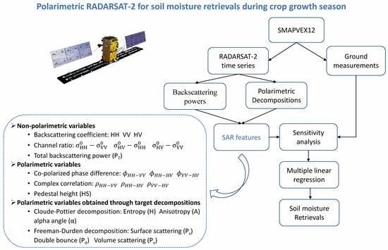
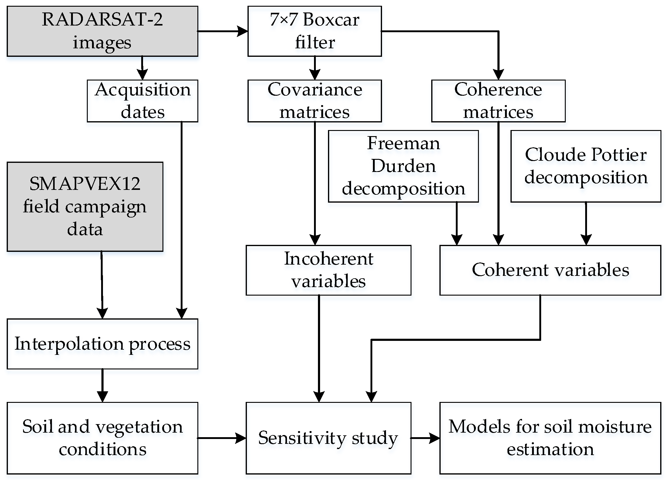
2.2.2. Processing of RADARSAT-2 Images

The complete polarimetric description of the RADARSAT-2 signal is provided by the Sinclair matrix [S], which is composed of complex values (S_ij) representing the signal in incident i and received j polarizations [41]. In linear polarization, i and j are horizontal (H) or vertical (V). Therefore:

$$[S]=\left[\begin{array}{cc}{S}_{HH}& S_{HV}\\ S_{VH}& S_{VV}\end{array}\right]$$

(1)

This diffusion matrix can be explained as vectors $\underset{\_}{k}$ or $\underset{\_}{\mathsf{\Omega }},$ such that:

$$\underset{\_}{k}=\frac{1}{\sqrt{2}}{\left[S_{HH}+S_{VV}{S}_{HH}-S_{VV}2S_{\mathrm{H}\mathrm{V}}\right]}^T$$

(2)

$$\underset{\_}{\mathsf{\Omega }}={\left[S_{HH}\sqrt{2}{S}_{HV}{S}_{VV}\right]}^T$$

(3)

The covariance $\left[C_3\right]$ and coherence $\left[T_3\right]$ matrices for a target then can be calculated as:

$$\left[C_3\right]=〈\underset{\_}{\mathsf{\Omega }}·{\underset{\_}{\mathsf{\Omega }}}^{\mathrm{*}T}〉=\left[\begin{array}{ccc}〈{\left|S_{HH}\right|}^2〉& \sqrt{2}〈S_{HH}{S}_{HV}^{\mathrm{*}}〉& 〈S_{HH}{S}_{VV}^{\mathrm{*}}〉\\ \sqrt{2}〈S_{HV}{S}_{HH}^{\mathrm{*}}〉& 〈{\left|S_{HV}\right|}^2〉& \sqrt{2}〈S_{HV}{S}_{VV}^{\mathrm{*}}〉\\ 〈S_{VV}{S}_{HH}^{\mathrm{*}}〉& \sqrt{2}〈S_{VV}{S}_{HV}^{\mathrm{*}}〉& 〈{\left|S_{VV}\right|}^2〉\end{array}\right]$$

(4)

$$\begin{array}{c}\left[T_3\right]=〈\underset{\_}{k}·{\underset{\_}{k}}^{\mathrm{*}T}〉=\hfill \\ \hfill 1/2\left[\begin{array}{ccc}〈{\left|S_{HH}{+S}_{VV}\right|}^2〉& 〈{\left(S_{HH}+S_{VV}\right)\left(S_{HH}-S_{VV}\right)}^{\mathrm{*}}〉& 2〈\left(S_{HH}+S_{VV}\right)S_{HV}^{\mathrm{*}}〉\\ 〈{\left(S_{HH}-S_{VV}\right)\left(S_{HH}+S_{VV}\right)}^{\mathrm{*}}〉& 〈{\left|S_{HH}{-S}_{VV}\right|}^2〉& 2〈\left(S_{HH}-S_{VV}\right)S_{HV}^{\mathrm{*}}〉\\ 2〈S_{HV}{\left(S_{HH}+S_{VV}\right)}^{\mathrm{*}}〉& 2〈S_{HV}{\left(S_{HH}-S_{VV}\right)}^{\mathrm{*}}〉& 4〈{\left|S_{HV}\right|}^2〉\end{array}\right]\hfill \end{array}$$

(5)

where the operator * refers to the conjugate of the complex value and the operator 〈...〉 refers to the mean value on the target surface. The HH, HV and VV polarised backscattering coefficients correspond to the diagonal elements of the covariance matrix $\left[C_3\right]$. Several polarimetric variables can be estimated from the complex elements [41]. In this study, linear backscattering coefficients were obtained from grey levels by calibration using the Look-Up Tables accompanying RADARSAT-2 products. Covariance and coherency matrices $\left[C_3\right]$ and $\left[T_3\right]$ were generated from the calibrated products, using PolSARpro (version 5), available in Geomatica software 2016. We then used a Boxcar 7 × 7 filter [42] to reduce speckle, which can otherwise create biases on variables that are derived from polarimetric decompositions [43]. This filter was applied to the images of the complex matrix terms $\left[C_3\right]$ and $\left[T_3\right]$, prior to extraction of radar variables that were used in subsequent analyses. A total of seven non-polarimetric variables were extracted from the filtered covariance matrix (

Table 2. List of non-polarimetric and polarimetric variables that were considered in the study.

Non-Polarimetric Variables (dB)
Backscattering coefficient HH (${\sigma }_{HH}^0$); Backscattering cross-coefficient HV (${\sigma }_{HV}^0$); Backscattering coefficient VV (${\sigma }_{VV}^0$); Channel ratio HH-VV (${\sigma }_{HH}^0-{\sigma }_{VV}^0)$; Channel ratio HV-HH (${\sigma }_{HV}^0-{\sigma }_{HH}^0$); Channel ratio HV-VV (${\sigma }_{HV}^0-{\sigma }_{VV}^0$); Total backscattering power (PT).
Polarimetric Variables
Co-polarized phase difference (${\varphi }_{HH-VV}$); Complex co-polarized channel correlation (${\rho }_{HH-VV}$); Cross-polarization phase differences (${\varphi }_{HH-HV}$, ${\varphi }_{VV-HV}$); Complex cross-polarization channels (${\rho }_{HH-HV}$, ${\rho }_{VV-HV}$); Pedestal height (HS).
Polarimetric Variables Obtained through Target Decomposition
Cloude–Pottier decomposition: Entropy (H), anisotropy (A), alpha-angle (α); Freeman–Durden decomposition: Surface component (Ps), Interaction component (Pd), Volume component (Pv).

). The ${\sigma }^0$ values were then converted to amplitudes (dB) using Equation (6):

$${\sigma }^0\left(\mathrm{d}\mathrm{B}\right)={10}^{·}{\log }_{10}{[\sigma }^0\left({\mathrm{c}\mathrm{m}}^2/\mathrm{c}{\mathrm{m}}^2\right)]$$

(6)

where ${\sigma }^0$ is the backscatter coefficient. Polarimetric variables were calculated from coherence and covariance matrices of targets for each image, using PolSARpro. Furthermore, 13 polarimetric variables were extracted, including six that were derived from the Cloude–Pottier and Freeman–Durden decompositions. Table 2 summarizes the sets of variables extracted from RADARSAT-2 images for the purposes of this study.

Images of the different variables were subjected to a process of geometric correction and ortho-rectification. This step is necessary to locating study fields precisely and, subsequently, to extract their corresponding values. The operations were performed with the hybrid model that was proposed by Toutin [44], using DEM (digital elevation model) and vector data described in Section 2.1 Inclusion of vector files for the roads ensured the quality of the georeferencing.

2.2.3. Sensitivity Study and Modelling

Once variable values had been extracted from the various fields, a sensitivity study was conducted to understand the effects of individual contributions of measured soil and vegetation characteristics on the radar signal, together with the interrelationships between the different radar variables. Sensitivity was assessed in each case by examining the correlation coefficient r and its level of statistical significance (p-value). To be considered for inclusion in model development, non-polarimetric and polarimetric variables had (1) to exhibit a significant correlation with mv (p < 0.05), and (2) to exhibit no collinearity with other explanatory radar variables (r < 0.9). This threshold was adopted after several trials with different r values varying from 0.50 to 0.95. In the event of collinearity, only the explanatory variable with the highest significant correlation with mv was retained.

Once explanatory radar variables were selected, we proceeded to develop empirical models to estimate soil moisture and to highlight the contribution of polarimetry. The general formulation of the proposed multiple linear models is given by Equation (7). These models use a set of explanatory variables X_i (polarimetric or non-polarimetric) among those that had been selected during the sensitivity study, such that:

$$m_v={\beta }_1{X}_1+\dots +{\beta }_i{X}_i+\dots +{\beta }_p{X}_p+{\beta }_0+ϵ$$

(7)

Calibration coefficients β_i were determined by multiple linear regression. A model can be calibrated with or without an intercept (β₀), and an error term 𝜖. Three models were proposed. The first model is entirely non-polarimetric. It was developed using ${\sigma }_{HH}^0$, ${\sigma }_{HV}^0$ and ${\sigma }_{VV}^0$. The second model was based upon multiple linear regression and constructed with the set of polarimetric and non-polarimetric variables retained following the sensitivity study. Finally, the third model was proposed with a view to reducing the number of explanatory variables being considered. It was based on stepwise regression, to retain only the most relevant explanatory polarimetric and non-polarimetric variables.

2.2.4. Calibration and Validation of the Models

We divided the available wheat field observations into two groups. The first group comprised the training or calibration set, which was used to determine the calibration coefficients βi of the models, together with their significance levels. The second group was used for independent validation of the results. Each group covered the widest possible range of values for the characteristics measured in the fields. To meet this objective, we used Kolmogorov–Smirnov and t-tests to evaluate the hypothesis that the two sample groups belonged to the same population and followed similar distributions. Goodness-of-fit of each model was verified by inspecting residuals of the estimates, especially their normality, linearity and homoscedasticity (i.e., equality of residual variances). During both phases (calibration and validation), model strength was assessed using correlation, significance level (p-value), and root-mean-square error (RMSE) between estimated and measured soil moisture.

3. Results

This section summarizes the main results found following the application of the methodological scheme proposed, as shown in Figure 4.

3.1. Temporal Interpolation

This operation was required to obtain in situ soil moisture values in the wheat fields for several RADARSAT-2 overpasses during the campaign. Overall, the linear interpolation models were highly significant (

Table 3. Statistics of linear interpolation of soil moisture (mv) for each wheat field. A distance of 0 km indicates that the station is located in the field. r is the correlation coefficient, p-value is the level of significance of the relationship, RMSE is the root-mean-square error interpolated mv.

	Meteorological Station
Field ID	Network	Distance (km)	r	p-Value	RMSE (m3/m3)
73-1	USDA	1.0	0.871	0.00	0.018
74-1	USDA	0.0	0.929	0.00	0.015
104	USDA	0.0	0.971	0.00	0.027
105	USDA	0.8	0.974	0.00	0.018
31	USDA	0.0	0.912	0.00	0.033
32	Sages	0.0	0.774	0.00	0.062
44	USDA	0.8	0.885	0.00	0.036
45	USDA	0.0	0.875	0.00	0.044
55	USDA	0.0	0.888	0.00	0.037
81	USDA	0.0	0.911	0.00	0.018
85	USDA	3.7	0.716	0.01	0.037
91	USDA	0.0	0.910	0.00	0.020

; p < 0.01), with low RMSE errors. Accordingly, the results were considered sufficiently robust and satisfactory, and were used to increase the number of soil moisture observations. Sixty observations (eight wheat fields) constituted the calibration set. The validation set was comprised of 40 observations (5 fields).

3.2. Sensitivity Analysis and Variable Selection

Table 4. Correlations between non-polarimetric and polarimetric variables derived from RADARSAT-2 data and agricultural field characteristics, including soil moisture (mv), surface roughness height (s), surface roughness correlation length (l), vegetation biomass (V_B), average wheat height (h) and water content (VWC). Yellow indicates non-significant (0.05 < p < 0.10), Orange significant (0.01 < p < 0.05) and Green very significant (0 < p < 0.01) relationships. See Table 2 for definitions of radar variables.

	Non-Polarimetric Variables
	${\sigma }_{HH}^0$	${\sigma }_{HV}^0$	${\sigma }_{VV}^0$	PT	${\sigma }_{HH}^0-{\sigma }_{VV}^0$	${\sigma }_{HV}^0-{\sigma }_{HH}^0$	${\sigma }_{HV}^0-{\sigma }_{VV}^0$
mv	0.33	0.56	0.53	0.49	−0.24	0.34	0.19
s	0.10	−0.10	0.06	0.08	0.02	−0.23	−0.20
l	−0.22	0.20	0.03	−0.09	−0.22	0.48	0.20
VB	−0.07	−0.18	−0.25	−0.15	0.20	−0.10	0.10
h	−0.27	−0.35	−0.52	−0.42	0.28	−0.10	0.13
VWC	−0.15	−0.30	−0.34	−0.25	0.20	−0.12	0.06
	Non-Polarimetric Variables
	${\rho }_{HH-HV}$	${\varphi }_{HH-HV}$	${\rho }_{HH-VV}$	${\varphi }_{HH-VV}$	${\rho }_{VV-HV}$	${\varphi }_{VV-HV}$	HS
mv	0.00	−0.06	−0.02	−0.64	−0.01	0.06	0.33
s	−0.08	−0.02	0.12	0.25	0.04	0.07	−0.28
l	0.22	0.14	−0.04	−0.11	0.21	−0.13	0.40
VB	−0.25	−0.03	−0.16	0.41	−0.15	0.13	−0.10
h	−0.26	0.09	−0.24	0.53	−0.17	−0.01	−0.04
VWC	−0.19	0.05	−0.17	0.14	−0.23	0.08	−0.10
	Variables from Target Decomposition
	H	A	α	${\mathit{P}}_{\mathit{s}}$	${\mathit{P}}_{\mathit{v}}$	${\mathit{P}}_{\mathit{d}}$
mv	0.29	−0.34	0.01	0.13	0.50	−0.14
s	−0.26	0.25	−0.08	0.22	−0.12	0.21
l	0.35	−0.21	0.09	−0.42	0.19	−0.26
VB	−0.07	0.10	0.36	−0.12	−0.12	0.03
h	−0.01	0.06	0.35	−0.33	−0.25	0.00
VWC	−0.07	0.16	0.24	−0.09	−0.22	0.01

summarizes the results found. The link is significant between mv and non-polarimetric variables in general. Yet, some of these variables are also sensitive to the wheat biomass, height and water content; as well as surface roughness, i-e correlation-length and height (Table 4). This observation is likewise valid for the polarimetric variables. The phase difference ϕ_HH−VV shows the most significant inverse correlation with mv (R = −0.64, p < 0.05), but it is also very positively related to wheat height h.

Based on Table 4, we can count a dozen potentially interesting variables for estimating soil moisture. By discarding backscattering ratios (linked to backscattering coefficients) and taking into account collinearities (P_T vs. ${\sigma }_{HH}^0$, entropy H vs. pedestal height HS, P_V vs. ${\sigma }_{HV}^0),$ we retained six variables for the development of multiple linear models. These are three non-polarimetric variables (${\sigma }_{HH}^0$, ${\sigma }_{HV}^0 \mathrm{a}\mathrm{n}\mathrm{d} {\sigma }_{VV}^0$) and three polarimetric variables (ϕ_HH−VV, H_S $\mathrm{a}\mathrm{n}\mathrm{d}$ A).

3.3. Non-Polarimetric Model

This model was developed in two iterations. The first calibration simultaneously considered the three backscattering coefficients (${\sigma }_{HH}^0$, ${\sigma }_{HV }^0\mathrm{a}\mathrm{n}\mathrm{d}{\sigma }_{VV}^0$). It permitted the development of a preliminary model referred to as 3_Sigma. Analysis showed that the only terms of this 3_Sigma model that demonstrated significance were the intercept and ${\sigma }_{HV}^0$ (

Table 5. Parameters of empirical linear models based solely upon non-polarimetric variables. Model 3_Sigma includes intercept and all three back-propagation coefficients (${\sigma }_{HH}^0, {\sigma }_{HV}^0, {\sigma }_{VV}^0$). Model Sigma_Hv is based only on significant variables (p < 0.05); i.e., the intercept and ${\sigma }_{HV}^0$. β_i are the regression coefficients (see general formulation in Equation (7)), r is the correlation coefficient, and RMSE is the root-mean-square error.

Model	Number of Fields	Number of Observations	r	RMSE (m3/m3)	Variable	βi	Standard Error	p-Value
3_Sigma	8	60	0.59	0.096	(Intercept)	1.101	14%	0.000
					${\sigma }_{HH}^0$	0.001	793%	0.900
					${\sigma }_{HV}^0$	0.047	29%	0.001
					${\sigma }_{VV}^0$	−0.001	−1426%	0.944
Sigma_HV	8	60	0.60	0.095	(Intercept)	1.153	14%	0.000
					${\sigma }_{HV}^0$	0.050	18%	0.000

). We conducted a second calibration that considered these two terms. The resulting non-polarimetric model (denoted Sigma_Hv) is well conditioned, given that its residuals satisfy normality and homoscedasticity assumptions (Table 5, Figure 5). RMSE error is 0.095 m³/m³, and all terms are significant (Table 5). For the remainder of the study, only the Sigma_Hv model is considered as a non-polarimetric model and compared to other models that were developed.

3.4. Models Based upon Non-Polarimetric and Polarimetric Variables

The first model that was developed is based upon multiple regression that considers all six non-polarimetric and polarimetric variables, which were selected during the sensitivity analysis (Section 3.2). This model is referred to as a mixed polarimetric model or MixPol in the text. All β_i coefficients obtained for the MixPol model are significant (p < 0.05), as indicated in

Table 6. Coefficients of multiple linear regression (i.e., MixPol model) and simplified stepwise regression SPol model.

Model	Number of Fields	Number of Observations	r	RMSE (m3/m3)	Variables	βi	Std. βi	Standard Error	p-Value
MixPol	8	60	0.77	0.078	${\sigma }_{HH}^0$	0.107	0.129	16%	0.000
					${\sigma }_{HV}^0$	−0.117	−0.177	−23%	0.000
					${\sigma }_{VV}^0$	0.057	0.076	34%	0.005
					${\varphi }_{HH-VV}$	−0.003	−0.057	−24%	0.000
					Hs	2.072	0.082	15%	0.000
					A	−1.637	−0.067	−36%	0.008
SPol	8	60	0.71	0.084	Intercept	0.662	0.662	12%	0.000
					${\sigma }_{HH}^0$	0.036	0.043	26%	0.000
					${\varphi }_{HH-VV}$	−0.004	−0.076	−14%	0.000

. Its RMSE error (0.078 m³/m³) is lower than that of Sigma_Hv and, likewise, its correlation is higher (r = 0.77 vs. r = 0.60). The histogram of residuals and the normal probability plot, together with observed homoscedasticity in the distribution of residuals (vs. predicted mv), indict that MixPol is well conditioned (Figure 6a).

The major drawback of the MixPol model is the large number of variables. Thus, we developed a second model combining the two categories of variables by applying stepwise regression, to reduce the number of the variables, while maintaining a level of performance similar to that of the MixPol model. The simplified model that was obtained, denoted the SPol model, contains a non-polarimetric variable (${\sigma }_{HH}^0$) and a polarimetric variable (${\varphi }_{HH-VV}$). According to the distribution of the residuals, it is well conditioned, and all its coefficients are highly significant. RMSE error (0.084 m³/m³) and the correlation (r = 0.714) are comparable to those obtained with the six-variable MixPol model (Table 6; Figure 6b).

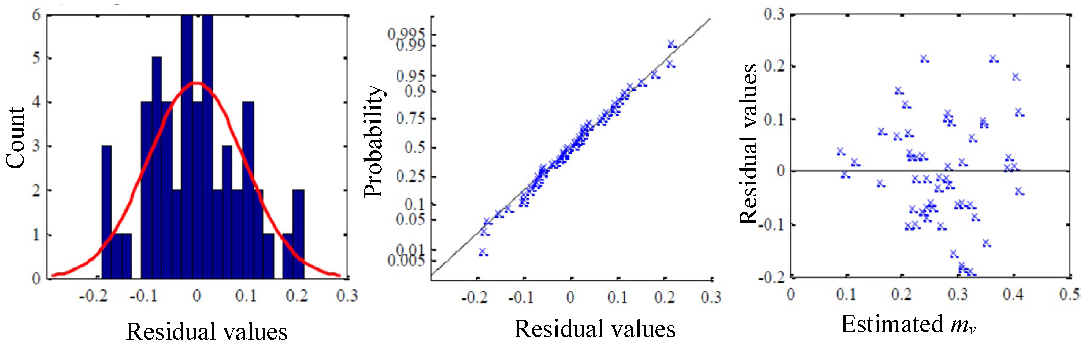
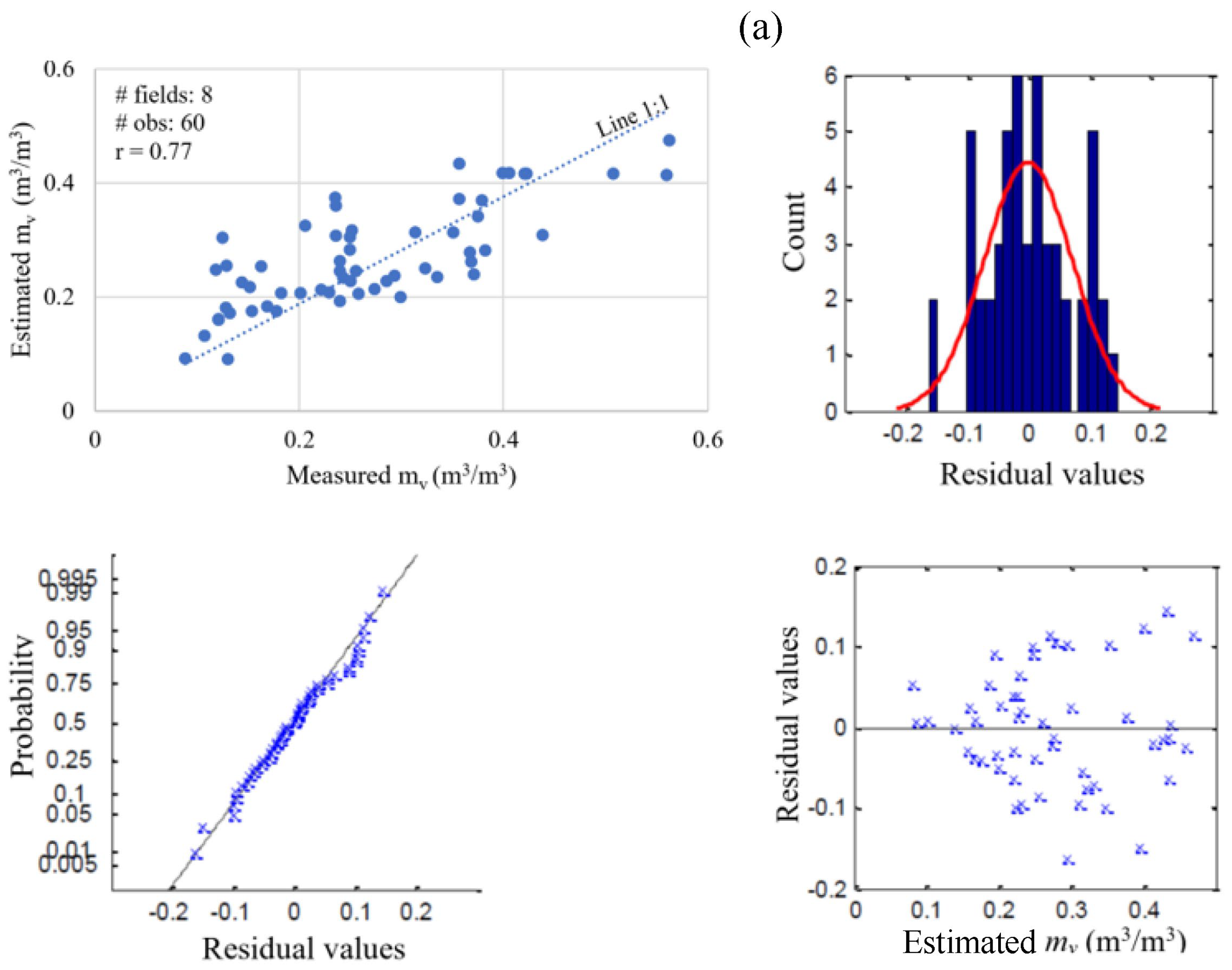
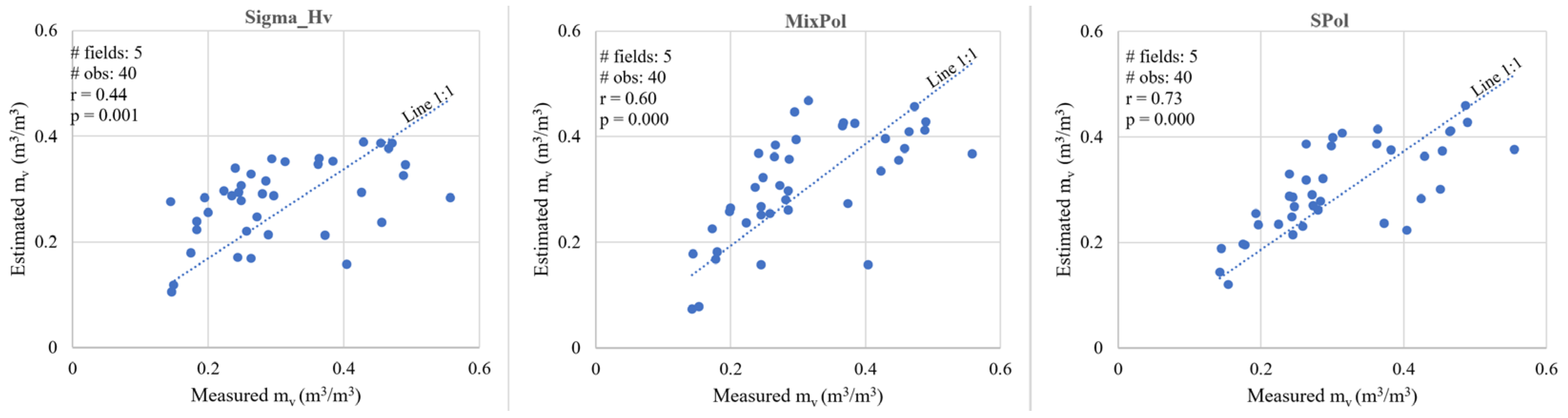
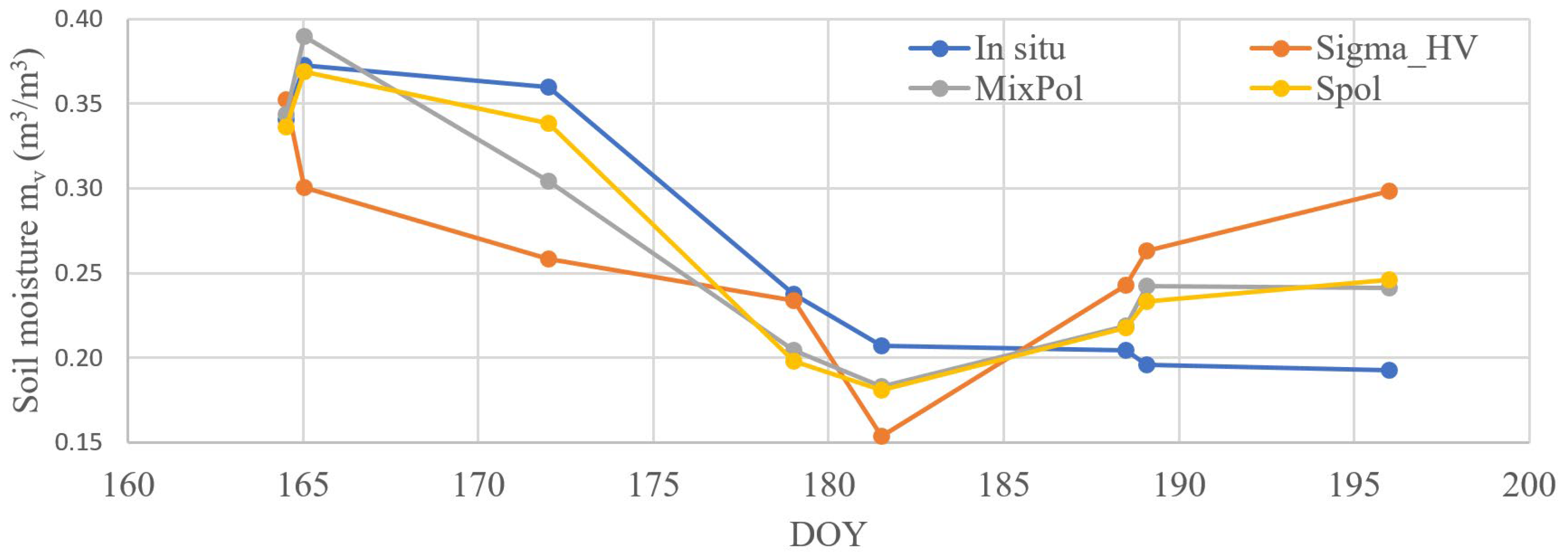
3.5. Validation of Models

The three models were validated using observations from the five independent wheat fields that were reserved for validation (see Section 2.2), totaling 40 observations. Figure 7 shows the comparison of measured and estimated soil moisture values. The non-polarimetric model (Sigma_Hv) exhibits the poorest performance (RMSE = 0.098 m³/m³), compared to the polarimetric models MixPol and Spol (RMSE range: 0.074 m³/m³ to 0.087 m³/m³).

Following validation, we established average temporal profiles of soil moisture estimated by the three models on all wheat fields, and we compared them to averages of in situ measurements (Figure 8). The three models exhibit negative residual bias after the start of the campaign until flowering, and positive bias during grain development and ripening. The behavior of this bias appears to be consistent with wheat growth stages, suggesting a residual influence of land cover on model performance. Overall, the non-polarimetric model exhibits the greatest biases and, therefore, seems more sensitive to the presence of vegetation than do the polarimetric models.

4. Discussion

4.1. Match between Satellite Observation and Ground Measurements

This study benefited from the scope of the SMAPVEX12 campaign [7], with the advantage of covering the principal stages of wheat growth in terms of in situ measurements and polarimetric RADARSAT-2 images. Yet, environmental conditions during the campaign influenced the dynamics of vegetation development and soil characteristics. In fact, significant rainfall occurred at the beginning of the campaign, resulting in higher soil moisture. Thereafter, subsequent bouts of rain were rare. Consequently, the fields dried up while the wheat shoots were growing. This coincidence incurred significant negative correlations between soil moisture and biomass, and soil moisture vs. crop height, thereby influencing the measured radar signal.

Moreover, for more than half of the fields that were overflown by the satellite, soil moisture was measured in the field with a lag with respect to date of acquisition of the nearest RADARSAT-2 image. Instead of discarding these values, we used a temporal interpolation method to estimate soil moisture during the missing flyover times. This gap-filling method, which was based upon a linear relationship that was specific to each field, took advantage of the regular hourly measurements that had been acquired by the automated stations. Interpolation proved to be very robust, with errors being sufficiently small (mostly < 0.04 m³/m³, Table 3) as not to influence the development of soil moisture estimation models. Overall, the availability of RADARSAT-2 close to ground measurements time during the SMAPVEX12 field works was limited, thus reducing the number of samples considered in the development of the models proposed. Also, with the limited dataset, using approaches such as machine learning methods is difficult to envisage.

4.2. Sensitivity Analysis

The sensitivity analysis that was carried out reveals a significant relationship between soil moisture and backscattering in the three linear polarizations (Table 4). Although it is generally admitted that backscattering coefficients are sensitive to soil moisture, it is important to notice that the relations could be influenced by many factors such as soil type, conditions, roughness, level of humidity, vegetation, etc. Sensitivity of ${\sigma }_{HV}^0$ to mv, which is the highest found here, depends upon the stage of field crop development (figure not shown). Indeed, mv is responsible for most of the backscatter signal ($R_{HV}=0.62$) between the start of the campaign (day 157) and the start of grain development (around day 180). The linkage between ${\sigma }_{HV}^0$ and soil moisture is known for bare soils (e.g., Oh [24], semi-empirical model). Bare soils contributions are dominant at the first stages of wheat growth period. In addition, wheat fields may show discernable rows during their growth stages, thus allowing possible contributions of underlying ground, as well as double bounce and volume scattering. From grain development until the end of the campaign (day 201), dry biomass increases with the development of the plant head and is responsible for most of the signal ${\sigma }_{HV}^0$ (correlation of 0.56 vs. 0.34 for soil moisture). These observations are supported by literature reports, given that the change in backscattering dynamics with the appearance of the heads had already been observed for co-polarized linear channels [45,46,47].

At the level of polarimetry, the phase difference ϕ_HH−VV showed the strongest sensitivity to mv. ϕ_HH−VV contains information related to the microwave propagation path [47,48]. In general, over agricultural fields, the backscattered signal could have a variety of co-polarized phase difference values, due to many factors related to soil and crop (type, structure, density and growing stage). ϕ_HH−VV will account for the propagation difference occurring during the travel of the signal through the vegetation volume, and the process will be largely influenced by the orientations of the crop elements. Jagdhuber [49] provides more insights on the impact of ϕ_HH−VV and indicates that its contribution can be hardly neglected in situations where media are strongly oriented. Indeed, neglecting ϕ_HH−VV means that the vegetation volume structure is randomly oriented, and anisotropies are quite inexistent. This may not be fair for crops like wheat with vertical stalks favorable to dihedral scattering creating variations in ϕ_HH−VV [38]. The total ϕ_HH−VV may be a complex variable that can have three primary phase difference components due to two-way propagation through the vegetation layer, Fresnel reflection by soil surface, and bistatic scattering by stalks [50]. This is exacerbated in canopies with a standing structure (such as wheat), where the distribution of ϕ_HH−VV values becomes important. In this study, a negative correlation is observed between ϕ_HH−VV and soil moisture, while positive correlations were found with surface roughness, as well as wheat biomass and height. This translates to a clear contribution of the surface, but also to the presence of significant volume scattering and double bounce [50,51]. This latter may be due to the penetration of one of the polarizations between the rows in the wheat fields [52,53]. Consequently, a direct physical interpretation of the relationships between ϕ_HH−VV and the different surface properties, including soil moisture, may not be straightforward, and could require a modelling framework.

After ϕ_HH−VV, the volume power Pv, which is derived from the Freeman–Durden decomposition, also shows a significant correlation with mv. Yet, the strong correlation of Pv with soil moisture, rather than with vegetation characteristics, appears paradoxical. It could be explained by the fact that Ps was obtained by inversion of the Bragg scattering model; according to its formulation, the Bragg model ignores the effects of ground depolarization [48]. In all cases, Pv was discarded because of its collinearity with ${\sigma }_{HV}^0$ (r = 0.97).

Among the variables derived from the Cloude–Pottier decomposition, only anisotropy and pedestal height were retained. The sensitivity of anisotropy to mv indicates that the dielectric properties of the soil contribute to the radar signal as a secondary scattering mechanism [48]. Pedestal height also exhibits a significant link with mv. Yet, just like the anisotropy, it is influenced by the roughness of the ground surface. The α-angle strongly depends upon the vegetation, rather than on mv. Therefore, this variable was not retained.

4.3. Selection of SAR Parameters for Empirical Models

This study aims to evaluate and analyze various SAR variables to characterize soil moisture. No priority was established a priori for the selection of absolute values of the backscattering powers, ratios between channels or polarimetric variables. The strategy was to evaluate the contributions of all potential variables that can be extracted from radar polarimetric images to estimate soil moisture. The six variables that were retained following the sensitivity analysis made it possible to propose three statistical models for estimating soil moisture in the wheat fields from RADARSAT-2 data (Table 5 and Table 6, Figure 5 and Figure 6). (1) For non-polarimetric case, the 3_Sigma model was first developed using the three backscattering coefficients (${\sigma }_{HH}^0, {\sigma }_{VV}^0, {\sigma }_{HV}^0$), then the simplified Sigma_HV model was derived by stepwise regression to provide similar performance with only ${\sigma }_{HV}^0$ as a variable. (2) For the polarimetric case, although the MixPol model obtained satisfactory retrieval results, the major drawback was the large number of variables. Thus, we developed a simplified model by applying stepwise regression to reduce the number of input variables, while maintaining a similar performance as the MixPol model. Thus, it was expected that the SPol model shows a similar performance as the MixPol. Therefore, the similarities between the results of polarimetric models (MixPol and Spol) or between those of the non-polarimetric models (3_Sigma and Sigma_HV) is due to the strategy adopted rather than the limitations of data and should not be misinterpreted. Overall, the metrics obtained using only non-polarimetric variables are weaker compared to MixPol and SPol. This shows the valuable contribution of polarimetric variables. For instance, in the SPol model, the stepwise regression retained only ${\sigma }_{HH}^0$ and polarimetric ϕ_HH−VV. The possible physical explanation is that while ${\sigma }_{HH}^0$ contains the effects of both soil moisture and vegetation, ϕ_HH−VV may account for the vegetation contribution. Therefore, its introduction into the model may help to reduce the effects of the vegetation and allow soil moisture retrieval.

In the validation process using the independent dataset, the non-polarimetric model Sigma_Hv, which only depends upon ${\sigma }_{HV}^0$, made it possible to estimate mv with an RMSE error of 0.098 m³/m³, while explaining only 19% of its variance (Figure 7). The HV channel alone summarizes redundant soil moisture information that is contained in the HH and VV channels reasonably well [47]. The dominant contribution of soil at the first stages of the field campaign could explain why ${\sigma }_{HV}^0$ stands out as the main variable in the Sigma_HV model in our study. Recent research by Wang et al. [54], using a more complex approach than our study, over the same SMAPVEX12 study area, also shows the predominant role of ${\sigma }_{HV}^0$ in characterizing the crops and estimating soil moisture. Even if the results that were obtained were statistically significant, the non-polarimetric model would not perform well. Indeed, on the same validation dataset, the MixPol model produced an RMSE of 0.087 m³/m³ and explained almost twice (36.2%) as much of the mv variance. The SPol model demonstrates the best performance during validation, with an RMSE of 0.074 m³/m³, and an explained variance of 53.5% (see Figure 7, Section 3.5). Superior performance of the simplified model, compared to the polarimetric mixed model, could be explained by the inclusion of a small number of variables (i.e., 2 vs. 6), which would serve to reduce the standard error that is associated with the calibration coefficients β_i, thereby increasing model robustness.

Although the SMAPVEX12 campaign covered a large range of soil moisture variations, we faced some limitations in this study in terms of data samples, due partly to the reduced number of Radarsat-2 images collected during the field campaign as close as possible to ground variables measurements. In future works, we will calibrate and validate the developed empirical models using the largest number of experimental datasets as possible, including SMAPVEX12, SMAPVEX16-MB and other international field campaigns. Calibration/Validation could be also improved by performing better spatial distribution analysis in order to tackle the high spatial variability of soil moisture. The actual paper considered only radar data. Other Earth observation data, such as optical data vegetation indices, could be included in future works.

4.4. Bias and Application of the Developed Models

Most of non-polarimetric and polarimetric variables are sensitive to growth stages. For example, variables ϕ_HH−VV in MixPol and Spol models depend greatly on scattering mechanisms between the underlying soil and wheat canopy, which has vertical stalks. At the beginning of the field campaign bare soil was dominant. However, as the plant grows, the co-polarized backscattering tends to augment due to the combination of surface and dihedral scattering, while the cross-polarized backscattering tends to increase with vegetation volume scattering. These dynamics can influence the models’ behaviors. By examining the temporal profiles of estimated values of mv (Figure 8), a negative residual bias can be observed for all models, from the start of the campaign to the stage of grain development, after which the bias then becomes positive. This complex response could be explained by estimates of calibration coefficients β_i that were associated with backscattering, which were too low at the start of the campaign, and too high at the end of the campaign (vegetation effects). A potential improvement would be to identify a polarimetric variable that could weight backscattering effects by phenological stage.

The application of the models on other different sites makes it possible to better evaluate their performance. The results that were obtained here, in terms of RMSE, are comparable to those reported by different studies using more complex methods [36,47,55]. They nevertheless remain lower than the precision target of 0.04 m³/m³, generally targeted and considered suitable for hydrological applications [11]. Part of the problem is inherent in the use of the C band, whose limitations are known in the presence of vegetation. The latter dominates the signal, although it remains sensitive to soil moisture during wheat growth. The approach could be applied using the L-band, which is characterized by better penetration depth.

4.5. Comparison with Recent Studies

The current paper developed multiple linear regression models to retrieve soil moisture. Compared to the physical models, the major limitation of these empirical models is the dependence of the coefficients (Equation (7)) on data characteristics. In most cases, the coefficients need to be calibrated in order to be used in other study sites or different SAR data types. Also, the number of data samples available for this study was relatively limited, which prohibited the development of approaches such as machine learning algorithms, and also restricted further validation. The limited number of samples considered was due to the constraints to having close Radarsat-2 and ground observations, as soil moisture is a dynamic variable that changes rapidly both spatially and temporally. Despite these limitations, the results found remain robust and comparable to many other studies with more complex approaches. We show below in

Table 7. Comparison of statistical metrics obtained using MLR and machine learning models over different study areas.

Models Comparison	Statistical Metrics between Retrieved and Measured mv		References
	R2	RMSE (m3/m3)
Our MLR	0.54	0.074–0.087
Gradient-boosting regression	0.891	0.0875	Nguyen et al. [58]
ANN	0.64	0.040	Singh and Gaurav [59]
Random Forest	0.64	0.0264	Zhao et al. [56]
	0.753 (Asc)/0.671 (Des)	0.045 (Asc)/0.049 (Des)	Dong et al. [57]
Polarimetric decomposition	0.49	0.12	Wang et al. [60]

results reported by various studies over the SMAPVEX12 area. Most of them consider L-Band data, theoretically more sensitive to soil moisture than the RADARSAT-2 data we used. Different approaches are also considered. For instance, with the development of machine learning and deep learning, remote sensing data are being efficiently analyzed and modelled to retrieve geophysical parameters such as soil moisture. In Zhao et al. [56], the farmland surface soil moisture was retrieved by applying feature optimization and machine learning to the radar and optical data. The Random Forest (RF) algorithms using full-polarimetric RADARSAT-2 and Sentinel-2 provided the best retrieval performance with the coefficient of determination R² = 0.64 and a root mean square error (RMSE) = 0.0264 cm³/cm³, in comparison with other machine learning algorithms such as neural network, generalized regression neural network, support vector regression (SVM), back propagation neural network and extreme learning machine. Similarly, the superior retrieval performance of the RF model was observed by Dong et al. [57] using Sentinel-1 radar data over the Tibetan Plateau. In Nguyen et al. [58], the extreme gradient-boosting regression obtained the best performance with R² = 0.891 and RMSE = 0.0875 cm³/cm³, using Sentinel-1, Sentinel-2 and ALOS Digital Surface Model. In Singh and Gaurav [59], the ANN model obtained the most robust statistical metrics with R² = 0.64 and RMSE = 0.040 cm³/cm³, using Sentinel-1/2 and SRTM digital elevation model (DEM).

In addition to machine learning, polarimetric decomposition techniques were used to retrieve soil moisture over the SMAPVEX12 site. Wang et al. [60] analyze the polarimetric decomposition to isolate surface and dihedral scattering components for retrieving the soil moisture of the SMAPVEX12 site, resulting in R² = 0.49 RMSE = 0.12 cm³/cm³ for the wheat fields. Thus, compared to polarimetric decomposition approaches for multiple crops, our current MLR models for wheat fields obtained better statistical metrics.

5. Conclusions

This study assessed the contribution of polarimetry to soil moisture estimation in wheat fields, using RADARSAT-2 C-band images and in situ soil and vegetation measurements taken during the SMAPVEX12 campaign. The C-band radar signal exhibited sensitivity to soil moisture levels in the wheat fields during the growth cycle. This sensitivity is particularly reflected through cross-polarization backscatter ${\sigma }_{HV}^0$, and the phase difference (${\varphi }_{HH-VV}$). The use of explanatory non-polarimetric and polarimetric variables that explained the greatest variation made it possible to develop three statistical models: (1) a one-variable non-polarimetric model variable (${\sigma }_{HV}^0$), (2) a polarimetric mixed model including three non-polarimetric and three polarimetric variables, and (3) a simplified two-variable polarimetric mixed model (${\varphi }_{HH-VV}$, ${\sigma }_{HH}^0$). Validation of the results demonstrated a significant positive contribution of polarimetry, since the two polarimetric models had lower errors (RMSE, range: 0.074 m³/m³ to 0.084 m³/m³, vs. 0.098 m³/m³), and explained two- to three-fold times greater variation in the observed soil moisture than did the non-polarimetric model. A much more pronounced residual bias is present in the temporal soil moisture profile that was estimated by the non-polarimetric model, compared to the polarimetric models. In turn, this bias depends upon the growth stages of the wheat. Future work could improve models by integrating phenology (progressive plant development stages) into a variable weighting the effect of backscattering under changing vegetation cover, to minimize biases that were observable prior to and following wheat heading. Using L-band instead of C-band information could also help improve results. Future works could include the test of all three models using the L-band fully polarimetric data of the upcoming NASA-ISRO Synthetic Aperture Radar (NISAR) mission (launch date in 2024). The analyses carried out here could lead to the development or improvement of more robust semi-empirical or physical models, whose inversion could be used to estimate soil moisture.

References

1. Entekhabi, D.; Rodriguez-Iturbe, I.; Castelli, F. Mutual interaction of soil moisture state and atmospheric processes. J. Hydrol. 1996, 184, 3–17. [Google Scholar] [CrossRef]
2. Jung, M.; Reichstein, M.; Ciais, P.; Seneviratne, S.I.; Sheffield, J.; Goulden, M.L.; Bonan, G.; Cescatti, A.; Chen, J.; de Jeu, R.; et al. Recent decline in the global land evapotranspiration trend due to limited moisture supply. Nature 2010, 467, 951–954. [Google Scholar] [CrossRef] [PubMed]
3. Peng, J.; Albergel, C.; Balenzano, A.; Brocca, L.; Cartus, O.; Cosh, M.H.; Crow, W.T.; Dabrowska-Zielinska, K.; Dadson, S.; Davidson, M.W.J.; et al. A roadmap for high-resolution satellite soil moisture applications—Confronting product characteristics with user requirements. Remote Sens. Environ. 2021, 252, 112162. [Google Scholar] [CrossRef]
4. Sakai, T.; Iizumi, T.; Okada, M.; Nishimori, M.; Grünwald, T.; Prueger, J.; Cescatti, A.; Korres, W.; Schmidt, M.; Carrara, A.; et al. Varying applicability of four different satellite-derived soil moisture products to global gridded crop model evaluation. Int. J. Appl. Earth Obs. Geoinf. 2016, 48, 51–60. [Google Scholar] [CrossRef]
5. Flint, L.E.; Flint, A.L.; Mendoza, J.; Kalansky, J.; Ralph, F.M. Characterizing drought in California: New drought indices and scenario-testing in support of resource management. Ecol. Process. 2018, 7, 1. [Google Scholar] [CrossRef]
6. Lahmers, T.M.; Kumar, S.V.; Locke, K.A.; Wang, S.; Getirana, A.; Wrzesien, M.L.; Liu, P.-W.; Ahmad, S.K. Interconnected hydrologic extreme drivers and impacts depicted by remote sensing data assimilation. Sci. Rep. 2023, 13, 3411. [Google Scholar] [CrossRef] [PubMed]
7. McNairn, H.; Jackson, T.J.; Wiseman, G.; Belair, S.; Berg, A.; Bullock, P.; Colliander, A.; Cosh, M.H.; Kim, S.-B.; Magagi, R.; et al. The Soil Moisture Active Passive Validation Experiment 2012 (SMAPVEX12): Prelaunch calibration and validation of the SMAP soil moisture algorithms. IEEE Trans. Geosci. Remote Sens. 2015, 53, 2784–2801. [Google Scholar] [CrossRef]
8. Martínez-Fernández, J.; González-Zamora, A.; Sánchez, N.; Gumuzzio, A.; Herrero-Jiménez, C.M. Satellite soil moisture for agricultural drought monitoring: Assessment of the SMOS derived Soil Water Deficit Index. Remote Sens. Environ. 2016, 177, 277–286. [Google Scholar] [CrossRef]
9. Cappelletti, L.M.; Sörensson, A.A.; Salvia, M.; Ruscica, R.C.; Spennemann, P.; Fernandez-Long, M.E.; Jobbágy, E. Soil moisture estimates over sporadically flooded farmlands: Synergies and biases of remote sensing and in situ sources. Int. J. Remote Sens. 2022, 43, 6979–7001. [Google Scholar] [CrossRef]
10. Cammalleri, C.; Vogt, J.V.; Bisselink, B.; de Roo, A. Comparing soil moisture anomalies from multiple independent sources over different regions across the globe. Hydrol. Earth Syst. Sci. 2017, 21, 6329–6343. [Google Scholar] [CrossRef]
11. Kerr, Y.H.; Waldteufel, P.; Richaume, P.; Wigneron, J.P.; Ferrazzoli, P.; Mahmoodi, A.; Bitar, A.A.; Cabot, F.; Gruhier, C.; Juglea, S.E.; et al. The SMOS Soil Moisture Retrieval Algorithm. IEEE Trans. Geosci. Remote Sens. 2012, 50, 1384–1403. [Google Scholar] [CrossRef]
12. van der Schalie, R.; Kerr, Y.H.; Wigneron, J.P.; Rodríguez-Fernández, N.J.; Al-Yaari, A.; de Jeu, R.A.M. Global SMOS Soil Moisture Retrievals from The Land Parameter Retrieval Model. Int. J. Appl. Earth Obs. Geoinf. 2016, 45, 125–134. [Google Scholar] [CrossRef]
13. Karthikeyan, L.; Pan, M.; Wanders, N.; Kumar, D.N.; Wood, E.F. Four decades of microwave satellite soil moisture observations: Part 1. A review of retrieval algorithms. Adv. Water Resour. 2017, 109, 106–120. [Google Scholar] [CrossRef]
14. Al-Yaari, A.; Wigneron, J.P.; Kerr, Y.; Rodriguez-Fernandez, N.; O’Neill, P.E.; Jackson, T.J.; De Lannoy, G.J.M.; Al Bitar, A.; Mialon, A.; Richaume, P.; et al. Evaluating soil moisture retrievals from ESA’s SMOS and NASA’s SMAP brightness temperature datasets. Remote Sens. Environ. 2017, 193, 257–273. [Google Scholar] [CrossRef] [PubMed]
15. O’Neill, P.E.; Chan, S.; Njoku, E.G.; Jackson, T.; Bindlish, R.; Chaubell, J. SMAP L3 Radiometer Global Daily 36 km EASE-Grid Soil Moisture; NASA National Snow and Ice Data Center Distributed Active Archive Center: Boulder, CO, USA, 2019. [Google Scholar]
16. Portal, G.; Jagdhuber, T.; Vall-llossera, M.; Camps, A.; Pablos, M.; Entekhabi, D.; Piles, M. Assessment of Multi-Scale SMOS and SMAP Soil Moisture Products across the Iberian Peninsula. Remote Sens. 2020, 12, 570. [Google Scholar] [CrossRef]
17. Ma, H.; Zeng, J.; Chen, N.; Zhang, X.; Cosh, M.H.; Wang, W. Satellite surface soil moisture from SMAP, SMOS, AMSR2 and ESA CCI: A comprehensive assessment using global ground-based observations. Remote Sens. Environ. 2019, 231, 111215. [Google Scholar] [CrossRef]
18. Llamas, R.M.; Guevara, M.; Rorabaugh, D.; Taufer, M.; Vargas, R. Spatial Gap-Filling of ESA CCI Satellite-Derived Soil Moisture Based on Geostatistical Techniques and Multiple Regression. Remote Sens. 2020, 12, 665. [Google Scholar] [CrossRef]
19. Liu, Y.; Yang, Y. Advances in the Quality of Global Soil Moisture Products: A Review. Remote Sens. 2022, 14, 3741. [Google Scholar] [CrossRef]
20. Boerner, W.; Mott, H.; Lueneburg, E.; Livingstone, C.; Brisco, B.; Brown, R.J.; Paterson, J.S. Polarimetry in Radar Remote Sensing: Basic and Applied Concepts; John Wiley & Sons: New York, NY, USA, 1998. [Google Scholar]
21. Dobson, M.C.; Ulaby, F. Microwave Backscatter Dependence on Surface Roughness, Soil Moisture, and Soil Texture: Part III-Soil Tension. IEEE Trans. Geosci. Remote Sens. 1981, GE-19, 51–61. [Google Scholar] [CrossRef]
22. Dobson, M.C.; Ulaby, F.T. Mapping Soil Moisture Distribution with Imaging Radar; John Wiley & Sons: New York, NY, USA, 1998. [Google Scholar]
23. Attema, E.P.W.; Ulaby, F.T. Vegetation modeled as a water cloud. Radio Sci. 1978, 13, 357–364. [Google Scholar] [CrossRef]
24. Oh, Y. Quantitative retrieval of soil moisture content and surface roughness from multipolarized Radar observations of bare soil surfaces. IEEE Trans. Geosci. Remote Sens. 2004, 42, 596–601. [Google Scholar] [CrossRef]
25. Gherboudj, I.; Magagi, R.; Berg, A.A.; Toth, B. Soil moisture retrieval over agricultural fields from multi-polarized and multi-angular RADARSAT-2 SAR data. Remote Sens. Environ. 2011, 115, 33–43. [Google Scholar] [CrossRef]
26. Xing, M.; Chen, L.; Wang, J.; Shang, J.; Huang, X. Soil Moisture Retrieval Using SAR Backscattering Ratio Method during the Crop Growing Season. Remote Sens. 2022, 14, 3210. [Google Scholar] [CrossRef]
27. Gao, L.; Gao, Q.; Zhang, H.; Li, X.; Chaubell, M.J.; Ebtehaj, A.; Shen, L.; Wigneron, J.-P. A deep neural network based SMAP soil moisture product. Remote Sens. Environ. 2022, 277, 113059. [Google Scholar] [CrossRef]
28. Batchu, V.; Nearing, G.; Gulshan, V. A Deep Learning Data Fusion Model using Sentinel-1/2, SoilGrids, SMAP-USDA, and GLDAS for Soil Moisture Retrieval. J. Hydrometeorol. 2023. [Google Scholar] [CrossRef]
29. Zhu, L.; Si, R.; Shen, X.; Walker, J.P. An advanced change detection method for time-series soil moisture retrieval from Sentinel-1. Remote Sens. Environ. 2022, 279, 113137. [Google Scholar] [CrossRef]
30. Evans, D.L.; Farr, T.G.; van Zyl, J.J.; Zebker, H.A. Radar polarimetry: Analysis tools and applications. IEEE Trans. Geosci. Remote Sens. 1988, 26, 774–789. [Google Scholar] [CrossRef]
31. Jiao, X.; McNairn, H.; Shang, J.; Pattey, E.; Liu, J.; Champagne, C. The sensitivity of RADARSAT-2 polarimetric SAR data to corn and soybean leaf area index. Can. J. Remote Sens. 2011, 37, 69–81. [Google Scholar] [CrossRef]
32. Cloude, S.R.; Pottier, E. A review of target decomposition theorems in radar polarimetry. IEEE Trans. Geosci. Remote Sens. 1996, 34, 498–518. [Google Scholar] [CrossRef]
33. Freeman, A.; Durden, S.L. A three-component scattering model for polarimetric SAR data. IEEE Trans. Geosci. Remote Sens. 1998, 36, 963–973. [Google Scholar] [CrossRef]
34. An, W.; Lin, M. An Incoherent Decomposition Algorithm Based on Polarimetric Symmetry for Multilook Polarimetric SAR Data. IEEE Trans. Geosci. Remote Sens. 2020, 58, 2383–2397. [Google Scholar] [CrossRef]
35. Chen, Y.; Zhang, L.; Zou, B.; Gu, G. Polarimetric SAR Decomposition Method Based on Modified Rotational Dihedral Model. Remote Sens. 2023, 15, 101. [Google Scholar] [CrossRef]
36. Wang, H.; Magagi, R.; Goita, K. Comparison of different polarimetric decompositions for soil moisture retrieval over vegetation covered agricultural area. Remote Sens. Environ. 2017, 199, 120–136. [Google Scholar] [CrossRef]
37. Wang, H.; Magagi, R.; Goïta, K.; Colliander, A. Multi-resolution soil moisture retrievals by disaggregating SMAP brightness temperatures with RADARSAT-2 polarimetric decompositions. Int. J. Appl. Earth Obs. Geoinf. 2022, 115, 103114. [Google Scholar] [CrossRef]
38. Shi, H.; Zhao, L.; Yang, J.; Lopez-Sanchez, J.M.; Zhao, J.; Sun, W.; Shi, L.; Li, P. Soil moisture retrieval over agricultural fields from L-band multi-incidence and multitemporal PolSAR observations using polarimetric decomposition techniques. Remote Sens. Environ. 2021, 261, 112485. [Google Scholar] [CrossRef]
39. Natural Resources Canada. Transition Guide NTDB to CanVec; Government of Canada, Natural Resources Canada, Earth and Sciences Sector: Ottawa, ON, Canada, 2013.
40. Natural Resources Canada. Canadian Digital Elevation Model Product Specifications; Government of Canada, Natural Resources Canada, Map Information Branch: Ottawa, ON, Canada, 2016.
41. Lee, J.S.; Pottier, E. Polarimetric Radar Imaging from Basics to Applications; CRC Press: Boca Raton, FL, USA, 2009. [Google Scholar]
42. Lee, J.S.; Ainsworth, T.L.; Kelly, J.P.; Lopez-Martinez, C. Evaluation and Bias Removal of Multilook Effect on Entropy/Alpha/Anisotropy in Polarimetric SAR Decomposition. IEEE Trans. Geosci. Remote Sens. 2008, 46, 3039–3052. [Google Scholar] [CrossRef]
43. López-Martínez, C.; Alonso-González, A.; Fàbregas, X. Perturbation Analysis of Eigenvector-Based Target Decomposition Theorems in Radar Polarimetry. IEEE Trans. Geosci. Remote Sens. 2014, 52, 2081–2095. [Google Scholar] [CrossRef]
44. Toutin, T. Radarsat-2 DSM Generation With New Hybrid, Deterministic, and Empirical Geometric Modeling Without GCP. IEEE Trans. Geosci. Remote Sens. 2012, 50, 2049–2055. [Google Scholar] [CrossRef]
45. Mattia, F.; Toan, T.L.; Picard, G.; Posa, F.I.; Alessio, A.D.; Notarnicola, C.; Gatti, A.M.; Rinaldi, M.; Satalino, G.; Pasquariello, G. Multitemporal C-band radar measurements on wheat fields. IEEE Trans. Geosci. Remote Sens. 2003, 41, 1551–1560. [Google Scholar] [CrossRef]
46. Moran, M.S.; Alonso, L.; Moreno, J.F.; Pilar Cendrero Mateo, M.; Fernando de la Cruz, D.; Montoro, A. A RADARSAT-2 quad-polarized time series for monitoring crop and soil conditions in Barrax, Spain. IEEE Trans. Geosci. Remote Sens. 2012, 50, 1057–1070. [Google Scholar] [CrossRef]
47. Hosseini, M.; McNairn, H. Using multi-polarization C- and L-band synthetic aperture radar to estimate biomass and soil moisture of wheat fields. Int. J. Appl. Earth Obs. Geoinf. 2017, 58, 50–64. [Google Scholar] [CrossRef]
48. Hajnsek, I.; Pottier, E.; Cloude, S.R. Inversion of surface parameters from polarimetric SAR. IEEE Trans. Geosci. Remote Sens. 2003, 41, 727–744. [Google Scholar] [CrossRef]
49. Jagdhuber, T. An Approach to Extended Fresnel Scattering for Modeling of Depolarizing Soil-Trunk Double-Bounce Scattering. Remote Sens. 2016, 8, 818. [Google Scholar] [CrossRef]
50. Ulaby, F.T.; Moore, R.K.; Fung, A.K. Microwave Remote Sensing: Active and Passive, Volume III—Volume Scattering and Emission Theory, Advanced Systems and Applications; Artech House: Norwood, MA, USA, 1986; Volume 3. [Google Scholar]
51. McNairn, H.; Duguay, C.; Brisco, B.; Pultz, T.J. The effect of soil and crop residue characteristics on polarimetric radar response. Remote Sens. Environ. 2002, 80, 308–320. [Google Scholar] [CrossRef]
52. Cable, J.W.; Kovacs, J.M.; Jiao, X.; Shang, J. Agricultural Monitoring in Northeastern Ontario, Canada, Using Multi-Temporal Polarimetric RADARSAT-2 Data. Remote Sens. 2014, 6, 2343–2371. [Google Scholar] [CrossRef]
53. Skriver, H.; Svendsen, M.T.; Thomsen, A.G. Multitemporal C- and L-band polarimetric signatures of crops. IEEE Trans. Geosci. Remote Sens. 1999, 37, 2413–2429. [Google Scholar] [CrossRef]
54. Wang, Z.; Zhao, T.; Qiu, J.; Zhao, X.; Li, R.; Wang, S. Microwave-based vegetation descriptors in the parameterization of water cloud model at L-band for soil moisture retrieval over croplands. GIScience Remote Sens. 2021, 58, 48–67. [Google Scholar] [CrossRef]
55. He, L.; Panciera, R.; Tanase, M.A.; Walker, J.P.; Qin, Q. Soil moisture retrieval in agricultural fields using adaptive model-based polarimetric decomposition of SAR data. IEEE Trans. Geosci. Remote Sens. 2016, 54, 4445–4460. [Google Scholar] [CrossRef]
56. Zhao, J.; Zhang, C.; Min, L.; Guo, Z.; Li, N. Retrieval of Farmland Surface Soil Moisture Based on Feature Optimization and Machine Learning. Remote Sens. 2022, 14, 5102. [Google Scholar] [CrossRef]
57. Dong, L.; Wang, W.; Jin, R.; Xu, F.; Zhang, Y. Surface Soil Moisture Retrieval on Qinghai-Tibetan Plateau Using Sentinel-1 Synthetic Aperture Radar Data and Machine Learning Algorithms. Remote Sens. 2023, 15, 153. [Google Scholar] [CrossRef]
58. Nguyen, T.T.; Ngo, H.H.; Guo, W.; Chang, S.W.; Nguyen, D.D.; Nguyen, C.T.; Zhang, J.; Liang, S.; Bui, X.T.; Hoang, N.B. A low-cost approach for soil moisture prediction using multi-sensor data and machine learning algorithm. Sci. Total Environ. 2022, 833, 155066. [Google Scholar] [CrossRef]
59. Singh, A.; Gaurav, K. Deep learning and data fusion to estimate surface soil moisture from multi-sensor satellite images. Sci. Rep. 2023, 13, 2251. [Google Scholar] [CrossRef]
60. Wang, H.; Magagi, R.; Goita, K.; Jagdhuber, T.; Hajnsek, I. Evaluation of simplified polarimetric decomposition for soil moisture retrieval over vegetated agricultural fields. Remote Sens. 2016, 8, 142. [Google Scholar] [CrossRef]
Figure 1. SMAPVEX12 study area and locations of ground surface measurement points (https://smapvex12.espaceweb.usherbrooke.ca/, accessed on 7 October 2023).
Remotesensing 15 04925 g001
Figure 2. Temporal profiles of volumetric soil moisture (mv) measured by portable probes (box-and-whisker plots; circles superimposed on the boxes are means), daily mean soil moisture recorded by the automated stations (solid line), and mean precipitation (accumulated over 6 h intervals) measured by the meteorological stations above the wheat fields (bar chart).
Remotesensing 15 04925 g002
Figure 3. Photos of wheat plants at different growth stages: (a) stem elongation at day 170; (b) appearance of spike in sheath and end of stem elongation at day 176; (c) heading at day 189; (d) ripening at day 198 (https://smapvex12.espaceweb.usherbrooke.ca/, accessed on 7 October 2023).
Remotesensing 15 04925 g003
Figure 4. Methodological flowchart followed in the study.
Remotesensing 15 04925 g004
Figure 5. Residual values associated with Model Sigma_Hv based on the variable σ H V 0 (Table 5); frequency counts by residual class are compared with a normal distribution with same mean and SD (left-hand panel); close fit of residuals to the 1:1 line in the probability plot suggests the error distribution is normal (middle panel); inspection of residuals vs. predicted values indicate no trends or associations between the two (right-hand panel).
Remotesensing 15 04925 g005
Figure 6. Scatterplot and residual error values associated with MixPol (a) and SPol models (b).
Remotesensing 15 04925 g006aRemotesensing 15 04925 g006b
Figure 7. Validation of the different regression models.
Remotesensing 15 04925 g007
Figure 8. Comparison of estimated and measured average soil moisture profiles.
Remotesensing 15 04925 g008