Abstract
Soil moisture (SM) data can provide guidance for decision-makers in fields such as drought monitoring and irrigation management. Soil Moisture Active Passive (SMAP) satellite offers sufficient spatial resolution for global-scale applications, but its utility is limited in regional areas due to its lower spatial resolution. To address this issue, this study proposed a downscaling framework based on the Stacking strategy. The framework integrated extreme gradient boosting (XGBoost), light gradient boosting machine (LightGBM), and categorical boosting (CatBoost) to generate 1 km resolution SM data using 15 high-resolution factors derived from multi-source datasets. In particular, to test the influence of terrain partitioning on downscaling results, Anhui Province, which has diverse terrain features, was selected as the study area. The results indicated that the performance of the three base models varied, and the developed Stacking strategy maximized the potential of each model with encouraging downscaling results. Specifically, we found that: (1) The Stacking model achieved the highest accuracy in all regions, and the performance order of the base models was: XGBoost > CatBoost > LightGBM. (2) Compared with the measured SM at 87 sites, the downscaled SM outperformed other 1 km SM products as well as the downscaled SM without partitioning, with an average ubRMSE of 0.040 m3/m3. (3) The downscaled SM responded positively to rainfall events and mitigated the systematic bias of SMAP. It also preserved the spatial trend of the original SMAP, with higher levels in the humid region and relatively lower levels in the semi-humid region. Overall, this study provided a new strategy for soil moisture downscaling and revealed some interesting findings related to the effectiveness of the Stacking model and the impact of terrain partitioning on downscaling accuracy.
1. Introduction
Soil moisture (SM) is an important component of the global water cycle, affecting rainfall and temperature through evapotranspiration processes [1]. Its variation not only relates to plant growth and agricultural production, but also to global climate change and extreme climate events, such as droughts, floods, and heat waves [2]. In the past, the acquisition of SM data has mainly relied on manual sampling and site observations [3]. In situ SM can be interpolated to a larger area by geostatistical techniques. However, the practical application is unsatisfactory, and the interpolation results have great uncertainty in complex surfaces [4]. Therefore, the observation based on point scale makes it challenging to meet the monitoring needs of SM at a regional or global scale.
The remote sensing technique reduces the cost of SM measurements and allows continuous monitoring over a large scale. Microwave remote sensing has unique advantages in SM monitoring, as it is not affected by weather conditions, has a certain penetration ability, and captures SM information in the vertical profile [5]. Previous studies have found that L-band is less affected by surface roughness and vegetation types [6], and Soil Moisture Active Passive (SMAP), represented by L-band, has higher accuracy and robustness than other remotely sensed SM products [7]. SMAP L4 products provide estimates of surface (0–5 cm) and root zone (0–100 cm) SM at a 9 km spatial resolution. These products also fill in the gaps in SMAP observations caused by orbit and land surface characteristics, thus providing spatially and temporally more complete SM products [8]. However, 9 km resolution is still too coarse for many applications that require finer scale data, such as in agriculture, hydrology, and ecology. Therefore, it is necessary to develop methods to downscale SMAP products to higher resolutions, such as 1 km or finer.
There are many classifications for downscaling methods [9,10,11]. Zhao et al. [9] categorized downscaling methods into three types based on the relational models used: empirical methods, semi-empirical methods, and physics-based methods. Among these methods, empirical methods are based on a priori knowledge and operate under the assumption that the model’s scale remains consistent. They apply a relational model, established at a coarse resolution, to high-resolution downscaling factors, thereby producing the downscaled SM. This method has been widely used due to its simplicity. Machine learning (ML) belongs to the category of empirical methods, which has a strong ability to deal with nonlinear issues [12]. It expresses the relationship between SM and downscaling factors more reasonably under the lack of a physical background, overcoming the limitations of empirical methods and physical-based models.
ML techniques have many cases in the field of passive microwave SM downscaling. Part of the studies performed downscaling directly through a single model. For instance, Wei et al. [13] used the gradient boosting decision tree (GBDT) algorithm to downscale SMAP products and obtained promising results in most regions, although improvements are still needed in areas with denser vegetation cover. Karthikeyan et al. [14] generated a multi-layer SM product using the extreme gradient boosting (XGBoost) algorithm, and demonstrated that the method has high accuracy, with ubRMSE less than 0.040 m3/m3 at most sites. Another part of the studies selected the best performing one for downscaling by comparing a series of models in the training phase. Rao et al. [15] adopted a combination of multiple ML methods to downscale SMAP SM, including multiple linear regression (MLR), support vector regression (SVR), artificial neural networks (ANNs), random forest (RF) and XGBoost. They found that XGBoost was selected most frequently and had the highest accuracy, followed by RF. Similarly, Yan et al. [16] compared three ML algorithms: RF, SVR, and k-nearest neighbors (KNN) for AMSR-E and AMSR2 products. They found that RF had the best accuracy and used it to establish seasonal downscaling models. Despite the success of these studies, there are still some potential concerns. A single ML model is prone to overfitting in a multidimensional feature space and may not fulfill both performance and stability requirements.
The Stacking fusion model is a heterogeneous ensemble method that can effectively combine the advantages of multiple models and obtain better results than a single model. Its advancement has been verified in the landslide susceptibility assessment [17], biomass estimation [18], visibility prediction [19] and other remote sensing related fields. However, to our knowledge, the potential of this method in the field of SM downscaling has not been fully explored. Therefore, this study attempted to improve the resolution and accuracy of SMAP products by using the Stacking fusion model. We chose three models as the base estimators for Stacking: XGBoost, light gradient boosting machine (LightGBM), and categorical boosting (CatBoost). They are improved algorithms based on GBDT, with excellent generalization ability [20]. The superiority of XGBoost and LightGBM in SM downscaling has been confirmed [14,21]. CatBoost is widely used in various ML tasks due to its advantages in dealing with categorical features and regression issues [22,23]. But its applications in SM downscaling are relatively limited, and it is necessary to evaluate its applicability.
To enhance the interpretability of the downscaling model, auxiliary data closely related to SM are required. Land Surface Temperature (LST) and Vegetation Index (VI) are the most commonly used factors that form a feature space to describe the surface water and heat exchange process, also known as the triangular feature space [24]. In addition, Bai et al. [25] found that combining optical/infrared data with synthetic aperture radar (SAR) data can obtain better downscaling results in semi-arid areas with low vegetation cover. This is due to the fact that C-band radar can penetrate the soil surface and directly detect the surface SM content, while optical data has an indirect relationship with SM. In other words, multi-source data can reflect SM changes from different perspectives, thereby complementing the limitations of each data type. Apart from the dynamic variables mentioned above, some static variables also have a significant impact on SM, such as topography, soil properties, and land cover [21,26]. They are more important than dynamic variables because they determine the primary level and spatial pattern of SM at a specific location, and act as constraint conditions for the downscaling model. Dynamic variables predominantly capture the short-term fluctuations of SM, which are influenced by climate and vegetation. Karthikeyan et al. [14] first identified homogeneous regions by predictors in their study, and then performed SM downscaling by region. They suggested that ML algorithms based on homogeneous regions may solve the extrapolation problem. This inspires our study: we want to explore whether downscaling accuracy can be improved by partitioning modeling in regions with complex topography.
In summary, the main objective of this study is to downscale SMAP L4-SM products using multi-source data through the Stacking strategy. In particular, we selected Anhui Province, which has a rich and easily distinguishable terrain, as the study area. This study compared the accuracy differences between downscaling models with and without terrain partitioning. Furthermore, we performed a comprehensive validation of the downscaling results through ground measured SM and precipitation data, as well as other 1km SM products. We also analyzed the impact of different sources of downscaling factors on SM. The contributions of this study are (1) Validating the applicability of the Stacking fusion model in passive microwave SM downscaling. (2) Exploring whether the strategy based on terrain partitioning can improve the downscaling accuracy. (3) Analyzing how different downscaling factors influence SM.
2. Study Area and Data
2.1. Study Area
Anhui Province (29°41′–34°38′N, 114°54′–119°37′E; Figure 1) is situated in eastern China and is significantly influenced by monsoon climate. It has an average annual temperature of 14–17 °C and an average annual precipitation of 773–1670 mm. The topography of Anhui province is diverse [27], with higher elevation in the south and lower in the north, consisting of five geomorphic units: Huai Bei Plain (HB), Jiang Huai Hilly (JH), Wan Xi Mountain (WX), Yan Jiang Plain (YJ), and Wan Nan Mountain (WN). This paper will use these abbreviations to describe these geomorphic units, respectively.
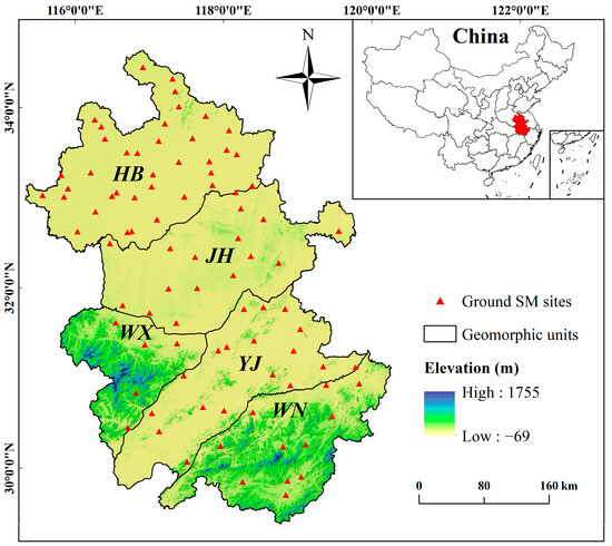
Figure 1.
Location of the study area.
HB is located in the north of Anhui province, accounting for about 27% of the total area, with flat terrain and fertile soil, making it the largest agricultural center in the province. JH covers around 23% of the total area, characterized by relatively low terrain and abundant water resources. YJ, spanning about 21% of the total area, is situated along the Yangtze River. It has a dense river network and well-developed paddy agriculture. WX and WN make up approximately 29% of the total area and are dominated by forest, with higher elevation.
2.2. Research Data
The data used in this study included ground measured SM, SMAP SM, MODIS products, Sentinel-1 data, DEM, soil property data, and precipitation data, all from the period of 1 April to 1 November 2019. Table 1 provides a description of these datasets.

Table 1.
Description of datasets used in this study.
2.2.1. Ground Measured SM Data
The ground measured SM data are provided by the Anhui Hydrology Bureau. There are 87 SM sites, of which 11 are located in WN, 5 in WX, 18 in YJ, 16 in JH, and 37 in HB (Figure 1). These sites collect SM data at three standard depths (10 cm, 20 cm, and 40 cm) on the 1st, 11th, and 21st of each month at 8:00 AM using the drying method. Validation of downscaling results with measured SM at 10 cm may introduce some uncertainty as the SMAP L4 represents SM at a depth of 5 cm. It has been demonstrated that SM of two consecutive soil layers is strongly correlated [28], therefore inconsistency in measurement depths has little effect on the correlation assessment. Theoretically, SM at 10 cm will be slightly higher than that at 5 cm as a result of infiltration and evapotranspiration.
2.2.2. SMAP SM Data
SMAP is a satellite mission launched by the National Aeronautics and Space Administration (NASA) in 2015 to monitor the global distribution of SM and freeze–thaw states at the Earth’s surface. The satellite is equipped with an L-band radar and an L-band radiometer, which synergistically enhance the accuracy and spatial resolution of SM retrievals [29]. The SMAP L4-SM data used in this study were acquired from the National Snow and Ice Data Centre (NSIDC) (https://nsidc.org/data/smap, accessed on 10 April 2023). It is generated every three hours, and data from 6:00 AM to 9:00 AM were selected to match the observation time of the measured SM.
2.2.3. Modis Products
MODIS is a crucial data source for constructing downscaling models in this study, providing continuous data with a spatial resolution of 250 m–1 km for important features such as spectral indices and surface temperature. All MODIS products used in this paper have been listed in Table 1, among which the MCD12Q1 provides LC data at 500 m resolution for 2019, MOD15A2H provides LAI data at 500 m every 8 days, and MOD11A1 provides LST data at 1 km per day. Additionally, MOD09A1 provides reflectance data at 500 m resolution every 8 days, and four spectral indices were calculated to provide information on surface vegetation, water bodies, and soils. The expressions for these indices are as follows:
where red, nir, blue, and green correspond to bands 1–4 of MODIS, and swir1 and swir2 correspond to bands 6–7, respectively. Furthermore, MCD43A3 provides albedo data in visible, near infrared, and shortwave bands. Since the difference between the mean values of white-sky albedo and black-sky albedo is small and highly correlated [30], their mean values in the shortwave band were used as an approximation of surface albedo in this study.
2.2.4. Sentinel-1 Data
Sentinel-1 is composed of two polar-orbiting satellites, Sentinel-1A and Sentinel-1B, both equipped with C-band synthetic aperture radar (SAR) sensors to monitor land and ocean surfaces. It has a 12-day repeat cycle and can operate in four imaging modes: strip map (SM), interferometric wide swath (IW), extra-wide swath (EW), and wave (WV). The IW mode is the main mode for land surface observation, providing 10 m resolution images in both VV and VH polarizations.
In this study, the ascending orbit data of Sentinel-1 in the IW mode were utilized, and a sliding time window processing method was applied to generate daily radar data. The window had a size of 12 days, containing 6 days before and after each day. This setup ensured that each day’s radar data had an equal temporal span, thus avoiding data gaps. Within the sliding time window, daily radar data were obtained by averaging all the Sentinel-1 images.
2.2.5. Topographic Data
Topography plays an important role in SM downscaling, which is closely related to the climate, surface runoff, and the water cycle, etc. The distribution of SM at different scales is strongly influenced by topography (e.g., elevation, slope), and many studies have used topographic features for SM downscaling [21]. In this study, the Shuttle Radar Topography Mission (SRTM) data from the GEE platform were used with a spatial resolution of 90 m.
2.2.6. Soil Property Data
Soil properties (proportion of clay, sand, and silt) are also vital predictors, which determine the permeability of surface water and the water-holding capacity of soil. The soil property data used in this study were downloaded from the Harmonized World Soil Database (HWSD) [31]. This dataset adopted the FAO-90 soil classification system, which encompassed physical and chemical characteristics of topsoil (0–30 cm) and subsoil (30–100 cm). The clay, sand, and silt data of topsoil were extracted and cropped to the study area.
2.2.7. Precipitation Data
Precipitation is another important climatic factor that affects SM dynamics besides surface temperature, and the soil response to rainfall differs across depths [32]. Time series precipitation data are commonly used to validate downscaled SM. The Climate Hazards Group InfraRed Precipitation with Station dataset (CHIRPS), which combines 0.05° resolution satellite imagery and in situ station data, is currently updated to version 2.0 and provides global precipitation data from 1981 to the present. In this study, CHIRPS data were acquired through the GEE platform as a validation set for the downscaling results.
2.2.8. Other SM Products
Two SM products with a spatial resolution of 1 km were selected for comparison with downscaled SM. The first is SMCI1.0 (Soil Moisture of China by in situ data, version 1.0), produced by Shangguan et al. [33]. It provides daily SM data from 2000 to 2020 and consists of 10 depth layers (10–100 cm), offering two versions with different resolutions of 30 s (~1 km) and 0.1 deg (~9 km). The product is available from the National Tibetan Plateau Science Data Center (https://cstr.cn/18406.11.Terre.tpdc.272415, accessed on 6 May 2023). This study obtained SMCI1.0 SM at 10 cm depth with a spatial resolution of 1 km as one of the validation datasets.
Moreover, SMAP released the SMAP-derived 1 km downscaled surface SM product (abbreviated as SMAP D-SM) in March 2023, which contains global daily 1 km resolution surface SM [34]. Currently version 1 data are available from the NSIDC Center, and daily SM data during the study period were obtained as another validation dataset (https://nsidc.org/data/smap, accessed on 25 April 2023). The product has two bands: band 1 represents the data for the ascending orbit (6 AM) and band 2 for the descending orbit (6 PM). Given the high number of missing values, we combined the two bands to fill in the missing values of the AM data with the PM data.
3. Methods
Section 3.1 illustrates the data preparation process based on GEE. Section 3.2 introduces three improved algorithms for GBDT: XGBoost, CatBoost, and LightGBM, which are tree-based ML methods that differ in model construction, feature processing, and target optimization. To integrate the advantages of the three models, this study adopts the Stacking strategy. This subsection can be realized with the scikit-learn library for Python3 and Jupyter Notebook. Section 3.3 demonstrates the overall downscaling strategy and provides a schematic diagram. Finally, Section 3.4 presents several metrics to evaluate the downscaling results.
3.1. Data Preparation
Some low-quality pixels may be observed in the MODIS products due to noise (mainly clouds). To maintain the spatial continuity and consistency of the data while minimizing the outliers, low-quality pixels were first filtered out through the quality control bands in each MODIS dataset. Then, for the daily-scale data (MOD11A1, MCD43A3), the missing values were filled in by linear interpolation using the valid values of the images within 15 days before and after. Similarly, for the 8-day scale data (MOD09A1, MOD15A2H), images of intermediate dates were generated by linear interpolation.
To further improve the quality and smoothness of the interpolated data, the SG (Savitzky–Golay) filter was introduced. This method utilizes polynomials for the least-squares fitting of values within a moving window, effectively removing noise while preserving the trend of data [35]. There are two important parameters of the SG filter, the half-width of the sliding window, m, and the order of the polynomial, d. Specifically, m determines the amount of data considered by the filter, while d defines the order of the polynomial used in the filter. A larger m and smaller d result in a smoother filtering result. After several tests, this study set m to 5 and d to 4.
MCD12Q1 is an annual product with five classification schemes. This study selected Land Cover Type 5, the Plant Functional Type (PFT) scheme, which includes 8 biomes and 4 other land cover types, totaling 12 types. The area of each class was calculated and reclassified to reduce the complexity and uncertainty of classification (Table 2). Water bodies were excluded to minimize the negative impacts on downscaling performance.
Table 2.
MCD12Q1 (PFT) land cover types and reclassification scheme.
3.2. Machine Learning Methods
3.2.1. XGBoost
XGBoost is an ensemble learning method based on the GBDT algorithm proposed by Chen and Guestrin [36]. Compared to the traditional GBDT algorithm, XGBoost adopts the second-order derivative to expedite model convergence, thereby enhancing optimization efficiency. It also incorporates a regularization term to control the model complexity. Moreover, XGBoost can handle samples with missing features by assigning them to the left or right subtrees based on their gain.
3.2.2. LightGBM
LightGBM was created by Microsoft in 2017 [37]. It is also based on GBDT and employs a histogram-splitting algorithm that greatly reduces the time complexity. Unlike other decision tree algorithms that operate level-wise, LightGBM uses a leaf-wise algorithm with depth limits, which reduces unnecessary computation. Additionally, LightGBM utilizes the gradient-based one-side sampling (GOSS) algorithm to remove samples with small gradients and prioritize under-trained data, making it particularly effective for handling large datasets.
3.2.3. CatBoost
CatBoost is based on oblivious trees, developed by Yandex [38]. Oblivious trees are a special type of decision tree that are characterized by the use of the same features for node division at each level, which can minimize the depth of the tree and memory consumption. By using the ordered boosting method, CatBoost addresses the prediction shift problem inherent in traditional gradient boosting algorithms, thus avoiding target leakage and overfitting.
3.2.4. Stacking Model
Current prevailing ensemble learning methods include Bagging, Boosting, and Stacking. Bagging and Boosting are homogeneous ensemble algorithms, and their base estimators are generated by the same algorithm. Stacking is a heterogeneous ensemble approach that observes different aspects of the data through different models. It is essentially a stratified structure where each layer can contain multiple estimators. In the case of two layers, the base estimator in the first layer receives its predictions from the training data and then passes them to the second layer for further study. This stratified structure allows different models to complement each other, ultimately creating a more powerful model. Considering the base models used in this study, the steps of Stacking are shown in Figure 2.
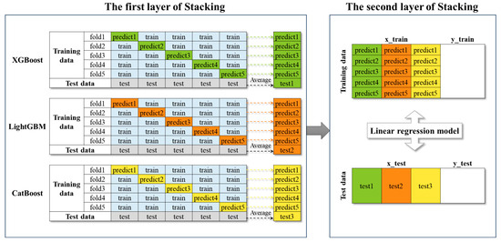
Figure 2.
Schematic of the Stacking strategy.
3.3. Construction of Downscaling Framework Based on Stacking Strategy
ML methods have been widely applied in SM downscaling. Some studies experiment directly with a single model, while others compare the performance of models during the training phase to select the best one. However, relying on a single model may not fully capture the complexity of SM distribution, especially when dealing with multiple influencing factors. This study proposed a Stacking fusion model for SM downscaling with a total of 15 predictors, including NDVI, NDWI, NSDSI, EVI, VV, VH, LAI, LST, Albedo, sand, silt, clay, DEM, LC, and DOY (day of that year). Figure 3 illustrates the framework of downscaling, specifically:
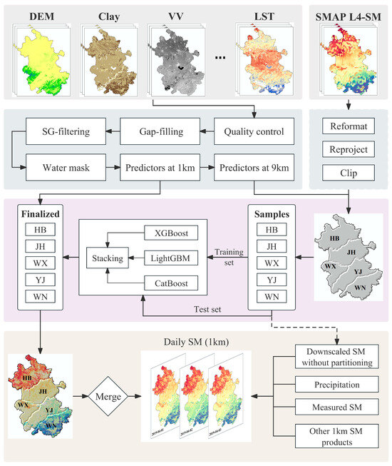
Figure 3.
Schematic of the proposed downscaling framework.
- Data preparation: in Section 3.1, we performed quality control, gap-filling, and SG filtering on MODIS data through the GEE platform, simplifying the land cover types and removing the water bodies.
- Data processing: To standardize the spatial resolution of all predictors to 1 km and 9 km, the MCD12Q1 dataset was aggregated using the mode method and the remaining datasets were aggregated using the mean method. The coordinate systems for all datasets were unified to the UTM projection system with WGS84 datum.
- Sample generation: The 9 km features and SMAP L4-SM were sampled according to the terrain partition (HB, JH, WX, YJ, WN). Besides remotely sensed features, DOY was added to indicate the generation time of features.
- Model construction: Taking the WN region as an example, the samples collected in this region were randomly divided into the training set and test set with a ratio of 7:3. XGBoost, LightGBM, and CatBoost were trained using the five-fold cross validation method and fused through the Stacking strategy. The test set was not involved in training and only used for model evaluation. It is worth mentioning that, to test the effectiveness of terrain partitioning, we also trained a Stacking model without partitioning.
- Model application: The trained Stacking models were then applied to the 1 km resolution features to generate downscaled SM for each region, and finally the downscaled results were merged by date.
- Validation: The downscaling results were validated using the measured SM from 87 sites, together with precipitation data. Furthermore, we compared the SMCI1.0 and SMAP D-SM products as well as the downscaled SM without partitioning.
3.4. Evaluation Method
To fully evaluate the proposed downscaling framework, several metrics were introduced [39]. The correlation coefficient (R) and the root mean square error (RMSE) were used to assess the performance of the trained model, measuring the difference between the predicted and true values. The bias and unbiased RMSE (ubRMSE) were also applied. UbRMSE is commonly used in SM downscaling studies, and the SMAP requirement for ubRMSE is less than 0.040 m3/m3. These four metrics are calculated as follows:
where E[•] represents the mean operator, and refer to the measured SM and SMAP SM; and and are the standard deviations of the SMAP SM and measured SM, respectively.
4. Results
4.1. Validation of Downscaling Framework
A total of 310,935 samples were obtained by sampling the feature dataset and SMAP L4 dataset at 9 km spatial resolution during the study period. For each region, XGBoost, LightGBM, and CatBoost models were trained using the five-fold cross validation method, and their prediction results were fused by the Stacking strategy. Table 3 displays the number of samples for each region and the performance of the models in the training and test sets. It is evident that all models achieved R values exceeding 0.9 and RMSE values below 0.028 m3/m3 on both training and testing sets, indicating a strong correlation between the model predictions and the actual values. The four models successfully captured the relationship among the features and target at a coarse scale. In addition, they exhibited similar R and RMSE values on their respective training and test sets, which further demonstrated that they were not overfitted.
Table 3.
Number of samples and performance of XGBoost, LightGBM, CatBoost and Stacking models on training and test sets for each region (HB, JH, WX, YJ, and WN). Bold indicates the best model score. The unit of RMSE is m3/m3.
The model’s performance on the test set determines its ability to generalize to unknown data. Figure 4 reveals that the Stacking model outperformed the others, with the highest R and the lowest RMSE in each region. XGBoost had comparable performance to Stacking model and was the most robust of the three base models. CatBoost also showed reliable accuracy, confirming its feasibility for the SM downscaling task. While LightGBM had the fastest training speed, its performance was slightly inferior to the other models. Surprisingly, the WN region had the best simulation results among the five regions (Stacking: R:0.989; RMSE:0.011 m3/m3), followed by the WX region (Stacking: R:0.981; RMSE:0.014 m3/m3), which may be attributed to the quality of the samples.
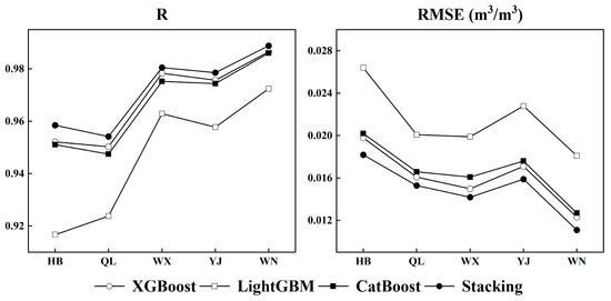
Figure 4.
Performance of XGBoost, LightGBM, CatBoost, and Stacking on the test set.
4.2. Overall Performance of Downscaled SM
Downscaled SM was validated using the measured SM data collected from April to November 2019. Figure 5 shows the distribution of R and ubRMSE values for 87 sites. Overall, most sites exhibited satisfactory performance. Regarding R values, 52 sites performed well (R > 0.60; 60% of the total), 26 sites showed moderate performance (0.4 < R < 0.6; 30%), and 9 sites performed poorly (R < 0.4; 10%), including one with extremely weak correlation (R < 0). The 9 poorly performing sites were mainly located in the HB and JH regions, characterized by flat terrain and predominantly agricultural, so the weaker correlation may be attributed to the irrigation conditions in these regions. This emphasizes the influence of human activities on SM and the sensitivity of the downscaling approach to such impacts. In addition, the average ubRMSE value for these 87 sites was 0.040 m3/m3, with 45 sites that met the SMAP accuracy requirements for ubRMSE (ubRMSE < 0.040 m3/m3), 38 sites showed acceptable errors (0.040 m3/m3 < ubRMSE < 0.060 m3/m3), and 4 sites underperformed (ubRMSE > 0.060 m3/m3), mainly in the JH and WN regions.
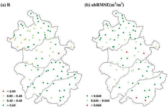
Figure 5.
Spatial distribution of (a) R and (b) ubRMSE between downscaled SM and measured SM at 87 SM sites from 1 April to 1 November 2019.
To further compare the downscaled SM across different regions, bias was introduced to assess the deviation between downscaled SM and measured SM. As shown in Figure 6, the positions of points represent the values of R and ubRMSE, and the colors reflect the bias values. Red indicates a dry bias, while blue signifies a wet bias, and the darker the color, the more severe the deviation. The results revealed that the downscaled SM in the HB and JH regions exhibited significant dry bias. Among the 37 sites in the HB region, 33 sites had bias values less than 0, as well as for 14 out of 16 sites in the JH region. The average bias values for these two regions were −0.050 m3/m3 and −0.034 m3/m3. Conversely, the WX, YJ, and WN regions displayed a clear wet bias, especially in the WN region, with average bias values of 0.029 m3/m3, 0.026 m3/m3, and 0.090 m3/m3, respectively. The fundamental reason for deviation was that the original SMAP products had certain uncertainties due to the coarse resolution as well as the effects of vegetation and surface roughness, which inevitably affected the performance of the downscaled SM. Moreover, the deviation was related to the methods of obtaining SM data at different scales. The measured SM was collected based on ground observations, representing specific SM values at 10 cm depth, while the downscaled SM represented approximate average SM values at 5 cm depth within 1 km.
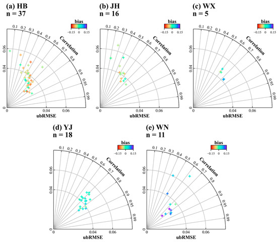
Figure 6.
The relationships between measured SM and downscaled SM. (a) HB, (b) JH, (c) WX, (d) YJ, and (e) WN. The color of the points represents the bias value. n represents the number of sites, and sites with a correlation coefficient less than 0 are excluded from the figure.
We compared all SM products with measured SM and plotted their R, bias, RMSE, and ubRMSE values. As shown in Figure 7, the downscaled SM generally had higher correlation coefficients, with a mean R value of 0.613 and a median R value of 0.659. SMAP L4-SM is the original coarse-resolution product, which had comparable accuracy with the downscaled SM (mean R: 0.605; median R: 0.648). Yet, the downscaled SM showed a significant reduction in R outliers. The downscaled SM(WP) is a downscaled version of SM obtained without partition modeling. It also showed reliable accuracy, with a mean R value of 0.551 and a median R value of 0.610. Compared with SMAP L4-SM, both downscaled SM and downscaled SM(WP) displayed a narrower range of bias values and were closer to 0. This may be explained by the fact that the downscaling process introduced more details, making the results closer to the measured SM. Although the RMSE values of the downscaled SM were slightly higher than downscaled SM(WP), its ubRMSE values were generally lower and exhibited less variability, suggesting higher overall accuracy. This demonstrated the feasibility of the Stacking model in SM downscaling field and proved the effectiveness of the terrain-based partitioning modeling strategy. The SMAP D-SM showed the most significant variation of all the metrics, implying the instability of its performance. This product consists of two bands representing SM values at 6 AM and 6 PM. Given the high number of missing values in a single band, the practice of using the 6 PM values to fill in the 6 AM missing values may have introduced additional uncertainties, leading to inconsistent overall performance. Furthermore, the algorithm of the product itself also has an impact. The SMCI1.0 product presented the lowest R level and the highest wet bias (mean bias: 0.089 m3/m3; median bias: 0.076 m3/m3), probably related to the data and method used by the authors. In summary, the Stacking model successfully improved the accuracy of SM, especially under the terrain partitioning modeling strategy.
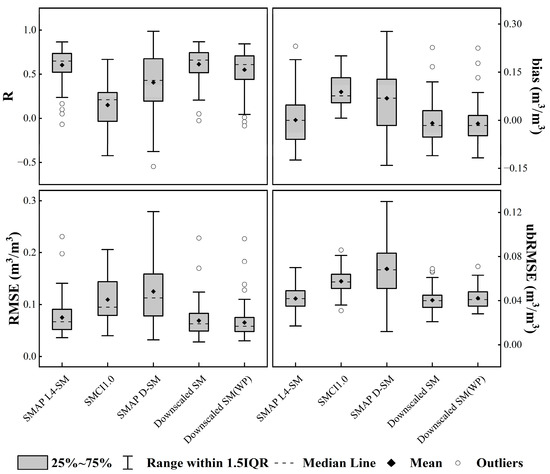
Figure 7.
Comparison of all SM products with measured SM. SMAP L4-SM denotes the original 9 km SMAP product. SMCI1.0 refers to the 1 km SM product of Shangguan et al. SMAP D-SM is the 1 km SM product released by SMAP in March 2023. Downscaled SM is the 1 km downscaling results of this study. Downscaled SM(WP) indicates the 1 km downscaling results without partition modeling.
4.3. Temporal Dynamics of Downscaled SM
To verify whether downscaled SM can capture the temporal dynamics of SM and respond to rainfall events, we randomly selected 11 sites and plotted a series of charts. In Figure 8, the first column shows the analysis results of all SM products (SMCI1.0, SMAP D-SM, SMAP L4-SM, downscaled SM, downscaled SM (WP)) along with measured SM, and precipitation data. The second column keeps only SMAP L4-SM, downscaled SM, and measured SM, highlighting the R, bias, and ubRMSE metrics before and after downscaling. We identified these sites using CODE-Region-LC numbers, where CODE stands for site code, Region for location, and LC for land cover type. The findings suggested that both downscaled SM and downscaled SM(WP) had strong temporally consistent behavior with SMAP L4-SM and captured the dynamic changes of SM. This observation was consistent for all sites. Surprisingly, downscaled SM eliminated the systematic deviation of SMAP to a certain extent, making the results closer to the measured SM. For instance, SMAP L4 underestimated the surface SM at site 50,637,471, resulting in a strong dry bias (bias = 0.094 m3/m3), while downscaled SM minimized it to 0.010 m3/m3. Similar dry bias corrections were found at sites 50,435,400 and 50,901,400. Overestimation can also be mitigated by downscaled SM, as exemplified by sites 62,905,301 and 70,140,600, where the bias was adjusted from 0.068 m3/m3 and 0.093 m3/m3 to 0.017 m3/m3 and −0.025 m3/m3, respectively.
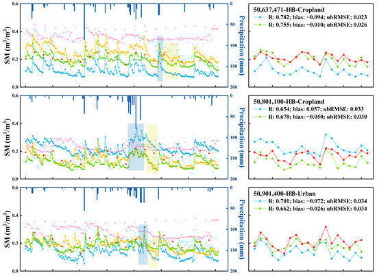
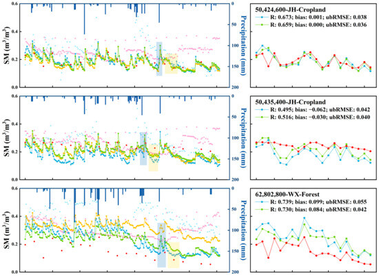
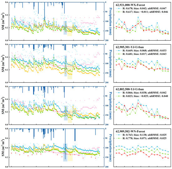
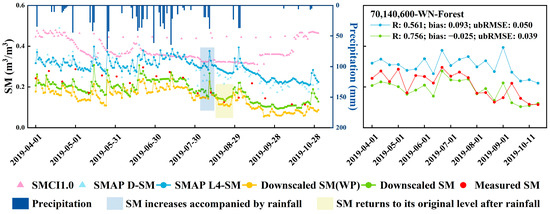
Figure 8.
Time series comparisons of SMCI1.0, SMAP D-SM, SMAP L4-SM, downscaled SM, downscaled SM (WP), measured SM, and precipitation data at 11 selected SM sites. Note: 2019-10-01 is not displayed because only one site had valid measured SM data on that day.
Although in some cases, the downscaled SM still had a large bias, such as the wet bias of 0.071 m3/m3 at site 62,909,502; there was already a noticeable improvement compared to the original SMAP L4-SM which had a wet bias of 0.138 m3/m3. In contrast, the bias correction ability of downscaled SM (WP) was relatively unstable. Some sites improved (50,801,100, 62,921,000), while others actually worsened (50,637,471, 62,802,800), which reaffirmed the advancement of the partitioning strategy. Moreover, Figure 8 illustrates that almost every rainfall event corresponded with an increase in SM, and both SMAP L4-SM and downscaled SM responded positively. The blue boxes in Figure 8 highlight significant increases in SM during rainfall events, and the yellow boxes indicate a gradual return of SM after rainfall. Such phenomena have existed at any time period. SMCI1.0 tended to overestimate at most sites, and SMAP D-SM fluctuated wildly, with only a few valid values from mid-June to August. This is consistent with the findings presented in Figure 7.
4.4. Spatial Distribution of Downscaled SM
To visualize the spatial heterogeneity of the downscaled SM, this section presents average distribution maps of SMAP L4-SM, downscaled SM, precipitation, LST during the study period, as well as DEM and clay. As can be seen from Figure 9, the downscaled SM not only retained the spatial pattern of the original SMAP L4-SM, but also provided a higher resolution. The SM pattern in Anhui Province presented a clear north–south variation, being lower in the north and higher in the south. Such difference is a consequence of combined climatic conditions, land cover, and topography [10]. The southern regions are located in the humid zone and enjoy abundant precipitation under the influence of monsoon. They are predominantly forested, which reduces water evaporation and runoff, thus increasing SM retention. Meanwhile, the northern areas experience a semi-humid climate characterized by limited precipitation. Coupled with extensive cultivation, the soil in this region is loose and has difficulty retaining water [40].
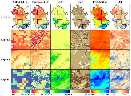
Figure 9.
Mean distribution maps from April to November 2019 for SMAP L4-SM, downscaled SM, precipitation, LST, and distribution maps for DEM and clay. Note that water bodies are not excluded from the plots.
We additionally conducted a detailed examination of three regions, labeled A, B, and C, which display unique topographic and climatic features. Region A is characterized by low elevation, limited precipitation, and high temperature; region C is marked by high elevation, abundant precipitation, and low temperature; and region B has a medium elevation between the two, with mild temperature and precipitation. The local maps show that downscaled SM was sensitive to changes in precipitation and LST, indicating its strong spatial heterogeneity. And the distribution of downscaled SM in the three regions demonstrated characteristics consistent with topography and climate: region A had generally low SM values, suggesting a drier environment; region C tended to have higher SM values, indicating ample water resources; and region B had intermediate SM values and did not show significant dryness or wetness. It is noteworthy that the downscaled SM showed high spatial correlation with DEM and clay, highlighting their dominant roles in the downscaling models, while other features modulate the local changes and heterogeneity of SM. This finding will be further verified in the subsequent section.
5. Discussion
5.1. Analysis of Input Predictors
We developed a SM downscaling framework based on the Stacking strategy using 15 predictors: NDVI, NDWI, NSDSI, EVI, VV, VH, LAI, LST, Albedo, sand, silt, clay, DEM, LC, and DOY, which successfully generated SM at 1 km resolution on a daily scale. The relative importance of the predictors and their effects on the model’s output were also investigated. The feature importance provided by the tree models can reveal some of the black-box nature of the model and identify the influential features, but they do not indicate the exact relationship between the features and target, such as positive or negative correlation. SHAP [41] values can measure the magnitude and direction of each feature’s influence. They treat each prediction as a collaborative result of all features and assign a SHAP value to each feature based on its contribution to the prediction. We used SHAP values to analyze how each feature affects the prediction result in this study. To approximate the SHAP values of the Stacking model, we combined the SHAP values of the XGBoost, LightGBM, and CatBoost models in each region on the training set. Feature importance was obtained by taking the mean of absolute SHAP values for each feature.
Figure 10 displays the SHAP values of the features for each region, with the most influential features near the top of the y-axis. It is evident that DOY plays the most crucial role in downscaling models for all regions. This suggests that it is advisable to introduce time as a feature since it can capture the seasonal variation of SM. Moreover, the time feature can help the model identify anomalous data caused by noise like cloud cover or signal interference and adjust the predicted values promptly. Shangguan et al. [42] also found the importance of the DOY in their study.
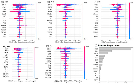
Figure 10.
SHAP values and feature importance of Stacking models in different regions: (a) HB, (b) JH, (c) WX, (d) YJ, and (e) WN. LC_1.0, LC_2.0, LC_3.0, and LC_4.0 are new features generated by the one-hot encoding of LC features. (f) Feature importance plot obtained by averaging the absolute values of SHAP values; note that the new features derived from one-hot encoding of LC have been summed up as LC.
Clay is the second most influential feature, which along with sand and silt, determines the physical properties of the soil, and in turn affects the storage and movement of SM [43]. Clay has the finest particles, and soils with more clay content generally have lower infiltration and permeability rates but higher water-holding capacity. Figure 10d shows a positive correlation between clay and SM, meaning that higher clay content leads to higher SM. Conversely, sand has the coarsest particles, and soils with more sand content have better permeability and drainage properties but lower water-holding capacity. Figure 10c demonstrates that sand is negatively correlated with SM, implying that higher sand content results in lower SM. Silt has a particle size between clay and sand, which can retain some water making the soil moist.
DEM is the third significant feature, supported by previous studies demonstrating that topography and soil property are crucial factors influencing SM dynamics [14,21]. In HB, JH, and YJ regions, DEM was negatively correlated with SM, which is consistent with the results of Fu et al. [44]. These regions have lower elevations, typically below 100 m, and mainly consist of cropland. The negative correlation may be due to the flat topography, which allows moisture to accumulate. Unlike other regions, WX and WN have higher elevations and are predominantly forested, where a positive trend in the correlation between DEM and SM is observed. This could be explained by the role of trees in improving soil water retention capacity [45]. Generally, higher elevations have more forest cover, while lower elevations are dominated by grasslands or croplands. Forested land has more canopy and leaves, which shade solar radiation and reduce heat from the soil surface, thereby increasing SM content. On the other hand, temperature variations caused by elevation change are also a significant factor; higher elevations usually have lower temperatures, which reduces the evaporation rate and favors SM retention. We plotted the co-interaction of DEM and LST on SM in the JH and WX regions (Figure 11). The results show that DEM was more variable in the WX region, and there was a noticeable interaction between LST and DEM. In areas with higher DEM, LST tended to be lower and SHAP values were positive, indicating a positive effect on SM. On the contrary, the JH region had a small range of DEM variation, and the interaction between LST and DEM was less pronounced. These findings suggest that the impact of DEM on SM is complex, and it depends not only on the variation of DEM itself but also on the interaction effects of DEM with other factors. This is exactly the purpose of our downscaling strategy based on terrain partitioning, which simplifies the complex influence of terrain and improves the stability and consistency of downscaling models.
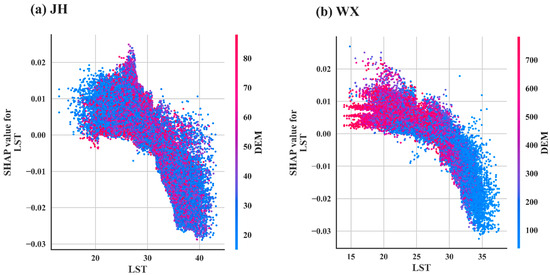
Figure 11.
Co-interaction of LST and DEM on SM in the JH and WX regions. (a) JH, (b) WX.
LST controls the surface thermal changes and is the most significant dynamic variable besides DOY. Many studies have confirmed its importance [13,46]. As shown in Figure 10, the red LST point is on the left side of the y-axis, which means the increase of LST will bring negative feedback to the SM. This finding is further supported by Figure 11, as the SHAP value is less than 0 when the LST exceeds about 25 °C, indicating a negative effect on SM at this point. Albedo is also of high importance as it represents the proportion of solar radiation reflected by the Earth’s surface. Studies have shown a typical exponential relationship between Albedo and SM, and the surface Albedo will decrease with the increase of SM [47]. This is due to the fact that wet soils are darker than dry soils and darker soils have lower albedo values. The negative correlation is more significant in the YJ, WX, and WN regions.
VV and VH have a certain penetration ability and can directly detect the surface SM. Figure 10f shows that VV is more significant than VH, which agrees with the findings of Bai [25]. It is noteworthy that the influence of vegetation on the backscattering coefficient under the VV mode is less than that of VH. This is because under VH polarization, the radar microwave is vertically transmitted and horizontally received, which is more susceptible to vegetation, resulting in more vegetation information in the backscatter. Whereas VV polarization is vertically transmitted and vertically received, and so this mode penetrates the vegetation better and contains more soil information in the backscatter.
Among the four spectral indices (NDVI, EVI, NDWI, and NSDSI), NSDSI has the highest importance, followed by NDWI and EVI, and NDVI is the least. NSDSI is an index calculated by the reflectance of the swir bands, which is sensitive to the changes of SM [48]. NDVI has been proven essential in previous SM downscaling studies, but it has little effect in this study. This is not an isolated case; Yang et al. [49] also found that NDVI had a low score in their study. The role of vegetation was significant in some studies [6,50], but others found that vegetation played a limited role at the 1 km scale [51]. This may be caused by the nonlinear and threshold effects of vegetation on SM, and the relationship between NDVI and SM may be positive, negative, or irrelevant for different vegetation cover. In terms of this study, these indices including LAI played a minor role in the downscaling models, while clay, DEM, and LST played a major role.
5.2. Uncertainty of This Study
Despite the encouraging results of our downscaling study, as with most studies, there are some unavoidable uncertainties. The first is the quality of the remote sensing data sources, including both the predictors and target. During the data preparation step, we performed interpolation and filtering operations on the quality-controlled feature datasets to obtain more reliable continuous data. In fact, there were still missing values and outliers, especially in the LST data. Missing values reduced the number of valid samples, while outliers interfered with the judgement of the downscaling models to make inaccurate predictions. On the other hand, the accuracy of downscaling results is highly dependent on the coarse-resolution SM products. Since the model was constructed based on the relationship between the aggregated high-resolution predictors and coarse-resolution SM products, the uncertainty of the original SM products directly affected the accuracy of the downscaling results. As can be seen from Figure 7 and Figure 8, SMAP L4 products tended to underestimate at lower SM levels (HB, JH) and overestimate at higher SM levels (WX, YJ, and WN). These uncertainties were propagated and amplified during the downscaling process, leading to biases in the downscaled SM. Future research should aim to enhance the reliability of data sources and minimize the losses associated with data quality.
The second uncertainty relates to scale. To align the resolution of the predictors with SMAP L4, the numerical features were aggregated using the average method. However, this process led to a loss of extreme values. For instance, the range of DEM changed from 1–1683 m to 4–1212 m. These extreme values reappeared when the model was applied, and the unlearned data may affect the accuracy of the model’s output.
The third uncertainty occurs in the validation phase since the measured SM and the remotely sensed SM have different depths and breadths. On the one hand, the measured SM is acquired manually by the drying method, which always represents the SM condition at a depth of 10 cm, while the remotely sensed SM is obtained by inverting the microwave signal. SMAP L4 claims that the depth of the surface SM is the top 5 cm of the soil, but the actual penetration depth of the microwave signal is not fixed and varies with the soil water content [52]. This means that the remotely sensed SM may contain SM information from different depths, not just from the top 5 cm. On the other hand, the measured SM only reflects the SM condition in a small area, while the downscaled SM represents the average SM condition within 1 km. In summary, the inconsistency of depth and breadth will affect the representativeness of the measured SM collected at a specific depth, thus reducing the comparability of the results.
6. Conclusions
This study proposed a downscaling framework for SMAP soil moisture based on a Stacking strategy that considers the geomorphic units. The spatial resolution of the SMAP L4-SM product was successfully improved from the original 9 km to 1 km by using multi-source datasets including: MODIS, Sentinel-1, topography, and soil property. The main findings are summarized as follows.
- The framework incorporated three ML models, XGBoost, LightGBM, and CatBoost. Comparison revealed that the Stacking model achieved the highest accuracy in all regions, followed by XGBoost, CatBoost, and LightGBM. Validation with measured SM showed that 60% of the sites were highly correlated with downscaled SM (R > 0.6), with an average ubRMSE of 0.040 m3/m3, which satisfied the accuracy requirements of the SMAP products. Moreover, the downscaling results outperformed the available 1 km resolution SM products (SMCI1.0, SMAP D-SM) and method without partitioning (downscaled SM (WP)).
- Both downscaled SM and downscaled SM (WP) exhibited temporal consistency with SMAP L4-SM and responded positively to rainfall events. They also mitigated the systematic bias of the SMAP L4 product, but downscaled SM (WP) performed inconsistently and sometimes even aggravated the bias. The spatial pattern analysis indicated that the downscaled SM preserved the overall trend of SMAP L4-SM while enriching the details. The downscaled SM was higher in the humid regions and lower in the semi-humid regions, which agreed with the actual situation.
- Among the 15 predictors, DOY, clay, and DEM were the most important and determined the overall distribution of SM. It is worth noting that the relationship between DEM and SM was complex; they exhibited a negative correlation in the plains and a positive correlation in the mountains. LST and Albedo reflected the dynamics of surface energy and showed a negative correlation with SM in all regions. VV polarization was less affected by vegetation and thus captured SM changes more effectively than VH. NSDSI was found to be more sensitive to SM than the other spectral indices, and together they regulated local variations and spatial heterogeneity of SM.
In conclusion, this study provides evidence supporting the applicability of the Stacking model in SM downscaling studies. Furthermore, it validates the effectiveness of the terrain-based partitioning strategy. Future studies can further explore the effects of long series data in practical applications, such as assessing the response of SM to climate change and human activities and analyzing the variability of downscaling results in different seasons.
Author Contributions
Conceptualization, J.X., J.M. and X.L.; methodology, J.X. and L.Z.; software, J.M. and W.S.; validation, J.X., X.L. and J.M.; formal analysis, J.X., Q.S. and X.S.; investigation, J.X., X.S. and X.L.; resources, X.L., W.S. and J.M.; data curation, J.X. and L.Z.; writing—original draft preparation, J.X.; writing—review and editing, J.X., X.L. and J.M.; visualization, J.X. and L.Z.; supervision, X.L., J.M. and Q.S.; project administration, J.X. and W.S.; funding acquisition, X.L. and W.S. All authors have read and agreed to the published version of the manuscript.
Funding
This research was funded by the Three Gorges Follow-up Work “Remote Sensing Investigation and Evaluation of Flood Control Safety in the Three Gorges Section” (JZ0161A012023); the Youth Innovation Talents Promotion Plan of the Research Center of Flood and Drought Disaster Reduction of the Ministry of Water Resources; and the Key Research and Development Program of Jiang Xi Province (20212BBG71008).
Data Availability Statement
The data presented in this study are available upon request from the corresponding author.
Acknowledgments
The authors would like to thank the National Snow and Ice Data Center for providing the SMAP product, the Harmonized World Soil Database for providing the soil property data, and the Google Earth Engine platform for providing the remotely sensed data, which are available to all users free of charge. We also thank the Anhui Hydrology Bureau for providing the measured soil moisture data. Finally, we sincerely appreciate the suggestions and comments made by the reviewers and the managing editor, which improved this paper.
Conflicts of Interest
The authors declare no conflicts of interest.
References
- Huntington, T.G. Evidence for intensification of the global water cycle: Review and synthesis. J. Hydrol. 2006, 319, 83–95. [Google Scholar] [CrossRef]
- Seneviratne, S.I.; Corti, T.; Davin, E.L.; Hirschi, M.; Jaeger, E.B.; Lehner, I.; Orlowsky, B.; Teuling, A.J. Investigating soil moisture-climate interactions in a changing climate: A review. Earth Sci. Rev. 2010, 99, 125–161. [Google Scholar] [CrossRef]
- Dorigo, W.A.; Wagner, W.; Hohensinn, R.; Hahn, S.; Paulik, C.; Xaver, A.; Gruber, A.; Drusch, M.; Mecklenburg, S.; van Oevelen, P.; et al. The International Soil Moisture Network: A data hosting facility for global in situ soil moisture measurements. Hydrol. Earth Syst. Sci. 2011, 15, 1675–1698. [Google Scholar] [CrossRef]
- Qin, J.; Yang, K.; Lu, N.; Chen, Y.Y.; Zhao, L.; Han, M.L. Spatial upscaling of in-situ soil moisture measurements based on MODIS-derived apparent thermal inertia. Remote Sens. Environ. 2013, 138, 1–9. [Google Scholar] [CrossRef]
- Paloscia, S.; Pettinato, S.; Santi, E.; Notarnicola, C.; Pasolli, L.; Reppucci, A. Soil moisture mapping using Sentinel-1 images: Algorithm and preliminary validation. Remote Sens. Environ. 2013, 134, 234–248. [Google Scholar] [CrossRef]
- Abbaszadeh, P.; Moradkhani, H.; Zhan, X.W. Downscaling SMAP Radiometer Soil Moisture Over the CONUS Using an Ensemble Learning Method. Water Resour. Res. 2019, 55, 324–344. [Google Scholar] [CrossRef]
- Liu, J.; Chai, L.N.; Lu, Z.; Liu, S.M.; Qu, Y.Q.; Geng, D.Y.; Song, Y.Z.; Guan, Y.B.; Guo, Z.X.; Wang, J.; et al. Evaluation of SMAP, SMOS-IC, FY3B, JAXA, and LPRM Soil Moisture Products over the Qinghai-Tibet Plateau and Its Surrounding Areas. Remote Sens. 2019, 11, 792. [Google Scholar] [CrossRef]
- Entekhabi, D.; Njoku, E.G.; O’Neill, P.E.; Kellogg, K.H.; Crow, W.T.; Edelstein, W.N.; Entin, J.K.; Goodman, S.D.; Jackson, T.J.; Johnson, J.; et al. The Soil Moisture Active Passive (SMAP) Mission. Proc. IEEE 2010, 98, 704–716. [Google Scholar] [CrossRef]
- Zhao, W.; Wen, F.; Cai, J. Methods, progresses and challenges of passive microwave soil moisture spatial downscaling. Natl. Remote Sens. Bull. 2022, 26, 1699–1722. [Google Scholar] [CrossRef]
- Peng, J.; Loew, A.; Merlin, O.; Verhoest, N.E.C. A review of spatial downscaling of satellite remotely sensed soil moisture. Rev. Geophys. 2017, 55, 341–366. [Google Scholar] [CrossRef]
- Sabaghy, S.; Walker, J.P.; Renzullo, L.J.; Jackson, T.J. Spatially enhanced passive microwave derived soil moisture: Capabilities and opportunities. Remote Sens. Environ. 2018, 209, 551–580. [Google Scholar] [CrossRef]
- Srivastava, P.K.; Han, D.W.; Ramirez, M.R.; Islam, T. Machine Learning Techniques for Downscaling SMOS Satellite Soil Moisture Using MODIS Land Surface Temperature for Hydrological Application. Water Resour. Manag. 2013, 27, 3127–3144. [Google Scholar] [CrossRef]
- Wei, Z.S.; Meng, Y.Z.; Zhang, W.; Peng, J.; Meng, L.K. Downscaling SMAP soil moisture estimation with gradient boosting decision tree regression over the Tibetan Plateau. Remote Sens. Environ. 2019, 225, 30–44. [Google Scholar] [CrossRef]
- Karthikeyan, L.; Mishra, A.K. Multi-layer high-resolution soil moisture estimation using machine learning over the United States. Remote Sens. Environ. 2021, 266, 19. [Google Scholar] [CrossRef]
- Rao, P.Z.; Wang, Y.C.; Wang, F.; Liu, Y.; Wang, X.Y.; Wang, Z. Daily soil moisture mapping at 1 km resolution based on SMAP data for desertification areas in northern China. Earth Syst. Sci. Data 2022, 14, 3053–3073. [Google Scholar] [CrossRef]
- Yan, R.; Bai, J.J. A New Approach for Soil Moisture Downscaling in the Presence of Seasonal Difference. Remote Sens. 2020, 12, 2818. [Google Scholar] [CrossRef]
- Gao, B.H.; He, Y.; Chen, X.Y.; Zheng, X.Y.; Zhang, L.F.; Zhang, Q.; Lu, J.G. Landslide Risk Evaluation in Shenzhen Based on Stacking Ensemble Learning and InSAR. IEEE J. Sel. Top. Appl. Earth Obs. Remote Sens. 2023, 16, 1–18. [Google Scholar] [CrossRef]
- Zhang, Y.Z.; Ma, J.; Liang, S.L.; Li, X.S.; Liu, J.D. A stacking ensemble algorithm for improving the biases of forest aboveground biomass estimations from multiple remotely sensed datasets. GISci. Remote Sens. 2022, 59, 234–249. [Google Scholar] [CrossRef]
- Zhen, M.; Yi, M.; Luo, T.; Wang, F.; Yang, K.; Ma, X.; Cui, S.; Li, X. Application of a Fusion Model Based on Machine Learning in Visibility Prediction. Remote Sens. 2023, 15, 1450. [Google Scholar] [CrossRef]
- Bentejac, C.; Csorgo, A.; Martinez-Munoz, G. A comparative analysis of gradient boosting algorithms. Artif. Intell. Rev. 2021, 54, 1937–1967. [Google Scholar] [CrossRef]
- Huang, S.Z.; Zhang, X.; Wang, C.; Chen, N.C. Two-step fusion method for generating 1 km seamless multi-layer soil moisture with high accuracy in the Qinghai-Tibet plateau. ISPRS J. Photogramm. Remote Sens. 2023, 197, 346–363. [Google Scholar] [CrossRef]
- Huang, G.M.; Wu, L.F.; Ma, X.; Zhang, W.Q.; Fan, J.L.; Yu, X.; Zeng, W.Z.; Zhou, H.M. Evaluation of CatBoost method for prediction of reference evapotranspiration in humid regions. J. Hydrol. 2019, 574, 1029–1041. [Google Scholar] [CrossRef]
- Li, H.M.; Zhang, G.L.; Zhong, Q.C.; Xing, L.Q.; Du, H.Q. Prediction of Urban Forest Aboveground Carbon Using Machine Learning Based on Landsat 8 and Sentinel-2: A Case Study of Shanghai, China. Remote Sens. 2023, 15, 284. [Google Scholar] [CrossRef]
- Carlson, T. An overview of the “triangle method” for estimating surface evapotranspiration and soil moisture from satellite imagery. Sensors 2007, 7, 1612–1629. [Google Scholar] [CrossRef]
- Bai, J.Y.; Cui, Q.; Zhang, W.; Meng, L.K. An Approach for Downscaling SMAP Soil Moisture by Combining Sentinel-1 SAR and MODIS Data. Remote Sens. 2019, 11, 2736. [Google Scholar] [CrossRef]
- Zhang, Y.F.; Liang, S.L.; Zhu, Z.L.; Ma, H.; He, T. Soil moisture content retrieval from Landsat 8 data using ensemble learning. ISPRS J. Photogramm. Remote Sens. 2022, 185, 32–47. [Google Scholar]
- Wang, C.H.; Lin, Q.G.; Wang, L.B.; Jiang, T.; Su, B.D.; Wang, Y.J.; Mondal, S.K.; Huang, J.L.; Wang, Y. The influences of the spatial extent selection for non-landslide samples on statistical-based landslide susceptibility modelling: A case study of Anhui Province in China. Nat. Hazard. 2022, 112, 1967–1988. [Google Scholar] [CrossRef]
- Kedzior, M.; Zawadzki, J. Comparative study of soil moisture estimations from SMOS satellite mission, GLDAS database, and cosmic-ray neutrons measurements at COSMOS station in Eastern Poland. Geoderma. 2016, 283, 21–31. [Google Scholar] [CrossRef]
- Reichle, R.; De Lannoy, G.; Koster, R.D.; Crow, W.T.; Kimball, J.S.; Liu, Q.; Bechtold, M. SMAP L4 Global 3-hourly 9 km EASE-Grid Surface and Root Zone Soil Moisture Geophysical Data, 7th ed.; Distributed by NASA National Snow and Ice Data Center Distributed Active Archive Center, 2022. [Google Scholar] [CrossRef]
- Wang, Z.S.; Schaaf, C.B.; Sun, Q.S.; Shuai, Y.M.; Roman, M.O. Capturing rapid land surface dynamics with Collection V006 MODIS BRDF/NBAR/Albedo (MCD43) products. Remote Sens. Environ. 2018, 207, 50–64. [Google Scholar] [CrossRef]
- Fischer, G.; Nachtergaele, F.; Prieler, S.; van Velthuizen, H.T.; Verelst, L.; Wiberg, D. Global Agro-ecological Zones Assessment for Agriculture (GAEZ 2008); IIASA: Laxenburg, Austria; FAO: Rome, Italy, 2008. [Google Scholar]
- Chen, L.; Zhang, K.L.; Zhang, Z.D.; Cao, Z.H.; Ke, Q.H. Response of soil water movement to rainfall under different land uses in karst regions. Environ. Earth Sci. 2023, 82, 17. [Google Scholar] [CrossRef]
- Shangguan, W.; Li, Q.; Shi, G. A 1 km Daily Soil Moisture Dataset over China Based on Situ Measurement (2000–2020); National Tibetan Plateau Data Center, 2022. [Google Scholar]
- Lakshmi, V.; Fang, B. SMAP-Derived 1-km Downscaled Surface Soil Moisture Product, Version 1; Distributed by NASA National Snow and Ice Data Center Distributed Active Archive Center, 2023. [Google Scholar] [CrossRef]
- Chen, J.; Jonsson, P.; Tamura, M.; Gu, Z.; Matsushita, B.; Eklundh, L. A simple method for reconstructing a high-quality NDVI time-series data set based on the Savitzky-Golay filter. Remote Sens. Environ. 2004, 91, 332–344. [Google Scholar] [CrossRef]
- Chen, T.; Guestrin, C. Xgboost: A scalable tree boosting system. In Proceedings of the 22nd ACM SIGKDD International Conference on Knowledge Discovery and Data Mining, San Francisco, CA, USA, 13–17 August 2016; pp. 785–794. [Google Scholar]
- Ke, G.; Meng, Q.; Finley, T.; Wang, T.; Chen, W.; Ma, W.; Ye, Q.; Liu, T.Y. Lightgbm: A highly efficient gradient boosting decision tree. In Proceedings of the 31st Conference on Neural Information Processing Systems (NIPS 2017), Long Beach, CA, USA, 8–9 December 2017; p. 30. [Google Scholar]
- Prokhorenkova, L.; Gusev, G.; Vorobev, A.; Dorogush, A.V.; Gulin, A. CatBoost: Unbiased boosting with categorical features. Adv. Neural Inf. Process. Syst. 2018, 6637–6647. [Google Scholar]
- Xu, M.Y.; Yao, N.; Yang, H.X.; Xu, J.; Hu, A.N.; de Goncalves, L.G.G.; Liu, G. Downscaling SMAP soil moisture using a wide & deep learning method over the Continental United States. J. Hydrol. 2022, 609, 22. [Google Scholar]
- Liu, X.W.; Zhang, X.Y.; Chen, S.Y.; Sun, H.Y.; Shao, L.W. Subsoil compaction and irrigation regimes affect the root-shoot relation and grain yield of winter wheat. Agric. Water Manag. 2015, 154, 59–67. [Google Scholar] [CrossRef]
- Lundberg, S.M.; Lee, S.I. A Unified Approach to Interpreting Model Predictions. Adv. Neural Inf. Process. Syst. 2017, 30, 1–10. [Google Scholar]
- Shangguan, Y.L.; Min, X.X.; Shi, Z. Inter-comparison and integration of different soil moisture downscaling methods over the Qinghai-Tibet Plateau. J. Hydrol. 2023, 617, 17. [Google Scholar] [CrossRef]
- Xu, X.L.; Ma, K.M.; Fu, B.J.; Song, C.J.; Liu, W. Relationships between vegetation and soil and topography in a dry warm river valley, SW China. Catena 2008, 75, 138–145. [Google Scholar] [CrossRef]
- Fu, H.; Yuan, G.X.; Ge, D.B.; Li, W.; Zou, D.S.; Huang, Z.R.; Wu, A.P.; Liu, Q.L.; Jeppesen, E. Cascading effects of elevation, soil moisture and soil nutrients on plant traits and ecosystem multi-functioning in Poyang Lake wetland, China. Aquat. Sci. 2020, 82, 10. [Google Scholar] [CrossRef]
- Chia, R.W.; Yong, L.J.; Jang, J.; Lee, S.-b. Effects of land use change on soil moisture content at different soil depths. J. Geol. Soc. Korea 2022, 58, 117–135. [Google Scholar] [CrossRef]
- Zhao, W.; Sanchez, N.; Lu, H.; Li, A.N. A spatial downscaling approach for the SMAP passive surface soil moisture product using random forest regression. J. Hydrol. 2018, 563, 1009–1024. [Google Scholar] [CrossRef]
- Guan, X.D.; Huang, J.P.; Guo, N.; Bi, J.R.; Wang, G.Y. Variability of Soil Moisture and Its Relationship with Surface Albedo and Soil Thermal Parameters over the Loess Plateau. Adv. Atmos. Sci. 2009, 26, 692–700. [Google Scholar] [CrossRef]
- Sadeghi, M.; Jones, S.B.; Philpot, W.D. A linear physically-based model for remote sensing of soil moisture using short wave infrared bands. Remote Sens. Environ. 2015, 164, 66–76. [Google Scholar] [CrossRef]
- Yang, Z.J.; He, Q.S.; Miao, S.Q.; Wei, F.; Yu, M.X. Surface Soil Moisture Retrieval of China Using Multi-Source Data and Ensemble Learning. Remote Sens. 2023, 15, 2786. [Google Scholar] [CrossRef]
- Hu, F.M.; Wei, Z.S.; Zhang, W.; Dorjee, D.; Meng, L.K. A spatial downscaling method for SMAP soil moisture through visible and shortwave-infrared remote sensing data. J. Hydrol. 2020, 590, 11. [Google Scholar] [CrossRef]
- Joshi, C.; Mohanty, B.P. Physical controls of near-surface soil moisture across varying spatial scales in an agricultural landscape during SMEX02. Water Resour. Res. 2010, 46, 21. [Google Scholar] [CrossRef]
- Piles, M.; Camps, A.; Vall-Llossera, M.; Corbella, I.; Panciera, R.; Rudiger, C.; Kerr, Y.H.; Walker, J. Downscaling SMOS-Derived Soil Moisture Using MODIS Visible/Infrared Data. IEEE Trans. Geosci. Remote Sens. 2011, 49, 3156–3166. [Google Scholar] [CrossRef]
Disclaimer/Publisher’s Note: The statements, opinions and data contained in all publications are solely those of the individual author(s) and contributor(s) and not of MDPI and/or the editor(s). MDPI and/or the editor(s) disclaim responsibility for any injury to people or property resulting from any ideas, methods, instructions or products referred to in the content. |
© 2024 by the authors. Licensee MDPI, Basel, Switzerland. This article is an open access article distributed under the terms and conditions of the Creative Commons Attribution (CC BY) license (https://creativecommons.org/licenses/by/4.0/).